Refocusing of Ground Moving Targets with Doppler Ambiguity Using Keystone Transform and Modified Second-Order Keystone Transform for Synthetic Aperture Radar

Abstract

Ground moving targets will typically be defocused because of the range migration (RM) and Doppler frequency migration (DFM) caused by the unknown relative motions between the platform of synthetic aperture radar (SAR) and the ground moving targets. The received signal of the ground moving target easily exhibits the Doppler ambiguity, and the Doppler ambiguity leads to the refocusing difficulty of ground moving targets. To address these problems, a SAR refocusing method of ground moving targets with Doppler ambiguity based on modified second-order keystone transform (MSOKT) and keystone transform (KT) is presented in this paper. Firstly, the second-order phase is separated by the time reversing process. Secondly, MSOKT is performed to compensate the range curvature migration and DFM, and then the coefficient of the second-order phase is estimated. Finally, a well-refocused result of the moving target is achieved after KT and the estimated Doppler ambiguity number are used to eliminate residual range walk migration. The proposed method can accurately remove RM and DFM and effectively focus the moving targets without residual correction errors. Moreover, the effects of Doppler ambiguity (including Doppler center blur and spectrum split) and blind speed sidelobe are further avoided. On the basis of the analysis of cross-term for the multiple target case, the identification strategy of spurious peak of cross-term is proposed. Additionally, the developed method can be sped up by nonuniform fast Fourier transform without the interpolation operation. The effectiveness of the proposed method is verified by both airborne and spaceborne real data processing results.

1. Introduction

Synthetic aperture radar (SAR) can image the observed scenes under all-time and all-weather conditions, and it is receiving more and more attention all around the world [1,2,3,4,5,6]. It has been widely applied in modern remote sensing fields, for example, sea surface surveillance, ground traffic monitoring, and anti-terrorism. A number of moving targets inevitably appear in the observation scene. Therefore, the refocusing of ground moving targets has become an important function for SAR systems due to the huge demand for the monitoring of moving targets [7,8,9,10,11,12,13,14].

Nevertheless, the unknown relative motions between the SAR platform and ground moving targets result in severe defocusing effects, such as the effects of range migration (RM) in the range dimension and Doppler frequency migration (DFM) in the azimuth Doppler frequency dimension [12,13,15,16]. RM usually consists of two parts: the first part is range walk migration (RWM) caused by the cross-track velocity of ground moving targets; the second part is range curvature migration (RCM) induced by the along-track velocity of ground moving targets. Additionally, DFM is generally induced by the along-track velocity of ground moving targets. Given the limitation of pulse repetition frequency (PRF) for SAR systems, the received signal of ground moving targets easily exhibits the Doppler ambiguity [15,16]. The Doppler ambiguity includes Doppler center blur and spectrum split [12,13]. Both Doppler center blur and spectrum split induce difficulty in refocusing the ground moving targets. Therefore, RM, DFM and Doppler ambiguity are key problems for ground moving target refocusing, and they should be effectively addressed.

Recently, several approaches have been developed to address RM. The Hough/Radon transforms [17,18] were utilized to search the trajectory of moving targets to correct RWM. However, they suffer from the problem of high computational complexity. The keystone transform [19,20,21] has been proposed to remove RWM without searching the trajectory of ground moving targets. Although this method can correct RWM without knowing priori motion information of ground moving targets, it suffers from the effect of RCM. To address the problem of RCM, the second-order keystone transform (SOKT) [22,23] has been presented. Then, the Doppler KT (DKT) [24] has been introduced to deal with the effects of RWM and RCM, simultaneously. However, these transforms (i.e., KT, SOKT and DKT) cannot deal with the problems of DFM and Doppler ambiguity. To address these issues, the multi-dimensional searching methods [25,26,27] have been presented. Although these methods can effectively focus the moving targets, they still suffer from the huge computational burden given that their processing procedures have multi-dimensional searching steps. In order to reduce the computational complexity, the deramp-keystone and stationary phase-based methods [15,16] have been proposed to refocus the ground moving targets. However, these approaches apply the priori velocity of the SAR platform and ignore the along-track velocity of ground moving targets to approximately remove RCM and DFM, leading to serious defocusing effects. The improved axis rotation–time reversal transform (IAR–TRT) approach [13] has been developed to refocus the moving targets without ignoring the effect of the moving target’s along-track velocity. However, the performance of the IAR–TRT approach suffers from the effect of scaled frequency spectrum aliasing. Subsequently, the cross-track velocity-matching method [12] has been proposed in consideration of the scaled frequency spectrum aliasing. However, the performance of the cross-track velocity-matching method is deteriorated by the serious blind speed sidelobe (BSSL).

Motivated by previous work, in order to accurately compensate RM and DFM and refocus moving targets in the presence of Doppler ambiguity with a low computational burden, a SAR refocusing method for ground moving targets with Doppler ambiguity is presented. Notably, this paper is an extension of our previous work [28]. It considers the refocusing of the ground moving targets for SAR. Firstly, the time revering process step is applied to separate the second-order phase. Secondly, RCM and DFM are simultaneously eliminated by modified SOKT (MSOKT) and the estimated result of second-order phase coefficient is obtained. Then, KT is adopted to remove RWM induced by the baseband cross-track velocity of ground moving targets. Lastly, the residual RWM is removed by the estimated Doppler ambiguity number and the result of ground moving target refocusing is achieved. In addition, the interference of cross-term for multiple target refocusing is analyzed, and then the spurious peak recognition strategy is proposed to eliminate the effect of the cross-term. Both airborne and spaceborne real data processing results are presented to confirm the effectiveness of the proposed method.

The rest of this paper is organized as follows. Section 2 provides the signal model. Section 3 shows a description of the proposed algorithm. Section 4 gives the simulation experimental results. Section 5 presents the airborne and spaceborne real data processing results. The discussion is provided in Section 6. The conclusions are given in Section 7.

2. Signal Model

The side-looking strip-map mode SAR is considered. Figure 1 displays the motion geometry between the SAR platform with constant velocity $v$ and ground moving target on the 2D slant rang plane. During the integration time $T_i$, the moving target travels from point A to B, where $v_c$ and $v_a$ indicate the cross-track velocity and along-track velocity, respectively. As illustrated in Figure 1, the nearest and instantaneous slant range between the radar platform and moving target are denoted by $R_0$ and $R_s\left(t_n\right)$, respectively. The azimuth-time (slow-time) variable is represented by $t_n$.

Assume that the widely-used linear frequency modulation (LFM) signal is used as the transmitted signal with the form as follows [19]:

$$s\left(t\right)=\mathrm{r}\mathrm{e}\mathrm{c}\mathrm{t}(\frac{t}{T_p})\exp (j2\pi f_{c}t+j\pi \gamma t^2)$$

(1)

where $t$ denotes the range-time (fast-time) variable, $\mathrm{r}\mathrm{e}\mathrm{c}\mathrm{t}(\cdot )$ indicates the range window function, $T_p$ is the pulse duration of the transmitted signal, $\gamma$ denotes the chirp rate of the transmitted LFM signal, and $f_c$ represents the carrier frequency of transmitted signal. After down-converting is applied, the baseband signal of the raw echo omitting the amplitude can be expressed as follows [29]:

$$\begin{array}{c}{s}_b\left(t,t_n\right)=\mathrm{r}\mathrm{e}\mathrm{c}\mathrm{t}\left[\frac{t-2R_s\left(t_n\right)/c}{T_p}\right]w\left(t_n\right)\mathrm{e}\mathrm{x}\mathrm{p}\left\{j\pi \gamma {\left[t-\frac{2R_s\left(t_n\right)}{c}\right]}^2\right\}\\ \times \mathrm{e}\mathrm{x}\mathrm{p}\left[-j\frac{4\pi f_c}{c}{R}_s\left(t_n\right)\right]\end{array}$$

(2)

where $c$ denotes the speed of light and $w\left(\cdot \right)$ is the slow-time window function.

After the range compression is performed to Equation (2), the corresponding result in the range- and azimuth-time domain can be denoted as [16,19,29]:

$$s_1\left(t,t_n\right)=\mathrm{s}\mathrm{i}\mathrm{n}\mathrm{c}\left\{B\left[t-\frac{2R_s\left(t_n\right)}{c}\right]\right\}w\left(t_n\right)\mathrm{e}\mathrm{x}\mathrm{p}\left[-\frac{j4\pi f_c}{c}{R}_s\left(t_n\right)\right]$$

(3)

where $\mathrm{s}\mathrm{i}\mathrm{n}\mathrm{c}\left(x\right)=\mathrm{s}\mathrm{i}\mathrm{n}\left(\pi x\right)/\left(\pi x\right)$ indicates the sinc function and $B=\gamma T_p$ represents the range bandwidth.

In accordance with Figure 1, $R_s\left(t_n\right)$ can be written as follows:

$$R_s\left(t_n\right)=\sqrt{{\left(v{t}_n-v_a{t}_n\right)}^2+{\left(R_0-v_c{t}_n\right)}^2}$$

(4)

On the basis of Taylor series expansion, the instantaneous slant range $R_s\left(t_n\right)$ can be expanded as a second-order range model as follows [12,13,15,16]:

$$R_s\left(t_n\right)\approx R_0+{\rho }_1{t}_n+{\rho }_2{t}_n^2$$

(5)

where ${\rho }_1=-v_c$ and ${\rho }_2={\left(v-v_a\right)}^2/2R_0$ denote the first- and second-order phase coefficients, respectively.

Substituting Equation (5) into Equation (3), we have:

$$\begin{array}{c}{s}_2\left(t,t_n\right)=\mathrm{s}\mathrm{i}\mathrm{n}\mathrm{c}\left\{B\left[t-2\left(R_0-v_c{t}_n+\frac{{\left(v-v_a\right)}^2}{2R_0}{t}_n^2\right)/c\right]\right\}\\ \times w\left(t_n\right)\mathrm{e}\mathrm{x}\mathrm{p}\left[-\frac{j4\pi f_c}{c}\left(R_0-v_c{t}_n+\frac{{\left(v-v_a\right)}^2}{2R_0}{t}_n^2\right)\right]\end{array}$$

(6)

After the range fast Fourier transform (FFT) is applied to Equation (6), the corresponding received signal in the range-frequency and azimuth-time domain can be expressed as:

$$s_1\left(f,t_n\right)=\mathrm{r}\mathrm{e}\mathrm{c}\mathrm{t}\left(\frac{f}{B}\right)w\left(t_n\right)\mathrm{e}\mathrm{x}\mathrm{p}\left[-\frac{j4\pi }{c}\left(f+f_c\right)\right.\left.\left(R_0-v_c{t}_n+\frac{{\left(v-v_a\right)}^2}{2R_0}{t}_n^2\right)\right]$$

(7)

where the range-frequency variable is denoted by $f$.

As described in the exponential term of Equation (6), the $t_n$-term will induce Doppler center shift (DCS) in the azimuth Doppler frequency dimension. If DCS is larger than PRF/2, the received echo signal of the ground moving target will show Doppler center blur. Under this case, the cross-track velocity $v_c$ of the moving target can be rewritten as follows:

$$v_c=v_0+k_{\mathrm{a}}\frac{c\mathrm{P}\mathrm{R}\mathrm{F}}{2f_c}$$

(8)

where $v_0\in \left[-c\mathrm{P}\mathrm{R}\mathrm{F}/\left(4f_c\right){,}_{}c\mathrm{P}\mathrm{R}\mathrm{F}/\left(4f_c\right)\right]$ indicates the baseband cross-track velocity and the Doppler ambiguity number is denoted by $k_a$.

Substituting Equation (8) into Equation (7) yields:

$$\begin{array}{c}{s}_2\left(f,t_n\right)=\mathrm{r}\mathrm{e}\mathrm{c}\mathrm{t}\left(\frac{f}{B}\right)\mathrm{e}\mathrm{x}\mathrm{p}\left[-\frac{j4\pi }{c}\left(f+f_c\right)\right.\left.\left(R_0-v_0{t}_n+\frac{{\left(v-v_a\right)}^2}{2R_0}{t}_n^2\right)\right]\\ \times \mathrm{e}\mathrm{x}\mathrm{p}\left[\frac{j4\pi f}{c}\right.\left.\left(k_{\mathrm{a}}\frac{c\mathrm{PRF}}{2f_c}{t}_n\right)\right]\end{array}$$

(9)

According to Equation (7), not only is the range-frequency variable $f$ coupled with the first-order term of azimuth-time variable, but it is also coupled with the second-order term of azimuth-time variable. The first- and second-order terms of azimuth-time variable will induce RWM and RCM, respectively, in the range dimension. As described in Equation (9), RWM includes two parts. The first part is induced by the baseband velocity $v_0$; the second part is caused by the Doppler ambiguity number $k_a$. Both RWM and RCM make the energy of the moving target spread in the range dimension. In the azimuth Doppler dimension, the first-order term of azimuth-time variable will result in DCS. DCS does not lead to the target energy defocusing. However, DCS may induce the Doppler center blur. The second-order term of azimuth-time variable will lead to DFM. DFM makes the energy of a moving target span over the Doppler frequency dimension. In summary, both RM (including RWM and RCM) and DFM lead to a severe defocusing effect. Thus, RM and DFM should be effectively compensated to achieve the refocused result of ground moving targets. In addition, the Doppler spectrum of moving targets may be distributed into two or several PRF bands given the effects of DCS and DFM. In these situations, the Doppler spectrum split of moving targets is shown. The Doppler ambiguity of the moving target signal (containing Doppler center blur and spectrum split) results in difficulty in the refocusing of moving targets by the traditional frequency-domain methods, such as transitional KT-, SOKT- and stationary phase-based methods [15,16,19,20,21,22,23,24]. On this basis, a new method for SAR refocusing of moving targets with Doppler ambiguity is developed to deal with the aforementioned problems.

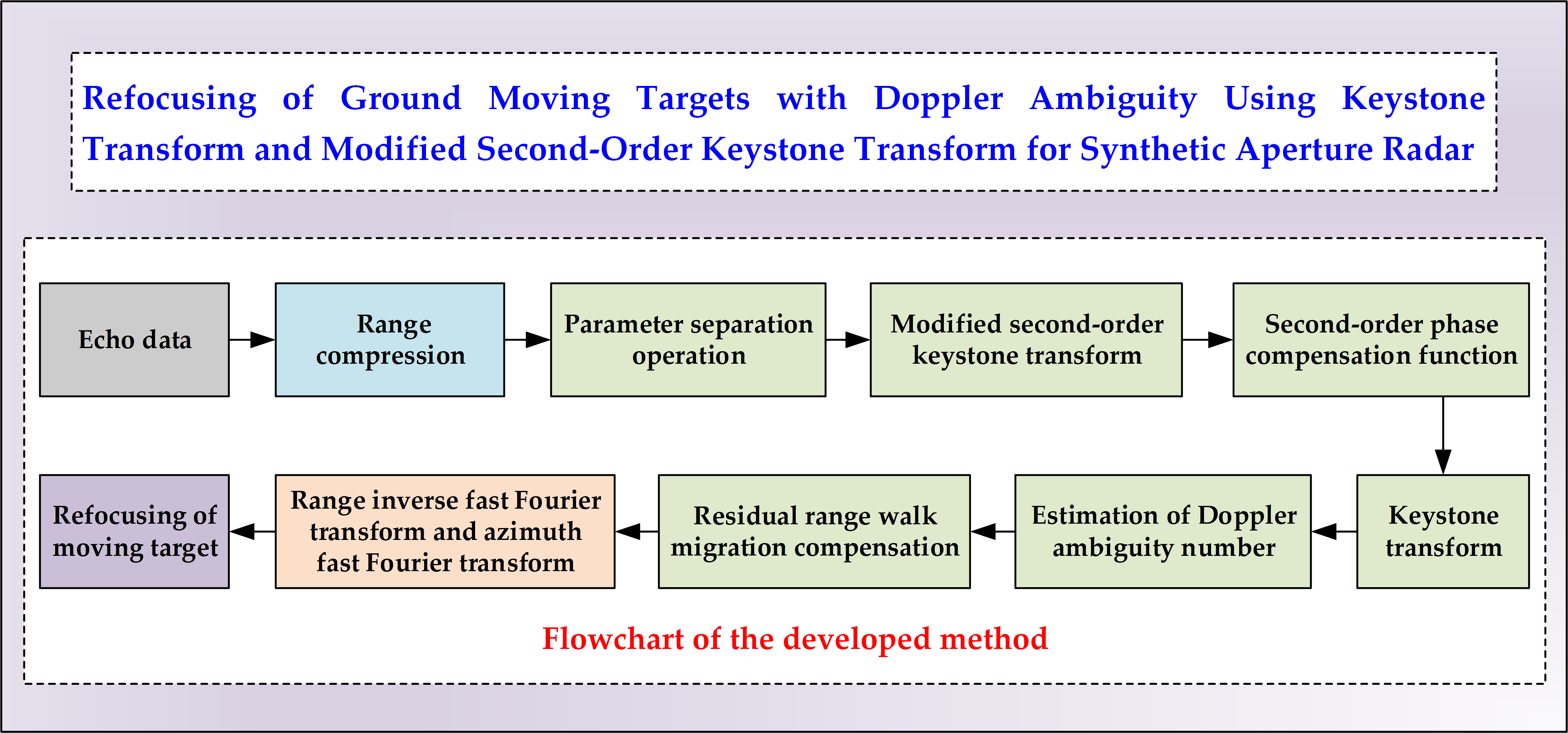
3. Description of the Proposed Algorithm

3.1. Proposed Algorithm

According to Equation (9), the first-order phase parameter is coupled with the second-order phase parameter. This factor will lead to difficulty in the moving target refocusing. Therefore, the parameter separation operation on the basis of time reversing process in the range-frequency and azimuth-time domain is initially utilized as follows:

$$\begin{array}{c}{s}_3(f,t_n)=s_2(f,t_n)s_2(f,{\overleftarrow{t}}_n)\\ =\mathrm{rect}\left(\frac{f}{B}\right)\exp \left[-\frac{j8\pi }{c}(f+f_c)(R_0+{\rho }_2{t}_n^2)\right]\end{array}$$

(10)

where “$\leftarrow$” indicates the azimuth-time reversing process in the range-frequency domain and $s_2(f,{\overleftarrow{t}}_n)=s_2(f,-t_n)$ [30,31,32].

After the parameter separation operation is performed to Equation (9), the coupling between first-order term and second-order term is effectively removed. In accordance with Equation (10), the effect of the first-order term is accurately eliminated. Nevertheless, the second-order term still exists, and the effects of RCM and DFM remain. SOKT is often utilized in traditional methods [22,23] to remove RCM. However, only RCM can be removed by SOKT, and the energy of moving targets still defocuses due to the effect of DFM. In addition, if SOKT is directly used in the presence of Doppler spectrum split, the trajectory of moving targets will be divided into several parts, leading to severe integration loss. Considering that RCM and DFM present in Equation (10), we adopt MSOKT for simultaneously correcting RCM and DFM and estimating the second-order phase coefficient ${\rho }_2$. The detailed expression of MSOKT can be represented as follows [12]:

$$\beta (f+f_c)t_n^2=f_c\xi$$

(11)

where $\beta$ denotes the zoom factor of MSOKT and $\xi$ indicates the scaled time after performing MSOKT. The selection criteria of zoom factor $\beta$ are expounded in Appendix A.

After Equation (11) is substituted into Equation (10), we have:

$$s_3(f,\xi )=\mathrm{rect}\left(\frac{f}{B}\right)\exp \left[-\frac{j8\mathsf{\pi }}{c}\left(f+f_c\right)R_0\right]\exp \left(-\frac{j8\mathsf{\pi }{f}_c{\rho }_2\xi }{c\beta }\right)$$

(12)

Subsequently, Equation (12) is transformed into the range-time and azimuth-scaled frequency domain as follows:

$$s_3\left(t,f_{\xi }\right)=\mathrm{s}\mathrm{i}\mathrm{n}\mathrm{c}\left[B\left(t-\frac{4R_0}{c}\right)\right]\delta \left(f_{\xi }+\frac{4f_c{\rho }_2}{c\beta }\right)$$

(13)

where $f_{\xi }$ indicates the azimuth-scaled frequency variable related to the scaled time $\xi$.

On the basis of Equation (13), the estimated result of the second-order phase coefficient ${\rho }_2$ can be obtained as:

$${\widehat{\rho }}_2=-c\beta {\widehat{f}}_{\xi }/\left(4f_c\right)$$

(14)

In accordance with the estimated ${\widehat{\rho }}_2$, the second-order phase correction function can be constructed as follows:

$$H_1({\widehat{\rho }}_2;f,t_n)=\exp \left[-\frac{j4\mathsf{\pi }}{c}\left(f+f_c\right)\frac{c\beta {\widehat{f}}_{\xi }}{4f_c}{t}_n^2\right]$$

(15)

After Equation (9) is multiplied by Equation (15), it yields:

$$\begin{array}{l}{s}_4(f,t_n)=s_2\left(f,t_n\right)H_1({\widehat{\rho }}_2;f,t_n)\\ =\mathrm{rect}\left(\frac{f}{B}\right)\exp \left[\frac{j4\pi f}{c}\left(k_{\mathrm{a}}\frac{\lambda \mathrm{PRF}}{2}{t}_n\right)\right]\exp \left[-\frac{j4\pi }{c}\left(f+f_{\mathrm{c}}\right)R_0\right]\\ \times \exp \left[\frac{j4\pi }{c}\left(f+f_{\mathrm{c}}\right)v_0{t}_n\right]\hfill \end{array}$$

(16)

As described in Equation (16), the Doppler spectrum split can be avoided given that the effect of DFM is effectively removed by the correction function in Equation (15). This time, KT can be directly utilized to remove RWM without the influence of the target trajectory split. Thereafter, in the following, KT, i.e., $\left(f+f_{\mathrm{c}}\right)t_n=f_{\mathrm{c}}{\eta }_n$ [19], is performed to Equation (16) for correcting RWM, and we have:

$$\begin{array}{ll}{s}_4(f,{\eta }_n)& =\mathrm{rect}\left(\frac{f}{B}\right)\exp \left[-\frac{j4\pi }{c}\left(f+f_{\mathrm{c}}\right)R_0\right]\exp \left(\frac{j4\pi f_{\mathrm{c}}}{c}{v}_0{\eta }_n\right)\\ & \times \exp \left[\frac{j2\pi k_{\mathrm{a}}\mathrm{PRF}f}{\left(f+f_{\mathrm{c}}\right)}{\eta }_n\right]\end{array}$$

(17)

In accordance with Equation (17), though RWM caused by baseband velocity $v_0$ is accurately compensated by using KT, the residual RWM induced by the Doppler ambiguity number still remains. If no residual RWM correction occurs during the subsequent processing steps, the energy of moving target will spread along the range-time dimension, resulting in a serious defocusing effect.

Therefore, on the basis of the last exponential term of Equation (17), the residual RWM correction function is constructed as follows:

$$H_2({\widehat{k}}_{\mathrm{a}};f,{\eta }_n)=\exp \left[-\frac{j2\pi {\widehat{k}}_{\mathrm{a}}\mathrm{PRF}f}{\left(f+f_{\mathrm{c}}\right)}{\eta }_n\right]$$

(18)

where ${\widehat{k}}_{\mathrm{a}}$ denotes the matched Doppler ambiguity number of the residual RWM correction in Equation (18).

After Equation (17) is multiplied by Equation (18), we have:

$$\begin{array}{ll}{s}_5(f,{\eta }_n)& =s_4(f,{\eta }_n)H_2({\widehat{k}}_{\mathrm{a}};f,{\eta }_n)\\ & =\mathrm{rect}\left(\frac{f}{B}\right)\exp \left[-\frac{j4\pi }{c}\left(f+f_{\mathrm{c}}\right)R_0\right]\exp \left(\frac{j4\pi f_{\mathrm{c}}}{c}{v}_0{\eta }_n\right)\\ & \times \exp \left[\left(k_{\mathrm{a}}-{\widehat{k}}_{\mathrm{a}}\right)\frac{j2\pi \mathrm{PRF}f}{\left(f+f_{\mathrm{c}}\right)}{\eta }_n\right]\end{array}$$

(19)

If $k_{\mathrm{a}}={\widehat{k}}_{\mathrm{a}}$ is satisfied, the residual RWM will be effectively removed. Then, Equation (19) can be simplified as follows:

$$s_6(f,{\eta }_n)=\mathrm{rect}\left(\frac{f}{B}\right)\exp \left[-\frac{j4\pi }{c}\left(f+f_{\mathrm{c}}\right)R_0\right]\exp \left(\frac{j4\pi f_{\mathrm{c}}}{c}{v}_0{\eta }_n\right)$$

(20)

After the rang inverse FFT (IFFT) and azimuth FFT are conducted to Equation (20), the moving target can be refocused as follows:

$$s_6(t,f_d)=\mathrm{sinc}\left[B\left(t-\frac{2R_0}{c}\right)\right]\mathrm{s}\mathrm{i}\mathrm{n}\mathrm{c}\left[T_i\left(f_d-\frac{f_{\mathrm{c}}2v_0}{c}\right)\right]$$

(21)

where $f_d$ denotes the frequency variable related to ${\eta }_n$.

Generally, the Doppler ambiguity number $k_{\mathrm{a}}$ of the moving target is priori unknown. In order to focus the moving target, the $k_{\mathrm{a}}$ should be effectively estimated. Therefore, on the basis of Equation (19), the estimation operation of $k_{\mathrm{a}}$ can be defined as follows:

$${\stackrel{⌢}{k}}_{\mathrm{a}}=\underset{{\widehat{k}}_{\mathrm{a}}}{\mathrm{a}\mathrm{r}\mathrm{g}\mathrm{m}\mathrm{a}\mathrm{x}}\left|{\mathrm{FFT}}_{{\eta }_n}\left\{{\mathrm{IFFT}}_f\left[s_4(f,{\eta }_n)H_2({\widehat{k}}_{\mathrm{a}};f,{\eta }_n)\right]\right\}\right|$$

(22)

where ${\stackrel{⌢}{k}}_{\mathrm{a}}$ denotes the estimated result of $k_{\mathrm{a}}$ and the arguments of the maxima is denoted by $\mathrm{argmax}\left(\cdot \right)$. In Equation (22), ${\mathrm{FFT}}_{{\eta }_n}\left(\cdot \right)$ and ${\mathrm{IFFT}}_f\left(\cdot \right)$ indicate the FFT operation along ${\eta }_n$ and the IFFT operation along $f$, respectively.

As shown in Equation (21), a well-refocused result can be achieved by using the proposed method given that the effects of RM, DCS and DFM are effectively eliminated.

According to the above analysis, the flowchart of the developed method is presented in Figure 2.

3.2. Multiple Target Processing Analysis

In this section, the case of multiple target refocusing is discussed. In this case, the target signal in Equation (9) can be rewritten as follows:

$$\begin{array}{ll}{s}_{\mathrm{m}1}\left(f,t_n\right)& ={\displaystyle \sum _{i=1}^L\mathrm{r}\mathrm{e}\mathrm{c}\mathrm{t}\left(\frac{f}{B}\right)\mathrm{e}\mathrm{x}\mathrm{p}\left[-\frac{j4\pi }{c}\left(f+f_c\right)\left(R_{0i}-v_{0i}{t}_n+{\rho }_{2i}{t}_n^2\right)\right]}\\ & \times \mathrm{e}\mathrm{x}\mathrm{p}\left[\frac{j4\pi f}{c}\right.\left.\left(k_{\mathrm{a}i}\frac{c\mathrm{PRF}}{2f_c}{t}_n\right)\right]\end{array}$$

(23)

where L denotes the number of moving targets and $R_{0i}$, $v_{0i}$, ${\rho }_{2i}$, and $k_{\mathrm{a}i}$ represent the nearest slant range, baseband velocity, second-order phase coefficient and Doppler ambiguity number of the ith moving target, respectively.

After the parameter separation operation in Equation (10) is performed to Equation (23), we have:

$$\begin{array}{c}{s}_{\mathrm{m}2}\left(f,t_n\right)=\underset{\mathrm{auto}\text{-}\mathrm{terms}}{\underbrace{{\displaystyle \sum _{i=1}^L}\mathrm{r}\mathrm{e}\mathrm{c}\mathrm{t}\left(\frac{f}{B}\right)\mathrm{e}\mathrm{x}\mathrm{p}\left[-j\frac{8\pi }{c}\left(f+f_c\right){\rho }_{2i}{t}_n^2\right]\mathrm{e}\mathrm{x}\mathrm{p}\left[-j\frac{8\pi }{c}\left(f+f_c\right)R_{0i}\right]}}\\ +{\displaystyle \sum _{i=1}^L}{\displaystyle \sum _{j=1,i\ne j}^L\mathrm{r}\mathrm{e}\mathrm{c}\mathrm{t}\left(\frac{f}{B}\right)}\mathrm{e}\mathrm{x}\mathrm{p}\left[-j\frac{4\pi }{c}\left(f+f_c\right)\left(R_{0i}+R_{0j}\right)\right]\\ \times \mathrm{e}\mathrm{x}\mathrm{p}\left[-j\frac{4\pi }{c}\left(f+f_c\right)\left({\rho }_{2i}+{\rho }_{2j}\right)t_n^2\right]\mathrm{e}\mathrm{x}\mathrm{p}\left[j\frac{4\pi }{c}\left(f+f_c\right)\left(v_{0i}+v_{0j}\right)t_n\right]\\ \underset{\mathrm{cross}\text{-}\mathrm{terms}}{\underbrace{\times \mathrm{e}\mathrm{x}\mathrm{p}\left\{\frac{j4\pi f}{c}\right[\left(k_{\mathrm{a}i}-k_{\mathrm{a}j}\right)\frac{c\mathrm{PRF}}{2f_c}{t}_n\left]\right\}}}\end{array}$$

(24)

According to Equation (24), with regard to the auto-terms, the effects of first-order term (i.e., RWM and DCS) are accurately removed, and only the effects of second-order term (i.e., RCM and DFM) remain. Considering that the cross-track velocities of different moving targets are usually different, $v_{0i}\ne v_{0j}$ or $k_{\mathrm{a}i}\ne k_{\mathrm{a}j}$ can be generally held. With regard to the cross-terms, the effects of first- and second-order terms all remain. Therefore, not only RWMs and DCSs, but also RCMs and DFMs of the cross-terms still exist. Under this case (i.e., $v_{0i}\ne v_{0j}$ or $k_{\mathrm{a}i}\ne k_{\mathrm{a}j}$), MSOKT ($\beta (f+f_c)t_n^2=f_c\xi$) is applied to Equation (24), and yields:

$$\begin{array}{ll}{s}_{\mathrm{m}2}\left(f,\xi \right)& =\underset{\mathrm{auto}\text{-}\mathrm{terms}}{\underbrace{{\displaystyle \sum _{i=1}^L}\mathrm{r}\mathrm{e}\mathrm{c}\mathrm{t}\left(\frac{f}{B}\right)\mathrm{e}\mathrm{x}\mathrm{p}\left[-j\frac{8\pi }{c}\left(f+f_c\right)R_{0i}\right]\mathrm{e}\mathrm{x}\mathrm{p}\left(-j\frac{8\pi f_c{\rho }_{2i}\xi }{c\beta }\right)}}\\ & +{\displaystyle \sum _{i=1}^L{\displaystyle \sum _{j=1,i\ne j}^L\mathrm{r}\mathrm{e}\mathrm{c}\mathrm{t}\left(\frac{f}{B}\right)}}\mathrm{e}\mathrm{x}\mathrm{p}\left[-j\frac{4\pi }{c}\left(f+f_c\right)\left(R_{0i}+R_{0j}\right)\right]\\ & \times \mathrm{e}\mathrm{x}\mathrm{p}\left[-j\frac{4\pi f_c({\rho }_{2i}+{\rho }_{2j})\xi }{c\beta }\right]\mathrm{e}\mathrm{x}\mathrm{p}\left[j\frac{4\pi }{c}\left(v_{0i}+v_{0j}\right){\left[\frac{(f+f_c)f_c\xi }{\beta }\right]}^{\frac{1}{2}}\right]\\ & \underset{\mathrm{cross}\text{-}\mathrm{terms}}{\underbrace{\times \mathrm{e}\mathrm{x}\mathrm{p}\left\{\frac{j4\pi f}{c}\right[\left(k_{\mathrm{a}i}-k_{\mathrm{a}j}\right)\frac{c\mathrm{PRF}}{2f_c}{\left[\frac{f_c\xi }{\beta (f+f_c)}\right]}^{\frac{1}{2}}\left]\right\}}}\end{array}$$

(25)

As shown in Equation (25), after performing MSOKT, the RMs and DFMs of auto-terms are effectively removed. Therefore, the auto-terms can be accumulated as the clear peaks, and the second-order phase coefficients of auto-terms can be correctly estimated. Considering that the second-order phase correction function in Equation (15), KT and the estimation operation of $k_{\mathrm{a}}$ are linear processing steps, the moving targets can be refocused by using the parameters estimated from auto-terms. However, the cross-terms are typically defocused in Equation (25) given that the effects of first-order terms for cross-terms still exist. To summarize, the cross-terms in Equation (25) may not affect the proposed method used for the refocusing of multiple moving targets in this case (i.e., $v_{0i}\ne v_{0j}$ or $k_{\mathrm{a}i}\ne k_{\mathrm{a}j}$).

However, with regard to a particular situation, the moving targets may have the same baseband cross-track velocities and Doppler ambiguity numbers (i.e., $v_{0i}=v_{0j}$ or $k_{\mathrm{a}i}=k_{\mathrm{a}j}$). Under this situation, the signal in Equation (25) can be simplified as follows:

$$\begin{array}{c}{s}_{\mathrm{m}2}(f,\xi )=\underset{\mathrm{auto}\text{-}\mathrm{terms}}{\underbrace{{\displaystyle \sum _{i=1}^L\mathrm{r}\mathrm{e}\mathrm{c}\mathrm{t}\left(\frac{f}{B}\right)}\mathrm{e}\mathrm{x}\mathrm{p}\left[-j\frac{8\pi }{c}\left(f+f_c\right)R_{0i}\right]\mathrm{e}\mathrm{x}\mathrm{p}\left(-j\frac{8\pi f_c{\rho }_{2i}\xi }{c\beta }\right)}}\\ \underset{\mathrm{cross}\text{-}\mathrm{terms}}{\underbrace{\begin{array}{c}+{\displaystyle \sum _{i=1}^L{\displaystyle \sum _{j=1,i\ne j}^L\mathrm{r}\mathrm{e}\mathrm{c}\mathrm{t}\left(\frac{f}{B}\right)}}\mathrm{e}\mathrm{x}\mathrm{p}\left[-j\frac{4\pi }{c}\left(f+f_c\right)\left(R_{0i}+R_{0j}\right)\right]\\ \times \mathrm{e}\mathrm{x}\mathrm{p}\left[-j\frac{4\pi f_c\left({\rho }_{2i}+{\rho }_{2j}\right)\xi }{c\beta }\right]\hfill \end{array}}}\end{array}$$

(26)

Then, Equation (26) can be transformed into the range-time and azimuth-scaled frequency domain as follows:

$$\begin{array}{c}{s}_{\mathrm{m}2}(t,f_{\xi })=\underset{\mathrm{auto}\text{-}\mathrm{terms}}{\underbrace{{\displaystyle \sum _{i=1}^L\mathrm{sinc}\left[B\left(t-\frac{4R_{0i}}{c}\right)\right]\delta \left(f_{\xi }+\frac{4f_c{\rho }_{2i}}{c\beta }\right)}}}\\ \underset{\mathrm{cross}\text{-}\mathrm{terms}}{\underbrace{+{\displaystyle \sum _{i=1}^L{\displaystyle \sum _{j=1,i\ne j}^L\mathrm{sinc}\left[B\left(t-\frac{2R_{0i}+2R_{0j}}{c}\right)\right]\delta \left[f_{\xi }+\frac{2f_c\left({\rho }_{2i}+{\rho }_{2j}\right)}{c\beta }\right]}}}}\end{array}$$

(27)

As described in Equation (27), both the auto- and cross-terms are accumulated as the obvious peaks. The peak positions of auto- and cross-terms can be written as ${\widehat{f}}_{\xi ,i,\mathrm{a}}=-4f_c{\rho }_{2i}/(c\beta )$ and ${\widehat{f}}_{\xi ,i,j,\mathrm{c}}=-2f_c({\rho }_{2i}+{\rho }_{2j})/c\beta$, respectively. Therefore, the second-order phase coefficients estimated from auto- and cross-terms can be, respectively, denoted as follows:

$${\widehat{\rho }}_{2,i,a}=-\frac{c\beta {\widehat{f}}_{\xi ,i,\mathrm{a}}}{4f_c}={\rho }_{2i}\mathrm{and}{\widehat{\rho }}_{2,i,j,\mathrm{c}}=-\frac{c\beta {\widehat{f}}_{\xi ,i,j,\mathrm{c}}}{2f_c}={\rho }_{2i}+{\rho }_{2j}$$

(28)

According to Equation (28), the second-order phase coefficients estimated from the auto-terms may be unaffected by the cross-terms. However, the cross-terms will lead to the spurious peaks and false estimated results of the second-order phase coefficient. Then, the second-order phase coefficients estimated from auto- and cross-terms are, respectively, used to construct the second-order phase correction function in Equation (15), and the corresponding results can be written as follows:

$$H_1({\widehat{\rho }}_{2,i,a};f,t_n)=\exp \left[\frac{j4\mathsf{\pi }}{c}\left(f+f_c\right){\rho }_{2i}{t}_n^2\right]$$

(29)

$$H_1({\widehat{\rho }}_{2,i,j,\mathrm{c}};f,t_n)=\exp \left[\frac{j4\mathsf{\pi }}{c}(f+f_c)({\rho }_{2i}+{\rho }_{2j})t_n^2\right]$$

(30)

After Equation (29) is substituted into Equation (16), we have:

$$\begin{array}{ll}{s}_{\mathrm{m}4\mathrm{a}}(f,t_n)& =s_{\mathrm{m}1}\left(f,t_n\right)H_1({\widehat{\rho }}_{2,i,a};f,t_n)\\ & =\mathrm{r}\mathrm{e}\mathrm{c}\mathrm{t}\left(\frac{f}{B}\right)\mathrm{e}\mathrm{x}\mathrm{p}\left[-\frac{j4\pi }{c}\left(f+f_c\right)\left(R_{0i}-v_{0i}{t}_n\right)\right]\\ & \times \mathrm{e}\mathrm{x}\mathrm{p}\left[\frac{j4\pi f}{c}\right.\left.\left(k_{\mathrm{a}i}\frac{c\mathrm{PRF}}{2f_c}{t}_n\right)\right]\end{array}$$

(31)

where $i=1,\cdots ,L$. According to Equations (17), (18) and (19), after KT and residual RWM correction functions in Equation (18) are performed to Equation (31), we have:

$$s_{\mathrm{m}6\mathrm{a}}(f,{\eta }_n)=\mathrm{rect}\left(\frac{f}{B}\right)\exp \left[-\frac{j4\pi }{c}\left(f+f_{\mathrm{c}}\right)R_{0i}\right]\exp \left(\frac{j4\pi f_{\mathrm{c}}}{c}{v}_{0i}{\eta }_n\right)$$

(32)

As shown in Equation (32), the RMs and DFMs of moving targets are effectively removed by using the second-order phase coefficients estimated from the auto-terms. After performing the range IFFT and azimuth FFT, the moving targets can be refocused.

With regard to the second-order phase coefficients estimated from the cross-terms, after Equation (30) is substituted into Equation (16) it yields:

$$\begin{array}{ll}{s}_{\mathrm{m}4\mathrm{c}}(f,t_n)& =s_{\mathrm{m}1}\left(f,t_n\right)H_1({\widehat{\rho }}_{2,i,j,\mathrm{c}};f,t_n)\\ & =\mathrm{r}\mathrm{e}\mathrm{c}\mathrm{t}\left(\frac{f}{B}\right)\mathrm{e}\mathrm{x}\mathrm{p}\left[-\frac{j4\pi }{c}\left(f+f_c\right)\left(R_{0i}-v_{0i}{t}_n-{\rho }_{2j}{t}_n^2\right)\right]\\ & \times \mathrm{e}\mathrm{x}\mathrm{p}\left[\frac{j4\pi f}{c}\right.\left.\left(k_{\mathrm{a}i}\frac{c\mathrm{PRF}}{2f_c}{t}_n\right)\right]\end{array}$$

(33)

According to Equations (17), (18) and (19), after KT is applied to Equation (33) and the Doppler ambiguity number is correctly matched, the corresponding result can be written as follows:

$$\begin{array}{c}{s}_{\mathrm{m}6\mathrm{c}}(f,{\eta }_n)=\mathrm{r}\mathrm{e}\mathrm{c}\mathrm{t}\left(\frac{f}{B}\right)\mathrm{e}\mathrm{x}\mathrm{p}\left[-\frac{j4\pi }{c}\left(f+f_c\right)R_{0i}\right]\\ \times \mathrm{e}\mathrm{x}\mathrm{p}\left(\frac{j4\pi f_c}{c}{v}_{0i}{\eta }_n\right)\mathrm{e}\mathrm{x}\mathrm{p}\left[\frac{j4\pi f_c^2}{c\left(f+f_{\mathrm{c}}\right)}{\rho }_{2j}{\eta }_n^2\right]\end{array}$$

(34)

where $j=1,\cdots ,L,j\ne i$. As displayed in Equation (34), the effects of the second-order phase still remain. The moving targets are still defocused. Therefore, the false second-order phase coefficients estimated from the cross-terms are used to construct the correction function in Equation (15), and the refocused results in Equation (21) are absent. That is to say, only the second-order phase coefficients estimated from the auto-terms are utilized to construct the correction function in Equation (15), and the final refocused results in Equation (21) can be obtained. Thus, on the basis of this phenomenon, the false second-order phase coefficients estimated from the cross-terms can be identified and the spurious peaks can be rejected.

In summary, in accordance with the above analysis, the proposed method can be used to focus multiple moving targets.

In the following, two simulation examples without background noise are provided to verify the above analysis of multiple target refocusing and spurious peak recognition procedure. The main simulation parameters of radar are set as follows: $f_c=10$ GHz, $B=200$ MHz, $\mathrm{PRF}=1000$ Hz, and $T_i=2$ s. $\beta =4$ is set in the following experiments.

With regard to simulation example A, two moving target signals with different phase parameters are set for simplicity and are denoted by T1 and T2. The main phase parameters of T1 and T2 are set as follows: ${\rho }_{1\mathrm{T}1}=27\mathrm{m}/\mathrm{s}$ and ${\rho }_{2\mathrm{T}1}={1.5\mathrm{m}/\mathrm{s}}^2$ for T1, and ${\rho }_{1\mathrm{T}2}=-18\mathrm{m}/\mathrm{s}$ and ${\rho }_{2\mathrm{T}2}{=3\mathrm{m}/\mathrm{s}}^2$ for T2.

Figure 3 exhibits the results of simulation example A. The range compression results of T1 and T2 are shown in Figure 3a. Two curved trajectories with respect to T1 and T2 are depicted in Figure 3a. Figure 3b shows the result of the parameter separation operation in Equation (10). Not only trajectories of auto-terms, but also trajectories of cross-terms are found in Figure 3b because the parameter separation operation in Equation (10) includes nonlinear operation. As presented in Figure 3b, the RWMs and DCSs of auto-terms are effectively removed, and only the RCMs and DFMs of auto-terms remain. However, for the cross-terms, both the effects of first- and second-order terms (RWM, DCS, RCM and DFM) remain. As displayed in Figure 3c, after MSOKT is used to remove RCM and DFM, the auto-terms are accumulated as two clear peaks, but the evident peaks related to the cross-terms are absent due to the defocusing effect. Therefore, under this situation, the cross-terms do not affect the estimated results of the second-order phases of auto-terms. With the second-order phases estimated from auto-term peaks in Figure 3c, the corresponding phase correction function in Equation (15) is constructed. After the phase correction function in Equation (15) and KT are performed, the estimated results of the Doppler ambiguity numbers of T1 and T2 are obtained, as shown in Figure 3d. After the residual RWM is removed by using the estimated Doppler ambiguity number, the well-refocused results are achieved, and the corresponding results are exhibited in Figure 3e,f.

With regard to simulation example B, two moving target signals, denoted by T3 and T4, with the same first-order phase parameters are considered. The main phase parameters of T3 and T4 are set as follows: ${\rho }_{1\mathrm{T}3}=27\mathrm{m}/\mathrm{s}$ and ${\rho }_{2\mathrm{T}3}={1.5\mathrm{m}/\mathrm{s}}^2$ for T3, and ${\rho }_{1\mathrm{T}4}=27\mathrm{m}/\mathrm{s}$ and ${\rho }_{2\mathrm{T}4}{=3\mathrm{m}/\mathrm{s}}^2$ for T4.

The results of simulation example B are depicted in Figure 4. After range compression, the obtained results of T3 and T4 are shown in Figure 4a. Two target trajectories related to T3 and T4 are found in Figure 4a. After the parameter separation operation in Equation (10) is applied, the corresponding result is displayed in Figure 4b. According to the analysis in Section 3.2, because the first-order term of T3 is the same as that of T4 (i.e., ${\rho }_{1\mathrm{T}3}={\rho }_{1\mathrm{T}4}$), not only the RWMs and DCSs of auto-terms, but also the RWMs and DCSs of cross-terms are removed. Both the RCMs and DFMs of auto- and cross-terms remain. Therefore, after MSOKT is used, not only the auto-terms, but also the cross-terms are accumulated as clear peaks, denoted by Auto-term A, Auto-term B, and Cross-term A, as shown in Figure 4c. Therefore, under this case, according to the peak positions, the three estimated results of the second-order phases are obtained. On the basis of the results in Figure 4c, the second-order phase coefficients estimated from the auto-terms are unaffected by the cross-terms. However, the cross-terms result in the spurious peaks. According to the magenta and blue lines in Figure 4d, with the second-order phase coefficients estimated from the peaks Auto-term A and Auto-term B and KT, two clear peaks with respect to T3 and T4 are obtained. Then, the Doppler ambiguity numbers of T3 and T4 are estimated based on the peaks in Figure 4d. However, in accordance with the black line in Figure 4d, with the second-order phase coefficient estimated from the peak Cross-term A and KT, the obvious peak is absent. Therefore, the peak Cross-term A is confirmed as a spurious peak and the second-order phase coefficient estimated from peak Cross-term A is a false result. Thus, we can use the result in Figure 4d to identify the spurious peaks. After the residual RWM is compensated by using the estimated Doppler ambiguity number, the corresponding well-refocused results of T3 and T4 are achieved and displayed in Figure 4e,f.

In summary, the above simulation results verify that the spurious peaks can be identified by the proposed processing strategy of cross-terms. Therefore, the presented method can be utilized to refocus multiple targets.

4. Simulation Experimental Results

The results of simulation experiment in the presence of Gaussian background are provided to demonstrate the effectiveness of the proposed method.

The basic parameters of simulation radar are summarized in

Table 1. Basic parameters of simulation radar.

Parameters	Value
Carrier frequency	10 GHz
Range bandwidth	200 MHz
Pulse repetition frequency	1000 Hz
Radar platform velocity	120 m/s
Nearest slant range	5000 m
Integration time	2s

. Three moving targets, indicated by Target 1, Target 2 and Target 3, are set in this simulation experiment. The main simulation parameters of three moving targets are presented in

Table 2. Simulation parameters of three moving targets.

	Cross-Track Velocity (m/s)	Along-Track Velocity (m/s)
Target 1	26	16
Target 2	−11	−30
Target 3	12	−10

. The signal-to-noise ratio is set as −13 dB. Target 1 and Target 3 are Doppler center blur targets, and their Doppler spectra still occupy one PRF band. Target 2 is a Doppler spectrum split target, and its Doppler spectrum spreads into two PRF bands.

Figure 5 shows the simulation experimental results. The range compression results of three targets are depicted in Figure 5a. Three curved trajectories of Target 1, Target 2 and Target 3 are found in Figure 5a, and these trajectories of targets occupy multiple range bins due to the effect of RM, resulting in severe target energy defocusing. The azimuth Doppler spectrum distributions of Target 1, Target 2 and Target 3 are illustrated in Figure 5b. Notably, the energy of three targets still spans over the azimuth Doppler frequency domain given the effect of DFM, which leads to serious defocusing. Additionally, the target azimuth spectra of Target 1 and Target 3 distribute into one PRF band, and the target azimuth spectrum of Target 2 occupies two PRF bands. Figure 5c displays the result after applying the parameter separation operation in Equation (10). Then, in order to illustrate the trajectories of three moving targets clearly, the background is removed. As shown in Figure 5c, the RWMs and DCSs of Target 1, Target 2 and Target 3 are accurately eliminated. Only the RCMs and DFMs of Target 1, Target 2 and Target 3 remain. With regard to cross-terms, RWM, RCM and DFM still exist. Figure 5d shows the result after performing MSOKT. Only three obvious peaks with respect to Target 1, Target 2 and Target 3 are exhibited in Figure 5d, and the cross-terms are still defocused, thereby helping to avoid the effects of cross-terms. In accordance with the peak positions in Figure 5d and KT, the estimated results of Doppler ambiguity numbers for Target 1, Target 2 and Target 3 are shown in Figure 5e. After the residual RWMs of Target 1, Target 2 and Target 3 are removed by the corresponding estimated Doppler ambiguity numbers, the well-refocused results of Target 1, Target 2 and Target 3 are presented in Figure 5f,g,h, respectively.

To summarize, the simulation experimental results verify that the developed method can accurately remove RMs and DFMs of multiple moving targets. In addition, the well-refocused result can also be obtained in the presence of Doppler ambiguity (including Doppler center blur and spectrum split).

5. Real Data Processing Results

5.1. Airborne Real Data Processing Result

In the following, a part of airborne real SAR data is presented to confirm the effectiveness of the proposed method. These airborne real SAR data were measured by an X-band three-channel radar wording on a broadside strip-map mode. The main radar parameters are summarized in

Table 3. Main radar parameters for X-band SAR system.

Parameters	Value
Carrier frequency	8.85 GHz
Range bandwidth	40 MHz
Pulse duration time	10 μs
Pulse repetition frequency	1000 Hz

. The pulse number of selected data is set as 3000.

Figure 6a shows the range compression results in the range-Doppler domain. The ground moving targets are submerged by the clutter. Then, the extended factored approach [33] is performed to suppress the strong ground clutter. The result of clutter suppression is displayed in Figure 6b. The processed moving target, indicated by Target A, is highlighted in Figure 6b. Figure 6c exhibits the refocusing result of a selected moving target by using FFT. The moving target still suffers from a defocusing effect due to severe RM and DFM. The estimated result of the second-order phase coefficient of a selected moving target is shown in Figure 6d. With the second-order phase correction function in Equation (15) and KT, the Doppler ambiguity number of the selected moving target is estimated, as shown in Figure 6e. With the estimated Doppler ambiguity number, the remaining RWM is effectively removed, and the final refocused result is obtained. As shown in Figure 6f, a well-refocused result is achieved. Therefore, the above airborne real data processing results verify the effectiveness of the developed method.

5.2. Spaceborne Real Data Processing Result

In this part, the processing results of a part of C-band spaceborne SAR data [5] are presented to verify the effectiveness of the developed method. The measured SAR data are collected by the RADARSAT-1 system. The main parameters of radar are summarized in

Table 4. Main radar parameters for RADARSAR-1.

Parameters	Value
Carrier frequency	5.3 GHz
Range bandwidth	30.116 MHz
Pulse duration time	41.74 μs
Pulse repetition frequency	1256.98 Hz

. The pulse number of processed SAR data is 1200.

Figure 7a shows the range compressed result of the selected spaceborne SAR data. The target trajectories span over several range bins due to serious RM and their energy exhibits severe defocusing phenomena. Figure 7b,c display the estimated result of the second-order phase coefficient and Doppler ambiguity number, respectively. After the remaining RWM is compensated by the estimated Doppler ambiguity number, the final refocused result is depicted in Figure 7d. Then, the processed results of KT, the IAR–TRT method in [13], and the cross-track velocity-searching method in [12] are provided for comparison. The result by directly using KT is shown in Figure 7e. The moving target still suffers from the effect of RM given the Doppler ambiguity. Figure 7f displays the processing result of the cross-track velocity-searching method in [12]. As depicted in Figure 7f, the performance of the method in [12] is deteriorated by the severe BSSL problem. Figure 7g,h show the processing results of the IAR–TRT method in [13]. As exhibited in Figure 7h, the invalid estimated result of the second-order phase coefficient for the IAR–TRT method is obtained given the problem of scaled frequency spectrum aliasing. Compared with the IAR–TRT method, the developed method can deal with the scaled frequency spectrum aliasing effect, and in comparison with the method in [12], the proposed method can avoid the BSSL problem.

6. Discussion

6.1. Computational Cost

In this section, the computational costs of the developed method, the IAR–TRT method in [13] and the cross-track velocity-searching method in [12] are discussed. Similar to [12,13], the computational cost is denoted by the number of complex multiplications. $M$, $N$, $I_{\mathrm{d}}$, $I_1$ and $I_2$ are used to indicate the numbers of range bins, azimuth pluses, searching Doppler ambiguity number, searching first-order phase for the IAR–TRT method and searching first-order phase for the cross-track velocity-searching method in [12]. The main computational costs of the proposed method consist of the operations of MSOKT, KT and the Doppler ambiguity number estimation. Notably, the realization of MSOKT operation can be sped up by nonuniform fast Fourier transform (NUFFT). The detailed description of NUFFT can refer to [34,35,36]. The computational burden of the NUFFT-based MSOKT operation is indicated by $\mathrm{O}(MN\mathrm{l}\mathrm{o}{\mathrm{g}}_2^N)$. Additionally, KT can be implemented without the interpolation [21]. The computational complexity of the interpolation-free-based KT operation is denoted as $\mathrm{O}(MN\mathrm{l}\mathrm{o}{\mathrm{g}}_2^N)$ [21]. Therefore, the main computational complexity of the developed method is represented as $\mathrm{O}[(I_{\mathrm{d}}+2)(MN\mathrm{l}\mathrm{o}{\mathrm{g}}_2^N+NM\mathrm{l}\mathrm{o}{\mathrm{g}}_2^M)]$. With regard to the IAR–TRT method, the main computational cost is obtained using $\mathrm{O}[(I_1+4)MN\mathrm{l}\mathrm{o}{\mathrm{g}}_2^N]$. The main computational complexity of the cross-track velocity-searching method is indicated by $\mathrm{O}[(I_2+1)MN\mathrm{l}\mathrm{o}{\mathrm{g}}_2^N]$. The detailed computational complexities of the above-mentioned methods are summarized in

Table 5. Computational complexities of three methods.

Methods	Computational Complexity
IAR–TRT method [13]	$\mathrm{O}[(I_1+4)MN{\log }_2^N]$
Cross-track velocity-searching method [12]	$\mathrm{O}[(I_2+1)MN{\log }_2^N]$
Proposed method	$\mathrm{O}[(I_{\mathrm{d}}+2)(MN{\log }_2^N+NM{\log }_2^M)]$

. Then, the curves of the computational burden versus the number of azimuth pulses for three methods are exhibited in Figure 8. The results in Table 5 and Figure 8 validate that the computational burdens of the IAR–TRT and cross-track velocity-searching methods are significantly higher than that of the developed method. In addition, the proposed method is computationally efficient because the interpolation operation is free and NUFFT is utilized to speed up the processing step.

6.2. Some Remarks

Remark 1. 

Compared with the IAR–TRT approach [13], the presented method is more robust to scaled frequency spectrum aliasing. The developed method can deal with the BSSL problem in comparison with the cross-track velocity-matching method [12]. The developed method considers the influence of the along-track velocity of ground moving targets and effectively eliminates the effects of RCM and DFM in comparison with the deramp-keystone and stationary phase-based methods [15,16]. In comparison with the traditional KT [19,20,21,29,31], SOKT [22,23] and DKT [24], the presented approach can work well in the presence of Doppler ambiguity (including Doppler center blur and spectrum split). Compared with multi-dimensional searching methods [25,26,27], the computational cost of the proposed method is markedly reduced.

Remark 2. 

The developed method considers the uniform moving target with the second-order model. However, with regard to the highly maneuvering target, the high-order (more than the second-order) model should be considered. In this case, the performance of the proposed method will degrade. In addition, the extremely heterogeneous background is not considered in the proposed approach. Therefore, fast implementation for the refocusing of moving targets with a high-order model in the extremely heterogeneous background is still a challenging task and will be studied in the future.

7. Conclusions

The moving target energy will seriously defocus given that the unknown relative motions between the SAR platform and ground moving targets lead to severe RM and DFM. The low PRF for the SAR system easily makes the signal of ground moving targets show Doppler ambiguity. The RM, DFM and Doppler ambiguity induce the difficulty in refocusing the ground moving targets. In order to address these issues, a SAR ground moving target refocusing method based on KT and MSOKT is developed in this paper. The proposed method can effectively eliminate RM and DFM (containing RWM, RCM, and DFM) and obtain well-refocused results of multiple moving targets in the presence of Doppler ambiguity (containing Doppler center blur and spectrum split) with a low computational cost. The properties of the developed method are summarized as follows: (1) RM and DFM can be accurately removed without the residual compensation errors; (2) the developed approach is robust to Doppler ambiguity; (3) the BSSL problem can be effectively addressed; (4) the interference of cross-term for the multiple moving target case is analyzed, and the corresponding identification strategy of cross-term is presented to recognize the spurious peak; (5) the proposed method can be sped up by NUFFT without the interpolation operation. The effectiveness of the proposed method is confirmed by both airborne and spaceborne real data processing results.

However, the presented approach is unsuitable for refocusing moving targets with a high-order model in the presence of an extremely heterogeneous background. This issue will be addressed in our future work.

References

1. Moreira, A.; Iraola, P.P.; Younis, M.; Krieger, G.; Hajnsek, I.; Papathanassiou, K.P. A tutorial on synthetic aperture radar. IEEE Geosci. Remote Sens. Mag. 2013, 1, 6–43. [Google Scholar] [CrossRef] [Green Version]
2. Filippo, B.; Pia, A.; Danilo, O.; Carmine, C. Micro-motion estimation of maritime targets using pixel tracking in Cosmo-Skymed synthetic aperture radar data-an operative assessment. Remote Sens. 2019, 11, 1637. [Google Scholar]
3. Tang, S.; Zhang, L.; So, H.C. Focusing high-resolution highly-squinted airborne SAR data with maneuvers. Remote Sens. 2018, 10, 8623. [Google Scholar] [CrossRef] [Green Version]
4. Li, X.; Zhou, S.; Yang, L. A new fast factorized back-projection algorithm with reduced topography sensibility for missile-borne SAR focusing with diving movement. Remote Sens. 2020, 12, 2616. [Google Scholar] [CrossRef]
5. Cumming, I.G.; Wong, F.H. Digital Processing of Synthetic Aperture Radar Data: Algorithm and Implementation; Artech House: Norwood, MA, USA, 2005. [Google Scholar]
6. Qin, M.; Li, D.; Tang, X.; Cao, Z.; Li, W.; Xu, L. A fast high-resolution imaging algorithm for helicopter-borne rotating array SAR based on 2-D chirp-z transform. Remote Sens. 2019, 11, 1669. [Google Scholar] [CrossRef] [Green Version]
7. Huang, Y.; Liao, G.; Xu, J.; Li, J.; Yang, D. GMTI and parameter estimation for MIMO SAR system via fast interferometry RPCA method. IEEE Trans. Geosci. Remote Sens. 2018, 56, 1774–1787. [Google Scholar] [CrossRef]
8. Chen, Z.; Zhou, Y.; Zhang, L.; Lin, C.; Huang, Y.; Tang, S. Ground moving target imaging and analysis for near-space hypersonic vehicle-borne synthetic aperture radar system with squint angle. Remote Sens. 2018, 10, 1966. [Google Scholar] [CrossRef] [Green Version]
9. Rahmanizadeh, A.; Amini, J. An integrated method for simulation of synthetic aperture radar (SAR) raw data in moving target detection. Remote Sens. 2017, 9, 1009. [Google Scholar] [CrossRef] [Green Version]
10. Chen, Z.; Zhou, Y.; Zhang, L.; Wei, H.; Lin, C.; Liu, N.; Wan, J. General range model for multi-channel SAR/GMTI with curvilinear flight trajectory. Electron. Lett. 2019, 55, 111–112. [Google Scholar] [CrossRef]
11. Baumgartner, S.V.; Krieger, G. Simultaneous high-resolution wide-swath SAR imaging and ground moving target indication: Processing approaches and system concepts. IEEE J. Sel. Topics Appl. Earth Observ. Remote Sens. 2015, 8, 5015–5029. [Google Scholar] [CrossRef]
12. Wan, J.; Zhou, Y.; Zhang, L.; Chen, Z. Ground moving target focusing and motion parameter estimation method via MSOKT for synthetic aperture radar. IET Signal Process. 2019, 13, 528–537. [Google Scholar] [CrossRef]
13. Huang, P.; Xia, X.G.; Liu, X.; Liao, G. Refocusing and motion parameter estimation for ground moving targets based on improved axis rotation-time reversal transform. IEEE Trans. Comput. Imag. 2018, 4, 479–494. [Google Scholar] [CrossRef]
14. Chen, Z.; Zhang, L.; Zhou, Y.; Lin, C.; Tang, S.; Wan, J. A non-adaptive space-time clutter canceller for multi-channel synthetic aperture radar. IET Signal Process. 2019, 13, 472–479. [Google Scholar] [CrossRef]
15. Sun, G.; Xing, M.; Xia, X.G.; Wu, Y.; Bao, Z. Robust ground moving-target imaging using deramp-Keystone processing. IEEE Trans. Geosci. Remote Sens. 2013, 51, 966–982. [Google Scholar] [CrossRef]
16. Zhu, S.; Liao, G.; Qu, Y.; Zhou, Z.; Liu, X. Ground moving targets imaging algorithm for synthetic aperture radar. IEEE Trans. Geosci. Remote Sens. 2011, 49, 462–477. [Google Scholar] [CrossRef]
17. Zeng, H.; Chen, J.; Wang, P.; Yang, W.; Liu, W. 2-D coherent integration processing and detecting of aircrafts using GNSS-based passive radar. Remote Sens. 2018, 10, 1164. [Google Scholar] [CrossRef] [Green Version]
18. Oveis, A.H.; Sebt, M.A. Coherent method for ground-moving target indication and velocity estimation using Hough transform. IET Radar Sonar Navig. 2017, 11, 646–655. [Google Scholar] [CrossRef]
19. Perry, R.P.; DiPietro, R.C.; Fante, R.L. SAR imaging of moving targets. IEEE Trans. Aerosp. Electron. Syst. 1999, 35, 188–200. [Google Scholar] [CrossRef]
20. Dai, Z.; Zhang, X.; Fang, H.; Bai, Y. High accuracy velocity measurement based on keystone transform using entropy minimization. Chin. J. Electron. 2016, 25, 774–778. [Google Scholar] [CrossRef]
21. Zhu, D.; Li, Y.; Zhu, Z. A keystone transform without interpolation for SAR ground moving-target imaging. IEEE Geosci. Remote Sens. Lett. 2007, 4, 18–22. [Google Scholar] [CrossRef]
22. Kirkland, D. Imaging moving targets using the second-order keystone transform. IET Radar Sonar Navig. 2011, 5, 902–910. [Google Scholar] [CrossRef]
23. Zhou, F.; Wu, R.; Xing, M. Approach for single channel SAR ground moving target imaging and motion parameter estimation. IET Radar Sonar Navig. 2007, 1, 59–66. [Google Scholar] [CrossRef]
24. Li, G.; Xia, X.G.; Peng, Y. Doppler keystone transform: An approach suitable for parallel implementation of SAR moving target imaging. IEEE Geosci. Remote Sens. Lett. 2008, 5, 573–577. [Google Scholar] [CrossRef]
25. Chen, X.; Guan, J.; Liu, N.; Zhou, W.; He, Y. Detection of a low observable sea-surface target with micromotion via Radon-linear canonical transform. IEEE Geosci. Remote Sens. Lett. 2014, 11, 1125–1129. [Google Scholar]
26. Chen, X.; Guan, J.; Liu, N.; He, Y. Maneuvering target detection via Radon-fractional Fourier transform-based long-time coherent integration. IEEE Trans. Signal Process. 2014, 62, 939–953. [Google Scholar] [CrossRef]
27. Li, X.; Cui, G.; Yi, W.; Kong, L. Coherent integration for maneuvering target detection based on Radon-Lv’s distribution. IEEE Signal Process. 2015, 22, 1467–1471. [Google Scholar] [CrossRef]
28. Wan, J.; Chen, Z.; Zhou, Y.; Li, D.; Huang, Y.; Zhang, L. Ground moving target imaging based on MSOKT and KT for synthetic aperture radar. In Proceedings of the IEEE International Geoscience Remote Sensing Symposium, HI, USA, 26 September–2 October 2020; pp. 2141–2144. [Google Scholar]
29. Tian, J.; Cui, W.; Xia, X.G.; Wu, S. Parameter estimation of ground moving targets based on SKT-DLVT processing. IEEE Trans. Comput. Imag. 2016, 2, 13–26. [Google Scholar] [CrossRef] [Green Version]
30. Wu, Y.; So, H.C.; Liu, H. Subspace-based algorithm for parameter estimation of polynomial phase signals. IEEE Trans. Signal Process. 2008, 56, 4977–4983. [Google Scholar]
31. Huang, P.; Liao, G.; Yang, Z.; Xia, X.G.; Ma, J.; Zhang, X. An approach for refocusing of ground moving target without motion parameter estimation. IEEE Trans. Geosci. Remote Sens. 2017, 55, 336–350. [Google Scholar] [CrossRef]
32. Huang, P.; Liao, G.; Yang, Z.; Shu, Y.; Du, W. Approach for space-based radar maneuvering target detection and high-order motion parameter estimation. IET Radar Sonar Navig. 2015, 9, 732–741. [Google Scholar] [CrossRef]
33. DiPietro, R.C. Extended factored space-time processing for airborne radar systems. In Proceedings of the Twenty-Sixth Asilomar Conference on Signals, Systems & Computers, Pacific Grove, CA, USA, 26–28 October 1992; pp. 425–430. [Google Scholar]
34. Liu, Q.H.; Nguyen, N. An accurate algorithm for nonuniform fast Fourier transforms (NUFFT’s). IEEE Microw. Guided Wave Lett. 1998, 8, 18–20. [Google Scholar] [CrossRef]
35. Song, J.Y.; Liu, Q.H.; Torrione, P.; Collins, L. Two-dimensional and three-dimensional NUFFT migration method for landmine detection using ground-penetrating radar. IEEE Trans. Geosci. Remote Sens. 2006, 44, 1462–1469. [Google Scholar] [CrossRef]
36. Liu, Q.H.; Nguyen, N.; Tang, X.Y. Accurate algorithms for nonuniform fast forward and inverse Fourier transforms and their applications. In Proceedings of the IEEE International Geoscience Remote Sensing Symposium, Seattle, DC, USA, 6–10 July 1998; pp. 288–290. [Google Scholar]
Figure 1. Motion geometry configuration between the synthetic aperture radar (SAR) platform and moving target on a slant-rang plane.
Remotesensing 13 00177 g001
Figure 2. Flowchart of the developed method.
Remotesensing 13 00177 g002
Figure 3. Results of simulation example A: (a) Result of range compression. (b) Result of parameter separation operation in Equation (10). (c) Modified second-order keystone transform (MSOKT) result. (d) Estimated result of Doppler ambiguity number. (e) Final refocused result of T1. (f) Final refocused result of T2.
Remotesensing 13 00177 g003
Figure 4. Results of simulation example B: (a) Result of range compression. (b) Result of parameter separation operation in Equation (10). (c) MSOKT result. (d) Estimated result of Doppler ambiguity number. (e) Final refocused result of T3. (f) Final refocused result of T4.
Remotesensing 13 00177 g004
Figure 5. Simulation Experimental Results: (a) Result of range compression of three targets. (b) Azimuth spectrum distributions of three targets. (c) Result of parameter separation operation in Equation (10) of three targets. (d) MSOKT result of three targets. (e) Estimated results of Doppler ambiguity number of three targets. (f) Final refocused result of Target 1. (g) Final refocused result of Target 2. (h) Final refocused result of Target 3.
Remotesensing 13 00177 g005
Figure 6. Airborne real data processing results: (a) Range compression result. (b) Clutter suppression result. (c) Focusing result by direct fast Fourier transform (FFT). (d) Estimated second-order phase coefficient. (e) Estimated result of Doppler ambiguity number. (f) Final refocused result by proposed method.
Remotesensing 13 00177 g006
Figure 7. Spaceborne real data processing results: (a) Range compression result. (b) Estimated second-order phase coefficient by proposed method. (c) Estimated result of Doppler ambiguity number. (d) Final refocused result. (e) Result by direct keystone transform (KT). (f) Result by the method in [12]. (g) Result by the method in [13]. (h) Estimated second-order phase coefficient by the method in [13].
Remotesensing 13 00177 g007aRemotesensing 13 00177 g007b
Figure 8. Curves of computational cost vs. the azimuth pulse number for three methods.
Remotesensing 13 00177 g008