Article

Spatial Temporal Analysis of Traffic Patterns during the COVID-19 Epidemic by Vehicle Detection Using Planet Remote-Sensing Satellite Images

1
Department of Civil, Environmental and Geodetic Engineering, The Ohio State University, Columbus, OH 43210, USA
2
Department of Electrical and Computer Engineering, The Ohio State University, Columbus, OH 43210, USA
3
Translational Data Analytics Institute, The Ohio State University, Columbus, OH 43210, USA
*
Author to whom correspondence should be addressed.
Submission received: 9 December 2020 / Revised: 4 January 2021 / Accepted: 5 January 2021 / Published: 8 January 2021

Abstract

:
The spread of the COVID-19 since the end of 2019 has reached an epidemic level and has quickly become a global public health crisis. During this period, the responses for COVID-19 were highly diverse and decentralized across countries and regions. Understanding the dynamics of human mobility change at high spatial temporal resolution is critical for assessing the impacts of non-pharmaceutical interventions (such as stay-at-home orders, regional lockdowns and travel restrictions) during the pandemic. However, this requires collecting traffic data at scale, which is time-consuming, cost-prohibitive and often not available (e.g., in underdeveloped countries). Therefore, spatiotemporal analysis through processing periodical remote-sensing images is very beneficial to enable efficient monitoring at the global scale. In this paper, we present a novel study that utilizes high temporal Planet multispectral images (from November 2019 to September 2020, on average 7.1 days of frequency) to detect traffic density in multiple cities through a proposed morphology-based vehicle detection method and evaluate how the traffic data collected in such a manner reflect mobility pattern changes in response to COVID-19. Our experiments at city-scale detection, demonstrate that our proposed vehicle detection method over this 3 m resolution data is able to achieve a detection level at an accuracy of 68.26% in most of the images, and the observations’ trends coincide with existing public data of where available (lockdown duration, traffic volume, etc.), further suggesting that such high temporal Planet data with global coverage (although not with the best resolution), with well-devised detection algorithms, can sufficiently provide traffic details for trend analysis to better facilitate informed decision making for extreme events at the global level.

Graphical Abstract

1. Introduction

The coronavirus pandemic in 2019 (COVID-19) [1] emerged as a public health crisis [2]. Various public policies and interventions have been implemented to exercise social distancing [3] to effectively reduce the transmission of COVID-19 [4], such as to reduce human mobility by implementing city and regional lockdowns [5], stay-at-home orders [6,7] and traffic controls [8]. To understand how well these are practiced and their correlations with the COVID-19 impact, existing approaches rely on a large amount of data such as traffic records [9], mobile device signals [10] and social media [11], either collected from public/government databases, or crowdsourcing. However, collecting such resource-rich data is time-consuming and cost-prohibitive. The availability of data is highly unbalanced across different geographical regions, with varying and uncontrolled data quality, for example, data might be more comprehensive in developed countries than in underdeveloped countries. Therefore, in practice, such a study may be region-specific and cannot be scaled at the global level.
Spatiotemporal analysis using remote-sensing satellite images as an alternative, plays an important role to understand the impact of extreme events on a global scale. However, such capability is usually limited due to either the lack of spatial resolution or the lack of temporal resolution of the data, therefore most of the applications were conducted on the landscape level such as for water, snow and urbanization, deforestation, etc. [12,13,14,15]. The recent development of satellite constellations (i.e., Worldview and Planet) can provide high spatial resolution images at a high temporal frequency. In particular, the Planet constellation is capable of leveraging more than 150 small optical satellites to achieve imaging of the global surface at the resolution of 3–5 m with a weekly and even daily revisit rate [16], which has a great potential for applications monitoring objects at a finer scale.
In this work, we propose a novel study that utilizes the high temporal Planet data to understand the traffic patterns and their correlation with COVID-19 which is impacting cities globally. The underlying rationale is to validate the possibility of using such data to infer the human mobility/activities at a very high-temporal resolution at the global scale, such that it can potentially serve as a predictive and objective measure for such events in a timely manner, and at locations where other types of data are not available. To achieve such a goal, firstly, we propose a vehicle detection algorithm for the Planet 3 m resolution multispectral images, and given the relatively low resolution for a small object like cars, our proposed method utilize a morphological top-hat based operator, with the aid of road network layers from OpenStreetMap(OSM) [17] to identify car hotspots, followed by a cascading procedure for post-processing. These car candidates are further turned into traffic density to reflect human mobility on a specific date; secondly, we take our detection algorithm and have practiced the detection at five cities or districts on the downloaded Planet images (on average with a temporal resolution of 7.1 days), and perform trend analysis by correlating the trend resulting from the detected traffic densities with the trend resulting from available statistics on the COVID-19 impact including the traffic lockdown, number of cases, etc. We hypothesize that although the high-temporal Planet data comes with a 3-m resolution barely representing cars with a few pixels, the resulting traffic density statistics from our proposed method can present the general trends showing limited road traffic reflecting the impact of extreme events such as the COVID-19. We consider our work to have the following three contributions:
  • We develop a morphology-based vehicle detection method on the 3-m resolution Planet images with validation for the detection accuracy.
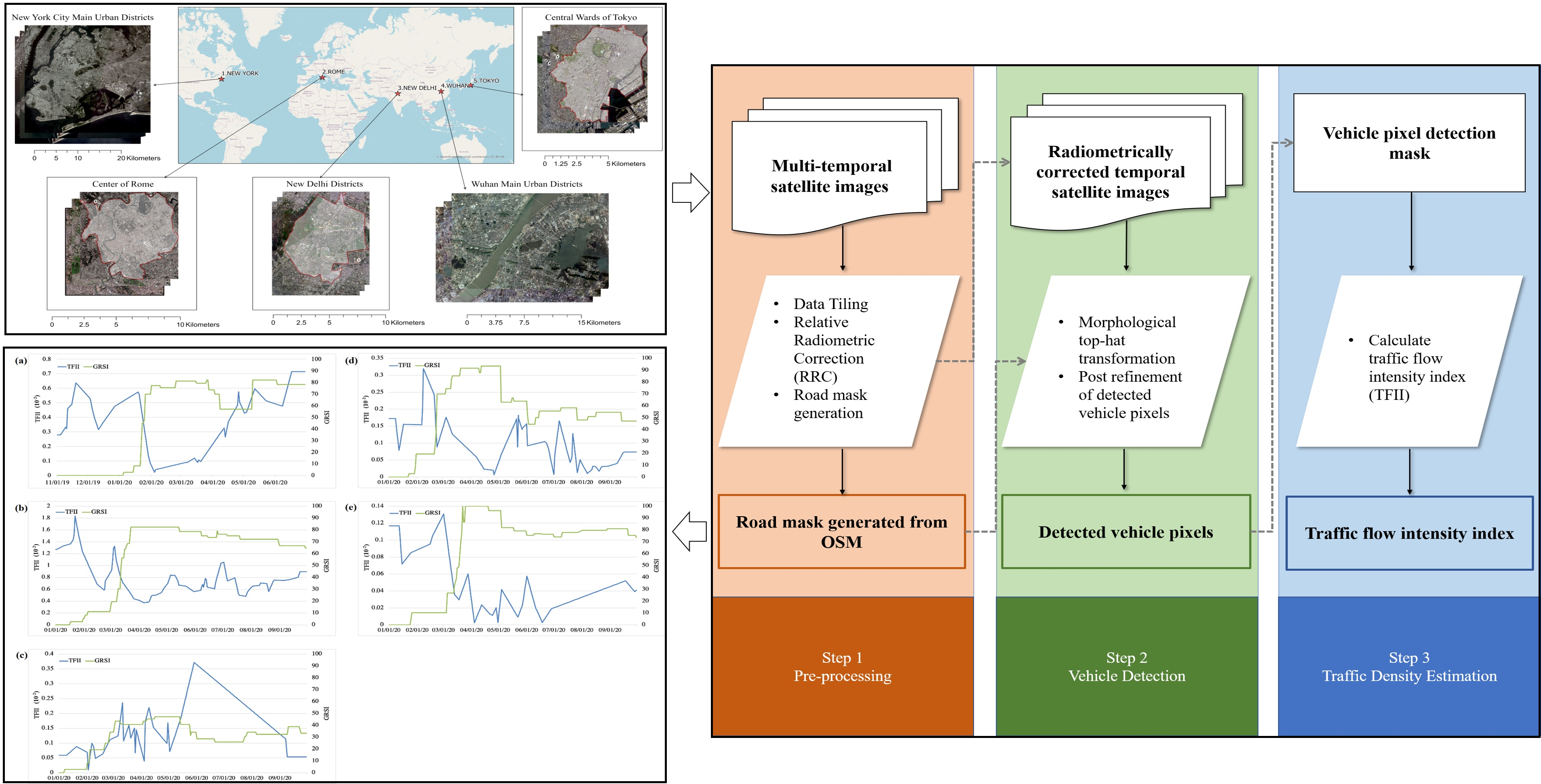
  • Based on our developed method, we generate the traffic density trends for five cities and districts at an average temporal resolution of 7.1 days to offer instrumental insights that low-resolution satellite images can be utilized to estimate traffic intensity at a small geographical scale
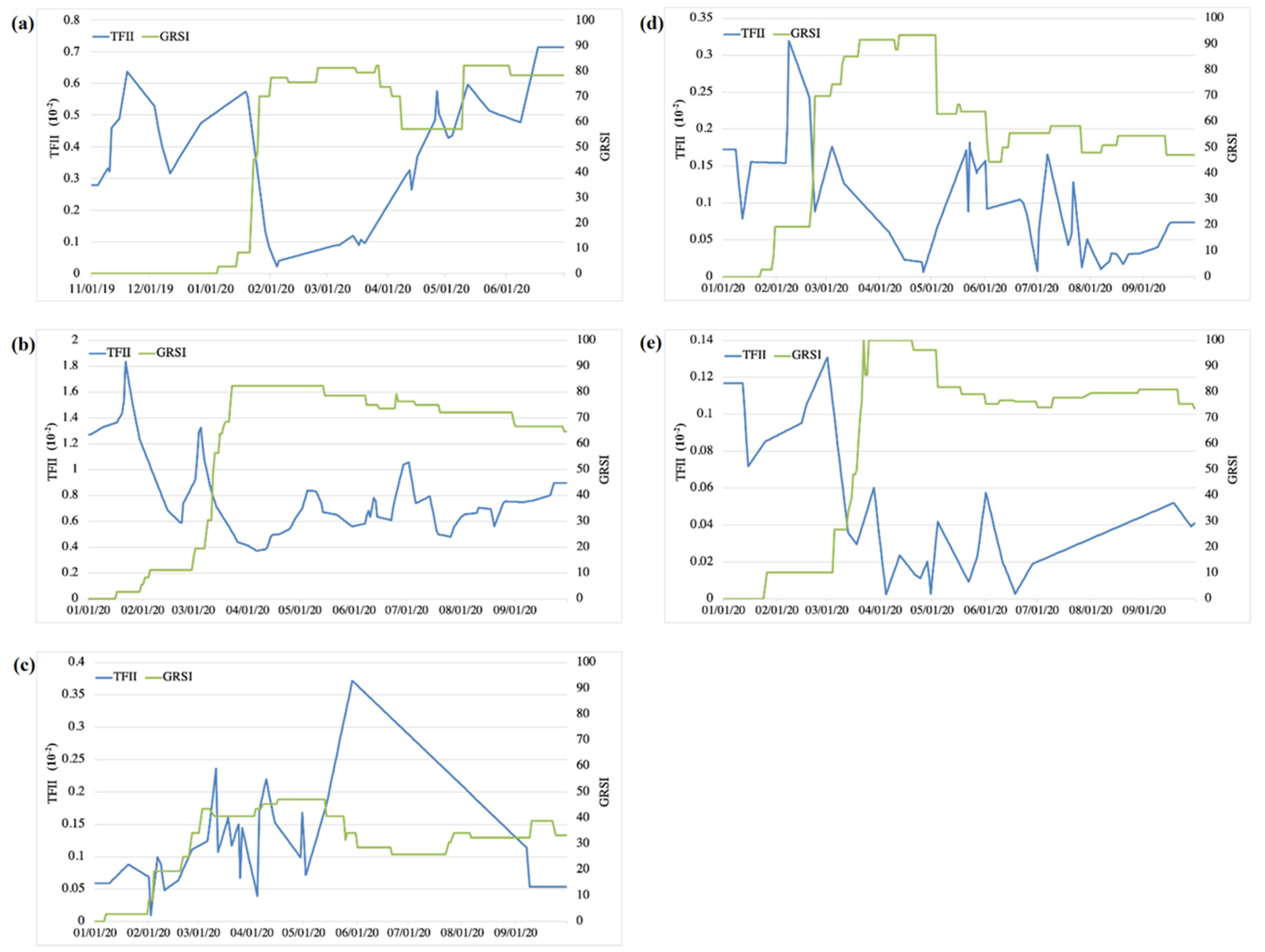
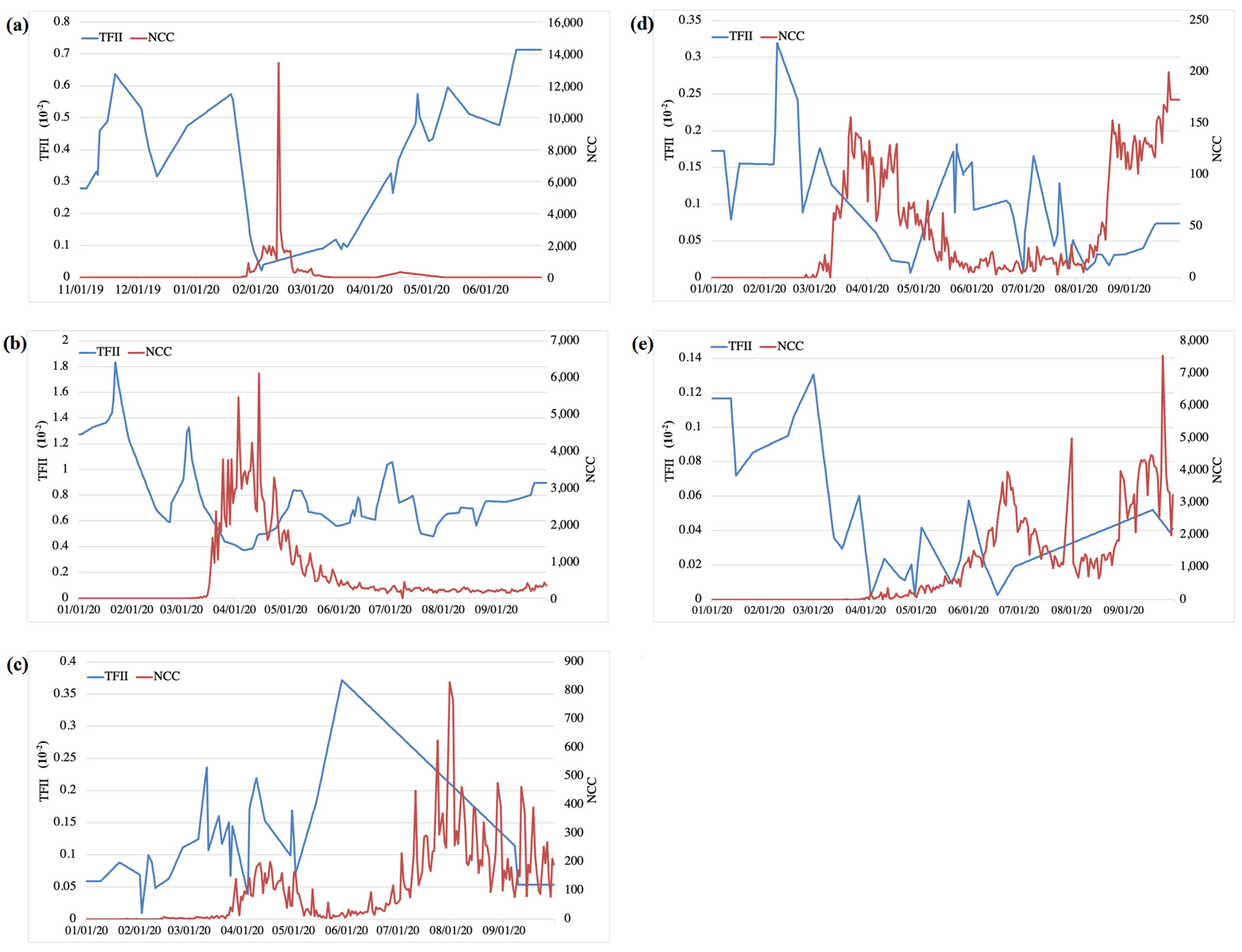
  • We compare our trend data with COVID-19 data and government response index provided by the Oxford COVID-19 Government Response Tracker [18], we validated the potential of using traffic density through our methods as an effective tool to analyze the impact of extreme events (COVID-19 in this case) at a small geographic scale, to benefit more timely decision support at the global level.
The remainder of this paper is as follows: Section 2 provides a detailed literature review on relevant works (both in vehicle detection and COVID-19 impact), while Section 3 provides details about the study areas and datasets used for this study. Section 4 presents our proposed vehicle detection methods on the study areas, and in Section 5 we analyze and evaluate the resulting traffic density results through trend analysis against the known data from the public. Finally, we conclude our findings in this paper by discussing the potential challenges of this work and outlook its potential future applications.

2. Related Works

We consider that our study is tied to two relevant topics: 1. Vehicle detection algorithms from remote-sensing satellite images; 2. Existing efforts on the use of mobility data for COVID-19 impact analysis. Therefore, in the following sections, we review both of these two topics.

2.1. Vehicle Detection Using High-Resolution Remote-Sensing Images

Detecting vehicles from remote-sensing images were mostly investigated in high-resolution data, with a ground sampling distance (GSD) of 1 m or less. Both traditional and deep-learning-based methods [19] were shown to be particularly effective in many relevant applications on vehicle counting [20,21]. Eslami and Faez presented a framework to detect vehicles and the road from high-resolution (0.6–1.0 m) panchromatic images in non-urban areas. They first used Hough transform and parallel lines detection to extract roads and then recognized traffic by using the artificial immune network concept [22]; Tuermer et al. used a machine-learning method to detected vehicles at dense urban areas from airborne platform at a spatial resolution of 13 cm [23]; Eikvil, Aurdal, and Koren provided an automatic approach consisting of a segmentation step followed by object classification to detect vehicles in high-resolution satellite images with 0.6 m resolution [24]. With the development of deep learning and artificial neural network [25], some deep-learning-based methods also being used in high-resolution remote sensing-based vehicle detection in recent years [26,27,28,29]. Although applications on high-resolution images were exercised well, when applied to low-resolution images (e.g., 3 m resolution Planet images), there are a couple of shortcomings: (1) both the traditional and deep-learning-based methods extract textural and high-level features from the cars, while cars in the 3 m Planet image take only a few pixels thus these features have relatively low descriptive powers; (2) the deep-learning-based methods require a large amount of annotated data, while such data do not exist (partly due to that these are not permanent objects) or difficult to annotate; (3) most of the aforementioned work, due to the lack of temporal resolution for the high-resolution data they focused on, are cross-sectional studies and little attention has been given to longitudinal mobility change dynamics over a long period.

2.2. Correlating Mobility with COVID-19

Understanding the dynamics of human mobility change at high spatial-temporal resolution is critical for assessing the impacts of policy interventions during the COVID-19 pandemic. To better understand how the governmental intervention affects residential mobility patterns after the COVID-19 outbreak, studies examine how social distancing intervention affects mobility patterns emerged recently and yielded mixed findings [30,31,32,33]. Badr et al. used an anonymized mobile phone data to analyze human mobility change during the COVID-19 period at the US county level, and the analyzed trends in human movement patterns were further compared with the temporal epidemiological dataset to evaluate how effective social distancing to mitigate COVID-19 transmission in the USA [33]; Gao et al. used county level aggregated anonymous mobile phone location data to calculate the daily travel distance and home dwell time thus assess how human mobility changes along with the trend of COVID-19 cases in the USA [31]. Kang et al. used anonymous mobile phone data to compute origin-to-destination (OD) flow at different geographical scales (census tract, county, and state) to reflect human mobility dynamics during the COVID-19 pandemic [30]. Pepe et al. used the anonymous smartphone data to calculate mobility metrics as a proxy of human mobility in order to better understand how national lockdown impacted Italy at a sub-national scale [32].
However, due to the mobile phone data not always being available in some areas, conducting a mobility analysis remains difficult especially for underdeveloped countries; less attention has been given to using vehicle detection methods to explore the mobility pattern changes during the COVID-19 pandemic, and we propose a novel vehicle detection method combining radiometric correction, road mask generation, and morphological-based vehicle-detection algorithm to calculate the traffic volume from the high-resolution satellite images. We apply this approach to multiple cities around the world and further examine how social distancing interventions affect human mobility during the COVID-19 period at a precise geographical scale. Our model can support more timely policy making around social distancing at a small geography scale and inform future public health decision making to fight against the COVID-19 pandemic.

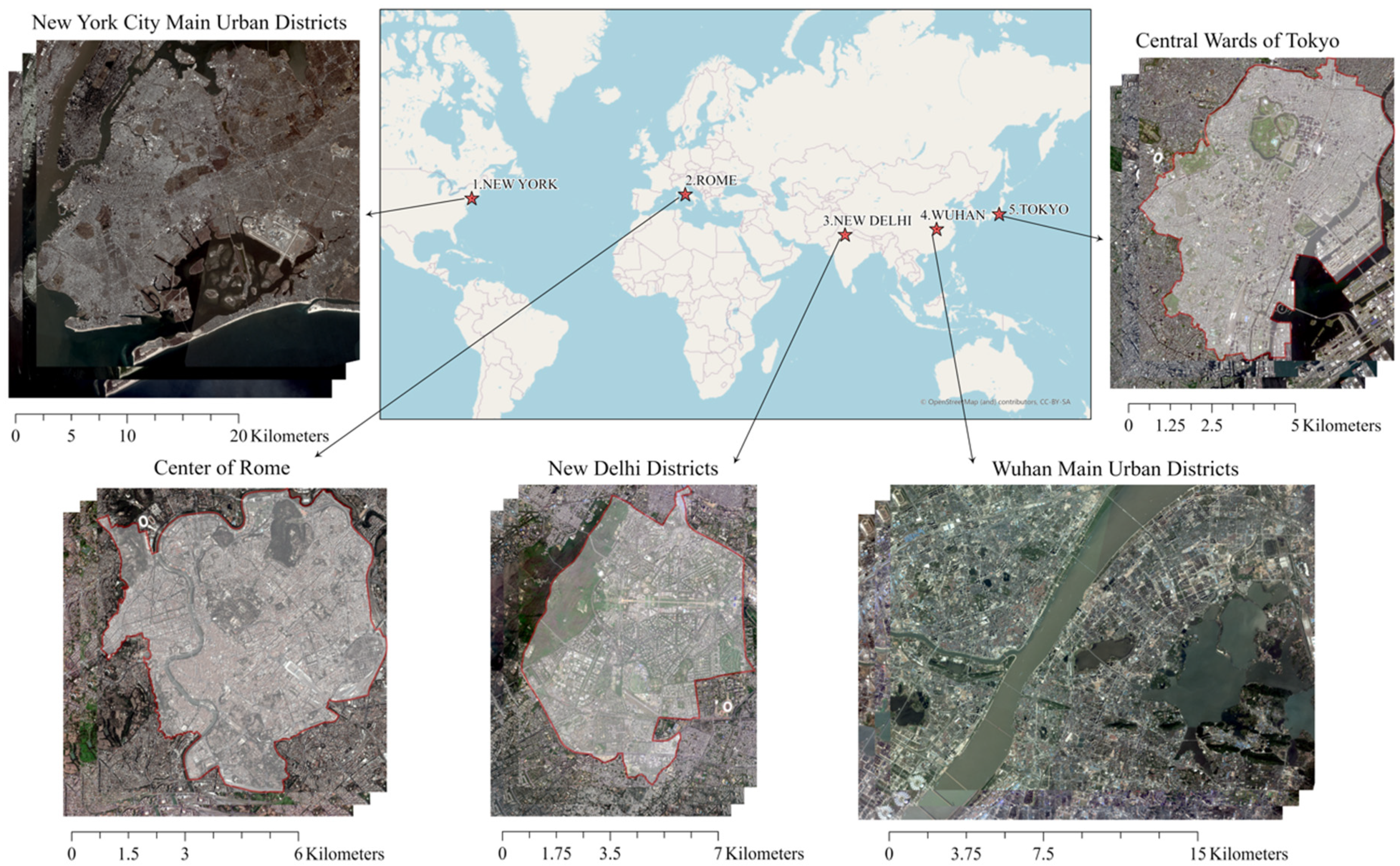
3. Study Areas and Data

Study areas: after the initial outbreak in Wuhan, China at the end of 2019 [34], the COVID-19 virus swiftly spread all over the world, the epic center shifted to east Asia (i.e., Japan) in early February and moved to the Middle East and Europe (i.e., Italy) in mid-February [35], and after March, the confirmed cases sharply increased in the United States and India making them the world centers of crisis [36,37]. Our study areas cover five representative cities (or districts in cities) in diverse geographical locations (see Figure 1) that have been reported to be impacted by the coronavirus and evaluated as epicenters [35], including: (1) Wuhan main urban districts (Jiang’an, Qiaokou, Hanyang, Jianghan, Wuchang, Qingshan, and Hongshan), China; (2) central wards of Tokyo (Chiyoda, Chūō, and Minato), Japan; (3) center of Rome (Municipio I and Municipio II), Italy; (4) New Delhi (New Delhi Municipal council area), India; (5) New York City main urban districts (Brooklyn, Queens, and Manhattan), USA.
Planet image data: We downloaded the PlanetScope 3B level images for these study areas, the images are 4-band (Red, Green, Blue, and Near-infrared (NIR)) multispectral images at a 3 m spatial resolution, with a 12-bit radiometric depth, TOA (top-of-atmosphere) corrected. The misalignment between different images is ignorable, since Planet uses a geo-registration process to enrich the geolocation consistencies among the images (0.7–5 pixels) [38], and the off-nadir angle is small (within 20°) with minimal relief differences [16]. Planet data processing systems perform a tie point-based data correction in their pipeline, meaning that these are pre-registered. In our experiments, we observe such errors can be ignored because the data we used have a registration error of less than 1 pixel, therefore we did not include a registration procedure; in general the registration can be performed using tie points through affine or projective transformations. We took the data from November 2019 to September 2020 (as of the date of the experiments). Since we noted that the COVID-19 confirmed cases did not change in Wuhan from June 2020 and the relevant policy to enforce social distancing (e.g., lockdown) ended earlier, the dates selected for Wuhan were from November 2019 to June 2020 with the intention to capture the possible impact. Dates of data for other regions listed above are from January 2020 to September 2020. We pre-filtered data based on the cloud level and the radiometric quality of the data (e.g., blurriness), and a summary of statistics of the selected images is in Table 1.
Road networks: Given the challenge of vehicle detection of the 3 m resolution data, we take the road network data from OSM as auxiliary data for our approach. OSM is a publicly available, volunteer-contributed repository of geographic information [17] and the completeness of the road networks in OSM has reached 83% [39]. In spite of the OSM dataset being created based on volunteer efforts, a study shows OSM has a high positional accuracy of 95% [40] and the positional accuracy is normally higher in areas with population-dense urban regions [41].
Additional data for validation analysis: we collect available public COVID-19 data in our study areas for validation, which include: (1) the COVID-19 data provided by the National Science Foundation Spatiotemporal Innovation Center [42]. The data are organized by both daily report and time-series summary for state/province level including confirmed, tested, death, recovered case numbers; and (2) the Government Response Stringency Index (GRSI) used in the Oxford COVID-19 Government Response Tracker [18]. The index quantifies the response policies into numbers and then takes the average. The policies include school and business closure, public event cancelation, etc. We use the GRSI as a proxy for governments’ responsiveness towards the COVID-19 crisis [35].

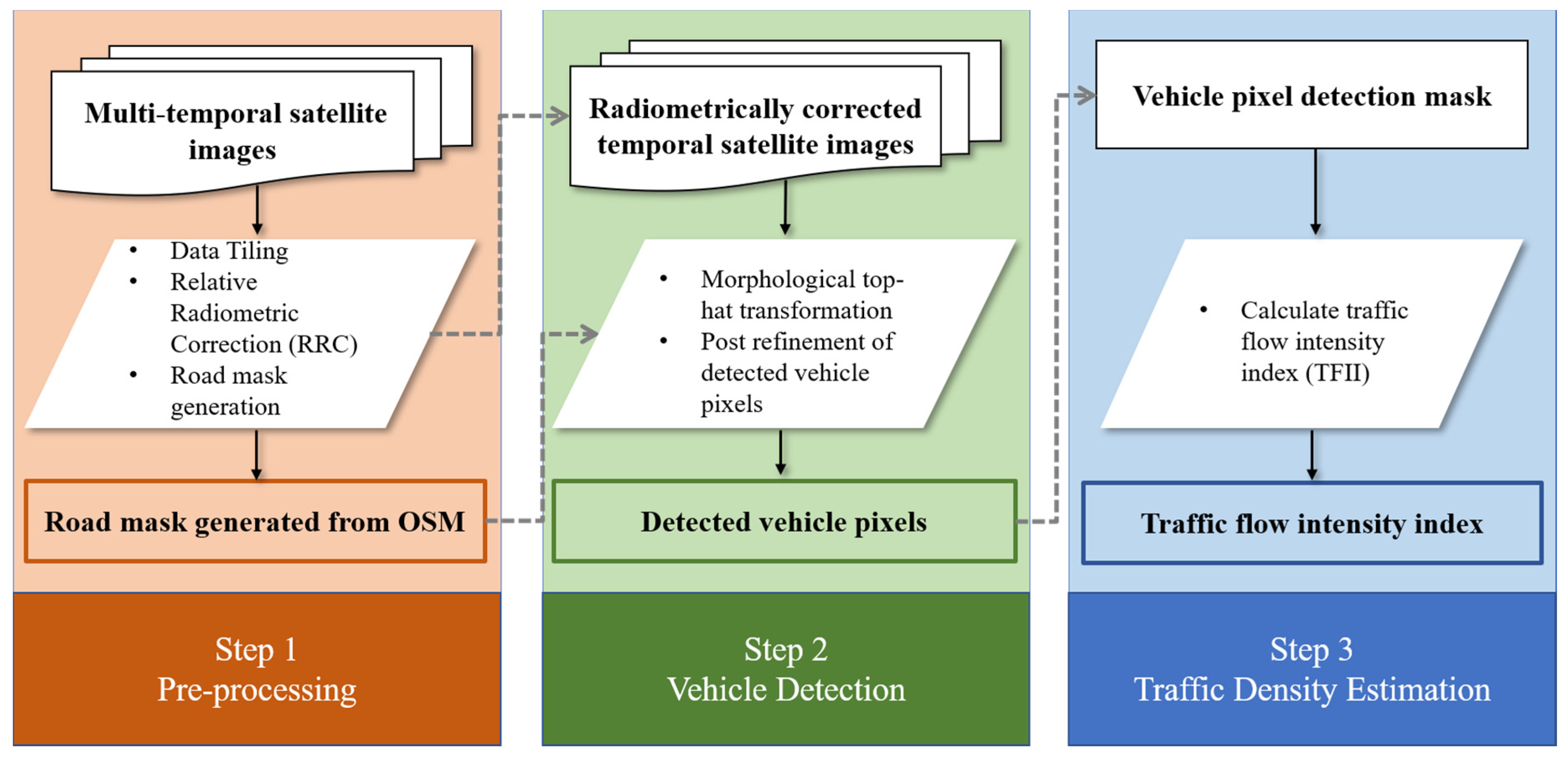
4. The Proposed Vehicle Detection and Traffic Density Estimation Framework

Our proposed vehicle-detection method is based on a background subtraction method [43], by first generating a background image from the multi-temporal images, and then subtracting the background images to identify moving objects. Such a process requires consistent radiometry along with the multi-temporal images which, however, due to the varying sun angle, atmospheric effects and sensor configurations, is hard to match with the raw images [44]. In addition, once the vehicle pixels have been detected, traffic density needs to be computed as a normalized parameter to perform our trend analysis. Therefore, our method consists of three steps: first, radiometrically corrected images and road mask need to be prepared for detection framework; second, a morphological-based vehicle detection method is conducted to capture vehicle pixels; third, traffic flow intensity index is calculated to capture traffic density for each temporal scene. The general workflow diagram of this article is depicted in Figure 2.

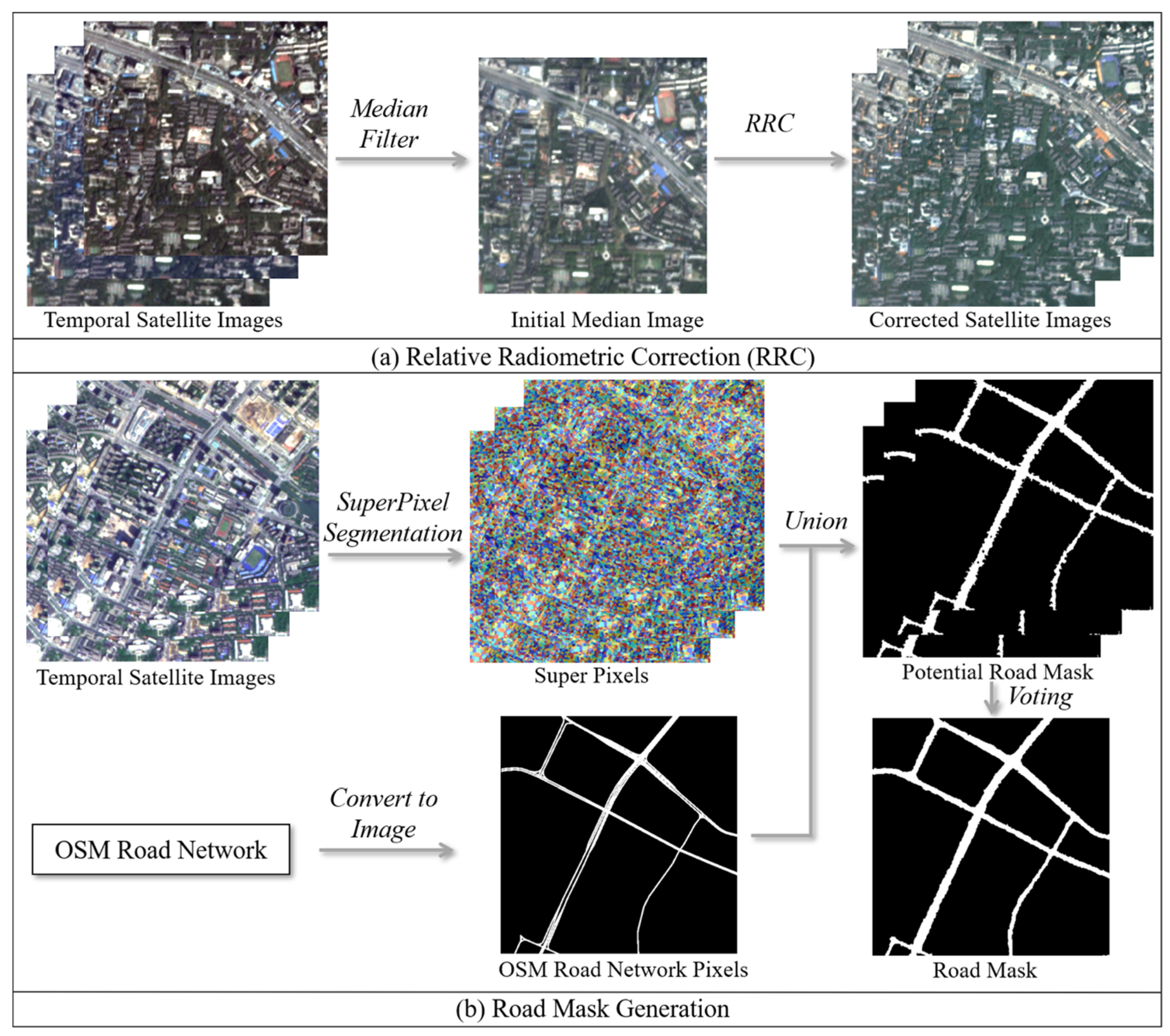
4.1. Pre-Processing—Radiometric Correction and Road Mask Refinement

Satellite images vary in their spectral appearances due to factors such as sunlight angle, existence of cloud, shadows, etc., thus, we apply relative radiometric correction (RRC) on the temporal images from the Planet satellite to yield radiometrically coherent images for performing temporal analysis on homogenous images. The RRC methods often require a reference image, to which the radiances of other images are aligned. Given the high temporal resolution of images, we take the median of them as the reference image representing the most frequent intensity value at each pixel location throughout the time. Specifically, we consider that the road pixels represent concrete or asphalt and appearance to temporally invariant, and we therefore take the large number of road pixels masked by the OSM road network data, to compute the ratio of correction. Our adapted RRC algorithm rescales each image using two types of scaling factors between reference and target images. If the pixel values are brighter than the mean value of road pixels in the reference image, we calculate brighter scaling factor B i by using the median ratio of positive differences. If the pixel values are darker, we obtain darker scaling factor D i , vice versa. The radiometrically corrected images are then computed by scaling factors correction for each pixel difference and then added to the mean value of the reference image (see Figure 3a).
B i   =   M e d i a n [ ( P r e f , m , n     M ) / ( P i , m , n     M ) ] ,           f o r   ( P i , m , n     M ) > 0 ,   ( P r e f , m , n     M )   > 0
D i = M e d i a n [ ( P r e f , m , n M ) / ( P i , m , n M ) ] , f o r   ( P i , m , n     M ) < 0 ,   ( P r e f , m , n     M )   < 0
where P i , m , n refers pixel values for row m, column n in ith image, P r e f , m , n refers pixel values for row m, column n in reference image, M is the mean value of road pixels in a reference image.
To improve the robustness of the vehicle detection, we take advantage of the OSM road network vector data to constrain the detection. Note that such road network data can be also obtained through directly predicting the road pixels via deep learning-based methods [45] in case that OSM data is not available. The OSM road network vector data come with inaccurate road width and have minor misalignment [41] to the images, and therefore we propose a simple refinement procedure to adapt the road network data to the multi-temporal images (Figure 3b): we perform a super-pixel segmentation [46] method on each of the multi-temporal images and use the following formula to generate a road mask for each of the images:
r o a d m a s k _ j   = i S j i
where S j i refers to super pixels of image j in which the OSM road network pixels (formatted/converted from the OSM road vector data) present, and the road mask for image j takes the union of all these super pixels to capture the actual shape of the road. The final road mask takes the pixel-level majority vote over all the r o a d m a s k _ j   to improve the OSM road networks for our subsequent steps for vehicle detection.

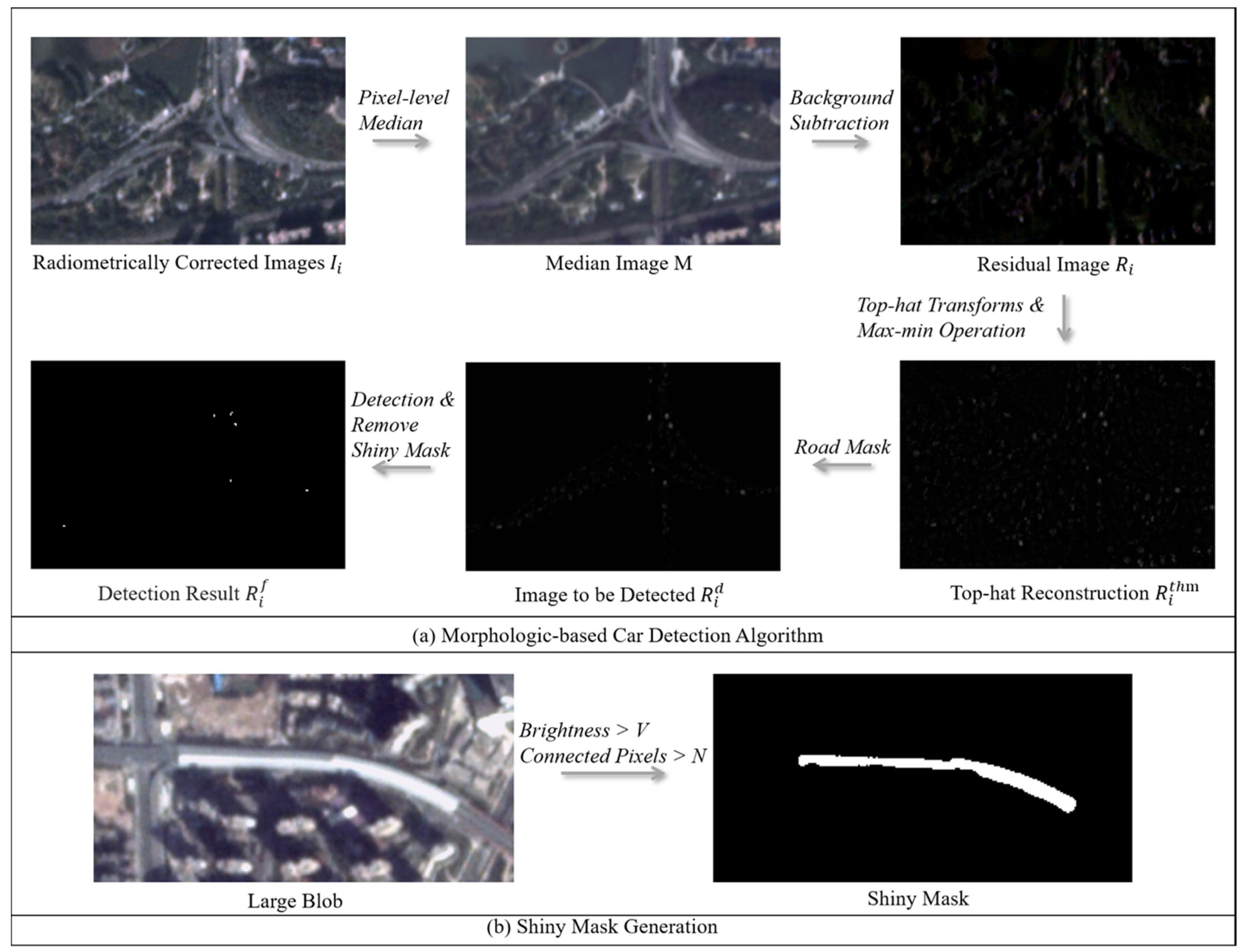
4.2. The Proposed Morphology-Based Vehicle Detection Method

As discussed in Section 1, the existing high-performance vehicle detection algorithms, both traditional and deep-learning-based, when applied to the relatively low-resolution Planet images (3-m), face two challenges: (1) the number of pixels a car takes is in the level of tens, thus they can hardly utilize complex and descriptive features (either manually crafted or learned) for detection; (2) training data of these moving vehicle can be difficult to label in such low-resolution data images. Therefore, we propose to utilize simple appearance features, with the aid of the road masks as described in Section 4.1., to detect car candidates. We note that in such a low-resolution image, the vehicles on the road (concrete or asphalt) appear to be with high contrast and blob-like shapes, therefore, we devise our approach to capture such features by utilizing a morphology top-hat transformation [47,48,49] as this has been shown to be effective to capture such features.
Our proposed approach is described as follows (Figure 4): since cars on the road can be either brighter or darker than the road pixels, as a first step, we take a background subtraction approach, to subtract a median image M, calculated by taking the pixel-level median over all the multitemporal images, from each of the image I i , resulting in a residual image R i . The median image is regarded as the background image representing the static objects in the scene, thus the residual image R i present mostly the moving objects, and when masked by the road mask (described in Section 4.1.), its brightness mostly reflects potential car pixels or other objects on the road that were mainly caused by either construction or illumination changes. In a second step, we apply a multi-directional morphological top-hat transformation on each of the residual images R i , as used in Drouyer and de Franchis’ method [50], which uses linear structuring elements with four directions (0°, 45°, 90°, and 135°, with a radius of 7 pixels) separately on R i to capture the feature in an isotropic manner and takes the pixel level minimum resulting the top-hat transformed image R i t h . The same process is applied to each band of the multispectral images, and a pixel-level maximum is taken to form the final morphology-based top-hat reconstruction R i t h m , which in summary is a max-min operation:
R i t h m = max j b a n d s min d d i r { T H ( R i j , S e d ) }
where R i j is refers to the jth band of the ith residual image R i , and TH(•) refers to the top-hat reconstruction [49] and S e d refers to the linear structuring element in the direction of d.
The top-hat reconstruction R i t h m   as described above can effectively extract blob-shaped regions on the roads. However, we note in some cases the concrete road, due to the specular reflection, appears to be extremely bright on some of the images in the multitemporal images that saturate any detectable contrast, resulting in large blobs, which can be deleted by connected component analysis [51]. Therefore, in the third step, we further apply simple masking by generating a so-called “shiny mask” (see Figure 4b), through thresholding the original image I i (after radiometric correction). The threshold is set conservatively to avoid potential deletion of the correct vehicle detections. Brightness threshold V and connected component size N are set to create “shiny mask” (we use 0.78 out of 1 and 500 pixel size in the experiments).
In the final step, a road mask is used to validate any car pixels inside road region to get R i d . A dynamic thresholding process is applied to detect car pixels. We start to compute maximum value Tmax from R i d and set threshold as Tmax. At each time, potential pixels will be extracted and selected by at least L = 2 connected pixels, Tmax will be re-calculated by the multiple of a scale index R = 0.9, until Tmax is smaller than a threshold X = 0.13 out of 1. The “shiny mask” is simply applied to this binary image to invalidate any car pixels inside that region. Finally, we obtain R i f to represent our final car pixels for each of the image. It is worth noting that most of the parameters are cut thresholds for linear index, therefore they can be intuitively tunable. We decide to set the parameter empirically by understanding appropriately the values of the detectors, instead of learning from a specific dataset, thus the parameters are not necessarily optimal to a particular dataset but explainable and potentially more generalizable.

4.3. Traffic Flow Intensity Index (TFII)

To reach a consistent measurement of traffic density across different image i with special consideration focus on the spatial heterogeneity of the road network coverages, we calculate our traffic flow intensity index T as:
T i = N ( v , i )   N ( r , i ) · s
where N ( v , i )   denotes the total number of detected vehicle pixels in image i , and N ( r , i ) is the total number of road mask pixels within image i . This serves as a normalization indicating how busy the roads (in this case, the proportion of road that was occupied by vehicles) are given a specific day. Given the large number of road pixels, the resulting index can be numerically small. Therefore, normalize the traffic flow intensity index (TFII) with a constant factor of s = 100 for numerical purpose.

5. Experimental Results and Analysis

In this section, we first validate our vehicle detection algorithm and its detection accuracy using seven representative regions to understand the performance of the car detection, and then we scale this method by applying it to the study areas mentioned in Section 3, and finally analyze the results.

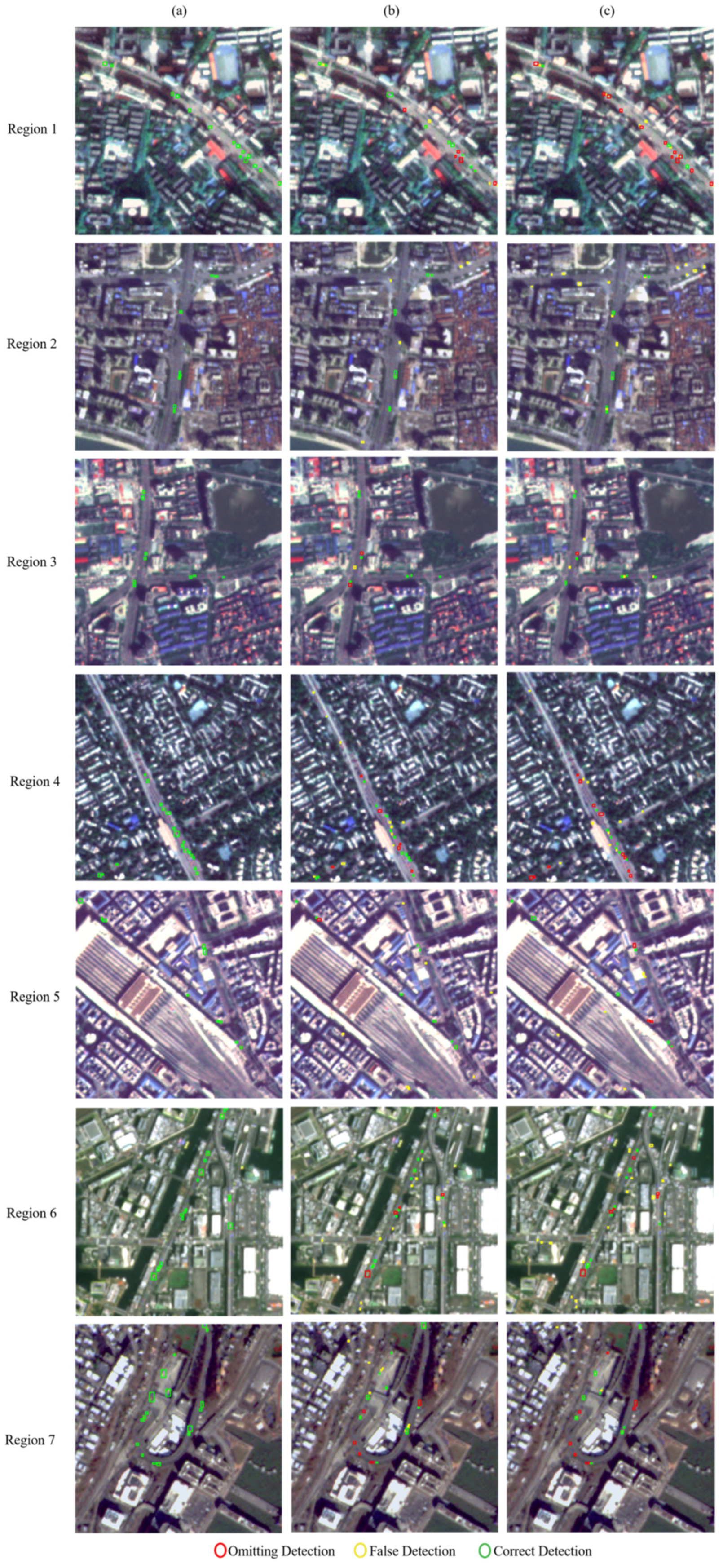
5.1. Validation of Vehicle Detection Algorithm

To assess the accuracy and robustness of our proposed vehicle detection algorithm quantitatively, we select seven representative test regions across all study cities that cover different urban and road conditions (i.e., roads across commercial district, roads across residential area, transportation junction, road intersection, bridge, overpass, etc.). We manually labeled the vehicle objects and then calculated the precision, recall and F1 score [52] for our detection results, the total number of labeled objects is 149. The area of each site covers a region of 1.2 × 1.2 km2, due to the vehicle object being too small to be recognized at the full 1.2 × 1.2 km2 mapping scale, and we provide the enlarged view for part of each test region to demonstrate the detection result, shown as Figure 5. Considering that the proposed algorithm assumes blob shapes on the roads as vehicles, it inherently tends to produce false positives, therefore image scenes with sparse vehicles can be particularly useful to test the performance of the algorithms. Given the low resolution of the image, we used a relatively relaxed strategy in counting correct detections: we consider a prediction as “correct”, if there are overlaps between the predicted rectangle and the ground-truth rectangle. An example is shown in Figure 5, in which the green rectangles indicate the correct detection, the red rectangles refer to omissions and yellow rectangles refer to false detections. We have also compared our method with Drouyer and de Franchis’ method [50]. It shows that our detection method produces more correct detections. Statistics of our method and the comparing method applied to the seven test regions are shown in Table 2, and it can be seen that our method on these test regions has achieved an overall approximately 68% on average in terms of F1 score, which is 14% higher than that of the comparison method. To dive into the vehicle detection accuracy result in each region, our method outperformed the comparison method in almost all regions, it is worth noting that our result accuracy in region 1 is significantly better, this benefits from the relative radiometric correction procedure of our method, since the raw image data have a relatively higher value of blue band than red and green band. This accuracy test provides us a rough estimation on the fidelity of the generated data when applying to bigger regions of different cities.

5.2. Analyze Traffic Flow Dynamics

We applied our proposed method to the five cities/districts mentioned in Section 3. We computed the TFII to indicate the traffic-flow density for each city/district. Given the areas of each city is different, each city/district is evaluated using the varying number of tiles. Since images of different tiles may have different availability, we resample these points through a bilinear interpolation and take the average. To analyze the significance of our proposed method, we further use the Pearson correlation coefficient [53] to evaluate the predicted TFII with the known public data mentioned in Section 3, which includes (1) the GRSI [18], and (2) the newly confirmed COVID-19 cases (NCC) at each city [42]. The trend plots are shown in Figure 6 and Figure 7, the Pearson correlation coefficient and statistical significant [54] are shown as Table 3. We expect that our predicted TFII, if successful, should indicate at least qualitatively significances in terms of (negative) correlations with the GRSI, since the GRSI directly relates to government responses in practicing social distancing (e.g., lockdown, etc.), which may lead to fewer vehicles on roads. This may potentially be related to the newly confirmed cases as well, since this creates a social/soft constraint that implicitly presents risks of mobility, thus leading to reduced road vehicles as well.
With an analysis of Figure 6 and Figure 7, we can observe that in general the trend of traffic density is negatively correlated with the GRSI, and such a trend is reflected specifically well for the city of Rome, New York and New Delhi, with a Pearson correlation coefficient of −0.48, −0.75 and −0.87, with moderate correlation with Wuhan (−0.33), and low correlation with the Tokyo data (0.18). While the correlation with the newly confirmed cases is still showing as negative but less strong than GRSI, shown in Table 3. In the following paragraphs we analyze each city in detail.
Wuhan: The experimental region of Wuhan covers in total an area of 305.67 km2, including the core urban districts, Wuchang, Hankou, and Hanyang. It was noted that since Wuhan was likely the first city that reported the outbreak of COVID-19, it is subject to strict control of social distancing, therefore, the lockdown and stay-at-home requirement were exercised at the city level, starting in early February till the beginning of April 2020. This is well reflected in the GRSI. There was continuous government intervention after April as indicated by the GRSI, while apparently not at a level of lockdown on the roads, as our curve indicates the active TFII afterwards. In the meantime, we observe that the TFII is negatively correlated with the NCC, with a Pearson correlation coefficient of −0.33, as the only wave appears to be around February 2020, the TFII declines to the lowest point, and after that the cases are well under control, thus the NCC does not pose much soft constraints to the traffic or human mobility.
New York: Our experimental region of New York covers the main urban districts (Brooklyn, Queens, and Manhattan), totaling an area of 849.70 km2. To accommodate the dimension of single Planet images, the area is subdivided by nine tiles and the curve within different tiles has minor variations and the average of them is shown in Figure 6b and Figure 7b. The GRSI and the NCC show that the surge of confirmed cases started in early March and reached the summit in April. We observed a high correlation (Pearson correlation coefficient: −0.75) with the GRSI, that the TFII is significantly low starting from March, and we note the NCC starts to get flatten in late May while GRSI remains to be high, therefore we can observe that the TFII is relatively low and only have a minor increase towards September 2020. We also observed the TFII is negatively correlated with NCC, with a Pearson correlation coefficient of −0.51, which shows when the confirmed cases surging, the streets are emptier due to the practice of governmental interventions and reduced transportation needs. We have further plotted these nine tiles in Figure 8, and it shows that the western part of New York City (Brooklyn and Manhattan) has a significant drop of TFII when the pandemic wage on and intervention involved in and the TFII for the rest part of the city (Queens) had a less degree of drop. We also see as the pandemic alleviated after May, and the traffic recovered faster in the eastern part of the New York City.
Tokyo: Our experimental region for Tokyo is relatively small, covering three districts, including Chiyoda, Chūō, and Minato, which totals an area of 69 km2. The GRSI and NCC in this area show that Tokyo’s COVID-19 cases started to increase around mid of March, while the government intervention had already performed at least one month ahead. Even though the overall strength of intervention (indicated by GRSI) in Tokyo is significantly weaker than the remaining four cities, our TFII has indicated that mobility was consistently low since February 2020. Starting from May, the GRSI shows less government intervention which opens the traffic, in the meantime, TFII in Tokyo increased significantly and reached the peak around July until the second COVID-19 outbreak in July, from when the traffic flow steadily decreased due to voluntary social distancing, as the government intervention played the same role as before. It worth noting that the correlation between TFII and GRSI or NCC calculated for Tokyo is less significant compare with the other four cities. The GRSI not significantly capturing lockdown and opening was likely the cause of the low correlation between the GRSI and TFII. Tokyo as the largest mega-region in the world has experienced rapid development of public transit and it has a complex public transit system that contains different traffic modes to mitigate the high population density challenge and the huge amount of traffic pressure [55]. The less significant correlation between TFII and NCC may be caused by the TFII only captured people travel by car, which is just a proportion of the total daily commuting population since people are also traveling by metro and trains in Tokyo.
Rome: The experimental region of Rome covers an area of 60 km2 (city center). The city experienced two waves of COVID-19 cases increasing, one in April and another in August. Our results show the TFII is negatively correlated with both GRSI and NCC, with a Pearson correlation indexes as −0.48 and −0.50, respectively. The government initiated strong intervention (high GRSI) around April and the computed TFII indicates that the traffic volume has decreased significantly. The GRSI shows that the government intervention slightly loosed starting from May, and the TFII shows a general trend of increased traffic density until August with few local peaks and valleys that could be due to the time-of-the-day difference of collected images. Since the second wave hit Rome in August, the TFII remained at a low level after that.
New Delhi: Our experimental region in New Delhi covers an area of 75 km2. It is shown in Figure 6e and Figure 7e that although the number of newly confirmed cases starts to increase in May, the GRSI shows that the government intervention plays a role in mid-March and keeps high as of September 2020. Our extracted TFII indicated that the traffic density has significantly reduced in Mid-March, showing a very high correlation with the GRSI (Pearson correlation coefficient: −0.88). The result also shows traffic density negatively correlated with the growing number of cases, with a Pearson correlation coefficient of −0.34.

5.3. Discussion

Our experiments over the five cities/districts show when the COVID-19 disease outbreak and local policy intervention are combined, the predicted traffic density significantly declines which indicates the local residents are positively exercising social distancing. Among the five cities/districts, four of them have shown notable negative correlation (0.33 and above) between the predicted traffic flow intensity index and the government interventions, with only the Tokyo area being less correlated, which is potentially due to the sparsity of the images and outliers in one specific day. In addition, although the predicted TFII trends show a certain level of variations (as shown in Figure 6, Figure 7 and Figure 8), it generally captures the fact of the reduced traffic volume, as validated both in the five-city study and our accuracy test (68% F1 score). It is worth mentioning that the temporal pattern of traffic volumes such as seasonal trend (month-of-the-year) or commuter pattern (day-of-the-week or rush hrs. vs. non-rush hrs.) may also play a role in trend analysis and affect the correlation result [56]. However, to obtain more accurate measures, we would need thousands of images to select images that take at exactly the same time of the day throughout a period, at the moment, existing constellations do not offer this capacity yet. Due to the limited flexibility of image acquisition times, the current study only looks for the general trend in a relatively long time period. The TFII also shows a reasonable correlation (negatively, mostly above 0.3) with the NCC, showing that not only the government intervention plays a role, but also the NCC serves as a soft constrain that drives the reduced traffic/mobile activities.

6. Conclusions

In this paper, we utilized the multitemporal Planet satellite image data to develop a vehicle detection method in order to examine the mobility changes in different cities around the world in response to the COVID-19 pandemic. Planet satellite images have a 3 m spatial resolution; thus, vehicle detection presents as an extremely challenging task with very few pre-existing methods applicable. We improved from the previous method [50] by incorporating a series of new components including radiometric correction, road shape adjustment, shiny mask generation and road mask generation for result fusion. We demonstrate from our experiment that our proposed vehicle detection algorithm has achieved an F1 score of 68% in our test areas, which outperforms a recent method [50] used for Planet images. We further scale our proposed method to detect high-temporal dynamics of vehicles in five cities/districts (total over ~1360 km2, with an average of 42 temporal images covering these regions). Our correlation analysis with the GRSI and the NCC, strongly supports the observations that the detected vehicle and the yielded traffic flow intensity index (TFII) merely using single-source satellite images present a strong and objective measure of the actual traffic/mobile patterns during the COVID-19 period. The high (Pearson) correlation coefficients between our TFII and the GRSI and NCC, further support our hypothesis that this 3 m resolution high-temporal remote-sensing data can provide valid information at the city or district level to assess the mobility patterns during the COVID-19. Such a capability can be further applied to consistently monitor non-natural disasters and evaluate the potential impact of extreme events globally. During our experiments, we have also found several drawbacks of our approach: first, our paper offers some instrumental insights that low-resolution satellite images can be utilized to estimate traffic intensity at a small geographical scale, it is worth noting that there are other sources of information like mobile phone data or traffic counter data that are also able to estimate traffic intensity, a comparative analysis of how satellite-based and other approach should be conducted in the future to assess how they perform differently; second, the relatively low resolution may produce outliers in vehicle detection, especially on occasions of high variation of illumination changes, since our approach is based on a simple appearance feature based on morphological transformations, we are aware that in such a low-resolution data, it is impossible to obtain highly accurate results for individual car detection, our final products are the traffic flow density rather than individual cars to provide a relatively coarse traffic measure in order to understand extreme events; third, although for each of our test regions, we have collected weekly or bi-weekly image on average, often some of these images might be discarded due to the high cloud coverage and illuminations, thus with an even higher temporal resolution, the prediction may yield redundancies to offer more trustworthy results. In our future work, we aim to attempt to improve our method by incorporating more semantic information predicted from the image to generate better traffic predictions and apply our method at the country level.

Author Contributions

Conceptualization, R.Q. and Y.C.; methodology, Y.C. and R.Q.; coding, Y.C., G.Z., and R.Q.; data processing, Y.C., G.Z., H.A.; analysis, Y.C. and R.Q.; writing—initial draft, Y.C., G.Z. and H.A.; writing—refined draft, Y.C. and R.Q.; supervision, R.Q.; review and editing, R.Q.; All authors have read and agreed to the published version of the manuscript.

Funding

R.Q. is partially funded by Office of Naval Research (Award No. N000141712928 and N00014-20-1-2141).

Institutional Review Board Statement

Not applicable.

Informed Consent Statement

Not applicable.

Data Availability Statement

Not applicable.

Acknowledgments

The authors would like to acknowledge Planet Inc. for providing the Planet images through their research and education program.

Conflicts of Interest

The authors declare no conflict of interest.

References

  1. Rothan, H.A.; Byrareddy, S.N. The epidemiology and pathogenesis of coronavirus disease (COVID-19) outbreak. J. Autoimmun. 2020, 109, 102433. [Google Scholar] [CrossRef] [PubMed]
  2. Spinelli, A.; Pellino, G. COVID-19 pandemic: Perspectives on an unfolding crisis. Br. J. Surg. 2020, 107, 785–787. [Google Scholar] [CrossRef] [PubMed] [Green Version]
  3. Haushofer, J.; Metcalf, C.J.E. Which interventions work best in a pandemic? Science 2020, 368, 1063–1065. [Google Scholar] [CrossRef] [PubMed]
  4. Dong, E.; Du, H.; Gardner, L. An interactive web-based dashboard to track COVID-19 in real time. Lancet Infect. Dis. 2020, 20, 533–534. [Google Scholar] [CrossRef]
  5. Askitas, N.; Tatsiramos, K.; Verheyden, B. Lockdown Strategies, Mobility Patterns and Covid-19. arXiv 2020, arXiv:2006.00531. [Google Scholar]
  6. Alexander, D.; Karger, E. Do Stay-at-Home Orders Cause People to Stay at Home? Effects of Stay-at-Home Orders on Consumer Behavior. SSRN Electron. J. 2020. [Google Scholar] [CrossRef]
  7. Tull, M.T.; Edmonds, K.A.; Scamaldo, K.M.; Richmond, J.R.; Rose, J.P.; Gratz, K.L. Psychological Outcomes Associated with Stay-at-Home Orders and the Perceived Impact of COVID-19 on Daily Life. Psychiatry Res. 2020, 289, 113098. [Google Scholar] [CrossRef]
  8. Chinazzi, M.; Davis, J.T.; Ajelli, M.; Gioannini, C.; Litvinova, M.; Merler, S.; Piontti, A.P.Y.; Mu, K.; Rossi, L.; Sun, K.; et al. The effect of travel restrictions on the spread of the 2019 novel coronavirus (COVID-19) outbreak. Science 2020, 368, 395–400. [Google Scholar] [CrossRef] [Green Version]
  9. Gualtieri, G.; Brilli, L.; Carotenuto, F.; Vagnoli, C.; Zaldei, A.; Gioli, B. Quantifying road traffic impact on air quality in urban areas: A Covid19-induced lockdown analysis in Italy. Environ. Pollut. 2020, 267, 115682. [Google Scholar] [CrossRef]
  10. Warren, M.S.; Skillman, S.W. Mobility Changes in Response to COVID-19. arXiv 2020, arXiv:2003.14228. [Google Scholar]
  11. Bisanzio, D.; Kraemer, M.U.; Bogoch, I.; Brewer, T.; Brownstein, J.S.; Reithinger, R. Use of Twitter social media activity as a proxy for human mobility to predict the spatiotemporal spread of COVID-19 at global scale. Geospat. Health 2020, 15. [Google Scholar] [CrossRef] [PubMed]
  12. Lv, Z.; Pomeroy, J.W. Detecting intercepted snow on mountain needleleaf forest canopies using satellite remote sensing. Remote. Sens. Environ. 2019, 231, 111222. [Google Scholar] [CrossRef]
  13. Zurqani, H.A.; Post, C.J.; Mikhailova, E.A.; Allen, J.S. Mapping Urbanization Trends in a Forested Landscape Using Google Earth Engine. Remote. Sens. Earth Syst. Sci. 2019, 2, 173–182. [Google Scholar] [CrossRef]
  14. Orimoloye, I.; Mazinyo, S.P.; Kalumba, A.M.; Nel, W.; Adigun, A.I.; Ololade, O.O. Wetland shift monitoring using remote sensing and GIS techniques: Landscape dynamics and its implications on Isimangaliso Wetland Park, South Africa. Earth Sci. Inform. 2019, 12, 553–563. [Google Scholar] [CrossRef]
  15. Singh, S.; Reddy, C.S.; Pasha, S.V.; Dutta, K.; Saranya, K.R.L.; Satish, K.V. Modeling the spatial dynamics of deforestation and fragmentation using Multi-Layer Perceptron neural network and landscape fragmentation tool. Ecol. Eng. 2017, 99, 543–551. [Google Scholar] [CrossRef]
  16. Planet Team. Planet Application Program Interface: In Space for Life on Earth; Planet Team: San Francisco, CA, USA, 2017; Available online: https://api.planet.com (accessed on 6 January 2021).
  17. Haklay, M.; Weber, P. OpenStreetMap: User-Generated Street Maps. IEEE Pervasive Comput. 2008, 7, 12–18. [Google Scholar] [CrossRef] [Green Version]
  18. Hale, T.; Petherick, A.; Phillips, T.; Webster, S. Variation in Government Responses to COVID-19; Blavatnik School Working Paper; Blavatnik School of Government, University of Oxford: Oxford, UK, 2020; Volume 31. [Google Scholar]
  19. Goodfellow, I.; Bengio, Y.; Courville, A. Deep Learning; MIT Press Cambridge: Cambridge, MA, USA, 2016; Volume 1. [Google Scholar]
  20. Dai, Z.; Song, H.; Wang, X.; Fang, Y.; Yun, X.; Zhang, Z.; Li, H. Video-Based Vehicle Counting Framework. IEEE Access 2019, 7, 64460–64470. [Google Scholar] [CrossRef]
  21. Zhang, S.; Wu, G.; Costeira, J.P.; Moura, J.M.F. Fcn-rlstm: Deep Spatio-Temporal Neural Networks for Vehicle Counting in City Cameras. In Proceedings of the IEEE International Conference on Computer Vision, Venice, Italy, 22–29 October 2017; pp. 3667–3676. [Google Scholar]
  22. Eslami, M.; Faez, K. Automatic Traffic Monitoring from Satellite Images Using Artificial Immune System. In Lecture Notes in Computer Science; Springer Science and Business Media LLC: Berlin, Germany, 2010; pp. 170–179. [Google Scholar]
  23. Tuermer, S.; Kurz, F.; Reinartz, P.; Stilla, U. Airborne Vehicle Detection in Dense Urban Areas Using HoG Features and Disparity Maps. IEEE J. Sel. Top. Appl. Earth Obs. Remote. Sens. 2013, 6, 2327–2337. [Google Scholar] [CrossRef]
  24. Eikvil, L.; Aurdal, L.; Koren, H. Classification-based vehicle detection in high-resolution satellite images. ISPRS J. Photogramm. Remote. Sens. 2009, 64, 65–72. [Google Scholar] [CrossRef]
  25. Ma, L.; Liu, Y.; Zhang, X.; Ye, Y.; Yin, G.; Johnson, B.A. Deep learning in remote sensing applications: A meta-analysis and review. ISPRS J. Photogramm. Remote. Sens. 2019, 152, 166–177. [Google Scholar] [CrossRef]
  26. Jiang, Q.; Cao, L.; Cheng, M.; Wang, C.; Li, J. Deep Neural Networks-Based Vehicle Detection in Satellite Images. In Proceedings of the IEEE 2015 International Symposium on Bioelectronics and Bioinformatics (ISBB), Beijing, China, 14–17 October 2015; pp. 184–187. [Google Scholar]
  27. Liu, Y.; Liu, N.; Huo, H.; Fang, T. Vehicle Detection in High Resolution Satellite Images with Joint-Layer Deep Convolutional Neural Networks. In Proceedings of the 23rd International Conference on Mechatronics and Machine Vision in Practice (M2VIP), Nanjing, China, 28–30 November 2016; pp. 1–6. [Google Scholar]
  28. Chen, X.; Xiang, S.; Liu, C.-L.; Pan, C.-H. Vehicle Detection in Satellite Images by Hybrid Deep Convolutional Neural Networks. IEEE Geosci. Remote. Sens. Lett. 2014, 11, 1797–1801. [Google Scholar] [CrossRef]
  29. Sakai, K.; Seo, T.; Fuse, T. Traffic Density Estimation Method from Small Satellite Imagery: Towards Frequent Remote Sensing of Car Traffic. In Proceedings of the 2019 IEEE Intelligent Transportation Systems Conference (ITSC), Auckland, New Zealand, 27–30 October 2019; pp. 1776–1781. [Google Scholar]
  30. Kang, Y.; Gao, S.; Liang, Y.; Li, M.; Rao, J.; Kruse, J. Multiscale dynamic human mobility flow dataset in the U.S. during the COVID-19 epidemic. Sci. Data 2020, 7, 1–13. [Google Scholar] [CrossRef] [PubMed]
  31. Gao, S.; Rao, J.; Kang, Y.; Liang, Y.; Kruse, J.; Dopfer, D.; Sethi, A.K.; Reyes, J.F.M.; Yandell, B.S.; Patz, J.A. Association of Mobile Phone Location Data Indications of Travel and Stay-at-Home Mandates with COVID-19 Infection Rates in the US. JAMA Netw. Open 2020, 3, e2020485. [Google Scholar] [CrossRef] [PubMed]
  32. Pepe, E.; Bajardi, P.; Gauvin, L.; Privitera, F.; Lake, B.; Cattuto, C.; Tizzoni, M. COVID-19 outbreak response, a dataset to assess mobility changes in Italy following national lockdown. Sci. Data 2020, 7, 1–7. [Google Scholar] [CrossRef] [PubMed]
  33. Badr, H.S.; Du, H.; Marshall, M.; Dong, E.; Squire, M.M.; Gardner, L. Association between mobility patterns and COVID-19 transmission in the USA: A mathematical modelling study. Lancet Infect. Dis. 2020, 20, 1247–1254. [Google Scholar] [CrossRef]
  34. Lin, Q.; Zhao, S.; Gao, D.; Lou, Y.; Yang, S.; Musa, S.S.; Wang, M.H.; Cai, Y.; Wang, W.; Yang, L.; et al. A conceptual model for the outbreak of Coronavirus disease 2019 (COVID-19) in Wuhan, China with individual reaction and governmental action. Int. J. Infect. Dis. 2020, 93, 211–2016. [Google Scholar] [CrossRef] [PubMed]
  35. Yang, C.; Sha, D.; Liu, Q.; Li, Y.; Lan, H.; Guan, W.W.; Hu, T.; Li, Z.; Zhang, Z.; Thompson, J.H.; et al. Taking the pulse of COVID-19: A spatiotemporal perspective. Int. J. Digit. Earth 2020, 13, 1186–1211. [Google Scholar] [CrossRef]
  36. Lancet, T. India Under Lockdown. Lancet 2020, 395, 1315. [Google Scholar] [CrossRef]
  37. Bashir, M.F.; Ma, B.; Komal, B.; Bashir, M.A.; Tan, D. Correlation between climate indicators and COVID-19 pandemic in New York, USA. Sci. Total Environ. 2020, 728, 138835. [Google Scholar] [CrossRef]
  38. Bresnahan, P.C. Planet Dove Constellation Absolute Geolocation Accuracy, Geolocation Consistency, and Band Co-Registration Analysis. In Proceedings of the Joint Agency Commercial Imagery Evaluation (JACIE) Workshop, College Park, MD, USA, 19–21 September 2017. [Google Scholar]
  39. Barrington-Leigh, C.; Millard-Ball, A. The world’s user-generated road map is more than 80% complete. PLoS ONE 2017, 12, e0180698. [Google Scholar] [CrossRef] [Green Version]
  40. Koukoletsos, T.; Haklay, M.; Ellul, C. An automated method to assess data completeness and positional accuracy of OpenStreetMap. GeoComputation 2011, 3, 236–241. [Google Scholar]
  41. Helbich, M.; Amelunxen, C.; Neis, P.; Zipf, A. Comparative spatial analysis of positional accuracy of OpenStreetMap and proprietary geodata. Proc. GI_Forum. 2012, 4, 24. [Google Scholar]
  42. Liu, Q.; Liu, W.; Sha, D.; Kumar, S.; Chang, E.; Arora, V.; Lan, H.; Li, Y.; Wang, Z.; Zhang, Y.; et al. An Environmental Data Collection for COVID-19 Pandemic Research. Data 2020, 5, 68. [Google Scholar] [CrossRef]
  43. Piccardi, M. Background Subtraction Techniques: A Review. In Proceedings of the 2004 IEEE International Conference on Systems, Man and Cybernetics (IEEE Cat. No.04CH37583), Hague, The Netherlands, 10–13 October 2004; Volume 4, pp. 3099–3104. [Google Scholar] [CrossRef] [Green Version]
  44. Du, Y.; Teillet, P.M.; Cihlar, J. Radiometric Normalization of Multi-temporal High-Resolution Satellite Images with Quality Control for Land Cover Change Detection. Remote Sens. Environ. 2002, 82, 123–134. [Google Scholar] [CrossRef]
  45. Xu, Y.; Xie, Z.; Feng, Y.; Chen, Z. Road Extraction from High-Resolution Remote Sensing Imagery Using Deep Learning. Remote. Sens. 2018, 10, 1461. [Google Scholar] [CrossRef] [Green Version]
  46. Wan, T.; Lu, H.; Lu, Q.; Luo, N. Classification of high-resolution remote-sensing image using open street map information. IEEE Geosci. Remote Sens. Lett. 2017, 14, 2305–2309. [Google Scholar] [CrossRef]
  47. Qin, R.; Fang, W. A Hierarchical Building Detection Method for Very High Resolution Remotely Sensed Images Combined with DSM Using Graph Cut Optimization. Photogramm. Eng. Remote. Sens. 2014, 80, 873–883. [Google Scholar] [CrossRef]
  48. Zhang, Q.; Qin, R.; Huang, X.; Fang, Y.; Liu, L. Classification of Ultra-High Resolution Orthophotos Combined with DSM Using a Dual Morphological Top Hat Profile. Remote. Sens. 2015, 7, 16422–16440. [Google Scholar] [CrossRef] [Green Version]
  49. Vincent, L. Morphological grayscale reconstruction in image analysis: Applications and efficient algorithms. IEEE Trans. Image Process. 1993, 2, 176–201. [Google Scholar] [CrossRef] [Green Version]
  50. Drouyer, S.; de Franchis, C. Highway Traffic Monitoring on Medium Resolution Satellite Images. In Proceedings of the IGARSS 2019 IEEE International Geoscience and Remote Sensing Symposium, Yokohama, Japan, 28 July–2 August 2019; pp. 1228–1231. [Google Scholar]
  51. Sujatha, C.; Selvathi, D. Connected component-based technique for automatic extraction of road centerline in high resolution satellite images. EURASIP J. Image Video Process. 2015, 2015, 4144. [Google Scholar] [CrossRef] [Green Version]
  52. Stehman, S.V. Selecting and interpreting measures of thematic classification accuracy. Remote. Sens. Environ. 1997, 62, 77–89. [Google Scholar] [CrossRef]
  53. Frey, B.B. Pearson Correlation Coefficient. In The SAGE Encyclopedia of Educational Research, Measurement, and Evaluation; Springer: Berlin, Germany, 2018; pp. 1–4. [Google Scholar]
  54. Sirkin, R. Statistics for the Social Sciences; SAGE Publications: Thousand Oaks, CA, USA, 2006. [Google Scholar]
  55. Zhou, H.; Gao, H. The impact of urban morphology on urban transportation mode: A case study of Tokyo. Case Stud. Transp. Policy 2020, 8, 197–205. [Google Scholar] [CrossRef]
  56. Chavhan, S.; Venkataram, P. Commuters’ traffic pattern and prediction analysis in a metropolitan area. J. Veh. Routing Algorithms 2017, 1, 33–46. [Google Scholar] [CrossRef]
Figure 1. Study areas and temporal Planet images.
Remotesensing 13 00208 g001
Figure 2. Workflow of the proposed vehicle detection and traffic density estimation framework of the proposed study.
Remotesensing 13 00208 g002
Figure 3. Workflow of our pre-processing steps, including (a) relative radiometric correction and (b) road mask generation.
Remotesensing 13 00208 g003
Figure 4. Workflow of our vehicle detection steps, including (a) the proposed morphology-based vehicle detection algorithm, (b) shiny mask generation.
Remotesensing 13 00208 g004
Figure 5. Vehicle detection results. Image rows show seven enlarged view of part of the 1.2 km by 1.2 km test regions. Region 1–3 in Wuhan, Region 4 in New Delhi, Region 5 in Rome, Region 6 in Tokyo, and Region 7 in New York; Image columns (ac) show the ground truth data, our detection method, and Drouyer and de Franchis’ method [50], respectively.
Remotesensing 13 00208 g005
Figure 6. Graphical representation of the temporal trend of traffic density (traffic flow intensity index, TFII) and government’s intervention (Government Response Stringency Index, GRSI) for each city/district: (a) Wuhan; (b) New York; (c) Tokyo; (d) Rome; (e) New Delhi.
Remotesensing 13 00208 g006
Figure 7. Graphical representation of the temporal trend of traffic density (TFII) and newly confirmed cases (NCC) for each city/district: (a) Wuhan; (b) New York; (c) Tokyo; (d) Rome; (e) New Delhi.
Remotesensing 13 00208 g007
Figure 8. TFII for the nine tiles in the New York region. (a) The location of the nine tiles; (b) the corresponding TFII curves for these nine blocks.
Remotesensing 13 00208 g008
Table 1. Planet images and their availabilities in the study areas.
CityData PeriodArea (km2)Number of BlocksNumber Acquisitions (Days)Average Temporal Coverage (Days)Max/Min Interval (Days)
Wuhan11/1/2019–6/30/2020305.674366.729/1
New York1/1/2020–9/30/2020849.709753.616/1
New Delhi1/1/2020–9/30/202075.8412610.582/1
Rome1/1/2020–9/30/202061.411445.926/1
Tokyo1/1/2020–9/30/202069.621289.0101/1
Table 2. Vehicle detection accuracy in the seven test regions, bold numbers indicate the winning approach.
Our MethodDrouyer and de Franchis’ Method [50]
Region Number DatePrecision Recall F1Precision Recall F1
1 12/03/201970.00%82.35%75.68%25.00%41.67%31.25%
2 04/16/202090.00%52.94%66.67%80.00%28.57%42.11%
3 04/26/202077.78%77.78%77.78%88.89%61.54%72.73%
4 01/12/202066.67%48.28%56.00%47.62%50.00%48.78%
5 02/08/202076.19%55.17%64.00%57.14%50.00%53.33%
6 05/29/202067.74%60.00%63.64%61.29%44.19%51.35%
7 01/22/202080.00%68.97%74.07%72.00%90.00%80.00%
Average75.48%63.64%68.26%61.71%52.28%54.22%
Table 3. Pearson correlation between TFII and GRSI/NCC, Pearson correlation coefficient (PCC).
CitiesNumber Satellite ScenesPCC (TFII vs. GRSI)PCC (TFII vs. NCC)
Wuhan98−0.3348 ***−0.3350 ***
New York233−0.7534 ***−0.5147 ***
Tokyo280.1874 *0.0700
Rome44−0.4865 ***−0.5010 ***
New Delhi26−0.8755 ***−0.3448 ***
Significant Level: 0.0001 ‘***’ 0.001 ‘**’ 0.01 ‘*’ 0.05.
Publisher’s Note: MDPI stays neutral with regard to jurisdictional claims in published maps and institutional affiliations.

