1. Introduction
Green tides, or massive blooms of green macroalgae that wash up on the shores, have spread around the world over the past decades, sometimes leading to significant economic, health and ecologic impacts [
1,
2]. Among the most significant events recorded are green tides in European locations such as Brittany and Venice Lagoon and in several Iberian estuaries [
3,
4,
5,
6]. They are also reported in the Yellow Sea on Chinese coasts [
7] and in the Southeast Gulf of California in North America [
8].
Green tides of macroalgae result from an excessive growth and proliferation (blooms) of competitive algae, usually from
Ulva and
Cladophora genera, when inorganic nutrients exceed the assimilative capacity of the surrounding ecosystem [
9]. Algae biomass accumulations along coastlines, and their mats washed ashore, impact human activities and tourism. Beach cleaning and protection represent a significant cost and are not always possible [
10]. The proliferation of macroalgae also disturbs the equilibrium of coastal ecosystems, both temperate and tropical, via light reduction and via macroalgae decomposition that may generate anoxic conditions and hypoxia [
11,
12,
13]. Beyond ecological damage, the accumulation of macroalgae biomass along coastlines can release hydrogen sulfide (H
2S) when decomposing under anoxic conditions, which may represent a serious risk for human and animal health.
To prevent or limit the impacts of green tides on society and ecosystems, some of the regions highly impacted by these events have developed expertise in risk assessment. Specifically, methods for monitoring and mapping macroalgae blooms were developed to understand their origin and attempt to anticipate mass beaching. Among the methods that have already been implemented are remote sensing approaches (see Scanlan et al., 2007 [
14], for a review of existing strategies). Remote sensing studies carried out to monitor macroalgae focused on emerged or washed-ashore algae patterns (e.g., green tides in Brittany [
15]), and on floating, rafting mats (e.g., [
16,
17,
18,
19,
20]). Specifically, satellite imagery acquired at high temporal resolution (1 to 15 days) has allowed the detection of episodic blooms and provides pictures of these events which are spatially more representative than those provided by an often limited in situ number of stations and transects [
14]. Furthermore, satellite archive data can be used to track the dynamic of algal blooms and identify their origins [
17,
18,
19,
20,
21]. Ultimately, at high temporal resolution, images can be used to detect blooms in near real-time and predict their trajectory to assist the management of beach stranding events [
22,
23]. The main sensors used so far for these approaches were the Geostationary Ocean Color Imager (GOCI) at 500-m spatial resolution and 1 h revisit time [
17,
20,
22,
23]; the Moderate Resolution Imaging Spectroradiometer (MODIS) at 1200-m spatial resolution and 1 day revisit time [
17,
19,
20,
21]; the Ocean and Land Color Instrument (OLCI) at 300-m spatial resolution and 2 days revisit time [
20]; the Wide Field of view (WFV) at 16-m spatial resolution and 4 days revisit time [
20]; and the Ocean Land Imager (OLI) at 30-m spatial resolution and 16 days revisit time [
17,
20].
Green tides can occur in small tropical lagoons where they often originate from algal biomass growing on the lagoon floor. When becoming unattached, they form blooms of loose or drift macroalgae. Proliferations are limited in sizes according to the lagoon scale, but they still create nuisances. Green algal blooms that develop in oligotrophic lagoons are much smaller in size compared to those recorded in eutrophic waters and, therefore, require higher spatial resolution satellite imagery to be detected. High revisit frequency satellites (i.e., ~1 day) have the temporal resolution suitable to monitor blooms in these ecosystems, but their spatial resolution (i.e., ≥100 m) is too coarse for the lagoon and algal mats dimensions to provide accurate estimates. Bloom monitoring in small lagoons ideally requires both high temporal and spatial resolutions and, ideally, at low cost. Satellites with Very High Spatial Resolution (VHR, i.e., <4 m) are suitable to detect fine spatial features, but their on-request tasking procedures have a significant cost and can prevent real-time monitoring. An overview of existing sensors suggests that few sensors provide adequate capacities. Several studies have shown the potential of VHR satellite imagery to map and estimate long term biomass of macroalgae in shallow lagoons [
24,
25,
26], but they did not focus on green algae. These studies also show that these recent satellite missions provide limited temporal coverage to hindcast the blooms of macroalgae, which can be very episodic.
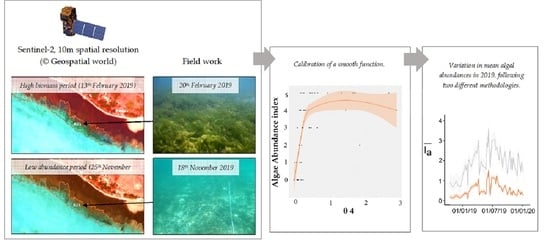
In 2014, the European Space Agency (ESA) started the Copernicus program and launched the two Sentinel-2 satellites, which supply since 2017 free data at 10-m resolution with a 5-day revisiting time. The Multi Spectral Instrument (MSI) used for this program offers an interesting trade-off between cost and spatial and temporal resolutions that should be more suitable than previous remote sensing commercial products for characterizing the dynamics of green algae blooms in tropical lagoons. Thus, Sentinel-2 brings new perspectives to monitor these events. Here, we tested the ability of Sentinel-2 imagery to characterize green macroalgae dynamics within a shallow coral reef lagoon in New Caledonia recently impacted by green tides. First, using images quasi-concurrent with field data, we fitted a relationship between in situ algal abundance and various radiometric indices calculated from Sentinel-2 MSI reflectances. Then, the best model was used to extrapolate algal dynamics over a three-year period, from January 2017 to December 2019. The method has been evaluated regarding its ability in capturing two documented
Ulva spp. blooms that occurred in 2018 and 2019 in the studied area [
27,
28].
2. Materials and Methods
2.1. Study Site
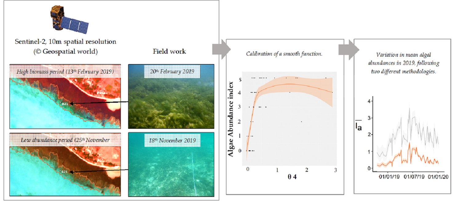
New Caledonia is a French overseas territory, located in the south-western Pacific Ocean, ~1500 km east of Australia (
Figure 1a). It comprises one main large island, known as Grande Terre, bordered by a 1600-km long barrier reef, which delimits a 23,400 km
2 lagoon [
29]. Due to their good health conditions and high biodiversity, six different areas, or clusters, of New Caledonia reefs and lagoons were listed as UNESCO World Heritage Areas in 2008 [
30]. New Caledonia is not spared from green tides, with occasional events of short duration recorded since 1996 in the bays near the town of Nouméa, and induced by the Japanese algae
Ulva ohnoi.
The present study focuses on the Poé-Gouaro-Deva (PGD) zone (21°37′10″S, 165°23′16″E) located on the west coast of Grande Terre. The studied area is located on the coastal area in the Bourail region, in the South Province of New Caledonia. It is bounded by the Gouaro reef in the southeast, and by the so-called Shark’s Fault (Faille aux requins) in the northwest. The area contains a Marine Protected Area (MPA) and is included in the UNESCO areas. The coral reef complex borders the coastline (
Figure 1b), forming a narrow (<3 km) and shallow lagoon (maximum depth ~4 m). Tides in this area can be classified as micro-tidal, mixed and mainly semi-diurnal, with a tidal range that can reach a maximum of 1.8 m during spring tide. The northwest part of the lagoon (~10 km
2) is mainly made of sandy soft-bottom habitat, while the southeast part (~9 km
2) is dominated by hard ground and coral communities and patch reefs. A several tens of meters-wide fringing seagrass bed (~3 km
2) borders the shoreline [
31]. This seagrass belt is not homogeneous and can be intertwined with patch of coral communities (branching
Montipora and
Acropora) and sand.
The PGD area is a hotspot of tourism activities, with increasing human pressures on the reef and lagoon ecosystems. Tourist frequentation has increased over recent years, with about 4000 Deva visitors in 2017 and more than 6500 in 2019 (data from Maison de Deva). Developing lands have also tripled in surface area from 1998 (~100 ha) to 2014 (~350 ha, [
32]). In early 2018, a green tide occurred in the PGD lagoon, with green macroalgae washed onshore in significant amounts on 18 January (~500 m
3 collected in three clean-up operations, Coutures personal observations), mostly along a 2.5-km long coastline located in the northwest part of the study zone (
Figure 1b). The algae decaying on the beach prevented tourism activities and could induce health threats. Another stranding event, although of a smaller intensity than the first event, impacted the beach on 1 June 2019.
2.2. In Situ Measurements of Algal Abundance
Field investigations were first carried out in February 2019 and May 2019, at 24 and 42 stations, respectively. Among the 24 stations visited in February 2019, most of them were revisited in May 2019. All stations were preliminarily selected using a remote sensing-driven site selection method, similar to that in Andréfouët and Wantiez (2010) [
33], to best capture the diversity of habitat in the area (seagrass bed, sand, coral reef and mixed habitats). For station selection, we used a multispectral Pléiades image ([
34], Airbus DS Geo distribution, resolution ~70 cm) dated from 17 July 2017.
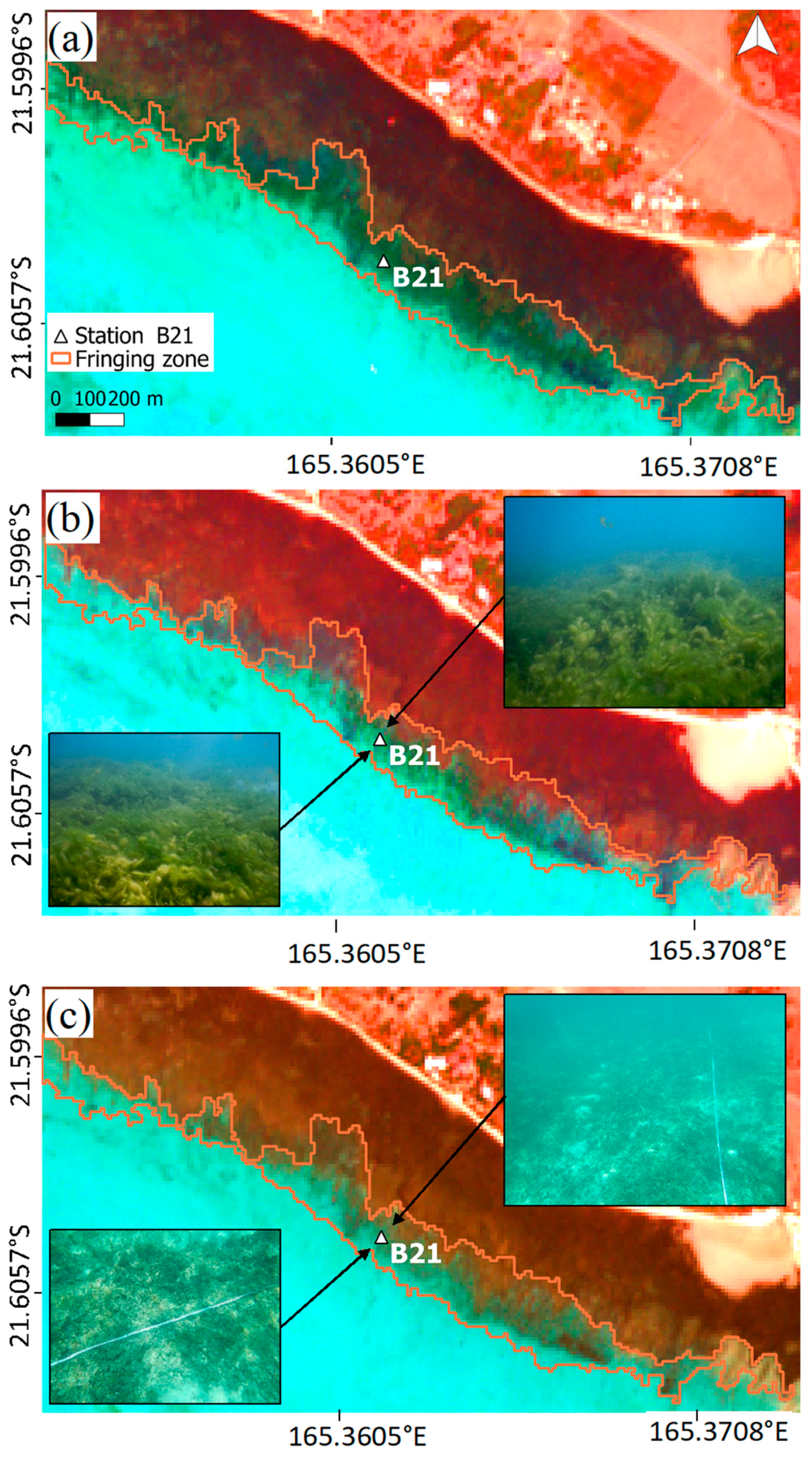
Second, three field trips took place in July 2019, September 2019 and November 2019, with a sampling dedicated to the monitoring of one single station (B21) where the biomass observed in February and May was particularly high (
Figure 2a,
Figure 3b).
Finally, 11 new additional stations were opportunistically sampled during 4 surveys dedicated to seawater samplings in December 2018, March 2019, July 2019 and October 2019. These stations did not specifically target areas with known past high abundances of green algae.
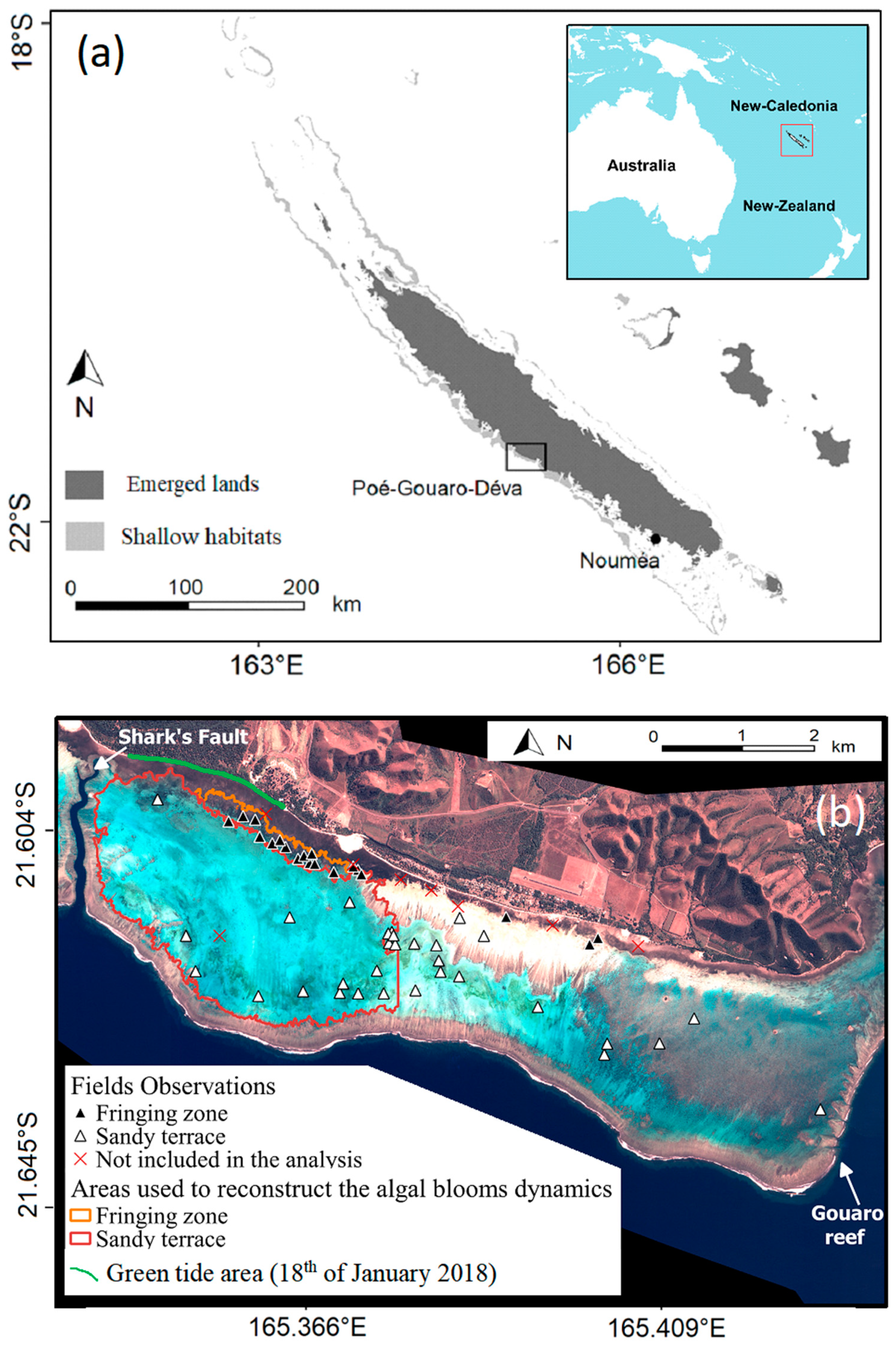
For each survey and each station, the cover of green algae was estimated semi-quantitatively using the Braun-Blanquet cover-abundance scale [
35], ranging from 0 (no green algae) to 5 (cover exceeding 75%) from wide-angle photos and videos taken during the field investigations (
Table 1;
Figure 2). The method is similar to the Medium-Scale Approach [
36] used to describe fish habitats using a semi-qualitative scale for each benthic descriptor. The results are estimates of green algae abundance (index
) at a scale compatible with the resolution of Sentinel-2 data (100 m
2 pixels, see next section). In total, 9 samplings campaigns carried out from December 2018 to November 2019 provided 97 measurements of green algae abundances, with 57 along the fringing and seagrass reef and 40 spread over the sandy terrace (
Figure 1b). This method was favored compared to a quantitative approach (using transects or quadrats) because it allows for covering a large area with more stations. Although this approach provided less precise estimates of algae abundance for each pixel individually, it could survey a large panel of pixels in different configurations.
2.3. Sentinel-2 Data Sets
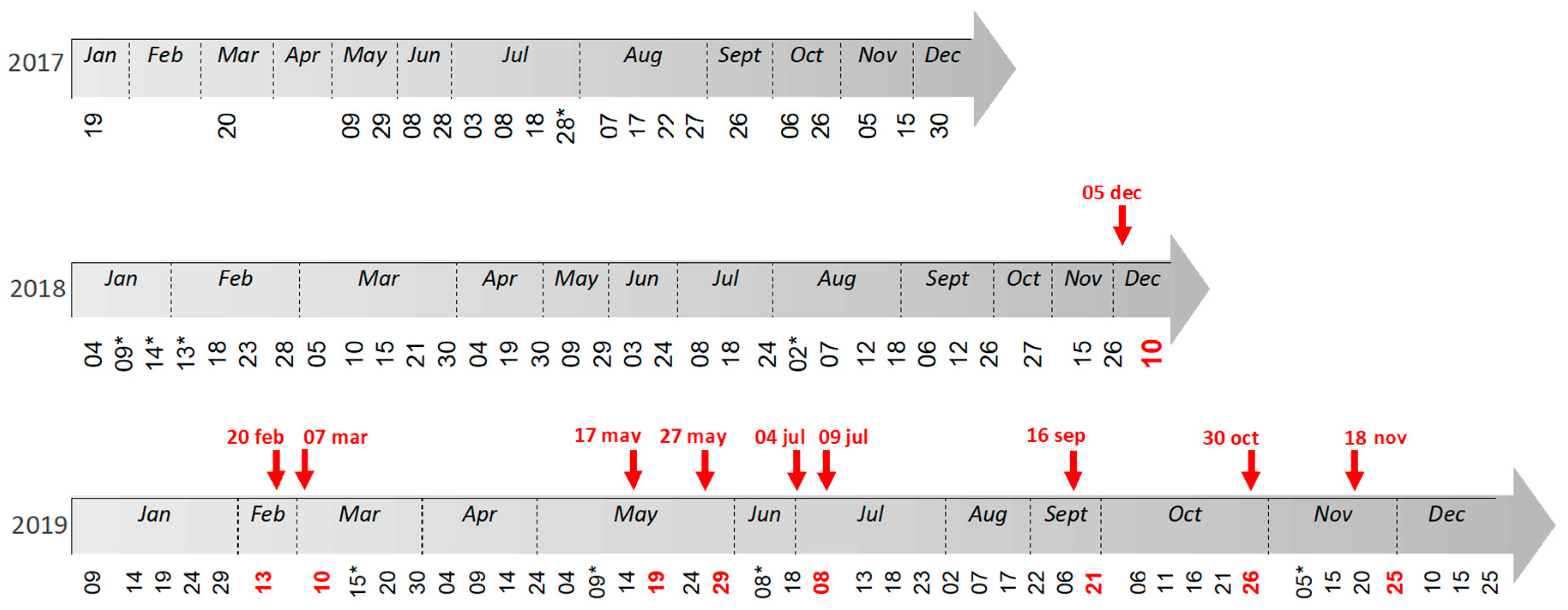
Cloud-free Sentinel-2 images (10 m resolution) available for the study area were retrieved from the Data Hub website (© Data Hub System 2.4.1, [
37];
Figure 4). Data downloads provided a time-series of images from 2017 to 2019. This consisted of Level 2A images (i.e., images corrected for the atmospheric signal) when available. Otherwise, Level 1C images (i.e., images without atmospheric correction) were used and were atmospherically corrected using the Sen2Cor processor from SNAP (© SNAP, 7.0) to create Level 2A products. This open-source program developed by the ESA provides surface, bottom of atmosphere (BOA) reflectance similar to the Level 2A products provided by the ESA/Copernicus program. Since we aim to apply statistical segmentation, classification and empirical correction to estimate algal abundance (see below), BOA reflectance was deemed adequate and no further correction was applied, for instance, to attempt to correct the air–water interface in the lagoon.
The Sentinel-2 MSI instrument measures reflected radiance in 13 spectral bands. Four of them have a 10-m spatial resolution, namely the blue (490 nm); green (560 nm); red (670 nm) and near-infrared (850 nm) bands. Only spectral bands in the blue (
B2) and in the green (
B3) zones were considered for this study, because red and especially near-infrared signals are attenuated quickly in the water column [
38].
Prior to performing a change detection analysis, two methods were implemented to empirically inter-calibrate BOA reflectance between images. These corrections used a Sentinel-2 image dated from 25 November 2019 as a radiometric reference because the concurrent field trip performed in this period (18 November 2019) highlighted a very low algal cover in the studied area (
Figure 3c). At the time of the analysis, the 25 November 2019 image was the closest in time available to this field trip. The first method (hereafter named “type 1 correction”) is an empirical band-to-band and image-to-image correction which required identifying, across the time-series, 105 pixels considered as pseudo-invariant features on the ground. The method relies on the hypothesis that the targeted objects (e.g., roads and roofs) are radiometrically invariant during the studied period. Any instability in the reflectance of these objects, therefore, can create biases due to environmental conditions (e.g., wetness on ground) or noise at the time of processing after image acquisition (resampling). To inter-calibrate the images, a band-specific linear relationship was built between the BOA reflectances of the pseudo-invariant features for each pair of images (reference image and image to be processed) using Equations (1) and (2) [
39].
where
a,
b,
c and
d are the coefficients of the linear relationships built from the pseudo-invariant pixels and
and
, the BOA reflectances of the spectral bands in the blue and the green.
The second correction aimed at minimizing the differences caused by the seabed composition (other than green macroalgae) within an image.
B2 and
B3 reflectances associated to each pixel were standardized following Equations (3) and (4). This correction was first applied alone (hereafter named “type 2 correction”), and we also applied this correction followed by the first one (“type 3 correction”).
where
and
are the BOA reflectances in the blue and the green bands, respectively, associated to the reference image (25 November 2019); and
and
are the arithmetic means of reflectance across all pixels associated to the field stations of this image. These constants were added to avoid generating negative radiometric values, which are not compatible with the calculation of some of the radiometric indices (cf. next section).
Note that correcting for co-registration errors was not performed in our study since the L1C processing chain already implements a geometric step which aims at improving the repetitiveness of the image geolocation in order to reach a multi-temporal geolocation target (<0.5 pixel at 95% confidence). When performing the type 1 correction, we could further confirm that the set of Sentinel-2 images we used was affected by negligible co-registration errors, since locations of the pseudo-invariant pixels were stable, and no offset of these pixels over time could be noticed.
2.4. Relationship Between Reflectance and Green Algae Abundances
To calibrate a biomass vs. reflectance (or spectral index, see below) relationship, for each sampling campaign the analysis was performed on the closest Sentinel-2 image in time. Offset between field work and image acquisition was always inferior to 7 days (
Figure 4). GPS measurements of the field stations were deemed precise at pixel resolution after comparison with remarkable features visible on ground and in images.
The blue and green BOA values were then used to compute six radiometric indices.
For the two types of substratum encountered in the study area, namely sandy bottoms vs. mix substrates along the fringing area (made of unconsolidated calcareous and terrigenous sand, coral and seagrass), the semi-quantitative abundance of green algae from field observations was expressed as a function of each radiometric index, using a non-parametric smooth function calibrated via the R studio mgcv package (©2009–2019 R studio v1.2.1578). The performance of the models was compared on the basis of the percentage of variance explained and using the generalized cross-validation (GCV) criteria.
2.5. Mapping of Green Algal Dynamics
We hindcasted the dynamics of green algae over the period covered by the Sentinel-2 imagery (from 19 January 2017 to 12 December 2019) for two shallow areas of interest in the PGD area (
Figure 1b). These areas were selected after field work considering they were prone to macroalgae proliferation or accumulation. The first area (hereafter named ‘the fringing area’; ≈48 ha) included very shallow (<2-m depth at low tide) stations located along the littoral in the west part of the lagoon. It is characterized by a mosaic of benthic components (seagrass, sand and corals). The second area (hereafter named ’the sandy terrace’; ≈780 ha) was also located in the west part of the lagoon but included stations located on the sandy terrace away from the littoral and in slightly deeper water (2–4 m deep at low tide).
For each area of interest, two different methods were tested to extrapolate the abundance of green algae. The first approach (hereafter ‘the unsupervised approach’) used the best fitted model selected in the previous section to predict, for each pixel located in the area of interest, the algal abundance (
Ia) from the
R(
B2) and
R(
B3) radiometric values. This was realized using the predict.gam function with the R studio mgcv package. The reconstruction of green algae dynamics was performed for the two areas of interest, computing, for each area, the arithmetic mean value of algae abundance per pixel (
) (Equation (9)).
where
n refers to the number of pixels in the area of interest.
The second approach (hereafter ‘the supervised approach’) involves a photo interpretation step. First, the two areas of interest were segmented in order to define homogeneous polygons in terms of blue and green radiometric values. The segmentation was performed using the automatized meanshift algorithm of the Orfeo ToolBox (OTB) plugin from QGIS software (© Qgis version 3.10.4). Then, algal-free polygons were visually identified by one of the authors (M.B.) and dismissed from the analysis. For each remaining polygon, an abundance-dominance green algae index was predicted, following the same procedure as for the unsupervised approach. The reconstruction of green algae dynamics was performed by computing, for each area of interest, the arithmetic weighted mean value of algae abundance associated to each polygon (
Ia), weighted by its surface area (Equation (10)).
where
n refers to the number of polygons in the area of interest and
Ai the surface area of polygon
i.
The various time-series of green algae abundances () obtained from the combination of different image inter-calibration procedures, spectral indices and mapping procedures were compared regarding their ability to reproduce the two green tides recorded in the study area in 2018 and 2019.
3. Results
3.1. Algal Diversity
Several species of green algae (Chlorophyta) have been observed in the different study areas in the lagoon, including Boodlea, Chaetomorpha, Cladophora and Ulva. Ulva was dominant, with several species having a filamentous and tubular morphology. A molecular taxonomical study currently being completed has shown the coexistence of four genetically different species. Three of them are attached to the substratum mainly in sandy areas, while the blooms consist of free-moving masses of strongly entangled filaments which accumulate along the coastline in the seagrass areas. The bloom-forming alga is a highly branched species of Ulva (Ulva sp3) which morphologically resembles Ulva prolifera but is genetically distinct from it. In some samples from the blooms, there could be several taxa (Boodlea and Cladophora), but most of the time, the dominant species was Ulva sp3.
3.2. In Situ Estimation of Algal Abundance
In February 2019, green algae were abundant (2 < Ia < 5) at two stations located in the fringing zone in the western part of the lagoon. Relatively high abundance-dominance indices (2 < Ia < 3) were also obtained for three stations on the sandy terrace. The abundance of algae was poor or null (Ia ≤ 1) at all other stations. In May 2019, the spatial distribution of green algae was similar to February 2019, with abundance-dominance indices from 0 to 4 at stations located in the sandy terraces and from 0 to 5 at stations located in the fringing zone. Along this area, a significant variability in abundance (0 < Ia < 5) was also found between stations during all of the 2019 surveys, except in November 2019, when abundance was low (Ia = 0) all across the fringing zone.
The wide range of Ia values across the different field surveys and stations allowed for calibrating a representative and robust relationship between Ia and the radiometric indices derived from remote sensing images (see next section).
3.3. Relationship between Radiometric Indices and Algal Abundance
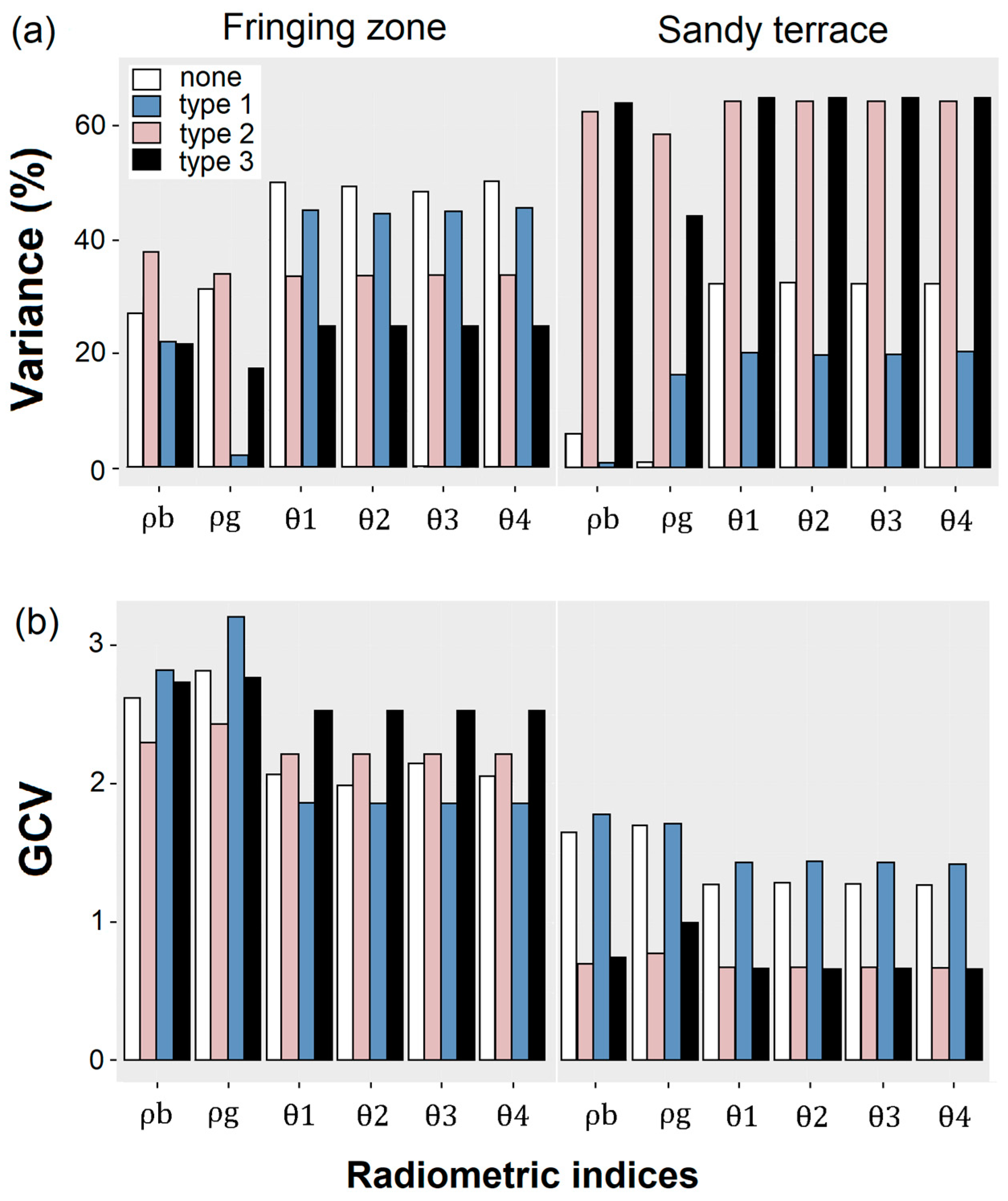
Without any correction applied (neither type 1, 2 nor 3), the multispectral indices
,
,
and
better explained variance than the ρ
b and ρ
g indices (
Figure 5). This trend was obtained both for stations located in the fringing zone (i.e., between 48.6% and 50.3% of variance explained by
,
,
and
vs. 27.2% and 31.5% of variance explained by ρ
b and ρ
g) and for stations located in the sandy zone stations (i.e., 32.3–32.5% vs. 6% and 1%).
For the stations located on the sandy terrace, the type 2 and 3 corrections improved the goodness-of-fit test results (
Figure 5). Specially for the
index, the explained variance increased from 32.3% without correction to 64.3% with type 2 correction and to 64.9% with type 3 correction. However, applying the type 2 or the type 3 correction degraded the fit for the fringing zone (
Figure 5).
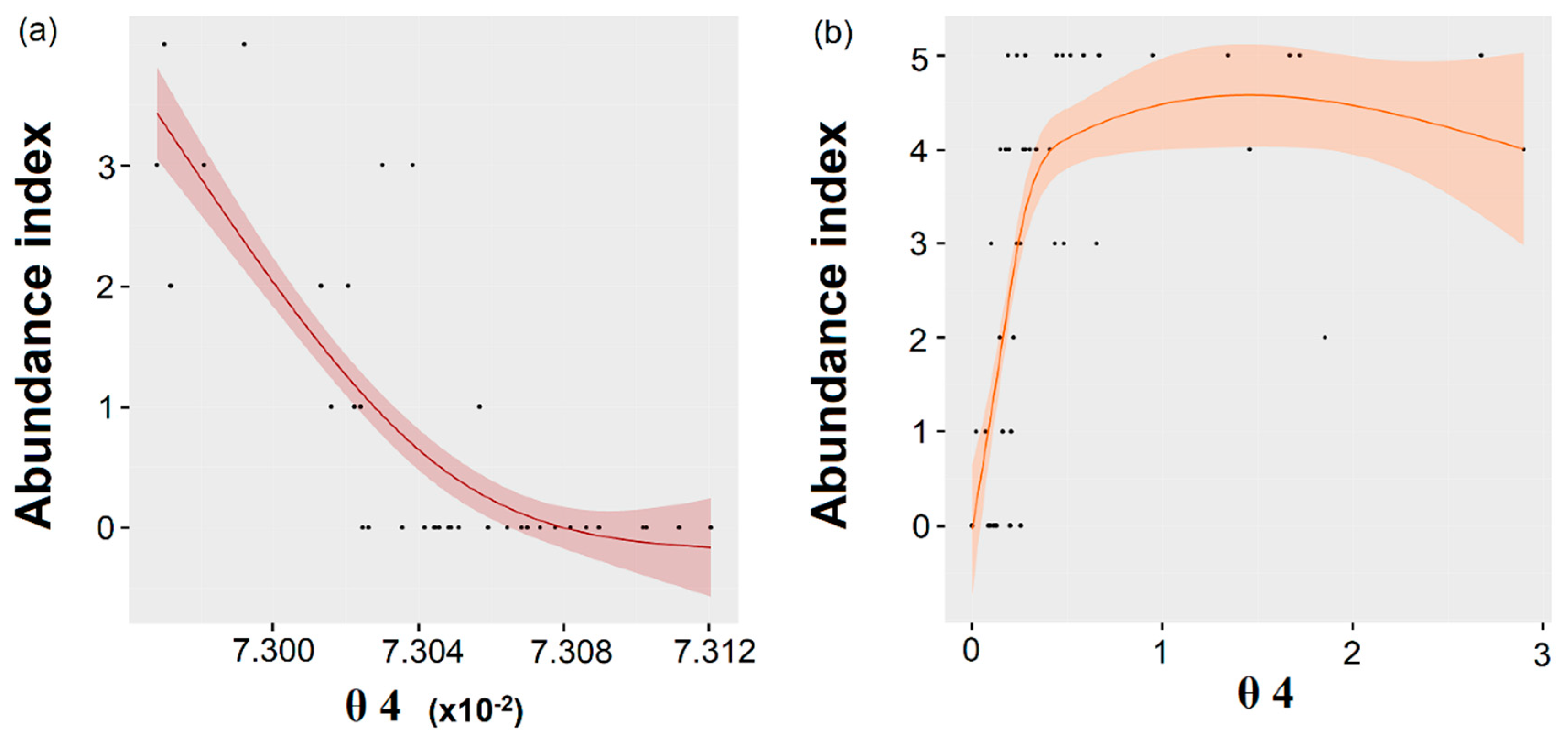
Eventually, the
index based on
R(
B2) and
R(
B3) without any corrections provided the best model for the fringing zone (i.e., 50.3% of variance, GCV = 2.06,
Figure 6b). For the sandy terrace,
also provided the best model (i.e., 64.9% of variance, GCV = 0.66,
Figure 6a) but only when the type 3 correction was applied (
Figure 5). These indices and correction types were therefore selected to extrapolate the algal abundance across the Sentinel-2 time-series (next section).
3.4. Mapping and Dynamics of Green Algae Abundances Using Sentinel-2
For the fringing area, using the supervised approach always yielded lower
values than with the unsupervised approach (
= 0.63 on average over the period of 2017–2019 against 2.00;
Figure 7a). Despite this difference, both approaches could identify the January 2018 and June 2019 algal blooms, both producing significant macroalgae pile-ups on the beach. The abundance variations hindcasted on the sandy terrace area were not always synchronous with those hindcasted in the fringing area. Unlike the fringing zone, the supervised and unsupervised approaches were more in agreement to each other in this habitat (
Figure 7b). The dynamics of green algae hindcasted for both areas by the supervised and unsupervised approaches suggested high algal abundance throughout the year, except during the dry season (October and November;
Figure 7). In particular, periods of high algal abundance were predicted around July 2017, July 2018 and July 2019 for both fringing and sandy terrace areas, although no green tide was reported, to our knowledge, during these periods.
4. Discussion
4.1. Innovative Nature of the Approach and Proposed Method
This paper demonstrates that the Sentinel-2 imagery is a valuable tool to hindcast the dynamics of benthic green algae in shallow coral reef lagoons, which is required to understand the causes of the algal tides when confronted with other data sets (e.g., lagoon temperature; solar irradiance; rainfall or streamflow from nearby rivers). Here, we focused on the benthic biomass of green macroalgae during blooming conditions in a shallow lagoon. This is in contrast with most recent remote sensing studies which looked at green and brown algae once they had beached and algal rafts while drifting on the ocean surface [
16,
17,
18,
19,
20,
21].
To date, most of the multispectral indices proposed in the literature for detecting macroalgae used the red visible and/or near-infrared bands [
19,
20,
23,
45,
46,
47]. These spectral bands have been commonly used because they are suitable to capture chlorophyll absorption peaks and the overall vegetation spectral signature when it is above water or just at the ocean surface. The NDVI, which uses a ratio of the red visible and near-infrared bands, has been widely used as an indicator of floating algae mats’ presence/absence [
20,
48,
49,
50]. The NDVI has also been used successfully for mapping and monitoring phanerogams [
51]. Despite the potential of the red and near-infrared bands to distinguish vegetation, these radiations are quickly attenuated in water, and spectral indices based on these bands are very sensitive to depth variations, either due to bathymetry or tide [
52,
53]. For instance, Andréfouët et al. [
26] showed that even in a low-depth environment (<2 m), red and near-infrared bands were not ideal to map the biomass of benthic
Sargassum polycystum brown algae. Although the index of floating algae based on the red and near-infrared bands may be useful to identify the presence of green algae in their final floating cycle, this index was of low interest in our case study, because the floating phase of algae’s life cycle is very short and was never observed during field work. This made NDVI a poor proxy of algal abundance in our case study (
Figure S1). In this paper, a modified version of the NDVI, switching the red and infrared bands with blue and green bands, provided more conclusive results to quantify the abundance of benthic green algae. This agreed with previous studies that used NDVI-like indices with a variety of band combinations [
53,
54].
In our study, multispectral radiometric indices (i.e.,
,
,
and
) provided more convincing results than the green band alone (i.e., ρ
g). These findings are in contrast with the work of Andréfouët et al. [
26] for
S. polycystum in an atoll lagoon. For this brown alga, the green band provided a fit with biomass nearly as good as our multispectral indices and was used to hindcast its dynamics from 2002 to 2015 using a range of high-resolution remote sensing images (QuickBird 2, IKONOS, WorldView-2, Pléiades 1B, 1A).
4.2. Influence of the Three Types of Corrections
Using the type 1 empirical approach alone to correct the radiometric data was found to be of limited interest. Two explanations can be provided. First, our study relied on images that were corrected beforehand with an ESA model in order to remove the atmospheric signal. It implies that the additional type 1 correction provided no added value to monitor the green algal proliferation, compared to using L2A images. This might be the result of using imperfect pseudo-invariant features for this correction. However, models and algorithms automatically used to correct the entire L1C images are unlikely to be enough to perfectly correct the images locally in our studied areas of interest [
55,
56]. Specifically, for coral reef areas, local processes can affect the atmospheric signal quality, such as ocean spray induced by waves breaking on the reef ridge.
Secondly, previous studies already highlighted the limits of the type 1 correction for areas of high algal biomass. High biomass is correlated with low radiometric value (in the green band, or for a given radiometric index [
26]). Indeed, in such a configuration, the relationship applied to estimate biomass is very sensitive because a wide range of biomass corresponds to a narrow radiometric range. However, the type 1 correction for intercalibrating images is easily applicable to coastal areas where remarkable pixels can be precisely identified in all the images acquired on different dates [
39].
To our knowledge, the type 2 processing proposed in this paper has never been documented before. It provided relevant results for the sandy terrace, which is made of relatively homogeneous pixels. In contrast, the type 2 correction turned out to be inefficient in the fringing zone. This result may partly be explained by tide, which may affect Equations (3) and (4) with stronger intensity in the fringing area, shallower than the sandy terrace area. Moreover, the heterogeneity of the fringing area, which is a mix of sand, corals and seagrasses, may also contribute to the poor performance of type 2 correction. Indeed, pixel resampling and misregistration may affect the signal to a greater extent in this heterogeneous area than in the sandy area. Implementing a co-registration method to correct errors and align pixels between images could be beneficial for future case-studies when the habitat is highly heterogeneous.
4.3. Supervised vs. Unsupervised Approach
The supervised and unsupervised approaches tested in this study to hindcast the algal dynamics offer different levels of cost effectiveness. Concerning ‘costs’ (in terms of time and expertise), the unsupervised method only involves a quick QGIS manipulation of a few minutes per image and does not require any specific expertise. The supervised approach, by contrast, requires the capacity to identify the presence/absence of algal mats on Sentinel-2 images, an expertise acquired by comparing field observations concurrent with images. The method also requires a longer analysis time (i.e., ~20 min per image for the PGD area). The cost depends on the surface area to process and can be significant for large lagoons. Although the unsupervised approach does not require any expertise (beside understanding the software), the processing time (using R software) associated to this approach increases exponentially with the number of pixels. For the entire PGD area (fringing zone and sandy terrace zone confounded, assembling 94,202 pixels), the algorithm takes about 1 h to complete (computer with 8192 Mo usable RAM and ~1.8 GHz processor). This may impair, for larger areas, the feasibility of real-time processing to anticipate beach stranding events. By contrast, following the interactive part, the processing time using R software associated to the supervised approach only takes a few minutes to complete, regardless of the size of the area, as it manipulates vectors (i.e., polygons) of several hectares instead of 100 m2 pixels raster data.
Regarding the accuracy of estimations, the supervised approach allowed to discriminate the two bloom periods which led to beach stranding events in the PGD area. The unsupervised approach, by contrast, could not identify these specific events. The unsupervised approach also overestimated the average algal abundance () over the study period (i.e., from 2017 to 2019). Indeed, the field survey carried out in November 2019 reported a fringing zone free of algae, while the algal abundance hindcasted on the reference image by the unsupervised approach was high (mean value equal to 2.39). The supervised approach, on the other hand, provided more plausible estimates ( = 0.53 on 25 November 2019). We thus recommend the supervised approach over the unsupervised one when the time and level of expertise are not constrained.
4.4. Tracking the Origin of Green Tides
The abundance of green algae estimated using Sentinel-2 data enabled identifying a bloom of algae located in the fringing area before the beach stranding event reported at PGD in January 2018. Therefore, the hindcast of algal dynamics performed in this study provides clues to identify the main pathways of nutrients that induced this event. Indeed, to implement management actions, local stakeholders lacked evidence on whether the stranding event recorded at PGD in front of the fringing area was induced by an input of nutrients very locally or if it was the result of the drift of algae biomass that originated elsewhere. Here, we provide evidence of the existence of a peak of algal abundance on the fringing area starting several weeks before the beaching event. By contrast, the abundance hindcasted in the sandy terrace before the beach stranding event of 18 January 2018 is quite low (
< 1 for both approaches, see
Figure S2). These results suggest that this stranding event was mainly due to algae biomass from the fringing zone. This hypothesis is consistent with the identification of two distinct species of
Ulva genus in the PGD lagoon, which respectively dominate the sandy terrace and the fringing area [
27,
28]. The morphology of the species dominating the fringing area (i.e., forming dense unattached mats of long filamentous thallus) is more likely to generate green tides compared to the species that dominates the sandy terrace (species forming a smaller thallus attached to the substratum) [
27,
28].
It is worth noting that to track the origin of green tides in the PGD lagoon, we here developed an approach slightly different than those implemented in previous remote sensing studies for monitoring green macroalgae proliferations. Indeed, as previous studies focused on floating algae while drifting on the ocean surface, they aimed at developing methods that can detect these mats across wide areas of oceanic waters [
16,
17,
18,
19,
20]. By contrast, the framework developed here aimed at hindcasting algae abundance in small areas suspected to experience green tides. Although this new framework requires sufficient knowledge on suitable habitats for algae and potential sources of nutrient to identify a priori the area that will be monitored, it is more relevant for monitoring blooms in small lagoons, where the rafting phase before beaching can be very brief and very spatially restricted within the lagoon.
4.5. Predicting the Risk of Beach Stranding Events
This study reconstructed the dynamics of green algae almost continuously over a three-year period. Similar objectives are not possible from in situ data. Although the fringing zone in the PGD lagoon is quite small and easily accessible from the beach, monitoring green algae cover in situ on a regular basis and in the long run turned out to be difficult to implement in practice, and using remote sensing is an attractive option. Eventually, we provided an indicator of risk for beach stranding events based on the estimates of green algal abundance (
), via the supervised approach, with a 5-day periodicity (assuming favorable cloud cover). The dynamics reconstructed in this study over the period 2017–2019, with two significant bloom periods, can be used to set threshold values for
, beyond which appropriate management actions may be needed (
Table 2). Notably, the beaching risk can be considered as null when
in the fringing area is lower than 0.53, which is, as on 25 November 2019, the predicted value at the time of very low algal abundance confirmed in the field (
Figure 3c). This baseline value, which is not equal to zero, corresponds to a background noise due to the various processing steps. Conversely, the beach stranding risk can be considered high when 1.13 <
< 1.86, thus, as in conditions observed in January 2018 and June 2019. In such cases, management actions can be preconceived to prevent and minimize the pile-up of algae on the beach (
Table 2).
Among the management actions that are recommended in case of moderate, high or extreme risk forecasted by the near real-time remote sensing protocol, we suggest (1) the implementation of, ideally, daily monitoring of algal cover along the fringing zone. This is recommended because the periodicity of the Sentinel-2 imagery (i.e., 5 days, assuming cloud-free weather) may be insufficient to accurately characterize the short-term evolution of each bloom. A second action recommended is (2) to plan clean-up measures on the beach. The removal of algae biomass accumulated along the shore is essential in order to avoid degradation of algae under anaerobic conditions and release of hydrogen sulfide. Finally, a third action that could be considered here in case of extreme risk of stranding events is (3) to remove a significant amount of macroalgae from the areas propitious to their growth (e.g., through field collection) in order to slow down the growth of the population. Although this action has already proven its efficiency to get rid of an already-formed bloom of green macroalgae [
9], it seems difficult to implement in the PGD fringing zone without significantly damaging the coral reef and seagrass habitats.
Despite that the Sentinel-2 missions are expected to end in 2024, the development of such an indicator of risk for beach stranding events using this imagery is a promising path for environmental management. Indeed, the ESA agency has mentioned a possible 5-year extension of their products with new satellites to be launched, thus ensuring an access to Sentinel-2 imagery until 2029. Beyond the Sentinel-2 imagery, one can also expect the launch of new missions providing products at higher temporal and/or spatial resolution, which should also provide relevant data for monitoring green macroalgae blooms in shallow lagoons.
4.6. Generalization to Other Lagoons in New Caledonia
In this study we demonstrated the potential of using Sentinel-2 images to monitor green macroalgae proliferation in the PGD shallow lagoon. Statistical relationships established between the
radiometric index and the green algae abundances, as well as radiometric corrections recommended for this study, were zone-sensitive (
Figure 5 and
Figure 6). Even though the shallow habitats, either fringing or part of the barrier reef complex, represent wide areas at the New Caledonia scale (
Figure 1), the PGD lagoon is quite an uncommon feature in New Caledonia due to its shallow depth and geomorphology [
29,
31]. The optical signature of the bands may vary from one site to another, depending on various parameters, including bathymetry, substrate nature, benthic components other than macroalgae and water quality. The diversity of these features is high in New Caledonia, and more work is needed at other sites to test the robustness of the methods established here.
Specifically for water quality, performing water column correction was not justified in our study since phytoplankton blooms were of lower concern in the PGD lagoon. Indeed, considering the shallow depths (between ~1.5 and 4 m) and low chl-a concentration in our study area (from 0.17 mg.m
−3 after a dry period to 0.75 mg.m
−3 after a heavy rain event, unpublished data), the decay of light along the water column remains fairly acceptable for the blue and green bands [
57]. Moreover, the spatial patterns of algae blooms that can be observed on the imagery followed the benthic features of the area (
Figure 3), indicating that the measured optical changes were driven by benthic algae, not by phytoplankton blooms. Finally, among all the methods developed to date for water column correction, none are capable of completely eliminating the water column effect [
57]. All methods require some inputs that were not available with sufficient accuracy in our study area, and some others make assumptions not supported in our study site. As a result, performing a water column correction with available data was likely to induce more bias in the analysis. Applying the framework developed for PGD to other sites may, however, require an additional step of water column correction, especially for lagoons characterized by higher chl-a concentration or deeper habitats than studied here. Note that such an additional step is not trivial, as it may require the acquisition of specific data for model input, including accurate depth or bathymetric maps, or high-resolution maps of substrate and knowledge on the spectral behavior of each substrate type [
57].

 ,
, 


