MorphEst: An Automated Toolbox for Measuring Estuarine Planform Geometry from Remotely Sensed Imagery and Its Application to the South Korean Coast

 , , ,
, , ,
Abstract
:
1. Introduction
2. Material and Methods
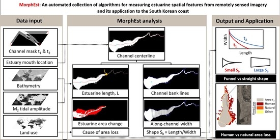
2.1. MorphEst
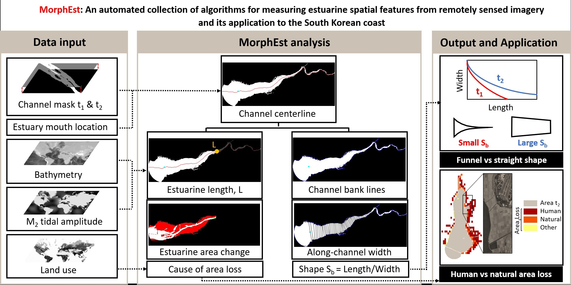
2.1.1. MorphEst Overview
2.1.2. MorphEst Input
2.1.3. Extraction of Channel Centerline
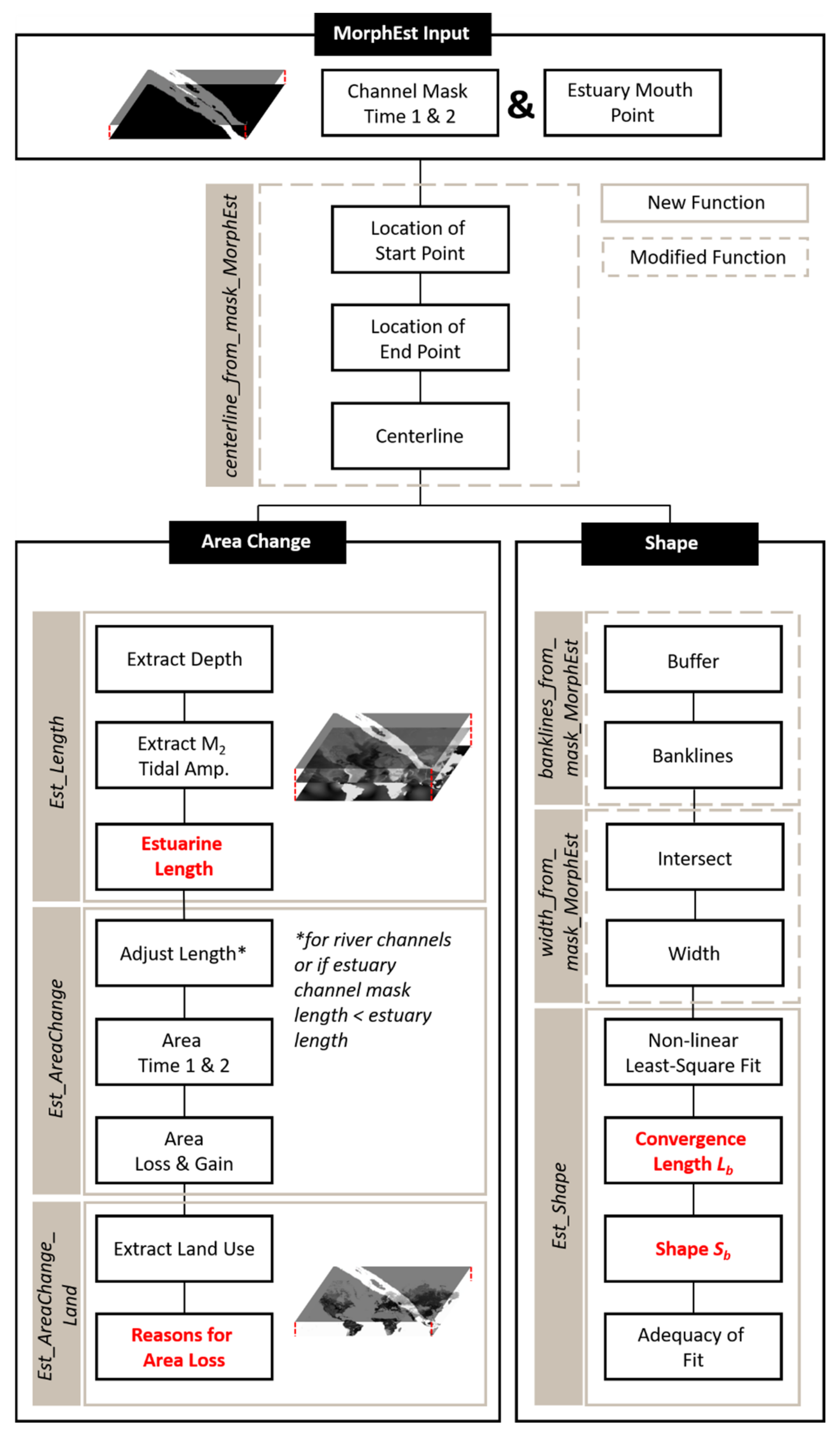
2.1.4. Calculation of Estuarine Surface Area Change between Two Time Intervals
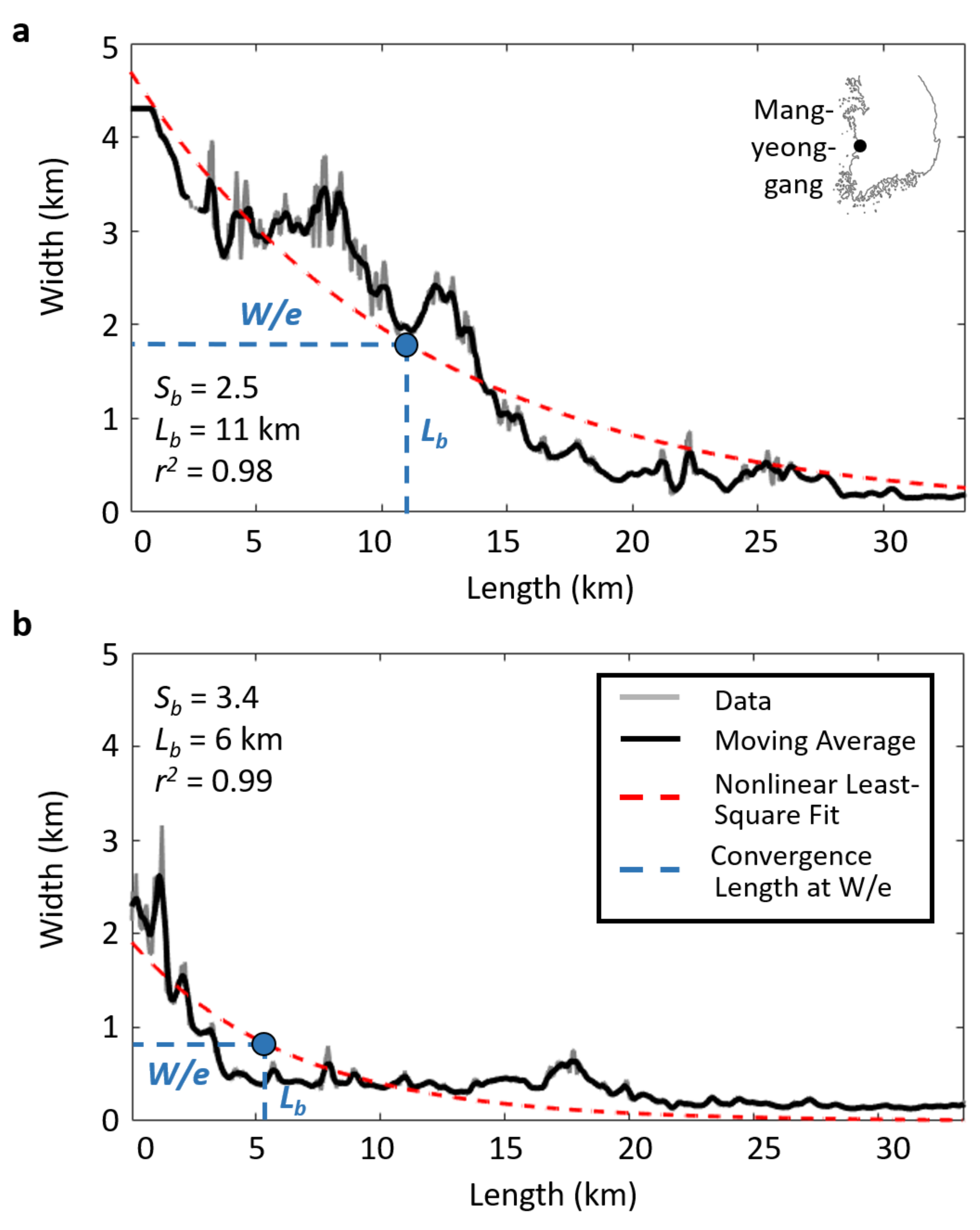
2.1.5. Measuring Estuarine Convergence Length and Shape
2.1.6. MorphEst Output
2.2. MorphEst Validation
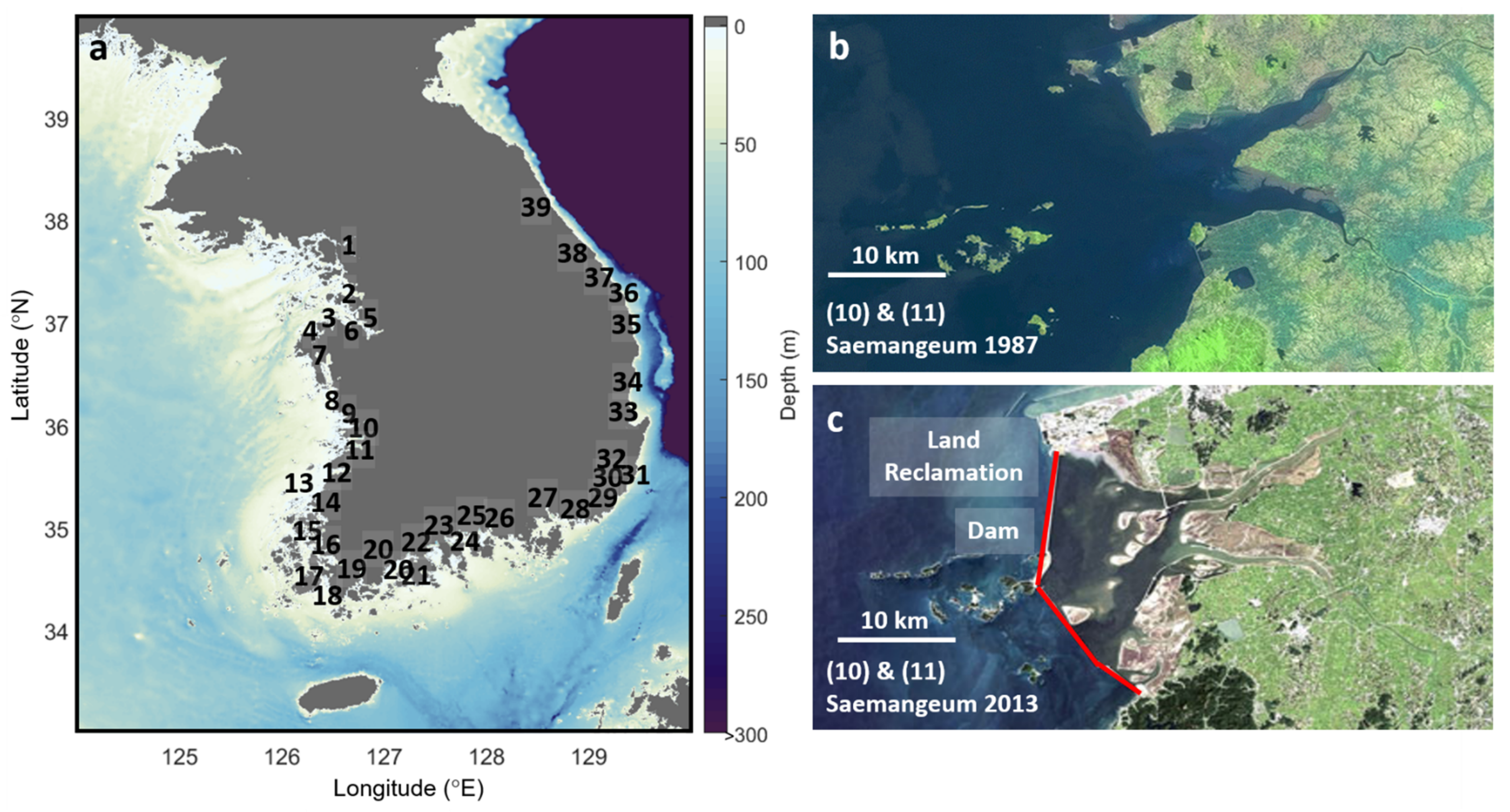
2.2.1. Study Area
2.2.2. Data Preparation
2.2.3. Error and Sensitivity Analysis
3. Results
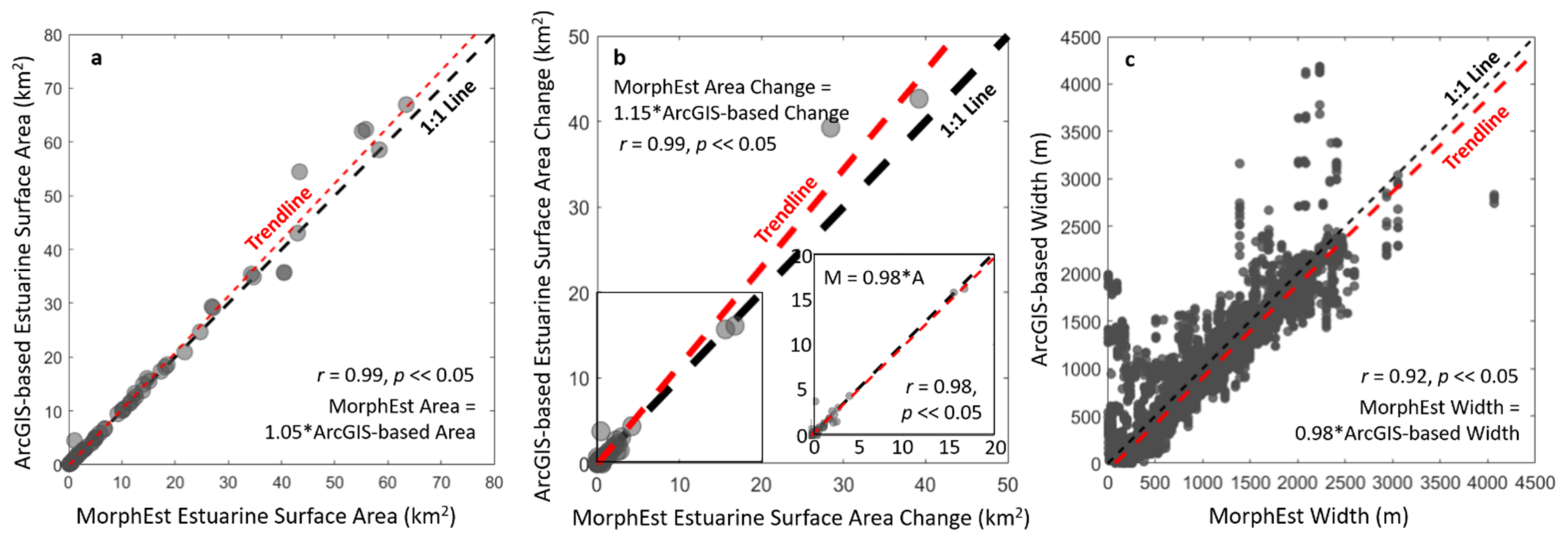
3.1. Validation and Sensitivity of MorphEst Measurements
3.2. Surface Area Change of South Korean Estuaries between 1985 and 2015
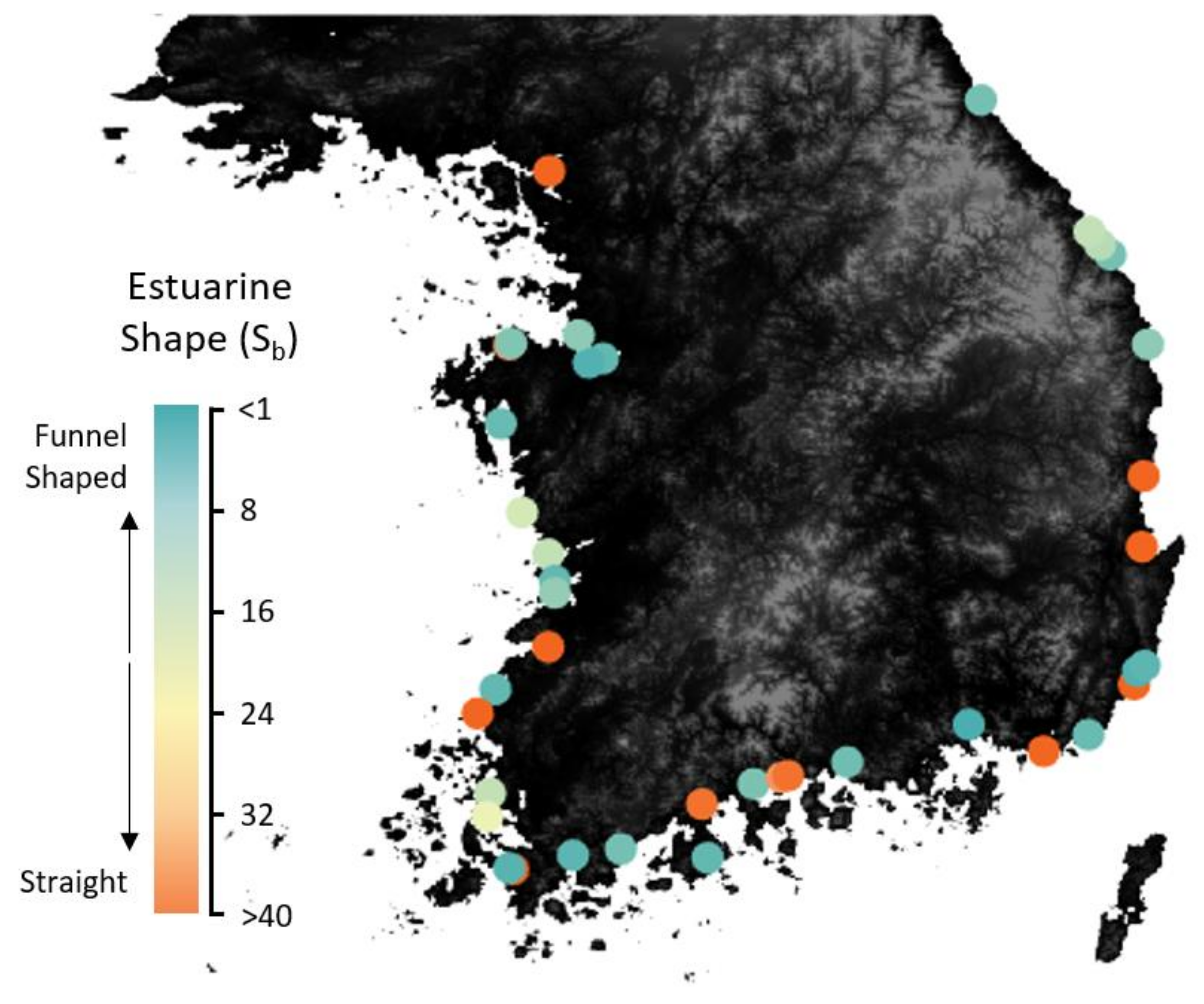
3.3. Shape Distribution of South Korean Estuaries
4. Discussion
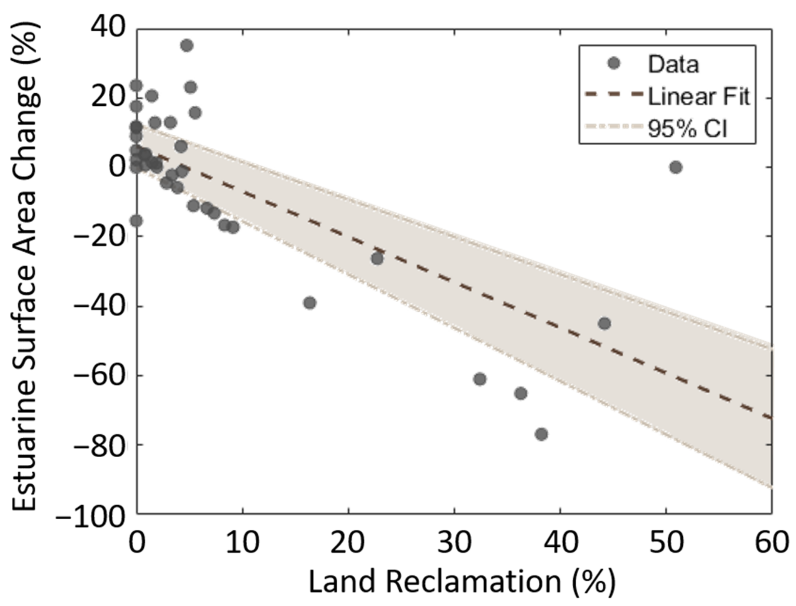
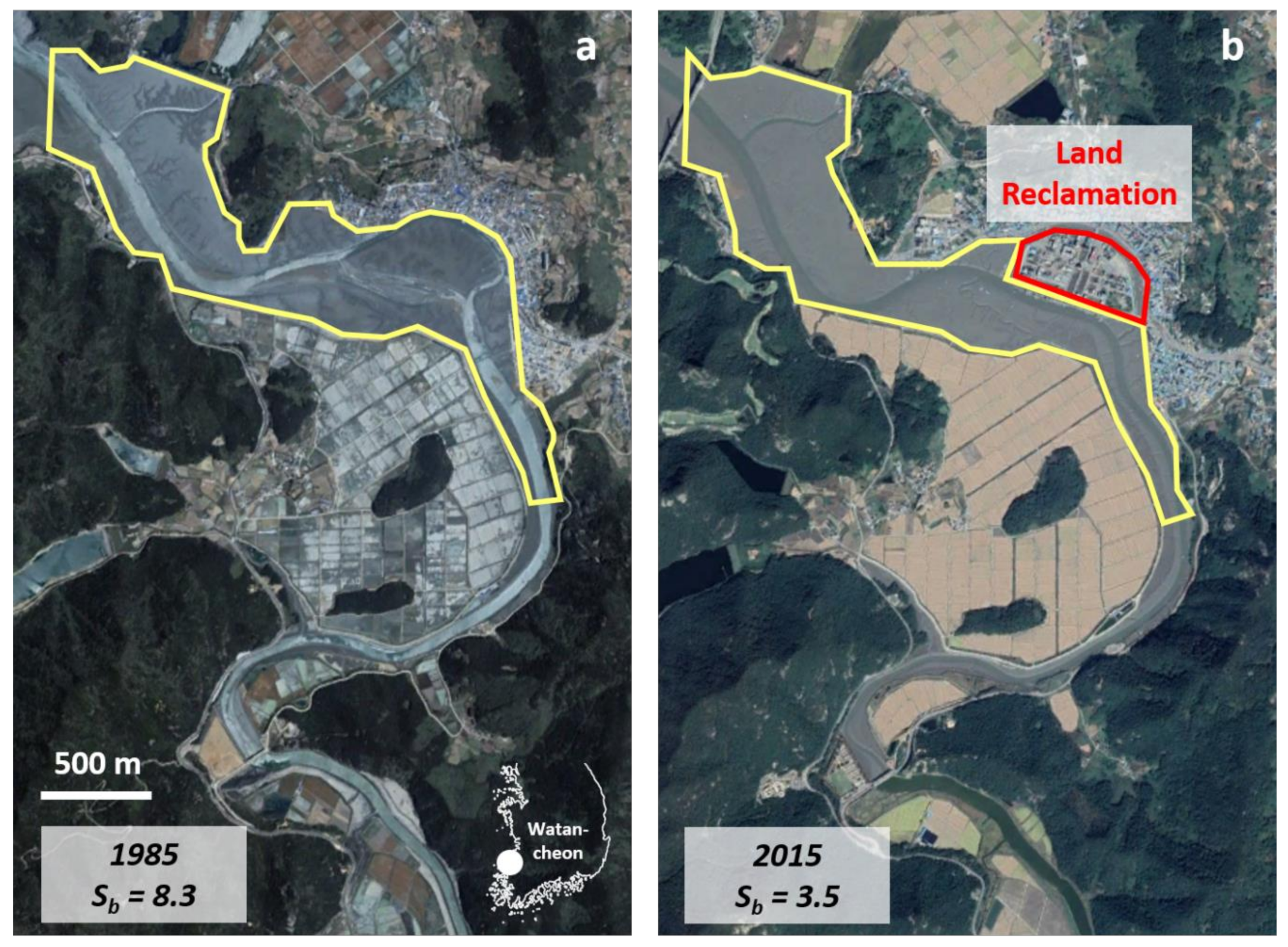
4.1. Land Reclamation as Main Driver of Estuarine Surface Area Loss
4.2. Human Impacts on the Shape of South Korean Estuaries
4.3. Future Research
5. Conclusions
Supplementary Materials
Author Contributions
Funding
Acknowledgments
Conflicts of Interest
References
- Kennish, M.J. Environmental threats and environmental future of estuaries. Environ. Conserv. 2002, 29, 78–107. [Google Scholar] [CrossRef]
- McGranahan, G.; Balk, D.; Anderson, B. The rising tide: Assessing the risks of climate change and human settlements in low elevation coastal zones. Environ. Urban. 2007, 19, 17–37. [Google Scholar] [CrossRef]
- Lotze, H.K.; Lenihan, H.S.; Bourque, B.J.; Bradbury, R.H.; Cooke, R.G.; Kay, M.C.; Kidwell, S.M.; Kirby, M.X.; Peterson, C.H.; Jackson, J.B.C. Depletion, degradation, and recovery potential of estuaries and coastal seas. Science 2006, 312, 1806–1809. [Google Scholar] [CrossRef]
- Cooper, J.A.G. Anthropogenic impacts on estuaries. In Coastal Zones and Estuaries; Ignacio, F., Iribarne, O., Eds.; Eolss Publishers Co Ltd.: Oxford, UK, 2009; p. 523. [Google Scholar]
- Byun, D.S.; Wang, X.H.; Holloway, P.E. Tidal characteristic adjustment due to dyke and seawall construction in the Mokpo Coastal Zone, Korea. Estuar. Coast. Shelf Sci. 2004, 59, 185–196. [Google Scholar] [CrossRef]
- Syvitski, J.P.M.; Vörösmarty, C.J.; Kettner, A.J.; Green, P. Impact of humans on the flux of terrestrial sediment to the global coastal ocean. Science 2005, 308, 376–380. [Google Scholar] [CrossRef] [PubMed]
- Walling, D.E. Human impact on land-ocean sediment transfer by the world’s rivers. Geomorphology 2006, 79, 192–216. [Google Scholar] [CrossRef]
- Wang, Y.; Dong, P.; Oguchi, T.; Chen, S.; Shen, H. Long-term (1842–2006) morphological change and equilibrium state of the Changjiang (Yangtze) Estuary, China. Cont. Shelf Res. 2013, 56, 71–81. [Google Scholar] [CrossRef]
- Williams, J.; Dellapenna, T.; Lee, G. Shifts in depositional environments as a natural response to anthropogenic alterations: Nakdong Estuary, South Korea. Mar. Geol. 2013, 343, 47–61. [Google Scholar] [CrossRef]
- Prandle, D. Estuaries: Dynamics, Mixing, Sedimentation and Morphology; Cambridge University Press: Cambridge, UK, 2009. [Google Scholar]
- Church, J.A.; Clark, P.U.; Cazenave, A.; Gregory, J.M.; Jevrejeva, S.; Levermann, A.; Merrifield, M.a.; Milne, G.A.; Nerem, R.S.; Nunn, P.D.; et al. Sea Level Change; PM Cambridge University Press: Cambridge, UK, 2013. [Google Scholar]
- Morris, R.K. Geomorphological analogues for large estuarine engineering projects: A case study of barrages, causeways and tidal energy projects. Ocean Coast. Manag. 2013, 79, 52–61. [Google Scholar] [CrossRef]
- Kidd, I.M.; Fisher, A.; Chai, S.; Davis, J.A. A scenario-based approach to evaluating potential environmental impacts following a tidal barrage installation. Ocean Coast. Manag. 2015, 116, 9–19. [Google Scholar] [CrossRef]
- Kench, P.S. Geomorphology of Australia estuaries: Review and prospect. Austral. Ecol. 1999, 24, 367–380. [Google Scholar] [CrossRef]
- Van der Wal, D.; Pye, K.; Neal, A. Long-term morphological change in the Ribble Estuary, northwest England. Mar. Geol. 2002, 189, 249–266. [Google Scholar] [CrossRef]
- Tanaka, H.; Nguyen, X.T.; Makoto, U.; Ryutaro, H.; Eko, P.; Mano, A.; Udo, K. Coastal and estuarine morphology changes induced by the 2011 Great East Japan Tsunami. Coast. Eng. 2012, 54, 1250010. [Google Scholar] [CrossRef]
- Mulligan, R.P.; Mallinson, D.J.; Clunies, G.J.; Rey, A.; Culver, S.J.; Zaremba, N.; Leorri, E.; Mitra, S. Estuarine responses to long-term changes in inlets, morphology, and sea level rise. J. Geophys. Res. Ocean. 2019, 124, 9235–9257. [Google Scholar] [CrossRef]
- Chang, J.; Lee, G.; Harris, C.K.; Song, Y.; Figueroa, S.M.; Schieder, N.W.; Lagamayo, K.D. Sediment transport mechanisms in altered depositional environments of the Anthropocene Nakdong Estuary: A numerical modeling study. Mar. Geol. 2020, 430, 106364. [Google Scholar] [CrossRef]
- Figueroa, S.M.; Lee, G.; Chang, J.; Schieder, N.W.; Kim, K.; Kim, S.-Y. Evaluation of along-channel sediment flux gradients in an Anthropocene estuary with an estuarine dam. Mar. Geol. 2020, 429, 106318. [Google Scholar] [CrossRef]
- Wright, L.D.; Coleman, J.M. Variations in morphology of major river deltas as functions of ocean wave and river discharge regimes. AAPG Bull. 1973, 57, 370–398. [Google Scholar]
- Galloway, W.D. Deltas, Models for Exploration; Broussard, M.L., Ed.; Houston Geological Society: Houston, TX, USA, 1975; pp. 86–98. [Google Scholar]
- Gisen, J.I.A.; Savenije, H.H.G. Relationship between estuary shape and hydrodynamics in alluvial estuaries. Geophys. Res. Abstr. 2012, 14, EGU2012–EGU2550. [Google Scholar]
- Nienhuis, J.H.; Ashton, A.D.; Giosan, L. What makes a delta wave-dominated? Geology 2015, 43, 511–514. [Google Scholar] [CrossRef] [Green Version]
- Nienhuis, J.H.; Hoitink, A.J.F.; Tornqvist, T.E. Future change to tide-influenced deltas. Geophys. Res. Lett. 2018, 45, 3499–3507. [Google Scholar] [CrossRef] [Green Version]
- Nienhuis, J.H.; Ashton, A.D.; Edmonds, D.A.; Hoitink, A.J.F.; Kettner, A.J.; Rowland, J.C.; Törnqvist, T.E. Global-scale human impact on delta morphology has led to net land area gain. Nature 2020, 577, 514–518. [Google Scholar] [CrossRef] [PubMed]
- Davies, G.; Woodroffe, C.D. Tidal estuary width convergence: Theory and form in North Australian estuaries. Earth Surf. Process. Landf. 2010, 35, 737–749. [Google Scholar] [CrossRef]
- Wolanski, E.; Moore, K.; Spagnol, S.; D’Adamo, N.; Pattiaratchi, C. Rapid, human-induced siltation of the macro-tidal Ord River Estuary, Western Australia. Estuar. Coast. Shelf Sci. 2001, 53, 717–732. [Google Scholar] [CrossRef]
- Pye, K.; Blott, S.J. The geomorphology of UK estuaries: The role of geological controls, antecedent conditions and human activities. Estuar. Coast. Shelf Sci. 2014, 150B, 196–214. [Google Scholar] [CrossRef]
- Bourman, R.P.; Murray-Wallace, C.V.; Belperio, A.P.; Harvey, N. Rapid coastal geomorphic change in the River Murray Estuary of Australia. Mar. Geol. 2000, 170, 141–168. [Google Scholar] [CrossRef]
- Blott, S.J.; Pye, K.; Van der Wal, D.; Neal, A. Long-term morphological change and its causes in the Mersey Estuary, NW England. Geomorphology 2006, 81, 185–206. [Google Scholar] [CrossRef]
- Luan, H.L.; Ding, P.X.; Wang, Z.B.; Ge, J.Z.; Yang, S.L. Decadal morphological evolution of the Yangtze Estuary in response to river input changes and estuarine engineering projects. Geomorphology 2016, 265, 12–23. [Google Scholar] [CrossRef]
- Murray, N.J.; Clemens, R.S.; Phinn, S.R.; Possingham, H.P.; Fuller, R.A. Tracking the rapid loss of tidal wetlands in the Yellow Sea. Front. Ecol. Environ. 2014, 12, 267–272. [Google Scholar] [CrossRef] [Green Version]
- Aalto, R.; Lauer, J.W.; Dietrich, W.E. Spatial and temporal dynamics of sediment accumulation and exchange along Strickland River floodplains (Papua New Guinea) over decadal-to-centennial timescales. J. Geophys. Res. 2008, 113, F01S04. [Google Scholar] [CrossRef] [Green Version]
- Legg, N.T.; Heimburg, C.; Collins, B.D.; Olson, P.L. The Channel Migration Toolbox: ArcGIS Tools for Measuring Stream; Department of Ecology State of Washington: Bellevue, WA, USA, 2014. [Google Scholar]
- Monegaglia, F.; Zolezzi, G.; Güneralp, I.; Henshaw, A.J.; Tubino, M. Automated extraction of meandering river morphodynamics from multitemporal remotely sensed data. Environ. Model. Softw. 2018, 105, 171–186. [Google Scholar] [CrossRef]
- Miller, Z.F.; Pavelsky, T.M.; Allen, G.H. Quantifying river form variations in the Mississippi Basin using remotely sensed imagery. Hydrol. Earth Syst. Sci. 2014, 18, 4883–4895. [Google Scholar] [CrossRef] [Green Version]
- O’Loughlin, F.; Trigg, M.A.; Schumann, G.J.P.; Bates, P.D. Hydraulic characterization of the middle reach of the Congo River. Water Resour. Res. 2013, 49, 5059–5070. [Google Scholar]
- Pavelsky, T.M.; Smith, L.C. RivWidth: A software tool for the calculation of river widths from remotely sensed imagery. IEEE Geosci. Remote. Sens. Lett. 2008, 5, 70–73. [Google Scholar] [CrossRef]
- Yamazaki, D.; O’Loughlin, F.; Trigg, M.A.; Miller, Z.F.; Pavelsky, T.M.; Bates, P.D. Development of the global width database for large rivers. Water Resour. Res. 2014, 50, 3467–3480. [Google Scholar] [CrossRef]
- Allen, G.H.; Pavelsky, T.M. Patterns of river width and surface area revealed by the satellite-derived North American River Width data set. Geophys. Res. Lett. 2015, 42, 395–402. [Google Scholar] [CrossRef]
- Rowland, J.C.; Shelef, E.; Pope, P.A.; Muss, J.; Gangodagamage, C.; Brumby, S.P.; Wilson, C.J. A morphology independent methodology for quantifying planview river change and characteristics from remotely sensed imagery. Remote Sens. Environ. 2016, 184, 212–228. [Google Scholar] [CrossRef] [Green Version]
- Schwenk, J.; Khandelwal, A.; Fratkin, M.; Kumar, V.; Foufoula-Georgiou, E. High spatiotemporal resolution of river planform dynamics from Landsat: The RivMAP toolbox and results from the Ucayali River. Earth Space Sci. 2016, 4, 46–75. [Google Scholar] [CrossRef]
- Yang, X.; Pavelsky, T.M.; Allen, G.H.; Donchyts, G. RivWidthCloud: An automated Google Earth Engine algorithm for river width extraction from remotely sensed imagery. IEEE Geosci. Remote. Sens. Lett. 2020, 17, 217–221. [Google Scholar] [CrossRef]
- Fisher, G.B.; Bookhagen, B.; Amos, C.B. Channel planform geometry and slopes from freely available high-spatial resolution imagery and DEM fusion: Implications for channel width scalings, erosion proxies, and fluvial signatures in tectonically active landscapes. Geomorphology 2013, 194, 46–56. [Google Scholar] [CrossRef]
- Isikdogan, F.; Bovik, A.; Passalacqua, P. RivaMap: An automated river analysis and mapping engine. Remote Sens. Environ. 2017, 202, 88–97. [Google Scholar] [CrossRef]
- McFeeters, S. The use of the Normalized Difference Water Index (NDWI) in the delineation of open water features. Int. J. Remote Sens. 1996, 17, 1425–1432. [Google Scholar] [CrossRef]
- Schowengerdt, R. Remote Sensing: Models and Methods for Image Processing, 2nd ed.; Academic: San Diego, CA, USA, 1997. [Google Scholar]
- Brumby, S.P.; Theiler, J.; Perkins, S.J.; Harbey, N.J.; Szymanski, J.J.; Bloch, J.J.; Mitchell, M. Investigation of image feature extraction by a genetic algorithm. In Proceedings of the Applications and Science of Neural Networks, Fuzzy Systems and Evolutionary Computation II, Denver, CO, USA, 18–23 July 1999; SPIE’s International Society for Optics and Photonics: Bellingham, WA, USA, 1999; pp. 24–31. [Google Scholar]
- Dillabaugh, C.R.; Niemann, K.O.; Richardson, D.E. Semi-automated extraction of rivers from digital imagery. GeoInformatica 2002, 6, 263–284. [Google Scholar] [CrossRef]
- Quackenbush, L.J. A review for techniques for extracting linear features from imagery. Photogramm. Eng. Remote Sens. 2004, 70, 1383–1392. [Google Scholar] [CrossRef] [Green Version]
- Canty, M.J. Image Analysis, Classification, and Change Detection in Remote Sensing: With Algorithms for ENVI/IDL; CRC Press: Boca Raton, FL, USA, 2006. [Google Scholar]
- Xu, H. Modification of normalized difference water index (NDWI) to enhance open water features in remotely sensed imagery. Int. J. Remote Sens. 2006, 27, 3025–3033. [Google Scholar] [CrossRef]
- Hamilton, S.K.; Kellndorfer, J.; Lehner, B.; Tobler, M. Remote sensing of floodplain geomorphology as a surrogate for biodiversity in a tropical river system (Madre de Dios, Peru). Geomorphology 2007, 89, 23–38. [Google Scholar] [CrossRef]
- Merwade, V.M. An automated GIS procedure for delineating river and lake boundaries. Trans. GIS 2007, 11, 213–231. [Google Scholar] [CrossRef]
- Zolezzi, G.; Luchi, R.; Tubino, M. Modeling morphodynamics processes in meandering rivers with spatial width variations. Rev. Geophys. 2012, 50. [Google Scholar] [CrossRef] [Green Version]
- Dey, A.; Bhattacharya, R.K. Monitoring of river center line and width—A study on river Brahmaputra. J. Indian Soc. Remote Sens. 2013, 42, 1–8. [Google Scholar] [CrossRef]
- Marra, W.A.; Kleinhans, M.G.; Addink, E.A. Network concepts to describe channel importance and change in multichannel systems: Test results for the Jamuna River, Bangladesh. Earth Surf. Process. Landf. 2014, 39, 766–778. [Google Scholar] [CrossRef]
- Prandle, D. How tides and river flows determine estuarine bathymetries. Prog. Oceanogr. 2004, 61, 1–26. [Google Scholar] [CrossRef]
- Prandle, D. Relationships between tidal dynamics and bathymetry in strongly convergent estuaries. J. Phys. Oceanogr. 2003, 33, 2738–2750. [Google Scholar] [CrossRef]
- Savenije, H.; Toffolon, M.; Haas, J.; Veling, E.J.M. Analytical description of tidal dynamics in convergent estuaries. J. Geophys. Res. 2008, 113, C10025. [Google Scholar] [CrossRef]
- Dronkers, J. Convergence of estuarine channels. Cont. Shelf Res. 2017, 144, 120–133. [Google Scholar] [CrossRef]
- Shin, H.C.; Kohl, C.-H. Distribution and abundance of ophiuroids on the continental shelf and slope of the East Sea (southwestern Sea of Japan), Korea. Mar. Biol. 1993, 115, 393–399. [Google Scholar] [CrossRef]
- Wells, J.T.; Adams, C.E., Jr.; Park, Y.-A.; Frankenberg, E.W. Morphology, sedimentology and tidal channel processes on a high-tide-range mudflat, west coast of South Korea. Mar. Geol. 1990, 95, 111–130. [Google Scholar] [CrossRef]
- National Atlas of Korea, Ocean Currents. Available online: http://nationalatlas.ngii.go.kr/pages/page_1274.php (accessed on 5 December 2020).
- Williams, J.; Dellapenna, T.; Lee, G.; Louchouarn, P. Sedimentary impacts of anthropogenic alterations on the Yeongsan Estuary, South Korea. Mar. Geol. 2014, 357, 256–271. [Google Scholar] [CrossRef]
- Lee, K.-H.; Rho, B.-H.; Cho, H.-J.; Lee, C.-H. Estuary classification based on the characteristics of geomorphological features, natural habitat distributions and land uses. Sea 2011, 16, 53–69. [Google Scholar] [CrossRef] [Green Version]
- Choi, Y.R. Modernization, development and underdevelopment: Reclamation of Korean tidal flats, 1950s-2000s. Ocean Coast. Manag. 2014, 102, 426–436. [Google Scholar] [CrossRef]
- Koh, C.-H.; Khim, J.S. The Korean tidal flat of the Yellow Sea: Physical setting, ecosystem and management. Ocean Coast. Manag. 2014, 102, 398–414. [Google Scholar] [CrossRef]
- Yoo, S.-C.; Suh, S.-W. Simulation of environmental changes considering sea-level rise near a mega-scale coastal dike (Saemangeum [SMG] Dike, Korea). J. Coast. Res. 2020, 95, 309–314. [Google Scholar] [CrossRef]
- Tozer, B.; Sandwell, D.T.; Smith, W.H.; Olson, C.; Beale, J.R.; Wessel, P. Global bathymetry and topography at 15 arc sec: SRTM15+. Earth Space Sci. 2019, 6, 1847–1864. [Google Scholar] [CrossRef]
- Pekel, J.-F.; Cottam, A.; Gorelick, N.; Belward, A.S. High-resolution mapping of global surface water and its long-term changes. Nature 2016, 540, 418–422. [Google Scholar] [CrossRef] [PubMed]
- Lyard, F.; Lefevre, F.; Letellier, T.; Francis, O. Modelling the global ocean tides: Modern insights from FES2004. Ocean Dyn. 2006, 56, 394–415. [Google Scholar] [CrossRef]
- Yates, M.G.; Clarke, R.T.; Swetnma, R.D.; Eastwood, J.A.; Durell, S.E.A.; West, J.R.; Goss-Custard, J.D.; Clarke, N.A.; Remfish, M. Estuaries, Sediments and Shorebirds. 1. Determinants of the Intertidal Sediments of Estuaries; Institute of Terrestrial Ecology: Monks Wood, UK, 1996. [Google Scholar]
- Savenije, H. Salinity and Tides in Alluvial Estuaries; Elsevier: Amsterdam, The Netherlands, 2005. [Google Scholar]
- Lamarche, C.; Santoro, M.; Bontemps, S.; d’Andrimont, R.; Radoux, J.; Giustarini, L.; Brockmann, C.; Wevers, J.; Defourny, P.; Arino, O. Compilation and validation of SAR and optical data products for a complete and global map of inland/ocean water tailored to the climate modeling community. Remote Sens. 2017, 9, 36. [Google Scholar] [CrossRef] [Green Version]
- Nash, J.E.; Sutcliffe, J.V. River flow forecasting through conceptual models part I—A discussion of principles. J. Hydrol. 1970, 10, 282–290. [Google Scholar] [CrossRef]
- Moriasi, D.; Arnold, J.; Van Liew, M.W.; Bingner, R. Model evaluation guidelines for systematic quantification of accuracy in watershed simulations. Trans. ASABE 2007, 50, 885–900. [Google Scholar] [CrossRef]
- Dilts, T.E. Polygon to Centerline Tool for ArcGIS. University of Nevada Reno. Available online: http://www.arcgis.com/home/item.html?id=bc642731870740aabf48134f90aa6165 (accessed on 21 July 2018).
- Cooley, S.W. Perpendicular Transects (Ferreira). Available online: http://gis4geomorphology.com/stream-transects-partial/ (accessed on 28 July 2018).


| Functions | Description | |
|---|---|---|
| Modified | centerline_from_mask_MorphEst a | Automatically identifies location of start and end point of channel mask and generates centerline |
| banklines_from_mask_MorphEst b | Creates buffer to eliminate side branches outside of the main channel and draws channel bank lines | |
| width_from_mask_MorphEst c | Calculates width between bank lines along transects and enables width calculations along N-S directed transects as well | |
| New | Est_Length | Calculates the upstream limit of an estuary based on the depth at the estuary mouth and the M2 tidal amplitude |
| Est_AreaChange | Calculates areas of surface gain and loss as well as area at time 1 and 2 | |
| Est_AreaChange_Land | Calculates estuarine surface area lost due to natural (i.e., forest, baren land, grassland) or human (agriculture, urban) causes | |
| Est_Shape | Calculates the length over which the estuarine width decreases, and defines the shape of an estuary (i.e., straight, or funnel-shaped) |
| Method | Plan. Stat. Toolbox [33] | Chan. Migr. Toolbox [34] | Riv-Width [38] | ChanGeom [44] | SCREAM [41] | Riv-MAP [42] | Riv-Width-Cloud [43] | PyRIS [35] | Riva-Map [45] | Delta Morph. [25] | River Width [39] | MorphEst | |
|---|---|---|---|---|---|---|---|---|---|---|---|---|---|
| Metric | |||||||||||||
| Objective | River Dyn. | River Dyn. | Width Data | River Geometry | River Dyn. | River Dyn. | Width Data | River Dyn. | Width Data | Delta Morph. | Width Data | Estuary Morph. | |
| Morphology | S | S | S/M | S | S/M | S/M | S/M | S/M | S/M | S/M | S/M | S/M | |
| Target system | R | R | R | R | R | R | R | R | R | D | R | E | |
| Linear rates of channel migration | X | X | --- | --- | --- | X | --- | X | --- | --- | --- | --- | |
| Channel erosion/ accretion | --- | --- | --- | --- | X | X | --- | --- | --- | X | --- | X | |
| Change as % of channel area | --- | --- | --- | --- | X | -- | --- | --- | --- | --- | --- | X | |
| Cause of erosion (natural vs. human) | --- | --- | --- | --- | --- | --- | --- | --- | --- | --- | --- | X | |
| Channel width | X | X | X | X | X | X | X | X | X | --- | X | X [42] | |
| Centerline curvature | X | --- | --- | --- | --- | --- | --- | X | --- | --- | --- | --- | |
| Bank lines and dynamics | --- | --- | --- | --- | X | X | --- | --- | --- | --- | --- | X [42] | |
| Channel elongation | X | --- | --- | --- | --- | --- | --- | --- | --- | --- | --- | --- | |
| Islands statistics | --- | --- | --- | --- | X | --- | --- | --- | --- | --- | --- | --- | |
| Sediment bar dynamics | --- | --- | --- | --- | --- | --- | --- | X | --- | --- | --- | --- | |
| Estuarine length * | --- | --- | --- | --- | --- | --- | --- | --- | --- | --- | --- | X | |
| Convergence length * | --- | --- | --- | --- | --- | --- | --- | --- | --- | --- | --- | X | |
| Estuarine shape * | --- | --- | --- | --- | --- | --- | --- | --- | --- | --- | --- | X | |
| Data Source | Variable | Spatial Resolution | Function |
|---|---|---|---|
| Global Surface Water Dataset [71] | Channel Mask | 30 m × 30 m | Input |
| FES2004 [72] | M2 Tidal Amplitude | 1/8° | Est_Length |
| SRTM15+ [70] | Bathymetry | 15 arcseconds | Est_Length |
| Land Cover Climate Change Initiative Climate Research Data Package [75] | Land Use | 300 m × 300 m | Est_AreaChange_Land |
| Resolution (m) | Sum Area 1985 (km2) | Sum Area 2015 (km2) | Area Change (km2) | Mean Shape (Dimensionless) |
|---|---|---|---|---|
| 30 | 468.4 | 366.4 | −102.0 | 13.0 |
| 60 | 479.2 | 378.5 | −100.7 | 14.8 |
| 90 | 490.6 | 387.2 | −103.4 | 14.5 |
| 120 | 495.5 | 388.7 | −106.8 | 18.0 |
Publisher’s Note: MDPI stays neutral with regard to jurisdictional claims in published maps and institutional affiliations. |
© 2021 by the authors. Licensee MDPI, Basel, Switzerland. This article is an open access article distributed under the terms and conditions of the Creative Commons Attribution (CC BY) license (http://creativecommons.org/licenses/by/4.0/).
Share and Cite
Jung, N.W.; Lee, G.-h.; Jung, Y.; Figueroa, S.M.; Lagamayo, K.D.; Jo, T.-C.; Chang, J. MorphEst: An Automated Toolbox for Measuring Estuarine Planform Geometry from Remotely Sensed Imagery and Its Application to the South Korean Coast. Remote Sens. 2021, 13, 330. https://0-doi-org.brum.beds.ac.uk/10.3390/rs13020330
Jung NW, Lee G-h, Jung Y, Figueroa SM, Lagamayo KD, Jo T-C, Chang J. MorphEst: An Automated Toolbox for Measuring Estuarine Planform Geometry from Remotely Sensed Imagery and Its Application to the South Korean Coast. Remote Sensing. 2021; 13(2):330. https://0-doi-org.brum.beds.ac.uk/10.3390/rs13020330
Chicago/Turabian StyleJung, Nathalie W., Guan-hong Lee, Yoonho Jung, Steven M. Figueroa, Kenneth D. Lagamayo, Tae-Chang Jo, and Jongwi Chang. 2021. "MorphEst: An Automated Toolbox for Measuring Estuarine Planform Geometry from Remotely Sensed Imagery and Its Application to the South Korean Coast" Remote Sensing 13, no. 2: 330. https://0-doi-org.brum.beds.ac.uk/10.3390/rs13020330