
Remote Sensing Applications in Sugarcane Cultivation: A Review
by
 , , , and
Jaturong Som-ard
1,2,* ,
,
Clement Atzberger
1 ,
,
Emma Izquierdo-Verdiguier
1,
Francesco Vuolo
1 and
Markus Immitzer
1 1
Institute of Geomatics, University of Natural Resources and Life Sciences, Vienna (BOKU), Peter-Jordan-Straße 82, 1190 Vienna, Austria
2
Department of Geography, Faculty of Humanities and Social Sciences, Mahasarakham University, Maha Sarakham 44150, Thailand
*
Author to whom correspondence should be addressed.
Remote Sens. 2021, 13(20), 4040; https://0-doi-org.brum.beds.ac.uk/10.3390/rs13204040
Submission received: 26 July 2021
/
Revised: 29 September 2021
/
Accepted: 6 October 2021
/
Published: 10 October 2021
(This article belongs to the Special Issue Advances in Remote Sensing for Crop Monitoring and Yield Estimation)
Abstract
:A large number of studies have been published addressing sugarcane management and monitoring to increase productivity and production as well as to better understand landscape dynamics and environmental threats. Building on existing reviews which mainly focused on the crop’s spectral behavior, a comprehensive review is provided which considers the progress made using novel data analysis techniques and improved data sources. To complement the available reviews, and to make the large body of research more easily accessible for both researchers and practitioners, in this review (i) we summarized remote sensing applications from 1981 to 2020, (ii) discussed key strengths and weaknesses of remote sensing approaches in the sugarcane context, and (iii) described the challenges and opportunities for future earth observation (EO)-based sugarcane monitoring and management. More than one hundred scientific studies were assessed regarding sugarcane mapping (52 papers), crop growth anomaly detection (11 papers), health monitoring (14 papers), and yield estimation (30 papers). The articles demonstrate that decametric satellite sensors such as Landsat and Sentinel-2 enable a reliable, cost-efficient, and timely mapping and monitoring of sugarcane by overcoming the ground sampling distance (GSD)-related limitations of coarser hectometric resolution data, while offering rich spectral information in the frequently recorded data. The Sentinel-2 constellation in particular provides fine spatial resolution at 10 m and high revisit frequency to support sugarcane management and other applications over large areas. For very small areas, and in particular for up-scaling and calibration purposes, unmanned aerial vehicles (UAV) are also useful. Multi-temporal and multi-source data, together with powerful machine learning approaches such as the random forest (RF) algorithm, are key to providing efficient monitoring and mapping of sugarcane growth, health, and yield. A number of difficulties for sugarcane monitoring and mapping were identified that are also well known for other crops. Those difficulties relate mainly to the often (i) time consuming pre-processing of optical time series to cope with atmospheric perturbations and cloud coverage, (ii) the still important lack of analysis-ready-data (ARD), (iii) the diversity of environmental and growth conditions—even for a given country—under which sugarcane is grown, superimposing non-crop related radiometric information on the observed sugarcane crop, and (iv) the general ill-posedness of retrieval and classification approaches which adds ambiguity to the derived information.
Keywords:
earth observation; sugarcane; mapping; monitoring; crop management; yield; crop health; vegetation anomalies; production1. Introduction
Sugarcane is a tall perennial grass in the genus Saccharum, used for sugar production. The plants are usually 2–6 m tall with stout, jointed, fibrous stalks that are rich in sucrose, which accumulates in the stalk internodes. Sugarcane is native to the warm temperate to tropical regions of Southeast Asia and New Guinea and is currently mainly produced in tropical and subtropical regions. Economically, sugarcane is one of the most important crops contributing to food production for half the world’s population [1,2,3]. Although sugarcane contains nutritional elements, overconsumption leads to health problems such as obesity, dental cavities, metabolic syndrome, and diet quality [4,5]. Sugarcane bagasse can also be milled and transformed into bio-ethanol for energy production [1,6,7,8]. The sugarcane reeds can also be used to make pens, mats, screens, and thatch. In some countries, the young, unexpanded flower head is eaten [9,10].
Global sugarcane production rapidly increased from 1994 to 2018 due to the increasing demand for sugar consumption [11,12]. In 2018, Brazil reported the highest contribution to the global sugar production at 37.04%, followed by India (18.69%), China (5.39%), and Thailand (5.36%) [11,13]. In Thailand as well as other countries, the production has strongly increased over the past 20 years due to favorable growing conditions and significant expansion efforts by related agencies [3,13,14,15].
In favorable regions, sugarcane production is economically profitable [1,16]. However, sugarcane management is labor-intensive and requires an adequate water supply. Productivity is highly weather-dependent [17]. Recent climate change has increased the frequency and severity of droughts and floods, negatively affecting growing conditions [1,18,19,20]. Although government policies, related agencies, and sugarcane mills have tried to address these problems [17], sugarcane crop production has suffered in recent years.
Earth observation (EO) can provide sugarcane as well as other crops related information over large areas in a timely and cost-efficient manner and thereby address at least a part of the information requirements of the global sugar industry [21,22,23]. Since the 1980s, satellite remote sensing has become a relevant data source to detect, map, and monitor crop growth, and to support health management and crop productivity. The benefits of EO are related to its ability to capture spectro-temporal image data from an ever increasing number of sensors and satellites [23,24,25,26]. In parallel to sensor development, recent years also saw a huge progress in the field of machine learning [27,28,29] as well as an increasing accessibility of necessary IT infrastructure [30,31]. Several research groups have successfully demonstrated the potential of novel machine learning algorithms with fine-resolution image data to map crops and forests at different scales and in different environments [26,28,32,33,34,35]. Their results proved that highly satisfactory techniques and data are available for rapid and accurate vegetation monitoring and progresses in irrigation and nutrition managements.
A large variety of sensors with various spectral, spatial, and temporal properties are now proving effective for sugarcane related applications (e.g., near-real time mapping, growth monitoring, ultra-resolution for yield prediction, and disaster managements) [36,37]. In the past couple of years, new sensors have been deployed such as Sentinel-1 (S1) C-band synthetic aperture radar (SAR), and Sentinel-2 multispectral instrument (S2 MSI), light detection and ranging (LiDAR), and hyperspectral sensors [32,38,39,40,41,42]. In addition, unmanned aerial vehicle (UAV) images have been used to monitor sugarcane crops [3,43,44,45,46,47]. By providing cost-effective fine resolution data in near real-time, remote sensing has now become an important tool to improve sugarcane mapping and its management [32,40,44,48].
The free European S1 SAR and S2 MSI constellations, together with the rich archive of Landsat images, are most popular for monitoring sugarcane areas [35,43,44,49,50]. Due to progress in data access and ongoing advances in providing analysis-ready-data (ARD), the rich information content provided by multi-temporal satellite imagery can now be better leveraged [51,52]. Moreover, innovative machine learning methods are currently widely available and have been applied successfully for rapid field management, sugarcane mapping, and monitoring [34,35,44,50]. Techniques such as a random forest (RF), classification and regression trees (CART), support vector machine (SVM), and an artificial neural network (ANN) have been applied to assist in decision-making [7,34,35,43,49,53].
With our review, we describe and summarize the current state-of-the-art in sugarcane mapping and monitoring using EO techniques. Applications of remote sensing for sugarcane crops are presented from 1981 to the present. The review builds on an earlier review by Abdel–Rahman and Ahmed [22] who described important applications of remote sensing techniques in the sugarcane sector. Many of the papers reviewed by these authors have focused on the spectral behavior of sugarcane crops for extracting sugarcane-related information. This wealth of information remains valid. Herein, we focus on innovative approaches to monitor sugarcane crops and recommend future applications for the use of remote sensing information in the sugarcane sector. With the present work we:
- Provided a comprehensive bibliographic analysis to reveal current trends and patterns;
- Reviewed EO techniques from 1981 to 2020 using different satellite sensors;
- Summarized the main strengths and weaknesses of EO techniques for sugarcane mapping, growth monitoring, health management, and yield estimation;
- Described the remaining challenges for sugarcane monitoring using EO data;
- Identified main research gaps and tried to provide guidelines for a successful sugarcane monitoring.
While we focused on the sugarcane crop, the findings and recommendations of our review are possibly also useful for other (perennial) crops.
2. Sugarcane
2.1. Sugarcane Crop Cycle and Growth Limiting Factors
Sugarcane is a semi-perennial crop and the growth cycle is usually 12 to 18 months before harvesting. The growth cycle varies in each country depending on the variety, local culture conditions, and geographical parameters [14,54,55,56].
The four main growth and development stages of sugarcane include germination and establishment, tillering, grand growth, and ripening. The four phenological phases are shown in Figure 1. Besides favorable weather conditions, each phase requires specific crop management activities and a supply of different nutrients and water, for optimum productivity [18,34,56,57,58,59].
Figure 1 permits us to better understand the major threats and growth limiting factors during the four sugarcane crop stages. Many different critical sugarcane health problems arise, mainly due to geographical factors (i.e., rainfall, temperature, and light) that are outside human control [61]. In the first phase, weeds are a critical threat as they compete for nutrients with the new sugarcane roots [62]. Lower or higher temperatures and rainfall volumes contribute to drier or humid soil that impact sprouting shoots and result in reduced growth. Roots and primary shoot growth are highly vulnerable to diseases and pests [17,60,61,62,63]. During the second phase, water deficit stress is a major problem that causes lower shoot growth and reduced yield, while weeds and pests remain as threats in this cycle. In addition, the nutrient stress also plays a significant role in the growth of sugarcane [3,60,62,64,65]. In the third phase, increased frequency and intensity of extreme weather events such as drought, flooding, and storms impact productivity with lower stalk height (1.2–1.5 m) and reduced diameter, while air temperature and sunlight are also important for biomass growth [64,66]. During the final phase, sugarcane growth is strongly affected by meteorological variables such as air temperature, precipitation, soil moisture, and solar radiation. Climate variability causes damage such as reduced sucrose accumulation in the stalks and lower juice quality [11,67,68].
2.2. Regional Peculiarities of the Sugarcane Crop Cycle
The sugarcane growth cycles for the four main sugar producing countries Brazil, India, China, and Thailand are described below [13] and further summarized in Figure 2:
- In Brazil, new crops are planted from September through to March. Sugarcane has high growth between April and December. After the first harvest, sugarcane grows from the same root systems for five to seven years, leading to subsequent yield losses due to a decrease in stalk population. Sugarcane areas are generally rotated with summer crops such as soybean and peanut, with new shoots planted for each new cycle [34,44,49,56,58];
- In India, sowing generally proceeds from January to March. The highest growth occurs during the first week of December with harvest from December to March the following year. After the first harvest, ratoon crops are cultivated as regrowth in a cycle of five to six years [69,70,71]. For short duration plantations, shoots are removed and rotated to other crops such as rice, potato, wheat, maize, and cotton. New shoots are planted for each crop cycle [54];
- The new sugarcane planting in China occurs from March to early June and the harvest begins at the end of December until March of the following year [72,73,74]. Harvest cycles are usually two to three ratoon crops. However, serious damage can be caused by geographical factors. The subsequent ratoon ability is often poor and cane yield decreases by 50% or more in second ratoon cycles. Some farms remove the ratoons and plant new shoots each year for optimal cane productivity [66,75];
- In Thailand, the first planting occurs in January to March and the second from September to November (rainy season). Maximal growth occurs from November to April. After two to three harvests, the root systems are generally removed [14,55]. Successive annual harvests are affected by yield loss, ratoon stunting disease, and mosaic viruses. Sugarcane plantations are often alternated with other crops such as upland rice, cassava, sunn hemp, peanut, and pasture land as nitrogen fixers for sugarcane growth in the next season. Different varieties are also planted in the same plantations to reduce disease susceptibility [14,76,77,78].
2.3. Sugarcane Planting Patterns and Characteristics
To maximize agronomic output, optimal row planting is important for both production and productivity by nitrogen uptake, rapid canopy closure, and increasing interception earlier in the cropping system [79,80,81]. Row planting patterns are commonly designed based on different genetics and influencing factors including climate, solar radiation, irrigation source, treatment systems, and soil properties [80,82]. The four main global sugarcane producers (Brazil, India, China, and Thailand) use similar planting patterns as shown in Figure 3.
The optimal row space arrangement is very important for rapid biomass growth. The top four sugarcane producing countries have each developed and determined the most suitable row spacing sizes (width and height) for their respective regions (shown the lists in Table 1).
2.4. Optimum Growing Conditions for the Different Development Phases of Sugarcane
Weather conditions present the most important challenge for sugarcane yield. Both production and productivity are significantly affected by climate factors including rainfall, temperature, solar radiation, and relative humidity [17,34]. Sustained sugarcane growth during the different phases requires specific climatic conditions [60,67,72,95].
2.4.1. Required GDD for Different Development Phases
Thermal time controls the phenological development of sugarcane [96,97]. The generally accepted model of thermal time is based on the accumulation of daily (starting from the first day of planting) average temperature (simplified as the average of maximum and minimum temperature values), from which the baseline temperature for growth is subtracted [98]. This calculation is expressed by growing degree days (GDD) as in Equations (1) and (2) [98,99].
Here, is growing degree days, is maximum daily air temperature, is minimum daily air temperature, and is the basal temperature (for sugarcane roughly 9–18 °C).
GDD allows the usual rates of crop development required for sugarcane growth in the different phases to be predicted. The required GDD for dynamic crop growth are shown in Figure 4. GDD are usually 0–250 °C during the first period of planting and affect sprouting of the stem [98,100]. In the second phase, tiller appearance requires 250 to 600 °C cumulative GDD. At roughly 500 °C cumulative GDD high stalk density appears [97]. The third grand growth stage requires cumulative GDD of 600 to 900 °C strongly influencing tillering production, stem elongation, biomass accumulation, and leaf production for rapid growth and high-quality productivity [97,101,102]. The last phase of maturing requires cumulative GDD of 900 to 1400 °C for sucrose accumulation before harvest [98,103].
2.4.2. Optimum Climatic Conditions for Growth
Within the four main development stages of sugarcane, the required optimal climatic conditions are as follows [18,56,60,67,72,95,98,104,105]:
- The germination stage requires rainfall from 1100 to 1500 mm, 32 to 38 °C average temperature, solar energy 18–36 MJ/m2, and high relative humidity (80 to 85%). The optimal temperature is a mandatory requirement for sprouting of the stem cuttings;
- For the tillering stage, the climatic conditions required are similar to the first phase; however, water supply must be controlled to maximize growth;
- The grand growth stage needs rainfall between 750 to 1100 mm, 28 to 32 °C average temperature, sunlight at 10–18 MJ/m2, and high relative humidity of 80 to 87%. This stage requires high humidity for rapid cane elongation, while temperature above 38 °C and high light intensity are critical to increase the rate of photosynthesis and respiration;
- Moderate relative humidity values (40 to 65%) and deficiency of water supply are desirable. Solar radiation as the day length (photoperiod) (10–14 h) is important for sucrose accumulation enough solar radiation (31–36 MJ/m2) is necessary, while low temperatures of 18 to 30 °C lead to ripening.
Further details of the sugarcane crop dynamics (i.e., leaf area index (LAI)) in different phases are shown in Figure 4. For the first growth phase of sugarcane, new ratoons sprout stems, while biomass and LAI are slightly apparent. Weeding and pest application must be implemented to increase the number of ratoons [62,106]. The tillering phase requires strict control of sufficient water and nutrients to grow the new stalks. During this phase leaves sprout and LAI can be measured. Insects and diseases (white leaf and viruses) can have severe negative impacts [7,66]. Water deficit stress can occur in this phase due to drought [17,23,66], with death of young stalks and decrease in stalk population [107]. The grand growth stage involves rapid stem elongation, increase in biomass, vigorous development of a large green canopy, and maximum LAI [75,97,98,101]. In addition, natural disasters such as drought and flood events can disrupt sugarcane farming [17,66,67]. During the last phase, LAI and chlorophyll content decrease because leaf water is used to accumulate sucrose in the stalks, while stalk biomass growth is almost completely stopped as the maturation stage size is similar to the grand growth stage [67,103]. Sugarcane flowering intensity reduces sucrose production by lowering the quality of juice [108] and decreases sugarcane yield. Flowering depends on photoperiod, weather conditions, nutritional status, soil moisture, and variety; therefore, selection of the optimal cultivar is necessary for proper crop management [67,109].
3. Spectral Signature of Sugarcane Canopy
3.1. The Spectral Signature of Sugarcane
The spectral signature of sugarcane—or more precisely its bidirectional reflectance distribution function (BRDF)—is driven by the same set of bio-physical variables that also determine the optical properties of other vegetation types [110,111,112,113], i.e.,:
- Structural/morphological variables (e.g., LAI, the average leaf angle inclination (ALA), canopy height, fractional vegetation coverage, density and clumping of the plants and plant components, row spacing, and orientation);
- Leaf absorption, scattering, and transmission coefficients (a function of leaf pigmentation, water content and leaf anatomy), and;
- Soil background reflectance (a function of parent material, organic matter content, surface wetness, and roughness).
As all variables vary over time—and important variables moreover vary as a function of the development stage of the plant—important spectral clues and traits are found in the temporal dynamics of sugarcane crops, useful for the correct identification and mapping of different crop plantations as well as for the retrieval of biomass and productivity [73,114,115]. Obviously, however, the fact that sometimes strong regional differences in cropping pattern etc. exist (as reviewed in Section 2), also hints to natural limits to a perfect mapping and monitoring as spectro-temporal patterns show a wide variability and hence strong overlap with other classes.
The spectro-temporal signature derived from satellite images of sugarcane crops provides valuable information to analyze sugarcane health, diseases, crop stress, development of biomass, leaf pigments, chlorophyll content, and crop management [45,116]. Everingham et al. [117] and Hamzeh et al. [45] successfully assembled spectral signature profiles of sugarcane fields by comparing data from two different EO satellites: Landsat-7 Enhanced Thematic Mapper Plus (L7 ETM+) (multispectral) and Hyperion (hyperspectral). Both sensors have a similar spatial resolution of 30 m. In Figure 5, the same pixels of both sensors were extracted and displayed. The resulting spectral profile is typical for green vegetation with the highest reflectance (%) in the near infrared (NIR) shoulder at 772 to 898 nm and lower values in the shortwave infrared (SWIR) at 2064 to 2345 nm as well as in the visible (<740 nm). These trends were similar to other sugarcane spectroscopy measurements in previous studies [118,119].
Sugarcane has a distinct growth pattern and phenology as compared to many other crop types; therefore, the spectral and temporal characteristics of satellite data can be analyzed using statistical and machine learning approaches to better discriminate sugarcane fields from other crops. Knowledge of spectral signatures of sugarcane can increase efficiency for crop monitoring and yield prediction [120,121]. Everingham et al. [117] selected the optimal spectral bands of Hyperion satellite data and developed a spectral signature in space and time to classify sugarcane varieties and crop cycles. A discriminant function model was applied to select the best set of spectral indices by correlation.
Studies such as Apan et al. [122], Apan et al. [123], and Bégué et al. [124] used discriminant analysis to identify sugarcane farms affected by orange rust disease. The affected areas showed lower red and NIR reflectance compared to healthy sugarcane in other growth areas. Thus, the spectral signature information can be used to indicate abnormal conditions. Salinity stress in sugarcane fields has been well detected based on modified reflectance spectra resulting from high salt concentrations in soils, negatively impacting crop growth [45,125]. Abdel–Rahman et al. [119], Amaral et al. [126], Lofton et al. [97], and Miphokasap and Wannasiri [127] successfully estimated the development of biomass and nitrogen status by analyzing spectral reflectance trends. With the increasing availability of satellite data with high revisit frequency and high spatial and spectral resolution, more accurate spectral and spatial information is available [44] and provides the necessary data for tools suggesting modified crop management procedures to improve production and productivity.
3.2. The Bi-Directional Reflectance Distribution Function (BRDF) of Sugarcane
A detailed knowledge of the spectral signature of a sugarcane canopy is important for accurate analysis and deployment of remote sensing data [128,129]. However, similar to other crops, the BRDF characteristics of sugarcane crops are non-Lambertian. Hence, the angles of illumination and observation, together with row orientation and spacing, have a profound effect on the remotely measured spectral signature. The BRDF effects are moreover subject to the phenological developments of the crop (e.g., canopy components, height, leaf angle, and inter-row spacing) that affect spectral radiation properties [97,130,131,132].
Many researchers have developed measurement techniques to assess the bidirectional effects resulting from the above listed factors affecting the surface reflectance [97,133]. Schaepman–Strub et al. [134] and Nicodemus et al. [135] measured the radiation properties of constantly illuminated crops, while Moriya et al. [136] analyzed the effect of BRDF on sugarcane crops using spectroradiometric observations at ten viewing angles. The authors successfully developed the BRDF model of Walthall et al. [137] for analysis of spectral reflectance profiles at different viewing angles of sugarcane crops, compared to the nadir view (Figure 6).
The original (nadir) curve was compared with the corrected BRDF signature, as shown in Figure 6a. The shapes of both spectral signature lines were maintained and resulted in similar patterns. Figure 6b shows ten different spectral reflectance curves by applying Walthall’s BRDF correction model as well as the nadir curve (black dashed line). The shapes and forms of spectral signatures 25°, 20°, 15°, and 5° off-nadir curves were quite similar pattern to the nadir, with a minimized BRDF effect. Moriya et al. [136] suggested avoiding distortion of image data observed in sugarcane fields when using hyperspectral sensors on an UAV. They suggested applying Walthall’s BRDF model to correct the spectral reflectance curves from UAV images captured from sugarcane fields and other crops as well. Walthall’s BRDF correction model may help treatment of spectral information of hyperspectral images for sugarcane. It has to be noted that the BRDF of sugarcane crops presents not only a challenge but also an opportunity for an improved assessment and characterization (see work by Koukal and Atzberger [138] and Koukal et al. [139]) on UAV-derived BRDF for species identification.
3.3. Sugarcane Leaf Transmittance and Reflectance
Solar EMR interacts with sugarcane canopies in a similar way to other land surfaces and is either reflected, transmitted, and/or absorbed. Reflectance characteristics of crops are based on a non-linear combination of the spectral reflectance of the plant material and the underlying soil [113,140]. The observed spectral reflectance of sugarcane crops is mainly determined by four parameters: the quality of the optical remote sensing data (i.e., atmospheric conditions and the geometry of data acquisition), agronomic parameters, canopy structures, and foliar chemistry [22,119].
The geometrical structure of the optical sensor characteristics is the most important factor when assessing reflectance characteristics. In particular in the NIR, sugarcane canopies generate higher reflectance for medium erect foliage (approximately 0.8 to 1.2 m) than erect foliage (less than 0.8 m) as the different length of leaves [130,141]. Higher or lower light intensity depend on the phenological properties of sugarcane (i.e., leaf density, number of stalks, row structure, and canopy) [142]. Different pigments in the leaves (e.g., chlorophyll a and b, carotene, xanthophyll, and anthocyanin) also affect the spectral reflectance [113,140]. Some foliar nutrients affect spectral behavior by light absorption and relate to the photosynthetic process as crop vigour development [113,130,143]. Visible spectral regions (400–700 nm) and red edge (670–780 nm) are well-known features reacting to the absorption of pigments in sugarcane leaves [144]. The red edge spectral region is very sensitive to temporal variations of sugarcane growth, crop stress and nitrogen and chlorophyll status [118,119]. Moreover, spectral sugarcane behavior is also influenced by water content of the leaves, with high absorption at specific spectral regions (wavelengths 980 nm and 1250 nm) [22,113]. The LAI also impacts the recorded spectral signatures, in particular in the NIR. Simões et al. [120] and Fortes and Demattê [141], for example, indicated that a canopy with high LAI reflects light more than canopies with medium or low LAI. However, a higher LAI of sugarcane canopy in ripening stage always decreases light radiation through the leaves to the stalk [142]. Any growth anomaly is thus also mirrored in the optical remote sensing data. Therefore, canopy structure, agronomic parameters and foliar chemistry should be considered for assessing and monitoring the dynamics of sugarcane crop growth. Moreover, environmental parameters such as temperature, precipitation, topography and solar radiation should be included as external factors when analyzing distortions of spectral sugarcane behavior.
3.4. Temporal Evolution Profile
The phenological evolution of sugarcane is echoed in the temporal profile of its spectral reflectance. Spectro-temporal signature profiles are also valuable information to assess the vigour of crop types [43,145,146]. Detailed spectral signature and temporal dynamics of sugarcane crops provide guidelines to analyze sugarcane mapping, health, diseases, crop stress, development of biomass, leaf pigments, chlorophyll content, and crop management [45,116].
To illustrate the temporal dynamics of sugarcane crops, Figure 7 displays the average spectro-temporal evolution of 25 sugarcane fields in Udon Thani province, Thailand, based on Landsat-8 Operational Land Imager (L8 OLI) time series data 2019/2020. The 25 sampling points were selected from fields planted in March to April. Displayed are the bands 2, 3, 4, 5, 6, and 7 (blue, green, red, NIR, SWIR 1, and SWIR 2) with a spatial resolution of 30 m. The image dataset is corrected for atmospheric conditions and produced by the U.S. Geological Survey [147]. Between March 2019 and February 2020, 13 images with less than 40% cloud cover were identified and spectral values were extracted and plotted as shown in Figure 7.
The temporal profile in the NIR (gray line) shows an increased spectral reflectance from July to September during grand growth due to higher biomass, while there was a slight decrease from October to February during the ripening phase. Spectral profiles of SWIR 1 (yellow line) and SWIR 2 (orange line) reduced from April to May due to crop development and increasing water content and then rose steadily from October until February. The three visible wavelengths (blue, green, and red) gave patterns similar to the SWIR indicating a build-up and decrease of chlorophyll during the four sugarcane growth stages. Thus, the spectral characteristics of the temporal profiles related well to sugarcane crop growth stages during the year.
The NDVI is very sensitive to changes in leaf surface/biomass as well as chlorophyll content and other leaf pigments and thus permits a monitoring of the phenological dynamics of sugarcane crops [120,145,148,149]. The NDVI values from 25 sampling points in Udon Thani, Thailand, are averaged in Figure 8 and show the evolution of sugarcane. Also indicated are minimum and maximum NDVI values. Clearly, different phases had varied NDVI values. The profile showed high value during the grand growth phase, while there was a decrease during the final phase. The shapes and patterns of this NDVI curve were similar to the studies of Fernandes et al. [146] and Chen et al. [145].
4. Bibliographic Analysis
In the last two decades, the sugarcane area expanded strongly in several countries such as Brazil [11,150]. At the same time, the availability of EO satellites for agricultural applications increased [23,49,151]. This led to an increasing number of publications in a wide range of remote sensing and/or agricultural journals. In this section, a bibliographic analysis is provided reviewing the literature of EO based sugarcane mapping and monitoring since 1981.
In total, 107 manuscripts were reviewed from 69 peer-reviewed journals in English and Portuguese language. Publications available from 1981 to 2020 in Google Scholar, Elsevier, MDPI, Springer, Taylor & Francis Online, and PLOS One were used for the analysis. In the case of Scopus database and Clarivate Analytics Web of Science different keywords such as ‘sugarcane’, ‘crop mapping’, ‘sugarcane yield estimation’, ‘sugarcane growth’, ‘sugarcane drought’, and ‘diseases’ were used to identify relevant literature. The frequency distribution of articles within the different journals is depicted in Figure 9. In total, 17 journals published at least two articles relevant to our review topic. Interestingly, besides the suspected EO journals, the Brazilian journal Engenharia Agricola figures under the top 3 periodicals, highlighting the strong importance of the sugarcane crop for the Brazilian agricultural sector (with two additional Brazilian journals under the top 10).
4.1. Temporal and Regional Distribution of the Publications
Until 2000, only few remote sensing studies on sugarcane were published as seen in the temporal distribution of journal publications from 1981 to 2020 (Figure 10). In term of the publications in EO journals (e.g., earth observation and remote sensing), we also organized these into a group as expressed in Figure 11. Afterwards, the number of publications increased significantly and in particular after 2008 when the United States Geological Survey (USGS) changed its Landsat data policy to free and open [152]. In addition, during that period, advances in remote sensing technologies increased the capabilities of EO, providing high potential to rapidly monitor crop performance and management [26,153].
The regional distribution of the author’s working place is shown in Figure 12 with 18 countries contributing to the main bulk of published material. Brazil is the most prominent country with the highest number of publications (47). From the remaining countries, none exceeded ten publications: India (9), China (9), France (8), Australia (7), USA (6), Thailand (5), South Africa (4), and Kenya (3).
The regional distribution of journal publications is closely related to the importance of the crop for the respective country. According to FAO [13], out of 108 tabulated countries, the four countries with the highest sugar production were Brazil, India, China, and Thailand. These four countries (together with US, Australia, and France), also generated the bulk of publications (Figure 12). The publications probably reflect the research strategies and funding opportunities of the respective governments aiming to increase the uptake of new EO technologies by farmers and other stakeholders of the value chain. This seems justified as remote sensing offers highly needed real-time observation capacity that permits for example an increased production by planting expansion [1,14,15,154]. The literature also demonstrates that the use of remote sensing techniques can increase the efficiency of sugarcane cultivation using different spatial, spectral, and temporal resolution data [49,132,155].
4.2. Main Sensors Used for the Research
The type of sensor used for the sugarcane research is large and Table 2 shows the percentage (%) of publications using data with different spatial resolution. According to Table 2, roughly half of all publications use decametric sensor data with resolutions between 10 and 30 m (such as Landsat and S2 MSI), while the remaining part is more or less evenly split into very high-resolution (VHR) and UAV sensors with centimetric resolutions and coarse resolution sensors with hectormetric pixel sizes such as the moderate-resolution imaging spectroradiometer (MODIS).
The use of sensors such as Landsat, S2 MSI, and MODIS probably reflects the excellent availability of such data for research, while the commercial data policies and high costs attached to VHR imagery result in a lower uptake. In particular, S2 MSI and Landsat seem to provide appropriate pixel sizes to also enable the mapping of smaller farms.
UAV data are mainly used for very localized studies and have become more popular in the last decade (Table 2). Sensors onboard UAVs sometimes overcome the weakness of satellite remote sensing images in terms of spatial resolution and ad hoc availability for mapping sugarcane plantations. UAV sensors have centimetric spatial resolution and high temporal flexibility [41,156,157]. Moreover, the use of UAV technology now offers a cost-effective method for monitoring sugarcane in near real-time if areas are very small [3,7].
The type of sensor used for analysis is shown in Figure 13 in intervals of five years. Almost 20 different type of sensors have been used in the last three 5-year intervals whereas only up to five sensor types were used in the previous intervals. The highest value is found during 2016–2020 with 38% of the total of publications, followed by 2011–2015 (28%), 2006–2010 (27%), and 1996–2000 (4%).
The most widely used sensor for sugarcane is Landsat-5 Thematic Mapper (L5 TM) with 12.84% of the publications, whereas L7 ETM + is used almost one third less (10.14%) and L8 OLI is used less than half of L5 TM (7.43%). These percentages are correlated with the corresponding life time of the three sensors [158]. In spite of its coarse spatial resolution, the MODIS sensor was also widely used (10.14%). UAV and imaging spectrometer are used within roughly 5.41 and 6.76% of the reviewed articles (Table 3).
The relation between the size of the study area and the spatial resolution is shown in Figure 14. Data are shown as scatter plot of the two variables together with a linear fit. The results show a noticeable—albeit weak—correlation between the area size and the spatial resolution. The relation is deteriorated by the fact that Landsat data is used in highly variable area sizes.
5. EO-Base Sugarcane Monitoring Approaches
The following scopes of sugarcane research were distinguished in this review (in parenthesis the number of analyzed papers): mapping (52), growth anomaly monitoring (11), health detection (14), and yield estimation (30). Accordingly, the list of publications was filtered according to the following parameters:
- Which classification techniques were applied for the research and with which remote sensing data (i.e., satellite images and aerial photographs)? The supervised techniques were centered on the sugarcane variety identification using two-class (sugarcane/non-sugarcane, [43]) or multi-class classification [35]. Additionally, early-season mapping was included in the search [43];
- How was the sugarcane yield prediction performed including the use of ground information and phenology? As Mutanga et al. [159] showed, it is possible to predict the yield before the sugarcane harvest based on vegetation indices and basic statistical models;
- Relating to health detection, parameters such as nutritional status, disease dispersion, water stress and damage caused by droughts/floods were included in the search to monitor sugarcane [118,125]. In addition, a part of a previously review paper by Abdel–Rahman and Ahmed [22] was included in this review;
- Research on the statistical analysis between the spectral behavior of sugarcane phenological dynamics and field data was included. Satellite remote sensing images were used to calculate vegetation indices such as NDVI, the normalized difference water index (NDWI), and enhanced vegetation index (EVI). Suitable indices were tailored to increase the correlation using ground information. Regression statistical models were used to calculate efficiency [149,160,161,162]. These methodologies were addressed in the literature review;
- Data synergy (i.e., integration of satellite images, ancillary data and landscape metrics as examples) were added in the list of parameters to assess different monitoring approaches. The synergy was focused on analyzing land use changes, primarily on sugarcane-related land use change. As Lacerda Silva et al. [163] showed by means of ancillary data (e.g., census data) the changes in the area and productivity of the sugarcane plantations were evaluated;
- The usage of image time series for monitoring sugarcane anomalies was assessed. The remote sensing time series permit to extract sugarcane relevant information such as crop growth or anomaly detection. It was also assessed if data fusion was applied such as the combination of SAR and optical satellite time series [44].
5.1. Mapping
EO satellites cover large areas at high spatial detail and provide valuable information crop-related information as the reflectance behavior of sugarcane (and other land cover classes) changes with crop type, crop status, and development stage [25,164]. The spectral measurements can be related to crop-specific growth pattern and phenological dynamics as well as leaf/canopy structure and biochemical composition. Several recent studies used remote sensing data to identify and map sugarcane plantations. Results can be used by various stakeholders (e.g., government bodies, traders, input companies, sugarcane mills, tractor industries, insurance companies, planter association, and farmers) to optimize the management and commercial exploitation of sugarcane [35,49,162,165]. The overall accuracy (OA) of the 52 papers addressing the classification topic is shown in Figure 15 for different classification methods. Almost all techniques permitted accuracies in excess of 80%, sometimes 90%. Figure 16 shows the positive relation between the OA and the spatial resolution of the EO data, confirming that a higher spatial resolution often results in a higher classification accuracy, as pixels become more pure.
Moreover, this review summarized different classifier approaches with publications for sugarcane mapping as followed in Table 4. The 16 classifier approaches for sugarcane mapping in different years were provided more attention (Figure 17).
5.1.1. Visual Interpretation (Vis.Int.) Analysis
For visual classifications, spectral differences are used to separate sugarcane plantations from other land uses [56]. The validity of this approach has been confirmed by comparison between ground observations and land information derived from interpretative analysis [130,182]. Aguiar et al. [183], Mendonca et al. [180], and Rudorff et al. [56] interpreted sugarcane cropping practice and land use change in the Kibos–Miwani sugar zone (Kenya) and São Paulo State (Brazil) using L5 TM, L7 ETM+, and L8 OLI imagery. An experienced and sensitive interpreter is required to guarantee uniformity and acceptable efficiency for sugarcane cultivation dynamics [180,184,185,186].
5.1.2. Use of Different Active and Passive Sensors
França et al. [187] and Arraes et al. [188] identified harvesting areas by L5 TM and images from the China–Brazil Earth Resources Satellite program (CBERS-2). Sugarcane strew burning areas were detected using spectral indices and thermal emission reactive to fire and burn scars from the advanced very high-resolution radiometer (AVHRR) and MODIS sensors.
Rao [166] tested hyperspectral data to classify several varieties of rice, chilli, sugarcane, and cotton crops. Results showed that spectral features of rice and sugarcane varieties were quite similar and it was difficult to separate crop species if the crop phenology was not taken into account. Data from the Thailand Earth Observation System (THEOS) and L5 TM were used by Phongaksorn et al. [171] to describe the spectral features of crops using vegetation characteristics. According to the results, the spectra of THEOS were slightly more discriminating between cassava and sugarcane than L5 TM due to high spatial resolution. L5 TM and L7 ETM+ were also analyzed using spectral indices comprising NDVI, ratio of vegetation index [165] and NDWI [162] to identify sugarcane plantations using crop masking (CM) as a threshold approach [162,173,189]. In addition to large scale field studies working on individual field level, satellite images from MODIS at 250 m spatial resolution with multi-temporal vegetation indices (i.e., NDVI and EVI) were analyzed using the CM method to identify sugarcane plantations [165,190,191,192]. Multi-temporal remote sensing data of MODIS and Huan Jing-1 CCD (HJ-1 CCD) imagery at different spatial resolutions were also analyzed through image fusion and the CM method. Results demonstrated that the use of accumulated NDVI index during the grand growth and maturation stages provided good classification results (average 75–80% of OA) due to high amounts of vigorous green leaves and high leaf density in grand growth to ripening phases. Other sugarcane stages were difficult to identify using MODIS imagery [145], while similar problems were encountered in distinguishing sugarcane from vigorous pasture fields with similar spectral behavior (Figure 18). Obviously, coarse spatial resolution limits classification conditions for plantation due to mixed pixel problematic for areas with small fields. Similar to high-resolution data, the coarse spatial resolution is also affected by atmospheric conditions (e.g., high cloud cover, fog, and rain), leading to image degradations and distortions of spectral reflectance [56]. Contrary to high-resolution EO data, smaller clouds cannot be well detected, while the revisit frequency improves the chances of cloud-free observations.
To better illustrate the mentioned crop classification problems using EO data, we provide below an example using the NDVI spectral index from S2 MSI (Level-2A) at 10 m spatial resolution acquired between November and December 2019 [40,193]. Displayed are a single image from November as well as mean and maximum composites over the 2-month period over a small site in Udon Thani province, Thailand. The crop plantations of sugarcane were compared against rice and cassava fields showing different NDVI values range (Figure 19). It can be seen that the mean and max NDVI composite maps permit to distinguish between sugarcane and other crop plantations, but not the single NDVI (observed on 28 November 2019). In the latter case some sugarcane fields had similar NDVI spectral features compared to cassava and rice fields (as expressed in red dot line as cycles).
As an active microwave remote sensing technique, SAR offers day and night observation with very high to moderate spatial resolution (approximately 1 m to 1 km) [194,195]. SAR sensors also obtain data under all weather conditions (e.g., clouds, fog, and rain) resulting in highly revisit frequencies, potentially useful for agriculture monitoring [194,195,196,197]. Many studies applied multi-temporal SAR data from ASAR/ENVISAT, TerraSAR-X and PALSAR sensors to investigate sugarcane fields based on the behavior of the radar signal using the threshold method. The recorded backscatter is impacted by several parameters such as wavelength or range of the used radar frequencies, incidence angles and polarization [18]. Several studies achieved useful classification results using cross-polarization channels (HV and VH) from Terra SAR-X data (X-band), leveraging the different phenological stages of sugarcane fields compared to other vegetation [18,176,198,199]. Jiang et al. [43] and Molijn et al. [44] explored the use of S1 SAR data (C-band) together with optical image (S2 MSI) data to map sugarcane plantations and productivity. The C-band SAR data showed high potential for sugarcane mapping. Therefore, multiple sensor approaches using, i.e., S1 SAR, S2 MSI, and L8 OLI, generally increased the mapping accuracy [35,155] and should therefore be considered particularly useful for sugarcane mapping. The multi-temporal datasets also minimize to some extent the problems related to the noise in SAR images.
5.1.3. Use of Different Classification Techniques
In terms of classification technique, most sugarcane classifications were done using common remote sensing techniques, including supervised classification techniques (e.g., maximum likelihood classification (MLC), minimum distance classification (MDC), and spectral angle mapper classification (SAM)) [45,56,162,172,200,201], together with unsupervised classification algorithms (e.g., ISODATA classifier) [172,202,203]. In most cases, the spectral information of individual pixels is considered as predictive feature vectors within a n-dimensional space to identify cropping fields [56,123,172,174,175,202,204].
A large number of studies compared ISODATA, MLC, and decision trees (DT) [38,45,162,172,201,203] using the Indian Remote Sensing Satellite-6 (ResourceSat-1) (IRS-P6), a high-resolution linear imaging self-scanner (LISS-IV), Hyperion, and L5 TM data (with spatial resolution of 5 to 30 m) to classify sugarcane/non sugarcane areas [172,175,202,205]. The DT method demonstrated the best performance for separating sugarcane from other crops [206]. Li et al. [207] and Nonato and De Oliveira [178] mentioned that specific indices (e.g., NDVI and EVI) used with DT can effectively discriminate sugarcane fields from other crop types with OA at about 90%. Multi-spectral imagery from IRS-P6, a medium-resolution linear imaging self-scanner (LISS-III) and WorldView-2 satellite sensors, had effective crop classification utilizing applied possibilistic C-Mean (PCM) with fuzzy approaches. The spectral bands of Worldview-2 (yellow, red, red-edge, NIR1, and NIR2) resulted in high capability for identifying crop plantations and achieved an OA accuracy about 90–93% for the sugarcane classification [174,175]. Recently, sugarcane, including related land cover change in the State of São Paulo, was analyzed using two Landsat multi-temporal (L5 TM and L8 OLI) datasets with the MLC algorithm. The OA value showed good accuracy (average 84%) [163].
Despite the success of the above studies, they also revealed serious drawbacks, leading to variations in classification accuracy. Major factors negatively impacting the classification accuracy were low quality of data acquisition, imperfect cloud masks, spectral overlap and confusion between different land use classes, difficulties to identify suitable training areas, and uncertainty with respect to the available training data. As a general problem, the transferability of the developed approaches to other geographies and/or seasons remains an unsolved issue.
5.1.4. Use of Different Machine Learning Techniques
Machine learning algorithms such as RF, SVM, ANN, and DT have been used with remotely sensed data for sugarcane monitoring with excellent accuracy by Wang et al. [35]. They compared RF, Polynomial-SVM, RBF-SVM, ANN and CART-DT classifier methods with multi-temporal NDVI of S2 MSI imagery to map sugarcane plantations. Polynomial-SVM demonstrated very high potential for sugarcane mapping in complex landscapes at of China. Johnson et al. [177] conducted L8 OLI pansharpening and SVM approaches, while Convolutional Neural Network (CNN), Penalized Discriminant Analysis (PDA) and Linear Discriminant Analysis (LDA) were also developed as alternative techniques for the mapping. CNN obtained very good agreement (OA of 95%) against the reference data [7,117,123,181]. However, these authors analyzed only single-date image from a single sensor for sugarcane mapping. Currently, rich information of EO data are available, which provide improved classification results compared to single date data input [35,155].
Wang et al. [35] successfully classified sugarcane plantations in complex landscapes using multi-temporal NDVI of Sentinel-2 images and several machine learning methods. The authors constructed a three-bands NDVI image based on different phenological stages (e.g., seedling, elongation, and harvest stages) yielding a 3-dimensional space (Figure 20). The 3-dimensional space allowed to better understand the sugarcane’s spectral behavior compared to other classes. This confirms the value of multi-temporal EO images for separating sugarcane fields from other crops and land cover classes.
RF is an ensemble approach based on decision trees (DT) to conduct a prediction for classifications and regressions [208]. The approach uses bootstrapping to generate different train and test data sets and for obtaining unbiased the results based on the so called out-of-bag (OOB) data. For the aggregation of the DT-specific predictions—for accuracy assessment and the application of the model—the majority vote is used [208]. Over the last decade, the RF classifier has been increasingly used by the remote sensing community because its simplicity and speed together with satisfying classification results [33,209,210,211]. Several studies applied the RF classifier to identify sugarcane plantations and produced high classification accuracy for sugarcane mapping. Multi-spectral satellite image data including Hyperion, L5 TM, L7 ETM+, L8 OLI, S1 SAR, S2 MSI and RapidEye (VHR) have been used to classify sugarcane and other crops using RF [34,43,49,117,169,203].
Schultz et al. [169] used the RF method and OOB statistics to automatically evaluate several alternative segmentations in order to automatically infer the best segmentation parameters for mapping sugarcane. RF results showed high accurate classification (OA of 80–98%).
One advantage of the RF classifier is its flexibility to handle many different input variables (remote sensing and geo-data). Various studies have reported on the application of VIs to identify the most optimal variables and seasons for land use mapping [33,35,50,164,209]. Several authors encouraged the analysis of the rich archive of OE data, in particular using variable important methods and the RF classifier for mapping sugarcane areas [34,35,49,155].
5.1.5. Object-Based Image Analysis (OBIA) Approaches
State-of-the-art sensors such as S2 MSI provide high-resolution information in terms of spatial, spectral, radiometric and temporal resolution with high potential for crop classification [32]. OBIA has been developed to leverage the variability of the pixels within objects as additional information (spectral, texture, and statistical metrics) for the classification [25,212,213]. OBIA first groups pixels into homogeneous objects which are ideally related to objects in the nature such as fields [214,215,216]. Several articles employed the OBIA approach together with a Data Mining techniques (DM) setting for sugarcane mapping. OBIA and DM were for example applied with DT using L5 TM, L7 ETM+, L8 OLI and HJ-1 CCD data to identify sugarcane and other classes. Such combinations of algorithms have been found very efficient (OA as 94%) for sugarcane mapping [58,73]. In addition, polarimetric features from RADARSAT-2 have been proven useful within an OBIA approaches [74], while analysis of mono-temporal data had only low potential to identify sugarcane [74]. De Souza et al. [106] and Som-ard et al. [3] tested data with ultra-high spatial resolution of 0.2–0.4 m obtained by UAVs flights in an OBIA approach for the identification of planting rows in sugarcane. Very high spatial resolution images (2 m) of RGB-ortho images, LiDAR, and hyperspectral data were used to generate sugarcane maps by Villareal and Tongco [170] and Miyoshi et al. [217]. The OBIA classifier demonstrated very good performance when analyzing very high-resolution images, not only for sugarcane mapping but also for other crops [218]. However, optimal parameter settings require a long set-up time to provide suitable segmentation results which may otherwise negatively affect the accuracy of the final map [169].
5.2. Growth Anomaly Monitoring
Sufficient nutrients are very necessary for sugarcane growth and enable a high productivity. Remote sensing technology can be helpful to monitor sugarcane growth based on phenological dynamics. Eleven articles dealing with the topic of sugarcane monitoring were founded and are summarized below (Table 5).
Begue et al. [219] measured the spatial variability of a sugarcane crop on a seasonal and annual time scale based on spectral behavior. They used NDVI time series based on fifteen SPOT images (Satellite Pour l’Observation de la Terre). At the seasonal scale, the field growth pattern depended on the phenological stage and cropping operations. On an annual scale, NDVI maps demonstrated a stable pattern but inverse NDVI values were followed by different rainfall volume levels. This inversion was also linked to describe the topography and showing the water status. Moreover, climatic conditions led to yield productivity in each year, while single-date is not able to monitor crop growth. El Hajj et al. [220] also analyzed a SPOT-5 image time series together with crop growth modeling and expert knowledge to monitor sugarcane cropping practices. The time series of SPOT-5 data that were analyzed with respect to thermal time. Fuzzy sets were used to design temporal NDVI profiles of different growth stages, based on expert knowledge about the phenological stages and sugarcane field status (Figure 21). The generated profiles were found to be useful within a decision support system for the automatic harvest and sugarcane growth detection. This approach improved the monitoring performance of crop management and was very useful for yield estimation.
Lin et al. [72] integrated ENVISAT ASAR (SAR C-band) data to map sugarcane growth and for validation against LAI data [94]. HH polarization image was highly accurate for the mapping. Ratio of HV to HH (dB) intensity data was closely related to LAI measured by a canopy analyzer LAI-2000 thanks to an empirical relationship. Multi-temporal TerraSAR-X images have been used to investigate the dynamics of sugarcane height together with multi-date NDVI obtained by SPOT-4/5. An increase in the backscattering coefficient of the HH signal was strongly correlated with sugarcane height from the beginning of growth [227], while two C-band SAR (S1 SAR and RADARSAT-2), one L-band SAR (ALOS-2), and two optical sensors (L8 OLI and WorldView-2) were used to analyze the levels of agreement for mapping sugarcane productivity. C-band images were working well during certain sugarcane growth stages but the image signals were slightly affected by precipitation sensitivity. Optical sensors were preferred for early monitoring of biomass growth with cloud-free images. The authors also recommended that C-band and L-band sensors should be further explored for precipitation sensitivity [44]. Kavats et al. [221] developed methods for determining sugarcane harvest dates from field samples using NDVI of S2 MSI data together with S1 SAR time series. The median filter was used to smooth NDVI time series, and SAR images were processed similar to work by Filipponi [228] and Kavats et al. [229] for identifying harvest areas. After that, the optical, SAR, and the combined time series were used to determine the harvest dates. The NDVI time series trend showed high consistency to detect sugarcane harvested areas correctly, compared to results from a visual interpretation.
Muller et al. [226] studied relationships between multispectral L8 OLI imagery (i.e., NDVI and soil-adjusted vegetation index (SAVI), the normalized difference moisture index (NDMI), simple ratio (SR), green normalized difference vegetation index (GNDVI), EVI, and modified triangular vegetation index (MTVI2)) against in situ observations of the fraction of absorbed photosynthetically active radiation (fAPAR) in sugarcane fields. Results indicated that fAPAR modeling was highly effective for monitoring crop growth and the SWIR band gave the best performance for generating Landsat-based fAPAR models for application to monitor complex sugarcane areas under different agro-climate conditions. This confirms the high potential of Landsat imagery for fAPAR estimation with high potential for monitoring sugarcane growth in different geographies.
In the last decade, UAV instruments have gained importance in remote sensing and also for the monitoring of sugarcane growth. Several authors have discussed UAV sensors and structure from motion (SfM) photogrammetry for crop mapping [3,41,42,157]. De Souza et al. [89] studied the extraction of crop surface models (CSMs) by subtracting the digital surface model (DSM) and digital terrain model (DTM) from UAV data, and both of DSM and DTM were processed based on SfM as photogrammetry approach. According to Figure 22, we generated the 3-dimensional model of sugarcane height. The data were captured on 16 December 2020 by UAV DJI phantom 3 professional (developed by DJI, Shenzhen, Guangdong, China) which provided the images with 0.20 m spatial resolution. Sofonia et al. [42] deployed LiDAR and a Micasense RedEdge multi-spectral camera on a UAV to acquire image time series data covering different sugarcane stages. Canata et al. [225] integrated LiDAR point clouds to map the height of sugarcane. The Global Navigation Satellite System (GNSS) receiver was used together with a coupled laser sensor for mapping height. This detection method demonstrated capability for monitoring sugarcane plants and should be further explored. The authors also assessed the ability of SfM to accurately measure sugarcane height and examined the correlation between this measurement and the number of stalks. Results showed highly accurate capabilities for measuring sugarcane height with statistically significant coefficients. Sugarcane height was accurately estimated using SFM and CSMs from UAV very high-resolution images. This approach may be helpful for related industries for crop management [89].
5.3. Sugarcane Health Monitoring
This section was flittered thought all 107 papers, and thus a total of 14 relevant articles were identified dealing with sugarcane health monitoring.
5.3.1. Monitoring of Nutrient Availability
Most studies detected nitrogen levels in sugarcane leaves using remotely sensed reflectance spectra and field spectroscopy [22,118,119,143,224,230]. Multi-date NDVI data from L5 TM and Hyperion were used together with in situ spectroscopy for the quantification of leaf nitrogen concentration [126,223,231]. Simple linear (SL), stepwise multiple linear (SML), support vector regression (SVR), and random forest regression (RFR) were used to calibrate and validate leaf nitrogen models [28,118,126,127]. Results showed a strong relationship between NDVI and leaf nutrient content and indicated a high potential of RFR and SVR for predicting leaf nitrogen concentrations.
Miphokasap and Wannasiri [127] demonstrated a high potential of the SVR for deriving canopy nitrogen concentration (CNC) in various sugarcane fields (Figure 23). The spatial distribution of nitrogen was estimated from Hyperion image together with an SVR model (Figure 24). They recommended that hyperspectral data should be analyzed under different environmental and climate conditions to assess its potential. Another study also found satellite-based methods practicable for predicting crop water and nutrient content in leaves [232].
5.3.2. Disease Detection
Apan et al. [122] used Hyperion data to measure the impact of ‘orange rust’ (Puccinia kuehnii) disease risk from spectral properties. They formulated the disease-water stress index (DWSI) to increase the sensitivity to monitor the disease. Although useful, some inefficiencies were noted as well as a confusion with certain plantations due to soil moisture sensitivity [122]. Abdel–Rahman et al. [233] used field spectroradiometer data to detect sugarcane thrips (Fulmekiola serrata Kobus) damage. Using one-way analysis of variance (ANOVA), they demonstrated that the red edge region provides the highest level of discrimination of the damage classes. Johansen et al. [234] used multi-temporal GeoEye-1 imagery together with NDVI index for disease detection. OBIA was performed to monitor canegrub damage with high accuracy (OA around 87%). They found OBIA useful for improving decision making for growers affected by this disease.
5.3.3. Disaster Monitoring
Picoli et al. [235] evaluated the capability of several vegetation indices from MODIS data for monitoring drought effects in sugarcane plantations. A correlation analysis was conducted to identify the best indices. The standardized precipitation-evapotranspiration index (SPEI) was used to evaluate the indices. The SPEI was highly correlated with global vegetation moisture index (GVMI), vegetation condition index (VCI), normalized difference infrared index (NDII), SWIR1, and NDWI. Based on those indices and MODIS data a high potential for sugarcane drought monitoring was found.
Picoli et al. [236] detected the effect of sugarcane drought by using spectral indices from Landsat imagery (of L5 TM and L8 OLI) including NDVI, VCI, NDWI, GVMI, and NDII to monitor the affected areas. The climatological soil–water balance (CSWB) model was also applied to assess the indices following by the LDA approach.
5.4. Sugarcane Yield Estimation
As outlined in Section 2, sugarcane biomass depends on plant canopy and the size of those stalks matters that together determine crop production and productivity [59,237]. In total, thirty papers were analyzed that studied the yield estimation based on remote sensing techniques and ground data. Note that the most of papers in sugarcane yield prediction have clearly demonstrated cane production (kg/t) per area (m2/ha). The various algorithms and sensors are summarized in Table 6.
Several studies used spectral values and indices such as NDVI, LAI, principal component analysis (PCA) from various sensors (i.e., SPOT-HRV, the advanced spaceborne thermal emission and reflection radiometer (ASTER), Landsat, CBERS-4, IRS-P6 LISS-IV imagery, and spectroradiometer) together with historical yield data for yield estimation [94,149,230,246,248].
As an example, Almeida et al. [246] and Pinheiro et al. [149] collected actual yield data using sample plots, multi-date satellite data, and a field spectroradiometer. In addition, Simões et al. [105] analyzed sugarcane growth and yield using biophysical parameters such as biomass total (BMT), yield, LAI, and number of plants per linear meter (NPM) of temporal Landsat data. These data were integrated via simple linear and stepwise multiple regressions to produce the models. The validation method used the root mean square error (RMSE) and other statistics (e.g., R2 and percent error) to evaluate the best variable and optimal model for yield estimation. Results showed good agreement using NDVI and LAI from satellite image data to present the variation in sugarcane yield for a large area. However, in smaller areas some limitations regarding the details of the plantation and other vegetation was noted.
UAV image data has been analyzed for crop yield estimation in small farms. It is a low-cost tool and can quickly provide very high-resolution images that can identify canopy structure and non-crop area conditions (e.g., soil and grass) [41,157]. Sanches et al. [84], Chea et al. [244], and Souza et al. [165] evaluated several indices from UAV sensor data, which included green–red vegetation index (GRVI), ratio vegetation indices (RVI), NDVI, simple ratio pigment index (SRPI), chlorophyll indices green (CIgreen), chlorophyll indices red edge (CIrededge), and GNDVI together with LAI to determine the optimal index for yield estimation. The regression models assessed these indices against the harvested yield. GRVI and CIrededge were able to accurately predict sugarcane yield.
OBIA using RGB bands from UAV images were analyzed to identify the structure of a sugarcane canopy based on excess green (ExG) to extract greenness spectral values. The number of green pixels in the sugarcane canopy were estimated together with stalks, using a plot size of 2 × 2 m from ground surveys. Results showed high overall accuracy of the estimation approach with more than 90% accuracy [3].
Several studies have used UAV-LiDAR to extract the sugarcane plant height and used this variable together with other predictors to estimate sugarcane yield. The models achieved an accuracy of more than 90%, and plant height from UAV had a high consistency against field survey measurements at field scale. The use of LiDAR-derived height was good agreement for yield estimation compared to plant height observations in the field. Moreover, combined the RFR model with LiDAR-derived data worked better than general regression models and was the most appropriate approach for sugarcane yield estimation [46,47]. Yu et al. [245] compared observed heights and heights from CSM-derived data for sugarcane yield estimation (Figure 25). They found that UAV data can be easily collected at a low cost, reducing the time consumption for crop management. Similar to other studies, the authors recommended to use the RFR model and plant height as CSM data to predict water stress, pests, crop growth, nitrogen, and yield in sugarcane fields. They also concluded that UAV and LiDAR/CSM data are high suitable for fast crop yield estimation on a local scale. We noted that the yield is subjected to the dry matter.
The analysis of remotely sensed time series yields spectral signatures based on the phenological dynamics [160]. The vast majority of sugarcane yield estimation studies were performed with low resolution image time series of NDVI from the MODIS and SPOT-VGT [22,23,146,161]. Fernandes et al. [249], Lofton et al. [97], Gonçalves et al. [115], and Mutanga et al. [159] identified the optimal time window of multi-temporal NDVI observations and applied this as an image compositing technique. The compositing scheme of the image time series gave a better performance for yield estimation and was also mentioned by Duveiller et al. [160]. An exemplary time series is shown in Figure 26.
Timeframe analysis and yield estimation were performed by regression models and compared to the actual yield by Bégué et al. [124], Lofton et al. [97] and Mulianga et al. [161]. Fernandes et al. [249] used ANNs and image metrics derived from NDVI image time series. These were also explored at local, regional, and national scales in India through empirical models and a historical database (2003–2015). The models were found to be statistically significant for prediction [238,242].
fAPAR time series derived by SPOT-VGT at 1 km spatial resolution were also used. This approach used radiative transfer modeling to relate vegetation spectral and biophysical variables to estimate sugarcane yield using regression models with other parameters [160,240,241].
Morel et al. [148] analyzed three methods including fAPAR time series with an empirical relationship, the Kumar–Monteith efficiency model and a sugarcane crop model (MOSICAS), to determine the best method. The empirical model of integrated NDVI demonstrated the best yield estimation performance.
The optimal time for yield estimation using remote sensing data was found to be two months before the harvest (growth-ripening stages) [97,159].
Time series of S2 MSI and L8 OLI (GNDVI), together with a simple linear machine learning (ML) algorithm, were used by Rahman and Robson [132] to estimate sugarcane yield. The block levels within the sugarcane fields were determined to extract pixel information and to predict the yield. At block level, good predictions were found. Maximum GNDVI was highly correlated with the actual yield. However, mixed pixels were still found at the edges of fields. Overall, several studies recommended the use of freely available high quality S2 MSI data to provide very high-resolution satellite images (10–20 m) at a frequency of at least 5 days [132].
The use of agrometeorological data and spectral features for sugarcane yield estimation of a sugarcane farm in São Paulo State, Brazil was analyzed by Rudorff and Batista [247]. The combined agrometeorological model and spectral index provided better results compared to the sole use of either the spectral index or the agrometeorological model. Picoli et al. [243] combined agrometeorological and ALOS/PALSAR data for yield estimation using a multiple linear regression model. They found that SAR-based yield prediction models can assist farmers and sugarcane mills.
Pagani et al. [239] also investigated a sugarcane forecasting system in São Paulo State. Agro-climatic indicators and the Canegro model were used for the yield estimation in the current season. This system was calibrated using multiple linear regression and historical yield data. The developed system proved satisfactory for yield management in Brazil. It was noted that fine-resolution data with high quality is required.
6. Current Challenges and Future Trends
The main challenges and trends for studying sugarcane from remote sensing are summarized hereafter.
6.1. Availability of Dense Time Series of Satellite Observation with Adequate Spatial Resolution
Satellite revisit time and persistent cloud cover conditions have been limiting the acquisition of satellite data and the potential of applications such as sugarcane identification and area mapping, yield estimation or growth anomaly monitoring that surely benefit from dense time series (e.g., weekly data) [35,155]. Due to the limited availability of cloud-free observations, the mapping and monitoring of sugarcane has been traditionally based on single-date or on a limited amount of image data unevenly distributed during the growing cycle. Coarse spatial resolution images (e.g., MODIS and SPOT-VGT) have been exploited offering better acquisition frequency [22]. However, this type of image data provide low accuracy due to mixed pixels [161]. Different studies have demonstrated the value of multi-temporal information (acquired at high spatial resolution) for example for crop type identification [250,251,252,253].
New generation of high spatial resolution satellite sensors are now available, and they are setting new trends in EO capacities. In the optical domain, data from the Copernicus S2 MSI constellation of two identical satellites provide very fine spatial resolution of 10–20 m pixel size and high visiting frequency of 3 to 5 days. This is a notable improvement compared to Landsat revisit time (16 days) but it might still not be enough for areas particularly affected by persistent cloud cover. Therefore, gap-filling and image compositing techniques can be necessary to produce dense time series. Many progresses have been made also in this respect [254]; however, different studies highlighted the need to prepare and use a coherent set of predictors based on high spatial and temporal resolution data in the optical domain [34,74,151] and in the radar domain [74].
In the radar domain, the C-band S1 SAR data provide fine spatial and high temporal resolution. Positive results were obtained for monitoring biomass during the grand growth and ripening stages. The C-band SAR signal is however also negatively affected by atmospheric and other external conditions. For example, Molijn et al. [44] found that rainfall undermines the capacity to monitor sugarcane during the germination to tillering phases, which are the most relevant phases to monitor plant moisture, fertility and biomass. To reduce the impact of rainfall events, image composite methods should be applied using multi-temporal and multi-sensor SAR data to improve signal quality and, therefore, improve yield estimation and lodging mapping [74,160].
The full integration and synergy of different satellite data types (optical and radar) offers the most promising results in monitoring sugarcane. The current level of integration varies widely. For example for sugarcane mapping, Jiang et al. [43] proposed a lose integration of S1 and S2 MSI data. First, they used S1 time series for early season sugarcane mapping and then integrated this information with S2 optical imagery for the selective removal of non-vegetated pixels achieving good results up to three months before sugarcane harvest.
Wang et al. [155] recently published a study showing how L8 OLI, S2 MSI, and S1 together provide adequate numbers of good observations for sugarcane mapping and for performing a phenology-based assessment of crop type or conditions. In addition, S1 VH backscatter data was used to detect surface water to indirectly map paddy rice plantations in a period affected by cloud cover and therefore not accessible with S2 MSI data. The authors highlight the potential of the mapping methodologies of being applicable in other years and to other regions.
Rahman and Robson [132] demonstrated the combined use of L8 OLI and S2 MSI time series data to predict sugarcane crop yield at parcel level showing very encouraging results. However, due to the empirical nature of the relationships more work will be needed to transfer the yield model to other growing regions in Australia.
The general trend shows an increase use of multi-temporal data to obtain denser time series of observations, often based on virtual constellation of satellites. Data acquired in multiple spectral domains (i.e., optical and microwave) are also of increased use and their synergy sees first positive results in the application to sugarcane mapping.
6.2. Yield Estimation and Prediction
Most approaches for sugarcane yield estimation utilize regression analysis between a predictor (e.g., NDVI) and actual yield measurements and they were mostly developed within research studies with no operational solution yet [22]. Beyond challenges related to data availability (both from satellite observations and from actual yield measurements used for calibration and validation), the adoption of new algorithm has seen a trend towards the application of machine learning approaches. Supervised machine learning algorithms such as RFR have shown highly satisfactory results. However, the challenge remains regarding the implementation of robust predictive models that can be calibrated and then transferred for application to different regions or cropping seasons [132].
In recent years, a better accessibility to crop biophysical parameters such as LAI has emerged thanks to the availability of high-quality satellite data, open source algorithms and automated processing chains [193]. The challenge remains to use these parameters in crop growth models that will potentially allow a generalization of the application to different management, plant, soil and climate conditions. The general approach for such a data assimilation is well known and for example described in the early work of Delécolle et al. [255].
For limited spatial extents (e.g., at paddock or farm scale) sensors mounted on UAVs could well complement or replace data from Earth orbiting satellites. The application of a simple RGB camera and photogrammetry techniques has for example been studied by De Souza et al. [106]. De Souza et al. [89] demonstrated the effectiveness to derive sugarcane plant height maps from UAV data. They highlighted the potential of these data for biomass and yield estimation. UAV-based observations using RGB cameras and LiDAR data were further tested demonstrating the capability to observe significant differences in plant height, plant nitrogen treatment, water stress and yield, especially with LiDAR data thought-out the growing season [42]. Xu et al. [47] successfully demonstrated the use of a LiDAR system for estimating aboveground fresh weight using six different regression models, including RF. Yu et al. [245] used UAV-derived plant height observations (using a RGB camera and photogrammetry technique) to improve sugarcane yield estimation (with the assimilation in the SWAP-PH crop growth model). They found that UAV-derived plant height can help to achieve better yield estimation when assimilating the data in a crop growth model. They also highlighted the need to develop a more realistic SWAP-PH model to be use with data assimilation algorithms as also highlighted by Novelli et al. [256] for the assimilation of LAI in the EPIC model.
Beyond the quantitative estimation of plant parameters, low cost, and easy to operate UAVs also open the possibility to improve field scouting activities. Traditional sugarcane growth monitoring and yield prediction rely on the farmer’s knowledge through visual inspection. However, this can only be observed at the edge of the field leading to less accurate and unreliable estimation. Conversely, UAV sensors provide ultra-high spatial and high temporal resolution [41,156,157]. Widespread use of UAV technology can acquire image data as an easy and cost-effective method for crop monitoring in near real-time [3,7]. Direct development work with farmers is recommended to meet the expectations of the users [42].
6.3. Optimization of Labor and Production Inputs
Lack of human resources often leads to difficulties in managing sugarcane cultivations. During the last decade, the number of agricultural growers has decreased. Household investigations show that young adults often prefer other work and this has impacted sugarcane productivity [35]. Hence, state-of-the-art remote sensing technology for rapid sugarcane mapping and growth monitoring can greatly improve sugarcane management, in combination with other precision farming techniques [257]. A number of management activities can be supported with the use of remote sensing. For example, one of the most demanding activity in sugarcane management is harvesting and this can be optimized by modeling the timing and priority management zones. For example, Rahimi Jamnani et al. [258] tested different empirical correlations between vegetation indices and sugar content showing high correlation (R2 = 0.885).
Promising applications also include the use of very high spatial resolution satellite or UAVs data for identifying pest and weed coverage. The monitoring of temporal changes of spectral indices can be used to detect diseases and crop stress, to study the impact of severe weather events and to monitor the efficiency of fertilization and irrigation practices.
7. Conclusions
This review summarized different applications of remote sensing technology in the sugarcane sector comprising 107 publications. These papers demonstrated a high potential of EO data with regard to sugarcane mapping (52 papers), crop growth anomaly detection (11 papers), health monitoring (14 papers) and yield estimation (30 papers). From the literature review we synthesized the following key points and further suggestions:
- Optimum results require the availability and analysis of (possibly) dense time series—ideally from multiple satellites and across measurement modalities (i.e. combining optical, thermal, microwaves and point cloud data). This seems well understood by the research community leading to the general trend of an increased use of multi-temporal data and time series to obtain denser and more informative observations. In this respect, major obstacles are still insufficiently accurate cloud masks and analysis-ready-data (ARD). The research community, interested stakeholders and funding agencies should also put more emphasis on establishing well curated in-situ and “reference/ground-truth” data sets;
- Machine learning algorithms such random forest regression (RFR) have shown highly satisfactory results, in particular if high quality imagery is available. The major challenge seems not the identification and selection of suitable ML/AI tools, but to solve the scalability issue. Indeed, the implementation of robust predictive methods for a given spatio-temporal context seems relatively straightforward, but much less the model transfer across regions and seasons;
- Possibly, self-supervised learning algorithms, which projects data on low-dimensional latent spaces/manifolds, offer a suitable means to reduce the need for calibration data while improving model robustness. This active field of research in computer vision should be applied and adapted to EO data;
- For detailed information at field scale, unmanned aerial vehicle (UAV) data, together with crop growth models, provide locally effective solutions for sugarcane monitoring and yield estimation. On the other hand, in a global monitoring system, UAVs are probably not suitable because of their extremely high costs per area compared to orbiting platforms. But UAVs may still play a role in such a global monitoring system by providing detailed “ground-truth” information. The same also applies to crowd-sourced information;
- In many sugarcane producing countries, the lack of human resources often leads to difficulties in sugarcane cultivation. The sugarcane industry—as well as the entire agricultural sector—would certainly benefit from the use of state-of-the-art remote sensing technology, not only as a cost-efficient tool to monitor crops across space and time and to provide detailed information for sugarcane management and risk mitigation, but also to make the entire sector more attractive for talent.
Author Contributions
Conceptualization, J.S.-a. and C.A.; bibliography analysis, J.S.-a.; paper organization, J.S.-a.; validation, J.S.-a., C.A., F.V., E.I.-V., and M.I.; formal analysis, J.S.-a.; investigation, J.S.-a. and C.A.; collection of results, J.S.-a.; data curation, J.S.-a.; writing—original draft preparation, J.S.-a. and C.A.; writing—review and editing, J.S.-a., C.A., F.V., E.I.-V., and M.I.; visualization, J.S.-a. and C.A.; supervision, C.A.; project administration, J.S.-a.; funding acquisition, J.S.-a. and C.A. All authors have read and agreed to the published version of the manuscript.
Funding
This research was supported by Mahasarakham University Department Fund, Thailand for Ph.D. study.
Data Availability Statement
Data analysis was conducted at Institute of Geomatics, University of Natural Resources and Life Sciences, Vienna (BOKU), Austria.
Acknowledgments
We are grateful for the comments and suggestions offered by anonymous reviewers to improve our review article. We would like to thank the many authors who contributed articles with regarding to the sugarcane sector to the Scopus database.
Conflicts of Interest
The authors declare no conflict of interest.
References
- Moraes, M.A.F.D.; Oliveira, F.C.R.; Diaz-Chavez, R.A. Socio-economic impacts of Brazilian sugarcane industry. Environ. Dev. 2015, 16, 31–43. [Google Scholar] [CrossRef]
- Renouf, M.; Wegener, M.; Nielsen, L. An environmental life cycle assessment comparing Australian sugarcane with US corn and UK sugar beet as producers of sugars for fermentation. Biomass Bioenergy 2008, 32, 1144–1155. [Google Scholar] [CrossRef]
- Som-ard, J.; Hossain, M.D.; Ninsawat, S.; Veerachitt, V. Pre-harvest Sugarcane Yield Estimation Using UAV-Based RGB Images and Ground Observation. Sugar Technol. 2018, 20, 645–657. [Google Scholar] [CrossRef]
- Hess, T.M.; Sumberg, J.; Biggs, T.; Georgescu, M.; Haro-Monteagudo, D.; Jewitt, G.; Ozdogan, M.; Marshall, M.; Thenkabail, P.; Daccache, A. A sweet deal? Sugarcane, water and agricultural transformation in Sub-Saharan Africa. Global Environ. Chang. 2016, 39, 181–194. [Google Scholar] [CrossRef] [Green Version]
- Ruxton, C.; Gardner, E.; McNulty, H. Is sugar consumption detrimental to health? A review of the evidence 1995–2006. Crit. Rev. Food Sci. Nutr. 2009, 50, 1–19. [Google Scholar] [CrossRef]
- Sahu, O. Assessment of sugarcane industry: Suitability for production, consumption, and utilization. Ann. Agrar. Sci. 2018, 16, 389–395. [Google Scholar] [CrossRef]
- Luna, I.; Lobo, A. Mapping crop planting quality in sugarcane from UAV imagery: A pilot study in Nicaragua. Remote Sens. 2016, 8, 500. [Google Scholar] [CrossRef] [Green Version]
- Yadav, R.; Solomon, S. Potential of developing sugarcane by-product based industries in India. Sugar Technol. 2006, 8, 104–111. [Google Scholar] [CrossRef]
- Okwelle, A.A.; George, T.S. Inhibitory Potential of Lime Fruit (Citrus aurantitolia) Bark Extract on Mycelial Growth of Colletotrichum falcatum, Causal Organism of Sugercane Red Rot Disease. Microbiol. Res. J. Int. 2018, 24, 1–5. [Google Scholar]
- Stevenson, J.A.; Rands, R. An annotated list of the fungi and bacteria associated with sugarcane and its products. Bulletin III (But. 5cr.) Part 1. Hawaii. Plant. Rec. 1938, 49, 247–314. [Google Scholar]
- De Oliveira Bordonal, R.; Carvalho, J.L.N.; Lal, R.; de Figueiredo, E.B.; de Oliveira, B.G.; La Scala, N. Sustainability of sugarcane production in Brazil. A review. Agron. Sustain. Dev. 2018, 38, 13. [Google Scholar] [CrossRef] [Green Version]
- Figueroa-Rodríguez, K.A.; Hernández-Rosas, F.; Figueroa-Sandoval, B.; Velasco-Velasco, J.; Aguilar Rivera, N. What has been the focus of sugarcane research? A bibliometric overview. Int. J. Environ. Res. Public Health 2019, 16, 3326. [Google Scholar] [CrossRef] [Green Version]
- FAO. Crops. Available online: http://www.fao.org/faostat/en/?#data/QC (accessed on 11 November 2019).
- Sukyai, P.; Yingkamhaeng, N.; Lam, N.T.; Tangsatianpan, V.; Watcharinrat, C.; Vanitjinda, G.; Vanichsriratana, W.; Sriroth, K. Research and development prospects for sugarcane and sugar industry in Thailand. Sugar Technol. 2016, 18, 583–587. [Google Scholar] [CrossRef]
- Sriroth, K.; Vanichsriratana, W.; Sunthornvarabhas, J. The current status of sugar industry and by-products in Thailand. Sugar Technol. 2016, 18, 576–582. [Google Scholar] [CrossRef]
- Chunhawong, K.; Chaisan, T.; Rungmekarat, S.; Khotavivattana, S. Sugar industry and utilization of its by-products in Thailand: An overview. Sugar Technol. 2018, 20, 111–115. [Google Scholar] [CrossRef]
- Zhao, D.; Li, Y.-R. Climate change and sugarcane production: Potential impact and mitigation strategies. Int. J. Agron. 2015, 2015, 547386. [Google Scholar] [CrossRef] [Green Version]
- Baghdadi, N.; Boyer, N.; Todoroff, P.; El Hajj, M.; Bégué, A. Potential of SAR sensors TerraSAR-X, ASAR/ENVISAT and PALSAR/ALOS for monitoring sugarcane crops on Reunion Island. Remote Sens. Environ. 2009, 113, 1724–1738. [Google Scholar] [CrossRef]
- FAO. The Future of Food and Agriculture–Trends and Challenges; Food and Agriculture Organisation: Rome, Italy, 2017. [Google Scholar]
- Godfray, H.C.J.; Beddington, J.R.; Crute, I.R.; Haddad, L.; Lawrence, D.; Muir, J.F.; Pretty, J.; Robinson, S.; Thomas, S.M.; Toulmin, C. Food security: The challenge of feeding 9 billion people. Science 2010, 327, 812–818. [Google Scholar] [CrossRef] [PubMed] [Green Version]
- Moran, M.S.; Inoue, Y.; Barnes, E. Opportunities and limitations for image-based remote sensing in precision crop management. Remote Sens. Environ. 1997, 61, 319–346. [Google Scholar] [CrossRef]
- Abdel-Rahman, E.; Ahmed, F.B. The application of remote sensing techniques to sugarcane (Saccharum spp. hybrid) production: A review of the literature. Int. J. Remote Sens. 2008, 29, 3753–3767. [Google Scholar] [CrossRef]
- Atzberger, C. Advances in remote sensing of agriculture: Context description, existing operational monitoring systems and major information needs. Remote Sens. 2013, 5, 949–981. [Google Scholar] [CrossRef] [Green Version]
- Belward, A.S.; Skøien, J.O. Who launched what, when and why; trends in global land-cover observation capacity from civilian earth observation satellites. ISPRS J. Photogramm. Remote Sens. 2015, 103, 115–128. [Google Scholar] [CrossRef]
- Hossain, M.D.; Chen, D. Segmentation for object-based image analysis (obia): A review of algorithms and challenges from remote sensing perspective. ISPRS J. Photogramm. Remote Sens. 2019, 150, 115–134. [Google Scholar] [CrossRef]
- Bégué, A.; Arvor, D.; Bellon, B.; Betbeder, J.; De Abelleyra, D.; Ferraz, R.P.D.; Lebourgeois, V.; Lelong, C.; Simões, M.; Verón, S.R. Remote sensing and cropping practices: A review. Remote Sens. 2018, 10, 99. [Google Scholar] [CrossRef] [Green Version]
- Michie, D.; Spiegelhalter, D.J.; Taylor, C. Machine Learning; Ellis Horwood: Hemel Hempstead, UK, 1994; Volume 13, pp. 1–298. [Google Scholar]
- Abdel-Rahman, E.M.; Ahmed, F.B.; Ismail, R. Random forest regression and spectral band selection for estimating sugarcane leaf nitrogen concentration using EO-1 Hyperion hyperspectral data. Int. J. Remote Sens. 2013, 34, 712–728. [Google Scholar] [CrossRef]
- Alpaydin, E. Introduction to Machine Learning; MIT Press: Cambridge, MA, USA, 2020. [Google Scholar]
- Yao, X.; Li, G.; Xia, J.; Ben, J.; Cao, Q.; Zhao, L.; Ma, Y.; Zhang, L.; Zhu, D. Enabling the big earth observation data via cloud computing and DGGS: Opportunities and challenges. Remote Sens. 2020, 12, 62. [Google Scholar] [CrossRef] [Green Version]
- Chi, M.; Plaza, A.; Benediktsson, J.A.; Sun, Z.; Shen, J.; Zhu, Y. Big data for remote sensing: Challenges and opportunities. Proc. IEEE 2016, 104, 2207–2219. [Google Scholar] [CrossRef]
- Immitzer, M.; Vuolo, F.; Atzberger, C. First experience with Sentinel-2 data for crop and tree species classifications in central Europe. Remote Sens. 2016, 8, 166. [Google Scholar] [CrossRef]
- Belgiu, M.; Drăguţ, L. Random forest in remote sensing: A review of applications and future directions. ISPRS J. Photogramm. Remote Sens. 2016, 114, 24–31. [Google Scholar] [CrossRef]
- Dos Santos Luciano, A.C.; Picoli, M.C.A.; Rocha, J.V.; Franco, H.C.J.; Sanches, G.M.; Leal, M.R.L.V.; Le Maire, G. Generalized space-time classifiers for monitoring sugarcane areas in Brazil. Remote Sens. Environ. 2018, 215, 438–451. [Google Scholar] [CrossRef]
- Wang, M.; Liu, Z.; Baig, M.H.A.; Wang, Y.; Li, Y.; Chen, Y. Mapping sugarcane in complex landscapes by integrating multi-temporal Sentinel-2 images and machine learning algorithms. Land Use Policy 2019, 88, 104190. [Google Scholar] [CrossRef]
- Bégué, A.; Arvor, D.; Lelong, C.; Vintrou, E.; Simoes, M. Agricultural Systems Studies Using Remote Sensing; CRC Press: Boca Raton, FL, USA, 2015; Volume 2, pp. 113–130. [Google Scholar]
- Ennouri, K.; Kallel, A. Remote Sensing: An Advanced Technique for Crop Condition Assessment. Math. Probl. Eng. 2019, 2019, 9404565. [Google Scholar] [CrossRef] [Green Version]
- Torres, R.; Snoeij, P.; Geudtner, D.; Bibby, D.; Davidson, M.; Attema, E.; Potin, P.; Rommen, B.; Floury, N.; Brown, M. GMES Sentinel-1 mission. Remote Sens. Environ. 2012, 120, 9–24. [Google Scholar] [CrossRef]
- Shaw, G.; Manolakis, D. Signal processing for hyperspectral image exploitation. IEEE Signal. Process. Mag. 2002, 19, 12–16. [Google Scholar] [CrossRef]
- Drusch, M.; Del Bello, U.; Carlier, S.; Colin, O.; Fernandez, V.; Gascon, F.; Hoersch, B.; Isola, C.; Laberinti, P.; Martimort, P. Sentinel-2: ESA’s optical high-resolution mission for GMES operational services. Remote Sens. Environ. 2012, 120, 25–36. [Google Scholar] [CrossRef]
- Tsouros, D.C.; Bibi, S.; Sarigiannidis, P.G. A review on UAV-based applications for precision agriculture. Information 2019, 10, 349. [Google Scholar] [CrossRef] [Green Version]
- Sofonia, J.; Shendryk, Y.; Phinn, S.; Roelfsema, C.; Kendoul, F.; Skocaj, D. Monitoring sugarcane growth response to varying nitrogen application rates: A comparison of UAV SLAM LiDAR and photogrammetry. Int. J. Appl. Earth Obs. Geoinf. 2019, 82, 101878. [Google Scholar] [CrossRef]
- Jiang, H.; Li, D.; Jing, W.; Xu, J.; Huang, J.; Yang, J.; Chen, S. Early season mapping of sugarcane by applying machine learning algorithms to Sentinel-1A/2 time series data: A case study in Zhanjiang City, China. Remote Sens. 2019, 11, 861. [Google Scholar] [CrossRef] [Green Version]
- Molijn, R.A.; Iannini, L.; Vieira Rocha, J.; Hanssen, R.F. Sugarcane productivity mapping through C-band and L-band SAR and optical satellite imagery. Remote Sens. 2019, 11, 1109. [Google Scholar] [CrossRef] [Green Version]
- Hamzeh, S.; Naseri, A.A.; AlaviPanah, S.K.; Bartholomeus, H.; Herold, M. Assessing the accuracy of hyperspectral and multispectral satellite imagery for categorical and quantitative mapping of salinity stress in sugarcane fields. Int. J. Appl. Earth Obs. Geoinf. 2016, 52, 412–421. [Google Scholar] [CrossRef]
- Shendryk, Y.; Sofonia, J.; Garrard, R.; Rist, Y.; Skocaj, D.; Thorburn, P. Fine-scale prediction of biomass and leaf nitrogen content in sugarcane using UAV LiDAR and multispectral imaging. Int. J. Appl. Earth Obs. Geoinf. 2020, 92, 102177. [Google Scholar] [CrossRef]
- Xu, J.-X.; Ma, J.; Tang, Y.-N.; Wu, W.-X.; Shao, J.-H.; Wu, W.-B.; Wei, S.-Y.; Liu, Y.-F.; Wang, Y.-C.; Guo, H.-Q. Estimation of Sugarcane Yield Using a Machine Learning Approach Based on UAV-LiDAR Data. Remote Sens. 2020, 12, 2823. [Google Scholar] [CrossRef]
- Immitzer, M.; Neuwirth, M.; Böck, S.; Brenner, H.; Vuolo, F.; Atzberger, C. Optimal Input Features for Tree Species Classification in Central Europe Based on Multi-Temporal Sentinel-2 Data. Remote Sens. 2019, 11, 2599. [Google Scholar] [CrossRef] [Green Version]
- Dos Santos Luciano, A.C.; Picoli, M.C.A.; Rocha, J.V.; Duft, D.G.; Lamparelli, R.A.C.; Leal, M.R.L.V.; Le Maire, G. A generalized space-time OBIA classification scheme to map sugarcane areas at regional scale, using Landsat images time-series and the random forest algorithm. Int. J. Appl. Earth Obs. Geoinf. 2019, 80, 127–136. [Google Scholar] [CrossRef]
- Griffiths, P.; Nendel, C.; Hostert, P. Intra-annual reflectance composites from Sentinel-2 and Landsat for national-scale crop and land cover mapping. Remote Sens. Environ. 2019, 220, 135–151. [Google Scholar] [CrossRef]
- Dwyer, J.L.; Roy, D.P.; Sauer, B.; Jenkerson, C.B.; Zhang, H.K.; Lymburner, L. Analysis ready data: Enabling analysis of the Landsat archive. Remote Sens. 2018, 10, 1363. [Google Scholar]
- Egorov, A.V.; Roy, D.P.; Zhang, H.K.; Hansen, M.C.; Kommareddy, A. Demonstration of percent tree cover mapping using Landsat Analysis Ready Data (ARD) and sensitivity with respect to Landsat ARD processing level. Remote Sens. 2018, 10, 209. [Google Scholar] [CrossRef] [Green Version]
- Virnodkar, S.S.; Pachghare, V.K.; Patil, V.; Jha, S.K. Application of Machine Learning on Remote Sensing Data for Sugarcane Crop Classification: A Review. In ICT Analysis and Applications; Springer: Berlin/Heidelberg, Germany, 2020; pp. 539–555. [Google Scholar]
- Shukla, S.K.; Sharma, L.; Awasthi, S.K.; Pathak, A.D. Sugarcane in India: Package of Practices for Different Agro-Climatic Zones; ICAR—All India Coordinated Research Project on Sugarcane: Lucknow, India, 2017; pp. 1–64. [Google Scholar]
- Prasara, A.J.; Gheewala, S.H. Sustainability of sugarcane cultivation: Case study of selected sites in north-eastern Thailand. J. Clean. Prod. 2016, 134, 613–622. [Google Scholar] [CrossRef]
- Rudorff, B.F.T.; Aguiar, D.A.; Silva, W.F.; Sugawara, L.M.; Adami, M.; Moreira, M.A. Studies on the rapid expansion of sugarcane for ethanol production in São Paulo State (Brazil) using Landsat data. Remote Sens. 2010, 2, 1057–1076. [Google Scholar] [CrossRef] [Green Version]
- Lisboa, I.P.; Cherubin, M.R.; Lima, R.P.; Cerri, C.C.; Satiro, L.S.; Wienhold, B.J.; Schmer, M.R.; Jin, V.L.; Cerri, C.E. Sugarcane straw removal effects on plant growth and stalk yield. Ind. Crops Prod. 2018, 111, 794–806. [Google Scholar] [CrossRef]
- Vieira, M.A.; Formaggio, A.R.; Rennó, C.D.; Atzberger, C.; Aguiar, D.A.; Mello, M.P. Object based image analysis and data mining applied to a remotely sensed Landsat time-series to map sugarcane over large areas. Remote Sens. Environ. 2012, 123, 553–562. [Google Scholar] [CrossRef]
- Wiedenfeld, R.P. Effects of irrigation and N fertilizer application on sugarcane yield and quality. Field Crops Res. 1995, 43, 101–108. [Google Scholar] [CrossRef]
- NaanDanJain Irrigation Ltd. Sugar Cane; Technical Report; NaanDanJain Irrigation Ltd.: Post Naan, Israel, 2013. [Google Scholar]
- Singh, A.; Tiwari, A. Mineral. Nutrition in Plants and Its Management in Soil; Apple Academic Press: Palm Bay, FL, USA, 2018; pp. 281–296. [Google Scholar]
- Usaborisut, P. Progress in mechanization of sugarcane farms in Thailand. Sugar Technol. 2018, 20, 116–121. [Google Scholar] [CrossRef]
- Dimitriou, I.; Baum, C.; Baum, S.; Busch, G.; Schulz, U.; Köhn, J.; Lamersdorf, N.; Leinweber, P.; Aronsson, P.; Weih, M. Quantifying Environmental Effects of Short Rotation Coppice (SRC) on Biodiversity, Soil and Water; IEA Bioenergy Task: Paris, France, 2011. [Google Scholar]
- Singh, P.; Singh, S.; Tiwari, A.K.; Pathak, S.K.; Singh, A.K.; Srivastava, S.; Mohan, N. Integration of sugarcane production technologies for enhanced cane and sugar productivity targeting to increase farmers’ income: Strategies and prospects. 3 Biotech. 2019, 9, 48. [Google Scholar] [CrossRef] [PubMed]
- Smeets, E.; Junginger, M.; Faaij, A.; Walter, A.; Dolzan, P.; Turkenburg, W. The sustainability of Brazilian ethanol—An assessment of the possibilities of certified production. Biomass Bioenergy 2008, 32, 781–813. [Google Scholar] [CrossRef] [Green Version]
- Li, Y.-R.; Yang, L.-T. Sugarcane agriculture and sugar industry in China. Sugar Technol. 2015, 17, 1–8. [Google Scholar] [CrossRef]
- Cardozo, N.P.; Sentelhas, P.C. Climatic effects on sugarcane ripening under the influence of cultivars and crop age. Sci. Agric. 2013, 70, 449–456. [Google Scholar] [CrossRef] [Green Version]
- Brodie, H.; Yoshida, R.; Nickell, L.G. Effect of Air and Root Temperatures on Growth of Four Sugarcane Clones. Hawaii. Plant. Rec. 1969, 58, 21–52. [Google Scholar]
- Naveen, S.; Arun, K.; Varun, R. Sugar. Available online: https://agrocommodities.wordpress.com/sugar/ (accessed on 4 August 2020).
- Singh, K.; Suman, A.; Singh, P.; Srivastava, T. Improving quality of sugarcane-growing soils by organic amendments under subtropical climatic conditions of India. Biol. Fertil. Soils 2007, 44, 367–376. [Google Scholar] [CrossRef]
- Rajula, T.S.; Bakshi, R.; Venkatasubramanian, V.; Karpagam, C.; Puthira, D.P. Scientific Sugarcane Cultivation; Sugarcane Breeding Institute: Coimbatore, India, 2014. [Google Scholar]
- Lin, H.; Chen, J.; Pei, Z.; Zhang, S.; Hu, X. Monitoring sugarcane growth using ENVISAT ASAR data. IEEE Trans. Geosci. Remote Sens. 2009, 47, 2572–2580. [Google Scholar] [CrossRef]
- Zhou, Z.; Huang, J.; Wang, J.; Zhang, K.; Kuang, Z.; Zhong, S.; Song, X. Object-oriented classification of sugarcane using time-series middle-resolution remote sensing data based on AdaBoost. PLoS ONE 2015, 10, e0142069. [Google Scholar] [CrossRef] [Green Version]
- Li, H.; Han, Y.; Chen, J. Capability of multidate RADARSAT-2 data to identify sugarcane lodging. J. Appl. Remote Sens. 2019, 13, 044514. [Google Scholar] [CrossRef]
- Muqing, Z.; Muralidharan, G. Sugarcane Production in China; IntechOpen Limited: London, UK, 2018; pp. 49–68. [Google Scholar]
- Rattanabunta, C.; Hanboonsong, Y. Sugarcane white leaf disease incidences and population dynamic of leafhopper insect vectors in sugarcane plantations in northeast Thailand. Pak. J. Biol. Sci. 2015, 18, 185. [Google Scholar] [CrossRef] [PubMed] [Green Version]
- Antoine, M. Thailand’s Sugar Policy: Government Drives Production and Export Expansion; Sugar Expertise LLC: Bethesda, MD, USA, 2015. [Google Scholar]
- Wongkaew, P. Sugarcane white leaf disease characterization, diagnosis development, and control strategies. Funct. Plant. Sci. Biotechnol. 2012, 6, 73–84. [Google Scholar]
- Asokan, S.; Murthi, A.N.; Mahadevaswamy, M. Effect of nitrogen levels and row spacing on yield, CCS and nitrogen uptake in different sugarcane varieties. Sugar Technol. 2005, 7, 44–47. [Google Scholar] [CrossRef]
- Garside, A.; Bell, M. Row spacing and planting density effects on the growth and yield of sugarcane. 3. Responses with different cultivars. Crop. Pasture Sci. 2009, 60, 555–565. [Google Scholar] [CrossRef]
- Wang, Y.; Song, Q.; Jaiswal, D.; De Souza, A.P.; Long, S.P.; Zhu, X.-G. Development of a three-dimensional ray-tracing model of sugarcane canopy photosynthesis and its application in assessing impacts of varied row spacing. Bioenergy Res. 2017, 10, 626–634. [Google Scholar] [CrossRef] [Green Version]
- Yanquan, L.; Zuhu, D.; Haihua, D. Overview of sugarcane breeding in mainland China. Proc. Int. Soc. Sugar Cane Technol. 2010, 27, 1–8. [Google Scholar]
- Wang, X.; Feng, Y.; Yu, L.; Shu, Y.; Tan, F.; Gou, Y.; Luo, S.; Yang, W.; Li, Z.; Wang, J. Sugarcane/soybean intercropping with reduced nitrogen input improves crop productivity and reduces carbon footprint in China. Sci. Total Environ. 2020, 719, 137517. [Google Scholar] [CrossRef]
- Sanches, G.M.; Duft, D.G.; Kölln, O.T.; Luciano, A.C.d.S.; De Castro, S.G.Q.; Okuno, F.M.; Franco, H.C.J. The potential for RGB images obtained using unmanned aerial vehicle to assess and predict yield in sugarcane fields. Int. J. Remote Sens. 2018, 39, 5402–5414. [Google Scholar] [CrossRef]
- Otto, R.; Trivelin, P.C.O.; Franco, H.C.J.; Faroni, C.E.; Vitti, A.C. Root system distribution of sugar cane as related to nitrogen fertilization, evaluated by two methods: Monolith and probes. Rev. Bras. Ciênc. Solo 2009, 33, 601–611. [Google Scholar] [CrossRef]
- Molin, J.P.; Veiga, J.P.S. Spatial variability of sugarcane row gaps: Measurement and mapping. Cienc. Agrotecnol. 2016, 40, 347–355. [Google Scholar] [CrossRef] [Green Version]
- Neto, J.R.; de Souza, Z.M.; Kölln, O.T.; Carvalho, J.L.N.; Ferreira, D.A.; Castioni, G.A.F.; Barbosa, L.C.; de Castro, S.G.Q.; Braunbeck, O.A.; Garside, A.L. The arrangement and spacing of sugarcane planting influence root distribution and crop yield. Bioenergy Res. 2018, 11, 291–304. [Google Scholar] [CrossRef]
- Solano, C.S.; Ponciano, N.J.; Azevedo, H.J.d.; Souza, P.M.d. Factors limiting the implementation of mechanical harvesting of sugarcane in Campos dos Goytacazes, RJ, Brazil. Rev. Ceres 2017, 64, 40–46. [Google Scholar] [CrossRef] [Green Version]
- De Souza, C.H.W.; Lamparelli, R.A.C.; Rocha, J.V.; Magalhães, P.S.G. Height estimation of sugarcane using an unmanned aerial system (UAS) based on structure from motion (SfM) point clouds. Int. J. Remote Sens. 2017, 38, 2218–2230. [Google Scholar] [CrossRef]
- Bhullar, M.; Saini, L.; Kapur, M.; Singh, S. Effect of method and density of planting on growth and yield of late planted sugarcane. Sugar Technol. 2002, 4, 181–184. [Google Scholar] [CrossRef]
- Suvidha, K. Management of Sugarcane under Wide Row Spacing. Available online: https://www.kisansuvidha.com/sugarcane-row-spacing-management/?v=ad4f1670f142 (accessed on 4 August 2020).
- Chakrawal, D.; Kumar, N. Response of sugarcane (Saccharum spp. hybrid complex) varieties to various planting geometry. Indian J. Agron. 2014, 59, 341–343. [Google Scholar]
- Shanthy, T.R.; Muthusamy, G. Wider row spacing in sugarcane: A socio-economic performance analysis. Sugar Technol. 2012, 14, 126–133. [Google Scholar] [CrossRef]
- Klomsa-Ard, T.; Prasantree, C.; Jomsri, S.; Tenglolai, A.; Prammanee, P.; Weerathaworn, P. Dual row planting-a system to increase Thai farmers’cane yield and economic returns. In Proceedings of the XXVI Congress, International Society of Sugar Cane Technologists, ICC, Durban, South Africa, 29 July–2 August 2007. [Google Scholar]
- Agropedia. Tropical Climate: Sugarcane. Available online: http://agropedia.iitk.ac.in/content/tropical-climate-sugarcane (accessed on 17 September 2020).
- Inman-Bamber, N. Temperature and seasonal effects on canopy development and light interception of sugarcane. Field Crops Res. 1994, 36, 41–51. [Google Scholar] [CrossRef]
- Lofton, J.; Tubana, B.S.; Kanke, Y.; Teboh, J.; Viator, H.; Dalen, M. Estimating sugarcane yield potential using an in-season determination of normalized difference vegetative index. Sensors 2012, 12, 7529–7547. [Google Scholar] [CrossRef] [Green Version]
- Teruel, D.; Barbieri, V.; Ferraro, L., Jr. Sugarcane leaf area index modeling under different soil water conditions. Sci. Agric. 1997, 54, 39–44. [Google Scholar] [CrossRef] [Green Version]
- Villa Nova, N.; Pedro Júnior, M.; Pereira, A.; Ometto, J. Estimativa de graus-dia acumulados acima de qualquer temperatura base em função das temperaturas máxima e mínima. Cad. Ciênc. Terra 1972, 30, 1–8. [Google Scholar]
- Baez-Gonzalez, A.D.; Kiniry, J.R.; Meki, M.N.; Williams, J.; Alvarez-Cilva, M.; Ramos-Gonzalez, J.L.; Magallanes-Estala, A.; Zapata-Buenfil, G. Crop parameters for modeling sugarcane under rainfed conditions in Mexico. Sustainability 2017, 9, 1337. [Google Scholar] [CrossRef] [Green Version]
- Allison, J.; Pammenter, N.; Haslam, R. Why does sugarcane (Saccharum sp. hybrid) grow slowly? S. Afr. J. Bot. 2007, 73, 546–551. [Google Scholar] [CrossRef] [Green Version]
- Cuadra, S.; Costa, M.; Kucharik, C.; Da Rocha, H.; Tatsch, J.; Inman-Bamber, G.; Da Rocha, R.; Leite, C.; Cabral, O. A biophysical model of sugarcane growth. GCB Bioenergy 2012, 4, 36–48. [Google Scholar] [CrossRef] [Green Version]
- Scarpari, M.S.; Beauclair, E.G.F.d. Sugarcane maturity estimation through edaphic-climatic parameters. Sci. Agric. 2004, 61, 486–491. [Google Scholar] [CrossRef] [Green Version]
- Gers, C. Remotely sensed sugarcane phenological characteristics at Umfolozi South Africa. In Proceedings of the IGARSS 2003 IEEE International Geoscience and Remote Sensing Symposium Proceedings (IEEE Cat. No. 03CH37477), Toulouse, France, 21–25 July 2003; pp. 1010–1012. [Google Scholar]
- Simões, M.d.S.; Rocha, J.V.; Lamparelli, R.A.C. Orbital spectral variables, growth analysis and sugarcane yield. Sci. Agric. 2009, 66, 451–461. [Google Scholar] [CrossRef] [Green Version]
- De Souza, C.H.W.; Lamparelli, R.A.C.; Rocha, J.V.; Magalhães, P.S.G. Mapping skips in sugarcane fields using object-based analysis of unmanned aerial vehicle (UAV) images. Comput. Electron. Agric. 2017, 143, 49–56. [Google Scholar] [CrossRef]
- Raper, R. Agricultural traffic impacts on soil. J. Terramech. 2005, 42, 259–280. [Google Scholar] [CrossRef]
- De Almeida Silva, M.; Caputo, M.M. Ripening and the use of ripeners for better sugarcane management. In Crop Management: Cases and Tools for Higher Yield and Sustainability; BoD—Books on Demand: Norderstedt, Germany, 2012; p. 1. [Google Scholar]
- Pereira, A.R.; Barbieri, V.; Nova, N.A.V. Climatic conditioning of flowering induction in sugarcane. Agric. Meteorol. 1983, 29, 103–110. [Google Scholar] [CrossRef]
- Hapke, B. Bidirectional reflectance spectroscopy: 1. Theory. J. Geophys. Res. Solid Earth 1981, 86, 3039–3054. [Google Scholar] [CrossRef]
- Hapke, B.; Wells, E. Bidirectional reflectance spectroscopy: 2. Experiments and observations. J. Geophys. Res. Solid Earth 1981, 86, 3055–3060. [Google Scholar] [CrossRef]
- Baret, F.; Hagolle, O.; Geiger, B.; Bicheron, P.; Miras, B.; Huc, M.; Berthelot, B.; Niño, F.; Weiss, M.; Samain, O. LAI, fAPAR and fCover CYCLOPES global products derived from VEGETATION: Part 1: Principles of the algorithm. Remote Sens. Environ. 2007, 110, 275–286. [Google Scholar] [CrossRef] [Green Version]
- Jones, H.G.; Vaughan, R.A. Remote Sensing of Vegetation: Principles, Techniques, and Applications; Oxford University Press: Oxford, UK, 2010. [Google Scholar]
- Sakamoto, T.; Yokozawa, M.; Toritani, H.; Shibayama, M.; Ishitsuka, N.; Ohno, H. A crop phenology detection method using time-series MODIS data. Remote Sens. Environ. 2005, 96, 366–374. [Google Scholar] [CrossRef]
- Gonçalves, R.R.; Zullo, J., Jr.; Romani, L.A.; Nascimento, C.R.; Traina, A.J. Analysis of NDVI time series using cross-correlation and forecasting methods for monitoring sugarcane fields in Brazil. Int. J. Remote Sens. 2012, 33, 4653–4672. [Google Scholar] [CrossRef]
- Vargas, L.A.O.; Mendoza, G.G.; Gómez, R.A.; Rivero, N.A.; Espinosa, L.Y. Characterization of Diatraea saccharalis in Sugarcane (Saccharum officinarum) with Field Spectroradiometry. Int. J. Environ. Agric. Res. IJOEAR 2016, 2, 1–6. [Google Scholar]
- Everingham, Y.; Lowe, K.; Donald, D.; Coomans, D.; Markley, J. Advanced satellite imagery to classify sugarcane crop characteristics. Agron. Sustain. Dev. 2007, 27, 111–117. [Google Scholar] [CrossRef]
- Miphokasap, P.; Honda, K.; Vaiphasa, C.; Souris, M.; Nagai, M. Estimating canopy nitrogen concentration in sugarcane using field imaging spectroscopy. Remote Sens. 2012, 4, 1651–1670. [Google Scholar] [CrossRef] [Green Version]
- Abdel-Rahman, E.M.; Ahmed, F.B.; Van den Berg, M. Estimation of sugarcane leaf nitrogen concentration using in situ spectroscopy. Int. J. Appl. Earth Obs. Geoinf. 2010, 12, S52–S57. [Google Scholar] [CrossRef]
- Simões, M.d.S.; Rocha, J.V.; Lamparelli, R.A.C. Spectral variables, growth analysis and yield of sugarcane. Sci. Agric. 2005, 62, 199–207. [Google Scholar] [CrossRef] [Green Version]
- Vinod, K.V.K.; Kamal, J. Development of spectral signatures and classification of sugarcane using aster data. Int. J. Comput. Sci. Commun. 2010, 1, 245–251. [Google Scholar]
- Apan, A.; Held, A.; Phinn, S.; Markley, J. Detecting sugarcane ‘orange rust’disease using EO-1 Hyperion hyperspectral imagery. Int. J. Remote Sens. 2004, 25, 489–498. [Google Scholar] [CrossRef] [Green Version]
- Apan, A.; Held, A.; Phinn, S.; Markley, J. Spectral discrimination and classification of sugarcane varieties using EO-1 Hyperion hyperspectral imagery. In Proceedings of the 25th Asian Conference on Remote Sensing (ACRS 2004), Chiang Mai, Thailand, 22–26 November 2004; pp. 1–5. [Google Scholar]
- Bégué, A.; Lebourgeois, V.; Bappel, E.; Todoroff, P.; Pellegrino, A.; Baillarin, F.; Siegmund, B. Spatio-temporal variability of sugarcane fields and recommendations for yield forecast using NDVI. Int. J. Remote Sens. 2010, 31, 5391–5407. [Google Scholar] [CrossRef] [Green Version]
- Hamzeh, S.; Naseri, A.A.; Alavipanah, S.K.; Mojaradi, B.; Bartholomeus, H.M.; Clevers, J.G.; Behzad, M. Estimating salinity stress in sugarcane fields with spaceborne hyperspectral vegetation indices. Int. J. Appl. Earth Obs. Geoinf. 2013, 21, 282–290. [Google Scholar] [CrossRef]
- Amaral, L.R.; Molin, J.P.; Portz, G.; Finazzi, F.B.; Cortinove, L. Comparison of crop canopy reflectance sensors used to identify sugarcane biomass and nitrogen status. Precis. Agric. 2015, 16, 15–28. [Google Scholar] [CrossRef]
- Miphokasap, P.; Wannasiri, W. Estimations of nitrogen concentration in sugarcane using hyperspectral imagery. Sustainability 2018, 10, 1266. [Google Scholar] [CrossRef] [Green Version]
- Deering, D.; Middleton, E.; Eck, T. Reflectance anisotropy for a spruce-hemlock forest canopy. Remote Sens. Environ. 1994, 47, 242–260. [Google Scholar] [CrossRef]
- Weyermann, J.; Damm, A.; Kneubühler, M.; Schaepman, M.E. Correction of reflectance anisotropy effects of vegetation on airborne spectroscopy data and derived products. IEEE Trans. Geosci. Remote Sens. 2013, 52, 616–627. [Google Scholar] [CrossRef]
- Galvão, L.S.; Formaggio, A.R.; Tisot, D.A. The influence of spectral resolution on discriminating Brazilian sugarcane varieties. Int. J. Remote Sens. 2006, 27, 769–777. [Google Scholar] [CrossRef]
- Müller, C.; Hosgood, B.; Andreoli, G. Physical mechanisms in hyperspectral BRDF data of grass and watercress. Remote Sens. Environ. 1998, 66, 222–233. [Google Scholar]
- Rahman, M.M.; Robson, A. Integrating Landsat-8 and Sentinel-2 Time Series Data for Yield Prediction of Sugarcane Crops at the Block Level. Remote Sens. 2020, 12, 1313. [Google Scholar] [CrossRef] [Green Version]
- Sandmeier, S.R.; Itten, K.I. A field goniometer system (FIGOS) for acquisition of hyperspectral BRDF data. IEEE Trans. Geosci. Remote Sens. 1999, 37, 978–986. [Google Scholar] [CrossRef] [Green Version]
- Schaepman-Strub, G.; Schaepman, M.E.; Painter, T.H.; Dangel, S.; Martonchik, J.V. Reflectance quantities in optical remote sensing—Definitions and case studies. Remote Sens. Environ. 2006, 103, 27–42. [Google Scholar] [CrossRef]
- Nicodemus, F.E.; Richmond, J.C.; Hsia, J.J.; Ginsberg, I.W.; Limperis, T. Geometrical Considerations and Nomenclature for Reflectance; United States Department of Commerce: Washington, DC, USA, 1977; Volume 160.
- Moriya, É.A.S.; Imai, N.N.; Tommaselli, A.M.G. A study on the effects of viewing angle variation in sugarcane radiometric measures. Bol. Ciênc. Geodésicas 2018, 24, 85–97. [Google Scholar] [CrossRef] [Green Version]
- Walthall, C.; Norman, J.; Welles, J.; Campbell, G.; Blad, B. Simple equation to approximate the bidirectional reflectance from vegetative canopies and bare soil surfaces. Appl. Opt. 1985, 24, 383–387. [Google Scholar] [CrossRef] [PubMed]
- Koukal, T.; Atzberger, C. Potential of multi-angular data derived from a digital aerial frame camera for forest classification. IEEE J. Sel. Top. Appl. Earth Obs. Remote Sens. 2012, 5, 30–43. [Google Scholar] [CrossRef]
- Koukal, T.; Atzberger, C.; Schneider, W. Evaluation of semi-empirical BRDF models inverted against multi-angle data from a digital airborne frame camera for enhancing forest type classification. Remote Sens. Environ. 2014, 151, 27–43. [Google Scholar] [CrossRef]
- Guyot, G. Optical Properties of Vegetation Canopies; Butterworths: London, UK, 1990; pp. 19–43. [Google Scholar]
- Fortes, C.; Demattê, J.A.M. Discrimination of sugarcane varieties using Landsat 7 ETM+ spectral data. Int. J. Remote Sens. 2006, 27, 1395–1412. [Google Scholar] [CrossRef]
- Tejera, N.A.; Rodés, R.; Ortega, E.; Campos, R.; Lluch, C. Comparative analysis of physiological characteristics and yield components in sugarcane cultivars. Field Crops Res. 2007, 102, 64–72. [Google Scholar] [CrossRef]
- Jackson, R.; Jones, C.; Uehara, G.; Santo, L. Remote detection of nutrient and water deficiencies in sugarcane under variable cloudiness. Remote Sens. Environ. 1981, 11, 327–331. [Google Scholar] [CrossRef]
- Kumar, L.; Schmidt, K.; Dury, S.; Skidmore, A. Imaging spectrometry and vegetation science. In Imaging Spectrometry; Springer: Berlin/Heidelberg, Germany, 2002; pp. 111–155. [Google Scholar]
- Chen, Y.; Feng, L.; Mo, J.; Mo, W.; Ding, M.; Liu, Z. Identification of Sugarcane with NDVI Time Series Based on HJ-1 CCD and MODIS Fusion. J. Indian Soc. Remote Sens. 2019, 48, 249–262. [Google Scholar] [CrossRef] [Green Version]
- Fernandes, J.L.; Rocha, J.V.; Lamparelli, R.A.C. Sugarcane yield estimates using time series analysis of spot vegetation images. Sci. Agric. 2011, 68, 139–146. [Google Scholar] [CrossRef] [Green Version]
- Vermote, E.; Justice, C.; Claverie, M.; Franch, B. Preliminary analysis of the performance of the Landsat 8/OLI land surface reflectance product. Remote Sens. Environ. 2016, 185, 46–56. [Google Scholar] [CrossRef]
- Morel, J.; Todoroff, P.; Bégué, A.; Bury, A.; Martiné, J.-F.; Petit, M. Toward a satellite-based system of sugarcane yield estimation and forecasting in smallholder farming conditions: A case study on Reunion Island. Remote Sens. 2014, 6, 6620–6635. [Google Scholar] [CrossRef] [Green Version]
- Pinheiro Lisboa, I.; Melo Damian, J.; Roberto Cherubin, M.; Silva Barros, P.P.; Ricardo Fiorio, P.; Cerri, C.C.; Eduardo Pellegrino Cerri, C. Prediction of sugarcane yield based on NDVI and concentration of leaf-tissue nutrients in fields managed with straw removal. Agronomy 2018, 8, 196. [Google Scholar] [CrossRef] [Green Version]
- Defante, L.R.; Vilpoux, O.F.; Sauer, L. Importance of the sugarcane industry in the formal employment in the state of Mato Grosso do Sul during the period of 2008 to 2014. Rev. Econ. Sociol. Rural. 2020, 58, e193496. [Google Scholar] [CrossRef]
- Parente, L.; Mesquita, V.; Miziara, F.; Baumann, L.; Ferreira, L. Assessing the pasturelands and livestock dynamics in Brazil, from 1985 to 2017: A novel approach based on high spatial resolution imagery and Google Earth Engine cloud computing. Remote Sens. Environ. 2019, 232, 111301. [Google Scholar] [CrossRef]
- Zhu, Z.; Wulder, M.A.; Roy, D.P.; Woodcock, C.E.; Hansen, M.C.; Radeloff, V.C.; Healey, S.P.; Schaaf, C.; Hostert, P.; Strobl, P. Benefits of the free and open Landsat data policy. Remote Sens. Environ. 2019, 224, 382–385. [Google Scholar] [CrossRef]
- Ma, L.; Li, M.; Ma, X.; Cheng, L.; Du, P.; Liu, Y. A review of supervised object-based land-cover image classification. ISPRS J. Photogramm. Remote Sens. 2017, 130, 277–293. [Google Scholar] [CrossRef]
- Bocca, F.F.; Rodrigues, L.H.A.; Arraes, N.A.M. When do I want to know and why? Different demands on sugarcane yield predictions. Agric. Syst. 2015, 135, 48–56. [Google Scholar] [CrossRef] [Green Version]
- Wang, J.; Xiao, X.; Liu, L.; Wu, X.; Qin, Y.; Steiner, J.L.; Dong, J. Mapping sugarcane plantation dynamics in Guangxi, China, by time series Sentinel-1, Sentinel-2 and Landsat images. Remote Sens. Environ. 2020, 247, 111951. [Google Scholar] [CrossRef]
- Pádua, L.; Vanko, J.; Hruška, J.; Adão, T.; Sousa, J.J.; Peres, E.; Morais, R. UAS, sensors, and data processing in agroforestry: A review towards practical applications. Int. J. Remote Sens. 2017, 38, 2349–2391. [Google Scholar] [CrossRef]
- Mogili, U.R.; Deepak, B. Review on application of drone systems in precision agriculture. Procedia Comput. Sci. 2018, 133, 502–509. [Google Scholar] [CrossRef]
- Wulder, M.A.; Loveland, T.R.; Roy, D.P.; Crawford, C.J.; Masek, J.G.; Woodcock, C.E.; Allen, R.G.; Anderson, M.C.; Belward, A.S.; Cohen, W.B. Current status of Landsat program, science, and applications. Remote Sens. Environ. 2019, 225, 127–147. [Google Scholar] [CrossRef]
- Mutanga, S.; Van Schoor, C.; Olorunju, P.L.; Gonah, T.; Ramoelo, A. Determining the best optimum time for predicting sugarcane yield using hyper-temporal satellite imagery. Adv. Remote. Sens. 2013, 2, 269. [Google Scholar] [CrossRef] [Green Version]
- Duveiller, G.; López-Lozano, R.; Baruth, B. Enhanced processing of 1-km spatial resolution fAPAR time series for sugarcane yield forecasting and monitoring. Remote Sens. 2013, 5, 1091–1116. [Google Scholar] [CrossRef] [Green Version]
- Mulianga, B.; Bégué, A.; Simoes, M.; Todoroff, P. Forecasting regional sugarcane yield based on time integral and spatial aggregation of MODIS NDVI. Remote Sens. 2013, 5, 2184–2199. [Google Scholar] [CrossRef] [Green Version]
- Mulianga, B.; Bégué, A.; Clouvel, P.; Todoroff, P. Mapping cropping practices of a sugarcane-based cropping system in Kenya using remote sensing. Remote Sens. 2015, 7, 14428–14444. [Google Scholar] [CrossRef] [Green Version]
- Lacerda Silva, A.; Salas Alves, D.; Pinheiro Ferreira, M. Landsat-Based Land Use Change Assessment in the Brazilian Atlantic Forest: Forest Transition and Sugarcane Expansion. Remote Sens. 2018, 10, 996. [Google Scholar] [CrossRef] [Green Version]
- Pinter, P.J., Jr.; Hatfield, J.L.; Schepers, J.S.; Barnes, E.M.; Moran, M.S.; Daughtry, C.S.; Upchurch, D.R. Remote sensing for crop management. Photogramm. Eng. Remote Sens. 2003, 69, 647–664. [Google Scholar] [CrossRef] [Green Version]
- Souza, C.H.W.d.; Cervi, W.R.; Brown, J.C.; Rocha, J.V.; Lamparelli, R.A.C. Mapping and evaluating sugarcane expansion in Brazil’s savanna using MODIS and intensity analysis: A case-study from the state of Tocantins. J. Land Use Sci. 2017, 12, 457–476. [Google Scholar] [CrossRef]
- Rao, N.R. Development of a crop-specific spectral library and discrimination of various agricultural crop varieties using hyperspectral imagery. Int. J. Remote Sens. 2008, 29, 131–144. [Google Scholar] [CrossRef]
- Melo, M.R.d.S.; Rocha, J.V.; Manabe, V.D.; Lamparelli, R.A.C. Intensity of land use changes in a sugarcane expansion region, Brazil. J. Land Use Sci. 2018, 13, 182–197. [Google Scholar] [CrossRef]
- Scarpare, F.V.; Hernandes, T.A.D.; Ruiz-Corrêa, S.T.; Picoli, M.C.A.; Scanlon, B.R.; Chagas, M.F.; Duft, D.G.; de Fátima Cardoso, T. Sugarcane land use and water resources assessment in the expansion area in Brazil. J. Clean. Prod. 2016, 133, 1318–1327. [Google Scholar] [CrossRef]
- Schultz, B.; Immitzer, M.; Formaggio, A.R.; Sanches, I.D.A.; Luiz, A.J.B.; Atzberger, C. Self-guided segmentation and classification of multi-temporal Landsat 8 images for crop type mapping in Southeastern Brazil. Remote Sens. 2015, 7, 14482–14508. [Google Scholar] [CrossRef] [Green Version]
- Villareal, M.; Tongco, A. Multi-sensor Fusion Workflow for Accurate Classification and Mapping of Sugarcane Crops. Eng. Technol. Appl. Sci. Res. 2019, 9, 4085–4091. [Google Scholar] [CrossRef]
- Phongaksorn, N.; Tripathi, N.K.; Kumar, S.; Soni, P. Inter-sensor comparison between THEOS and Landsat 5 TM data in a study of two crops related to biofuel in Thailand. Remote Sens. 2012, 4, 354–376. [Google Scholar] [CrossRef] [Green Version]
- Verma, A.K.; Garg, P.K.; Prasad, K.H. Sugarcane crop identification from LISS IV data using ISODATA, MLC, and indices based decision tree approach. Arab. J. Geosci. 2017, 10, 16. [Google Scholar] [CrossRef]
- Singh, N.; Kudrat, M.; Jain, K.; Pandey, K. Cropping pattern of Uttar Pradesh using IRS-P6 (AWiFS) data. Int. J. Remote Sens. 2011, 32, 4511–4526. [Google Scholar] [CrossRef]
- Upadhyay, P.; Ghosh, S.K.; Kumar, A.; Roy, P.S.; Gilbert, I. Effect on specific crop mapping using WorldView-2 multispectral add-on bands: Soft classification approach. J. Appl. Remote Sens. 2012, 6, 063524. [Google Scholar] [CrossRef]
- Misra, G.; Kumar, A.; Patel, N.; Zurita-Milla, R. Mapping a specific crop-a temporal approach for sugarcane ratoon. J. Indian Soc. Remote Sens. 2014, 42, 325–334. [Google Scholar] [CrossRef]
- Araujo Picoli, M.C.; Camargo Lamparelli, R.A.; Sano, E.E.; Batista de Mello, J.R.; Rocha, J.V. Effect of sugarcane-planting row directions on ALOS/PALSAR satellite images. GISci. Remote Sens. 2013, 50, 349–357. [Google Scholar] [CrossRef]
- Johnson, B.A.; Scheyvens, H.; Shivakoti, B.R. An ensemble pansharpening approach for finer-scale mapping of sugarcane with Landsat 8 imagery. Int. J. Appl. Earth Obs. Geoinf. 2014, 33, 218–225. [Google Scholar] [CrossRef]
- Nonato, R.T.; De Oliveira, S. Data Mining Techniques For Identification Of Sugarcane Crop Areas In Images Of Landsat 5 [técnicas De Mineração De Dados Para Identificação De áreas Com Cana-de-açúcar Em Imagens Landsat 5]. Rev. Bras. Eng. Agric. 2013, 33, 1268–1280. [Google Scholar]
- Adami, M.; Mello, M.P.; Aguiar, D.A.; Rudorff, B.F.T.; Souza, A.F.d. A web platform development to perform thematic accuracy assessment of sugarcane mapping in South-Central Brazil. Remote Sens. 2012, 4, 3201–3214. [Google Scholar] [CrossRef] [Green Version]
- Mendonca, J.C.; de Freitas, R.M.; de Aguiar, D.A.; de Sousa, E.F.; Muniz, R.d.A.; Esteves, B.d.S. Mapping of sugarcane areas in the north fluminense region, RJ using remote sensing techniques. Rev. Bras. Eng. Agric. 2011, 31, 561–571. [Google Scholar]
- Cevallos, J.C.; Villagomez, J.A.; Andryshchenko, I. Convolutional neural network in the recognition of spatial images of sugarcane crops in the troncal region of the coast of Ecuador. Procedia Comput. Sci. 2019, 150, 757–763. [Google Scholar] [CrossRef]
- Bégué, A.; Degenne, P.; Pellegrino, A.; Todoroff, P.; Baillarin, F. Application of remote sensing technology to monitor sugar cane cutting and planting in Guadeloupe (French West Indies). In Proceedings of the International Congress Geomatica, La Havane, Cuba, 10–14 May 2004. [Google Scholar]
- Aguiar, D.A.; Rudorff, B.F.T.; Silva, W.F.; Adami, M.; Mello, M.P. Remote sensing images in support of environmental protocol: Monitoring the sugarcane harvest in São Paulo State, Brazil. Remote Sens. 2011, 3, 2682–2703. [Google Scholar] [CrossRef] [Green Version]
- Hadsarang, W.; Sukmuang, S. Utilization of Landsat-5 TM imagery for sugarcane area survey and mapping in Thailand. In Proceedings of the Asian Conference on Remote Sensing, Taipei, Taiwan, 4–8 December 2000. [Google Scholar]
- De Aguiar, D.A.; Rudorff, B.F.; Adami, M.; Shimabukuro, Y.E. Remote sensing images for monitoring the sugarcane harvest. Rev. Bras. Eng. Agric. 2009, 29, 440–451. [Google Scholar]
- Lebourgeois, V.; Begue, A.; Degenne, P.; Bappel, E. Improving harvest and planting monitoring for smallholders with geospatial technology: The Reunion Island experience. Int. Sugar J. 2010, 109, 109–119. [Google Scholar]
- França, D.; Longo, K.; Rudorff, B.; Aguiar, D.; Freitas, S.; Stockler, R.; Pereira, G. Pre-harvest sugarcane burning emission inventories based on remote sensing data in the state of São Paulo, Brazil. Atmos. Environ. 2014, 99, 446–456. [Google Scholar] [CrossRef]
- Arraes, C.L.; Camacho-Tamayo, J.; Pissarra, T.T.; Bueno, C.P.; Campos, S. Temporal analysis of the reduction in gas emission in areas of mechanically-harvested sugarcane using satellite imagery. Cienc. E Investig. Agrar. 2010, 37, 113–121. [Google Scholar]
- Murillo-Sandoval, P.; Carbonell-Gonzalez, J.; Osorio-Murillo, C. Evaluation of Landsat 7 ETM+ Data for Spectral Discrimination and Classification of Sugarcane Varieties in Colombia. J. Agric. Sci. Technol. 2011, 5, 101–107. [Google Scholar]
- Xavier, A.C.; Rudorff, B.F.; Shimabukuro, Y.E.; Berka, L.M.S.; Moreira, M.A. Multi-temporal analysis of MODIS data to classify sugarcane crop. Int. J. Remote Sens. 2006, 27, 755–768. [Google Scholar] [CrossRef]
- Antunes, J.F.G.; Lamparelli, R.A.C.; Rodrigues, L.H.A. Representation of harmonic cycles of Modis time series for the analysis of sugarcane cultivation. Pesqui. Agropecu. Bras. 2016, 51, 1868–1879. [Google Scholar] [CrossRef] [Green Version]
- Antunes, J.F.; Lamparelli, R.A.; Rodrigues, L.H. Assessing of the sugarcane cultivation dynamics in São Paulo state by MODIS data temporal profiles. Rev. Bras. Eng. Agric. 2015, 35, 1127–1136. [Google Scholar]
- Vuolo, F.; Żółtak, M.; Pipitone, C.; Zappa, L.; Wenng, H.; Immitzer, M.; Weiss, M.; Baret, F.; Atzberger, C. Data service platform for Sentinel-2 surface reflectance and value-added products: System use and examples. Remote Sens. 2016, 8, 938. [Google Scholar] [CrossRef] [Green Version]
- McNairn, H.; Shang, J. A review of multitemporal synthetic aperture radar (SAR) for crop monitoring. In Multitemporal Remote Sensing; Springer: Berlin/Heidelberg, Germany, 2016; pp. 317–340. [Google Scholar]
- Dingle Robertson, L.; Davidson, A.; McNairn, H.; Hosseini, M.; Mitchell, S.; De Abelleyra, D.; Verón, S.; Cosh, M.H. Synthetic Aperture Radar (SAR) image processing for operational space-based agriculture mapping. Int. J. Remote Sens. 2020, 41, 7112–7144. [Google Scholar] [CrossRef]
- Fung, A.K. Microwave Scattering and Emission Models and Their Applications; Artech House: Norwood, MA, USA, 1994. [Google Scholar]
- Ulaby, F.; Moore, R.; Fung, A. Microwave Remote Sensing: Active and Passive: Volume 2—Radar Remote Sensing and Surface Scattering and Emission Theory; Addison-Wesley: Reading, MA, USA, 1982; pp. 848–902. [Google Scholar]
- Chen, J.; Li, H.; Han, Y. Potential of RADARSAT-2 data on identifying sugarcane lodging caused by typhoon. In Proceedings of the 2016 Fifth International Conference on Agro-Geoinformatics (Agro-Geoinformatics), Tianjin, China, 18–20 July 2016; pp. 1–6. [Google Scholar]
- Li, H.; Chen, J.; Liang, S.; Li, Q. Sugarcane mapping in tillering period by quad-polarization TerraSAR-X data. IEEE Geosci. Remote Sens. Lett. 2014, 12, 993–997. [Google Scholar]
- Demattê, J.A.; Terra, F.d.S.; Otto, R.; Toma, R.S.; Pereira, L.H.; Nascimento, A.F.d.; Bortoletto, M.A.M. Assessment of sugarcane harvesting residue effects on soil spectral behavior. Sci. Agric. 2016, 73, 159–168. [Google Scholar] [CrossRef] [Green Version]
- Vicente, L.E.; Gomes, D.; Victoria, D.d.C.; Monteiro Garcon, E.A.; Bolfe, E.L.; Andrade, R.G.; Siqueira da Silva, G.B. NDVI temporal series from the SPOT Vegetation sensor and SAM algorithm applied to sugarcane mapping. Pesqui. Agropecu. Bras. 2012, 47, 1337–1345. [Google Scholar] [CrossRef]
- Ferreira, M.P.; Alves, D.S.; Shimabukuro, Y.E. Forest dynamics and land-use transitions in the Brazilian Atlantic Forest: The case of sugarcane expansion. Reg. Environ. Chang. 2015, 15, 365–377. [Google Scholar] [CrossRef]
- Backoulou, G.; Elliott, N.; Giles, K.; Alves, T.; Brewer, M.; Starek, M. Using Multispectral Imagery to Map Spatially Variable Sugarcane Aphid1 Infestations in Sorghum. Southwest. Entomol. 2018, 43, 37–44. [Google Scholar] [CrossRef]
- Jensen, J.R. Introductory Digital Image Processing: A Remote Sensing Perspective; Prentice-Hall Inc.: Hoboken, NJ, USA, 1996. [Google Scholar]
- Delgado, R.C.; Sediyama, G.C.; Costa, M.H.; Soares, V.P.; Andrade, R.G. Spectral classification of planted area with sugarcane through the decision tree. Rev. Bras. Eng. Agric. 2012, 32, 369–380. [Google Scholar]
- Singla, S.K.; Garg, R.D.; Dubey, O.P.; Bala, A. Extraction of Crop Information from Reconstructed Landsat Data in Himalayan Foothills Region. Procedia Comput. Sci. 2018, 125, 99–106. [Google Scholar] [CrossRef]
- Li, L.; Zhaomi, K.; Shiquan, Z.; Jianfei, M.; Meihua, D.; Yuhong, L. Preliminary study of discrimination of sugarcane in Guangxi with HJ-1-A, B Data. In Future Wireless Networks and Information Systems; Springer: Berlin/Heidelberg, Germany, 2012; pp. 433–440. [Google Scholar]
- Breiman, L. Random forests. Mach. Learn. 2001, 45, 5–32. [Google Scholar] [CrossRef] [Green Version]
- Pal, M. Random forest classifier for remote sensing classification. Int. J. Remote Sens. 2005, 26, 217–222. [Google Scholar] [CrossRef]
- Rodriguez-Galiano, V.F.; Ghimire, B.; Rogan, J.; Chica-Olmo, M.; Rigol-Sanchez, J.P. An assessment of the effectiveness of a random forest classifier for land-cover classification. ISPRS J. Photogramm. Remote Sens. 2012, 67, 93–104. [Google Scholar] [CrossRef]
- Du, P.; Samat, A.; Waske, B.; Liu, S.; Li, Z. Random forest and rotation forest for fully polarized SAR image classification using polarimetric and spatial features. ISPRS J. Photogramm. Remote Sens. 2015, 105, 38–53. [Google Scholar] [CrossRef]
- Blaschke, T.; Burnett, C.; Pekkarinen, A. New contextual approaches using image segmentation for objectbased classification. In Remote Sensing Image Analysis: Including the Spatial Domain; De Meer, F., de Jong, S., Eds.; Kluwer Academic Publishers: Amsterdam, The Netherlands, 2004; pp. 211–236. [Google Scholar]
- Blaschke, T. Object based image analysis for remote sensing. ISPRS J. Photogramm. Remote Sens. 2010, 65, 2–16. [Google Scholar] [CrossRef] [Green Version]
- Xie, Z.; Roberts, C.; Johnson, B. Object-based target search using remotely sensed data: A case study in detecting invasive exotic Australian Pine in south Florida. ISPRS J. Photogramm. Remote Sens. 2008, 63, 647–660. [Google Scholar] [CrossRef]
- Blaschke, T.; Lang, S.; Hay, G. Object-Based Image Analysis: Spatial Concepts for Knowledge-Driven Remote Sensing Applications; Springer Science & Business Media: Berlin/Heidelberg, Germany, 2008. [Google Scholar]
- Som-ard, J. Rice Security Assessment Using Geo-Spatial Analysis. Int. J. Geoinform. 2020, 16, 21–38. [Google Scholar]
- Miyoshi, G.T.; Imai, N.N.; Tommaselli, A.M.G.; Honkavaara, E.; Näsi, R.; Moriya, É.A.S. Radiometric block adjustment of hyperspectral image blocks in the Brazilian environment. Int. J. Remote Sens. 2018, 39, 4910–4930. [Google Scholar] [CrossRef] [Green Version]
- Sumesh, K.; Ninsawat, S.; Som-ard, J. Integration of RGB-based vegetation index, crop surface model and object-based image analysis approach for sugarcane yield estimation using unmanned aerial vehicle. Comput. Electron. Agric. 2021, 180, 105903. [Google Scholar]
- Begue, A.; Todoroff, P.; Pater, J. Multi-time scale analysis of sugarcane within-field variability: Improved crop diagnosis using satellite time series? Precis. Agric. 2008, 9, 161–171. [Google Scholar] [CrossRef]
- El Hajj, M.; Bégué, A.; Guillaume, S.; Martiné, J.-F. Integrating SPOT-5 time series, crop growth modeling and expert knowledge for monitoring agricultural practices—The case of sugarcane harvest on Reunion Island. Remote Sens. Environ. 2009, 113, 2052–2061. [Google Scholar] [CrossRef]
- Kavats, O.; Khramov, D.; Sergieieva, K.; Vasyliev, V. Monitoring of Sugarcane Harvest in Brazil Based on Optical and SAR Data. Remote Sens. 2020, 12, 4080. [Google Scholar] [CrossRef]
- Xavier, A.C.; Vettorazzi, C.A. Mapping leaf area index through spectral vegetation indices in a subtropical watershed. Int. J. Remote Sens. 2004, 25, 1661–1672. [Google Scholar] [CrossRef]
- Rao, N.R.; Garg, P.; Ghosh, S. Estimation and comparison of leaf area index of agricultural crops using IRS LISS-III and EO-1 Hyperion images. J. Indian Soc. Remote Sens. 2006, 34, 69–78. [Google Scholar] [CrossRef]
- Do Amaral, L.R.; Molin, J.P. Optical sensor to support nitrogen fertilization recommendation for sugarcane crops. Pesqui. Agropecu. Bras. 2011, 46, 1633–1642. [Google Scholar]
- Canata, T.F.; Molin, J.P.; Sousa, R.V.D. A measurement system based on LIDAR technology to characterize the canopy of sugarcane plants. Rev. Bras. Eng. Agric. 2019, 39, 240–247. [Google Scholar] [CrossRef]
- Muller, S.; Sithole, P.; Singels, A.; Van Niekerk, A. Assessing the fidelity of Landsat-based fAPAR models in two diverse sugarcane growing regions. Comput. Electron. Agric. 2020, 170, 105248. [Google Scholar] [CrossRef]
- Baghdadi, N.; Cresson, R.; Todoroff, P.; Moinet, S. Multitemporal observations of sugarcane by TerraSAR-X images. Sensors 2010, 10, 8899–8919. [Google Scholar] [CrossRef] [Green Version]
- Filipponi, F. Sentinel-1 GRD preprocessing workflow. Proceedings 2019, 18, 11. [Google Scholar] [CrossRef] [Green Version]
- Kavats, O.; Khramov, D.; Sergieieva, K.; Vasyliev, V. Monitoring Harvesting by Time Series of Sentinel-1 SAR Data. Remote Sens. 2019, 11, 2496. [Google Scholar] [CrossRef] [Green Version]
- Wiegand, C.; Anderson, G.; Lingle, S.; Escobar, D. Soil salinity effects on crop growth and yield-Illustration of an analysis and mapping methodology for sugarcane. J. Plant. Physiol. 1996, 148, 418–424. [Google Scholar] [CrossRef]
- Yang, X.; Zhou, Q.; Melville, M. Estimating local sugarcane evapotranspiration using Landsat TM image and a VITT concept. Int. J. Remote Sens. 1997, 18, 453–459. [Google Scholar] [CrossRef]
- Zhang, H.; Anderson, R.G.; Wang, D. Satellite-based crop coefficient and regional water use estimates for Hawaiian sugarcane. Field Crops Res. 2015, 180, 143–154. [Google Scholar] [CrossRef] [Green Version]
- Abdel-Rahman, E.M.; Ahmed, F.B.; van den Berg, M.; Way, M.J. Potential of spectroscopic data sets for sugarcane thrips (Fulmekiola serrata Kobus) damage detection. Int. J. Remote Sens. 2010, 31, 4199–4216. [Google Scholar] [CrossRef]
- Johansen, K.; Sallam, N.; Robson, A.; Samson, P.; Chandler, K.; Derby, L.; Eaton, A.; Jennings, J. Using GeoEye-1 imagery for multi-temporal object-based detection of canegrub damage in sugarcane fields in Queensland, Australia. GISci. Remote Sens. 2018, 55, 285–305. [Google Scholar] [CrossRef]
- Picoli, M.C.A.; Duft, D.G.; Machado, P.G. Identifying drought events in sugarcane using drought indices derived from Modis sensor. Pesqui. Agropecu. Bras. 2017, 52, 1063–1071. [Google Scholar] [CrossRef] [Green Version]
- Picoli, M.C.A.; Machado, P.G.; Duft, D.G.; Scarpare, F.V.; Corrêa, S.T.R.; Hernandes, T.A.D.; Rocha, J.V. Sugarcane drought detection through spectral indices derived modeling by remote-sensing techniques. Model. Earth Syst Environ. 2019, 5, 1679–1688. [Google Scholar] [CrossRef]
- Castro-Nava, S.; Huerta, A.J.; Plácido-De La Cruz, J.M.; Mireles-Rodríguez, E. Leaf growth and canopy development of three sugarcane genotypes under high temperature rainfed conditions in Northeastern Mexico. Int. J. Agron. 2016, 2016, 2561026. [Google Scholar] [CrossRef] [Green Version]
- Dubey, S.; Gavli, A.; Yadav, S.; Sehgal, S.; Ray, S. Remote Sensing-Based Yield Forecasting for Sugarcane (Saccharum officinarum L.) Crop in India. J. Indian Soc. Remote Sens. 2018, 46, 1823–1833. [Google Scholar] [CrossRef]
- Pagani, V.; Stella, T.; Guarneri, T.; Finotto, G.; Van den Berg, M.; Marin, F.R.; Acutis, M.; Confalonieri, R. Forecasting sugarcane yields using agro-climatic indicators and Canegro model: A case study in the main production region in Brazil. Agric. Syst. 2017, 154, 45–52. [Google Scholar] [CrossRef]
- Morel, J.; Bégué, A.; Todoroff, P.; Martiné, J.-F.; Lebourgeois, V.; Petit, M. Coupling a sugarcane crop model with the remotely sensed time series of fIPAR to optimise the yield estimation. Eur. J. Agron. 2014, 61, 60–68. [Google Scholar] [CrossRef]
- Patel, N.; Bhattacharjee, B.; Mohammed, A.; Tanupriya, B.; Saha, S. Remote sensing of regional yield assessment of wheat in Haryana, India. Int. J. Remote Sens. 2006, 27, 4071–4090. [Google Scholar] [CrossRef]
- Soares, D.d.M.; Galvão, L.S.; Formaggio, A.R. Crop area estimate from original and simulated spatial resolution data and landscape metrics. Sci. Agric. 2008, 65, 459–467. [Google Scholar] [CrossRef] [Green Version]
- Picoli, M.C.; Lamparelli, R.A.; Sano, E.E.; Rocha, J.V. The use of ALOS/PALSAR data for estimating sugarcane productivity. Rev. Bras. Eng. Agric. 2014, 34, 1245–1255. [Google Scholar] [CrossRef] [Green Version]
- Chea, C.; Saengprachatanarug, K.; Posom, J.; Wongphati, M.; Taira, E. Sugar Yield Parameters and Fiber Prediction in Sugarcane Fields Using a Multispectral Camera Mounted on a Small Unmanned Aerial System (UAS). Sugar Technol. 2020, 22, 605–621. [Google Scholar] [CrossRef]
- Yu, D.; Zha, Y.; Shi, L.; Jin, X.; Hu, S.; Yang, Q.; Huang, K.; Zeng, W. Improvement of sugarcane yield estimation by assimilating UAV-derived plant height observations. Eur. J. Agron. 2020, 121, 126159. [Google Scholar] [CrossRef]
- Almeida, T.I.R.d.; De Souza Filho, C.; Rossetto, R. ASTER and Landsat ETM+ images applied to sugarcane yield forecast. Int. J. Remote Sens. 2006, 27, 4057–4069. [Google Scholar] [CrossRef]
- Rudorff, B.F.T.; Batista, G.T. Yield estimation of sugarcane based on agrometeorological-spectral models. Remote Sens. Environ. 1990, 33, 183–192. [Google Scholar] [CrossRef]
- Verma, A.K.; Garg, P.K.; Hari Prasad, K.; Dadhwal, V.K. Modelling of sugarcane yield using LISS-IV data based on ground LAI and yield observations. Geocarto Int. 2019, 35, 887–904. [Google Scholar] [CrossRef]
- Fernandes, J.L.; Ebecken, N.F.F.; Esquerdo, J.C.D.M. Sugarcane yield prediction in Brazil using NDVI time series and neural networks ensemble. Int. J. Remote Sens. 2017, 38, 4631–4644. [Google Scholar] [CrossRef]
- Akbari, E.; Boloorani, A.D.; Samany, N.N.; Hamzeh, S.; Soufizadeh, S.; Pignatti, S. Crop Mapping Using Random Forest and Particle Swarm Optimization Based on Multi-Temporal Sentinel-2. Remote Sens. 2020, 12, 1449. [Google Scholar] [CrossRef]
- Khan, W.; Minallah, N.; Khan, I.U.; Wadud, Z.; Zeeshan, M.; Yousaf, S.; Qazi, A.B. On the Performance of Temporal Stacking and Vegetation Indices for Detection and Estimation of Tobacco Crop. IEEE Access 2020, 8, 103020–103033. [Google Scholar] [CrossRef]
- Vuolo, F.; Neuwirth, M.; Immitzer, M.; Atzberger, C.; Ng, W.-T. How much does multi-temporal Sentinel-2 data improve crop type classification? Int. J. Appl. Earth Obs. Geoinf. 2018, 72, 122–130. [Google Scholar] [CrossRef]
- Wieland, R.; Rosso, P. The Use of Multi-temporal Spectral Information to Improve the Classification of Agricultural Crops in Landscapes. In Landscape Modelling and Decision Support; Springer: Berlin/Heidelberg, Germany, 2020; pp. 217–229. [Google Scholar]
- Vuolo, F.; Ng, W.-T.; Atzberger, C. Smoothing and gap-filling of high resolution multi-spectral time series: Example of Landsat data. Int. J. Appl. Earth Obs. Geoinf. 2017, 57, 202–213. [Google Scholar] [CrossRef]
- Delécolle, R.; Maas, S.; Guerif, M.; Baret, F. Remote sensing and crop production models: Present trends. ISPRS J. Photogramm. Remote Sens. 1992, 47, 145–161. [Google Scholar] [CrossRef]
- Novelli, F.; Spiegel, H.; Sandén, T.; Vuolo, F. Assimilation of sentinel-2 leaf area index data into a physically-based crop growth model for yield estimation. Agronomy 2019, 9, 255. [Google Scholar] [CrossRef] [Green Version]
- Sanghera, G.S.; Kumar, A.; Bhatt, R. Prospects of Precision Farming in Sugarcane Agriculture to Harness the Potential Benefits. Curr. J. Appl. Sci. Technol. 2020, 39, 112–125. [Google Scholar] [CrossRef]
- Rahimi Jamnani, M.; Liaghat, A.; Mirzaei, F. Optimization of Sugarcane Harvest Using Remote Sensing. Int. Arch. Photogramm. Remote Sens. Spat. Inf. Sci. 2019, XLII-4/W18, 857–861. [Google Scholar] [CrossRef] [Green Version]
Figure 1.
Sugarcane crop cycle and main phenological phases. The illustration has been adapted from Molijn et al. [44] and NaanDanJain Irrigation Ltd. [60]. Additionally included are RGB aerial views from drone-mounted camera (source: UAV DJI phantom 3 professional captured in 2018) as well as an indication regarding the major risk factors per phenological phase.

Figure 2.
Sugarcane crop cycle of four main sugar producing countries.

Figure 3.
Characteristics of main sugarcane planting patterns: (A) single row planting; (B) double row planting (source: adapted from Wang et al. [83] and Sanches et al. [84]).

Figure 4.
LAI at first ratoon of sugarcane crop compared to cumulative growing degree days (GDD) in different sugarcane growth phases (modified from Teruel et al. [98]). Green dots represent LAI values from observations, while the red line is cumulative GDD in units of degrees Celsius (°C).
Figure 4.
LAI at first ratoon of sugarcane crop compared to cumulative growing degree days (GDD) in different sugarcane growth phases (modified from Teruel et al. [98]). Green dots represent LAI values from observations, while the red line is cumulative GDD in units of degrees Celsius (°C).

Figure 5.
Spectral signatures of a representative sugarcane crop (provided by Hamzeh et al. [45]). The red triangles represent Landsat-7 ETM+ bands 1–5 and 7 (the red line is only drawn to enhance visibility), while the black line shows the 198 continuous spectral signatures based on hyperspectral bands from Hyperion (note that the straight segments of the black line are linear interpolations within the water vapor absorption bands).

Figure 6.
The different viewing angles of sugarcane crops (contributed by Moriya et al. [136]). (a) Comparison between spectral signature profile at nadir viewing and the BRDF model curve modified from Walthall’s study. (b) Spectral reflectance at ten viewing angles calculated from Walthall’s BRDF correction model.

Figure 7.
Spectral signature profiles of sugarcane crop in 2019/2020 from 25 field sampling points in Udon Thani province, Thailand. Average spectral reflectance values were extracted from Landsat-8 OLI images time series with blue (blue line), green (green line), red (red line), near-infrared (NIR) (gray line), shortwave infrared (SWIR 1) (yellow line), and SWIR 2 (orange line).

Figure 8.
Example of the smoothed mean normalized difference vegetation index (NDVI) prolife (green line) of sugarcane crop in 2019/2020, Udon Thani province, Thailand. The smoothed line of mean NDVI is presented in the dark area. The dot lines at vertical axis are separated in different sugarcane phases.

Figure 9.
Distribution of sugarcane related publications across journals in Scopus database and Web of Science. The data assessed cover the period 1981 to 2020. The frequency distribution of papers within the different journals is shown.
Figure 9.
Distribution of sugarcane related publications across journals in Scopus database and Web of Science. The data assessed cover the period 1981 to 2020. The frequency distribution of papers within the different journals is shown.

Figure 10.
Temporal distribution of the analyzed remote sensing and earth observation (EO) publications in all journals from 1981 to 2020.
Figure 10.
Temporal distribution of the analyzed remote sensing and earth observation (EO) publications in all journals from 1981 to 2020.

Figure 11.
Temporal distribution of the analyzed publication of remote sensing and earth observation (EO) journals from 1981 to 2020.
Figure 11.
Temporal distribution of the analyzed publication of remote sensing and earth observation (EO) journals from 1981 to 2020.

Figure 12.
Regional distribution of the analyzed all publications by country in the period 1981 to 2020 based on affiliation of the first author.
Figure 12.
Regional distribution of the analyzed all publications by country in the period 1981 to 2020 based on affiliation of the first author.

Figure 13.
Number of sensors used vs. temporal ranges in five years.

Figure 14.
Scatter plot of study area and sensor spatial resolution of the data.

Figure 15.
Overall accuracy (OA) (%) achieved with different classification methods (abbreviations were referred in Table 4).
Figure 15.
Overall accuracy (OA) (%) achieved with different classification methods (abbreviations were referred in Table 4).

Figure 16.
Relation between overall accuracy (OA) (%) and spatial resolution of the image data in meter (m).
Figure 16.
Relation between overall accuracy (OA) (%) and spatial resolution of the image data in meter (m).

Figure 17.
Bare plot of different classifier methods with the year of publication.

Figure 18.
Example of sugarcane canopy, water body, and pasture field displayed in a UAV image observed on 16 May 2018. The UAV image shows sugarcane phenology in grand growth stages.
Figure 18.
Example of sugarcane canopy, water body, and pasture field displayed in a UAV image observed on 16 May 2018. The UAV image shows sugarcane phenology in grand growth stages.

Figure 19.
Comparison of single (a), mean (b), and max. NDVI (c) pixel values of Sentinel-2 (S2) image data (November–December 2019) with 10 m of spatial resolution. These data (cloud cover < 40%) were acquired for the Udon Thani province, Thailand.
Figure 19.
Comparison of single (a), mean (b), and max. NDVI (c) pixel values of Sentinel-2 (S2) image data (November–December 2019) with 10 m of spatial resolution. These data (cloud cover < 40%) were acquired for the Udon Thani province, Thailand.

Figure 20.
3-dimensional space for visualization generated by Wang et al. [35]. The 3-band NDVI shows clear clusters for different land use classes, representative for different phenological stages (germination, grand growth and ripening) of sugarcane.
Figure 20.
3-dimensional space for visualization generated by Wang et al. [35]. The 3-band NDVI shows clear clusters for different land use classes, representative for different phenological stages (germination, grand growth and ripening) of sugarcane.

Figure 21.
NDVI profile and thermal time described by El Hajj et al. [220]; Blue dots represent several sugarcane fields in Reunion, Island. Red dot lines are well separating the different membership values.
Figure 21.
NDVI profile and thermal time described by El Hajj et al. [220]; Blue dots represent several sugarcane fields in Reunion, Island. Red dot lines are well separating the different membership values.

Figure 22.
The 3-dimensional model of sugarcane height was generated using UAV DJI phantom 3 professional observed on 16 December 2020 at field scale in Northeast of Thailand; crop surface model (CSM) (top level) subtracted by the digital surface model (DSM) (middle level) and digital terrain model (DTM) (bottom level).

Figure 23.
Measured vs. estimated canopy nitrogen contents (%N) for different sugarcane varieties (adopted from Miphokasap and Wannasiri [127]). (a) First derivative spectrum (FDS), (b) continuum-removed derivative reflectance (CRDR), and (c) band depth (BD) were used to calibrate three prediction models using the SVR method.

Figure 24.
Density of canopy nitrogen concentration (% nitrogen) in sugarcane fields; the spatial map was generated by Miphokasap and Wannasiri [127]; The different densities were produced using a SVR model and Hyperion satellite image.
Figure 24.
Density of canopy nitrogen concentration (% nitrogen) in sugarcane fields; the spatial map was generated by Miphokasap and Wannasiri [127]; The different densities were produced using a SVR model and Hyperion satellite image.

Figure 25.
Sugarcane yield estimation model from Yu et al. [245]; plant height (PH) from LiDAR-derived data was compared to observed height (cm) (a); sugarcane yield (t/ha) prediction was performed from the model (b).
Figure 25.
Sugarcane yield estimation model from Yu et al. [245]; plant height (PH) from LiDAR-derived data was compared to observed height (cm) (a); sugarcane yield (t/ha) prediction was performed from the model (b).

Figure 26.
Distribution of smoothed time series by Duveiller et al. [160]; the presentation demonstrated the 5th–95th, 25th–75th, and 50th percentiles of pixel with a crop specific spatial purity above or equal to 75%.
Figure 26.
Distribution of smoothed time series by Duveiller et al. [160]; the presentation demonstrated the 5th–95th, 25th–75th, and 50th percentiles of pixel with a crop specific spatial purity above or equal to 75%.


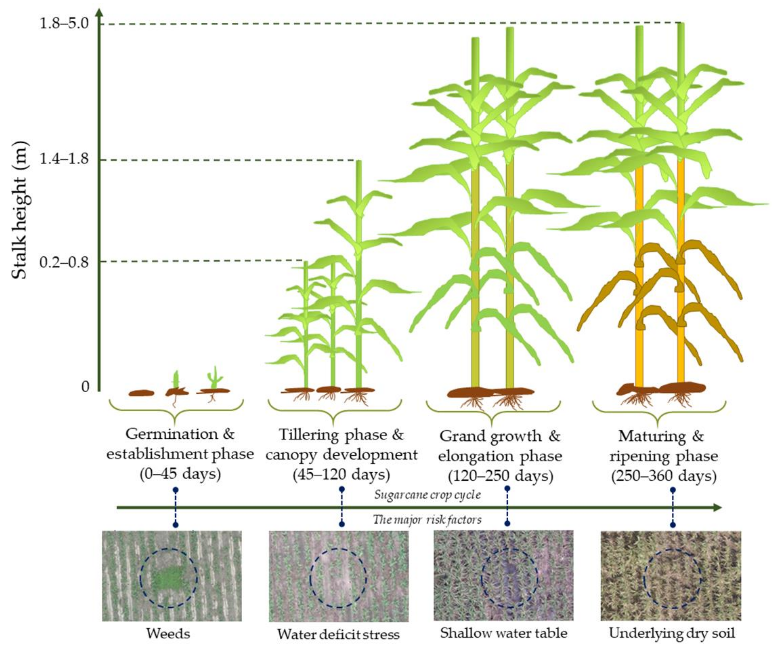
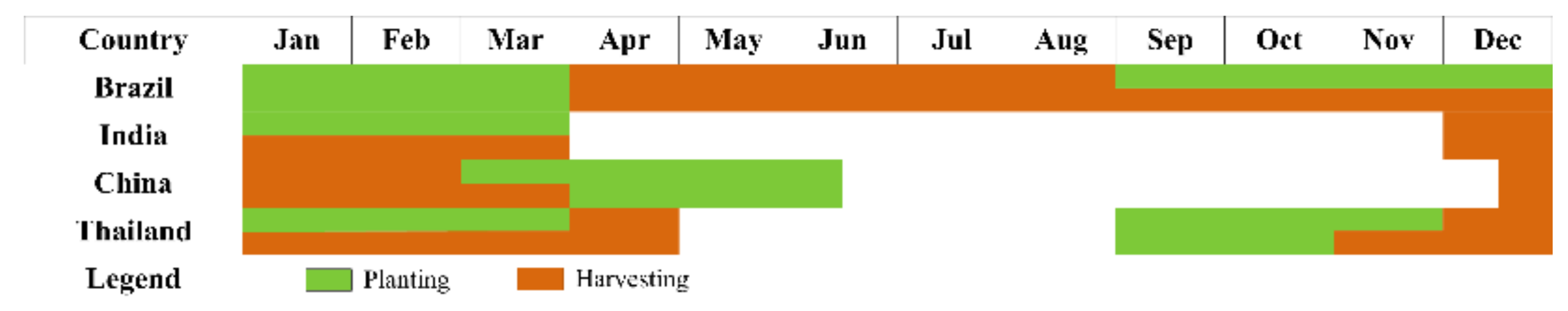
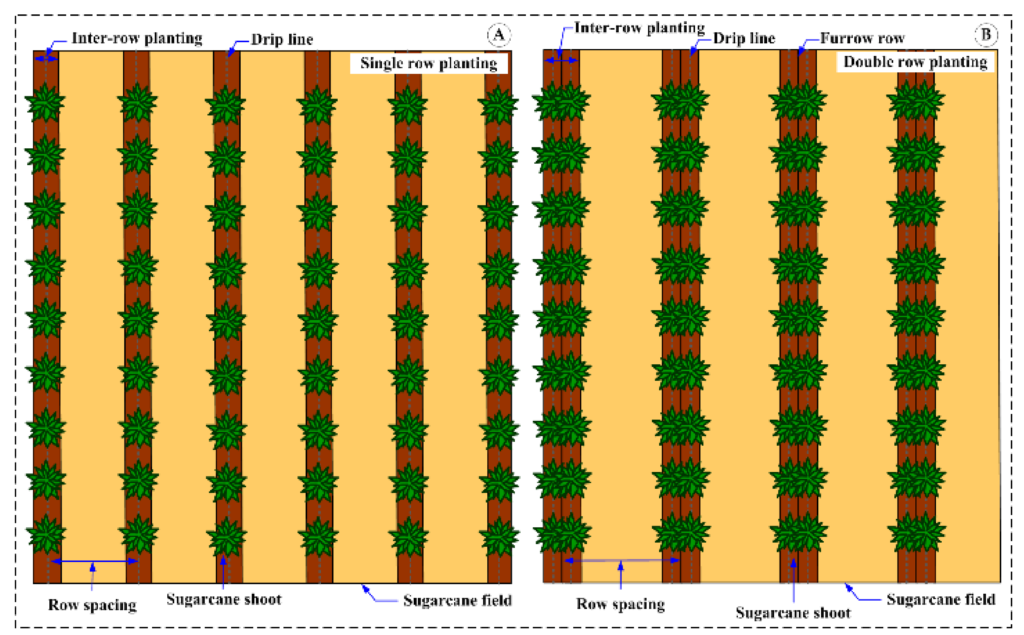
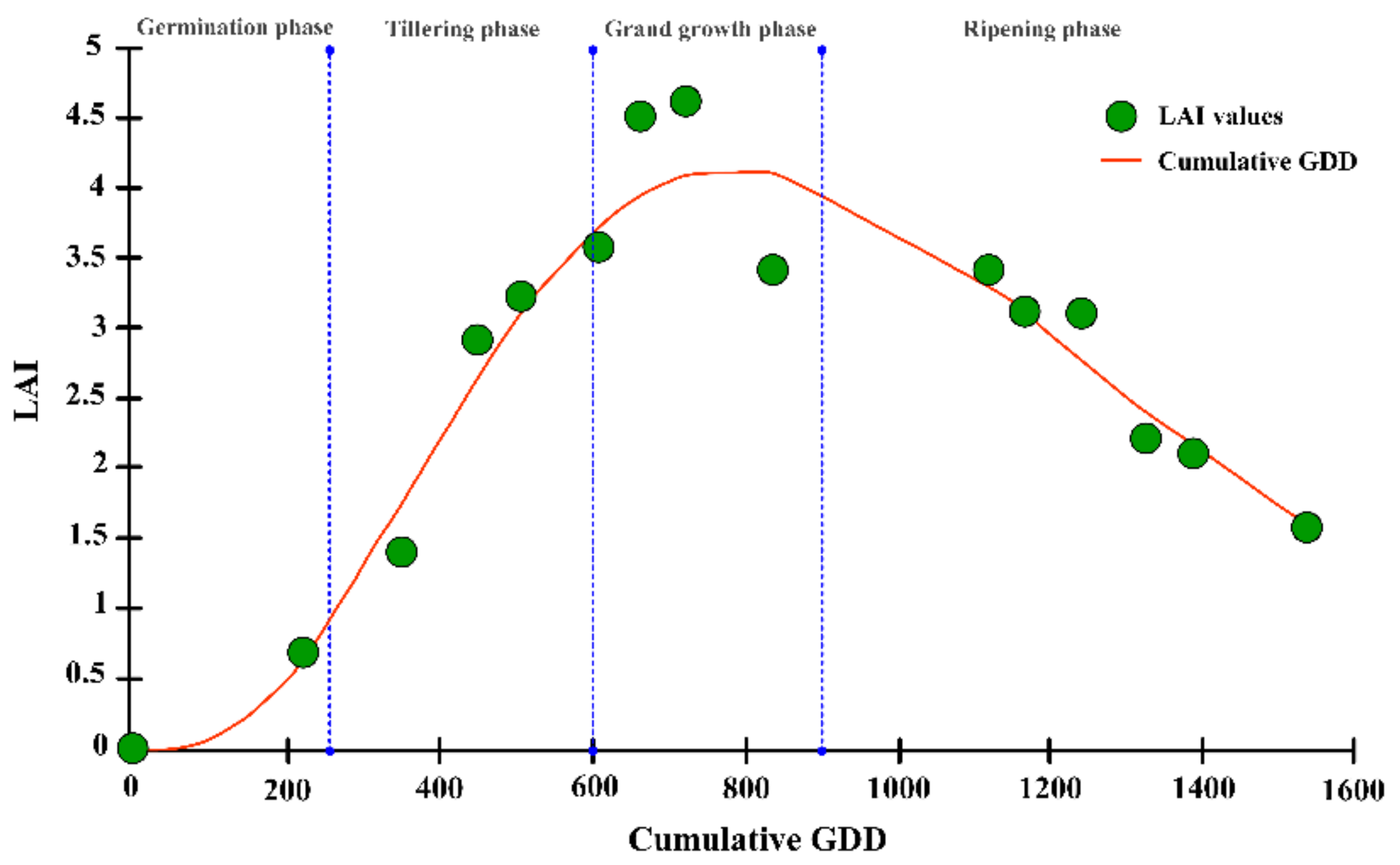
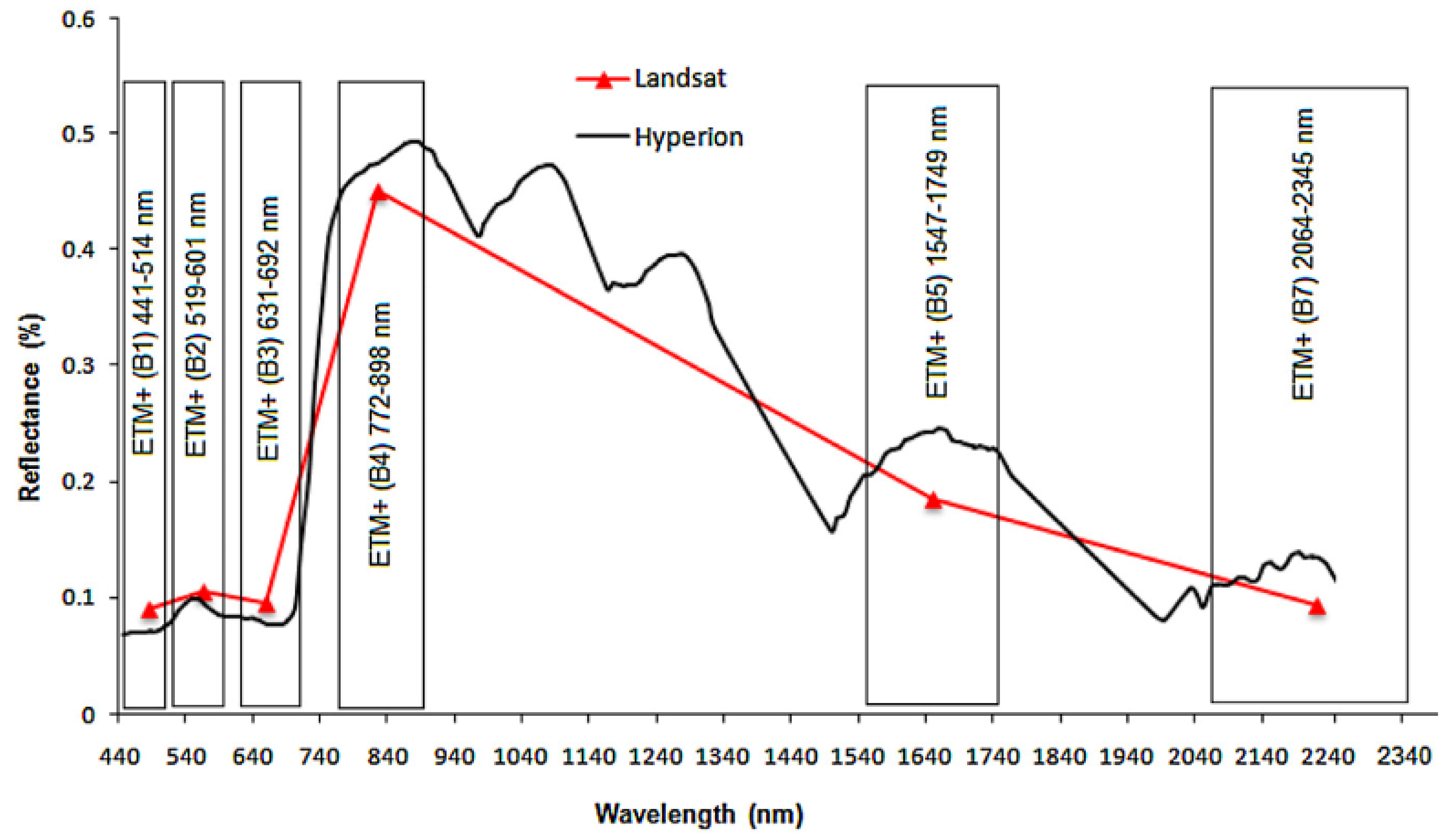
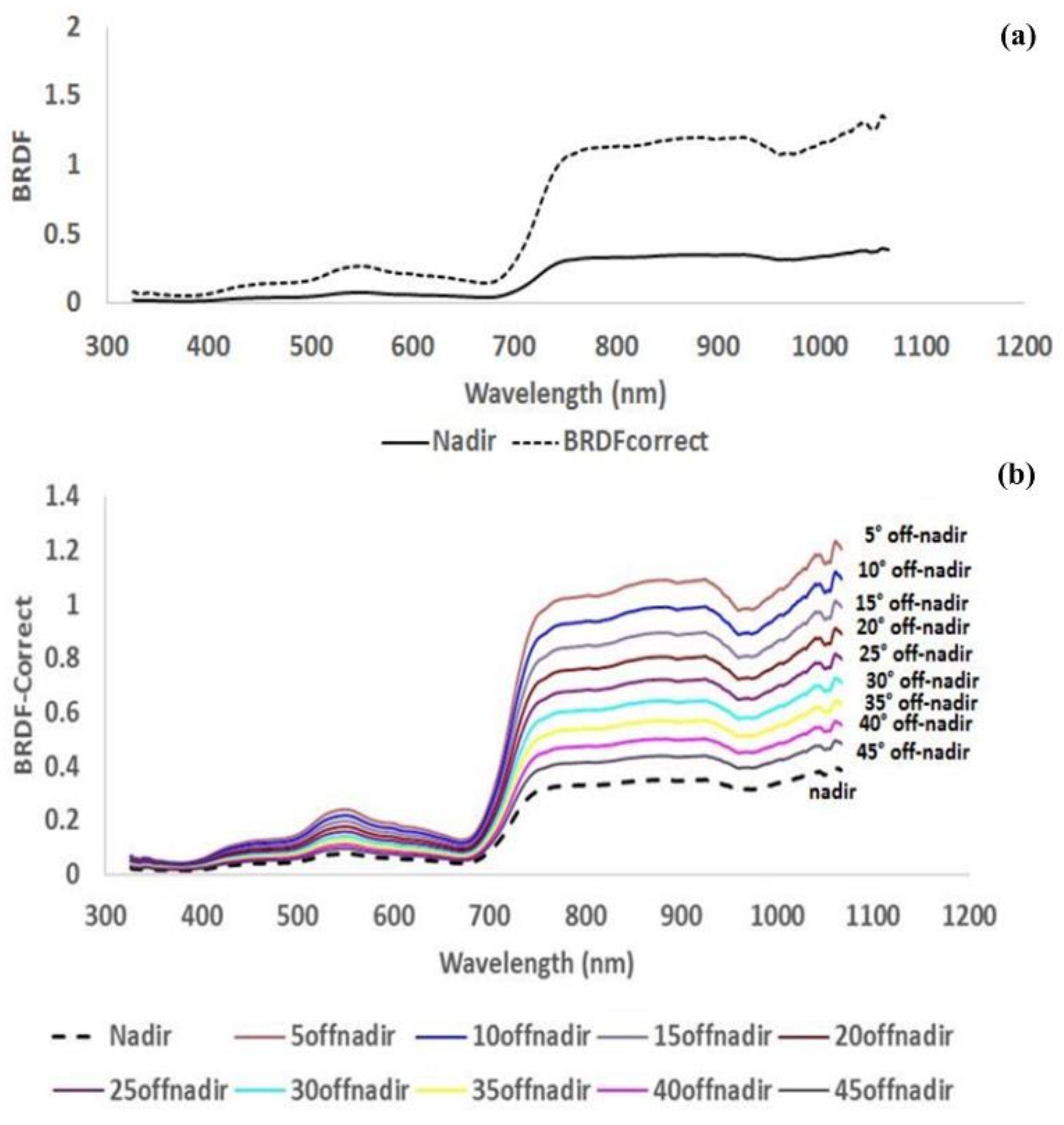
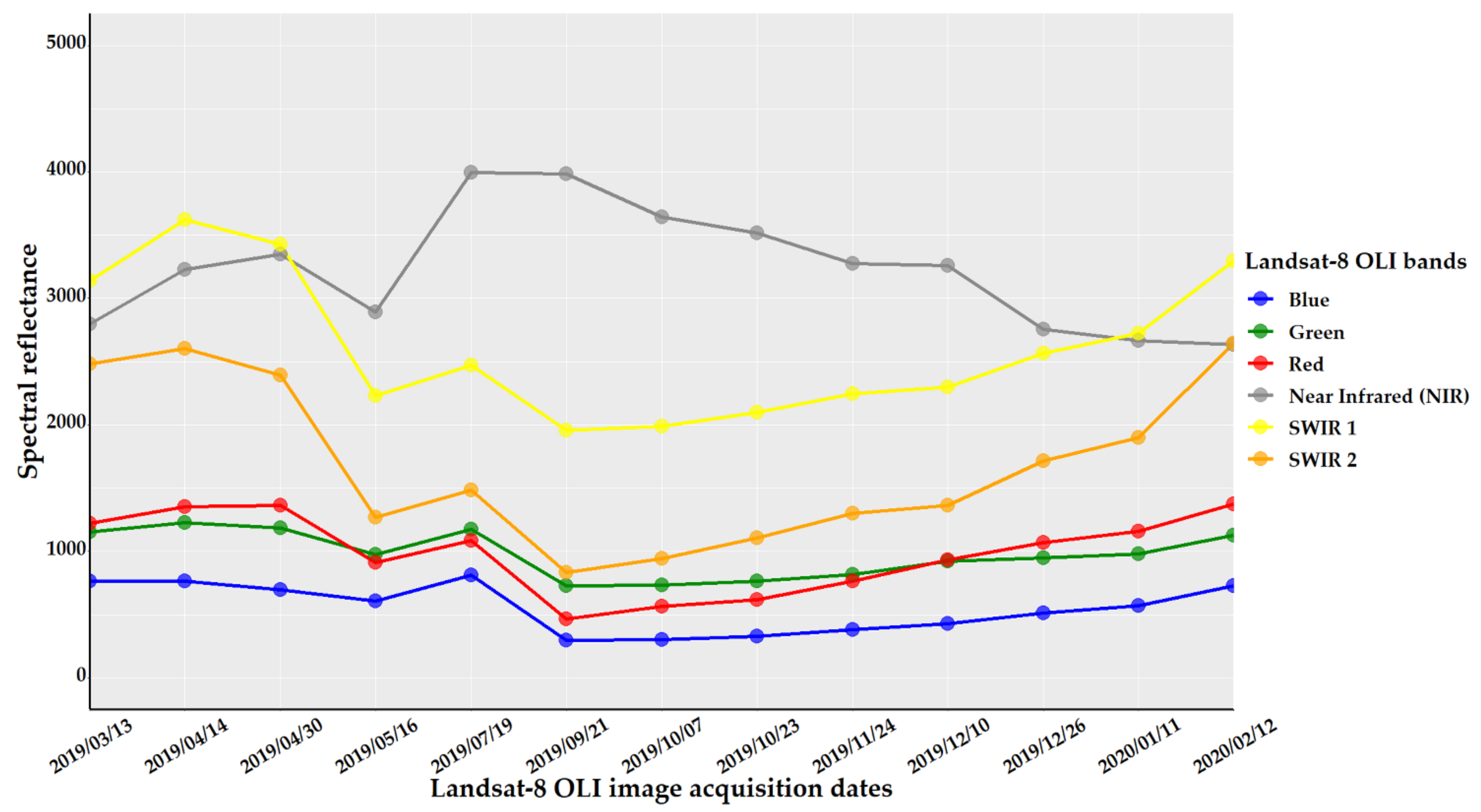
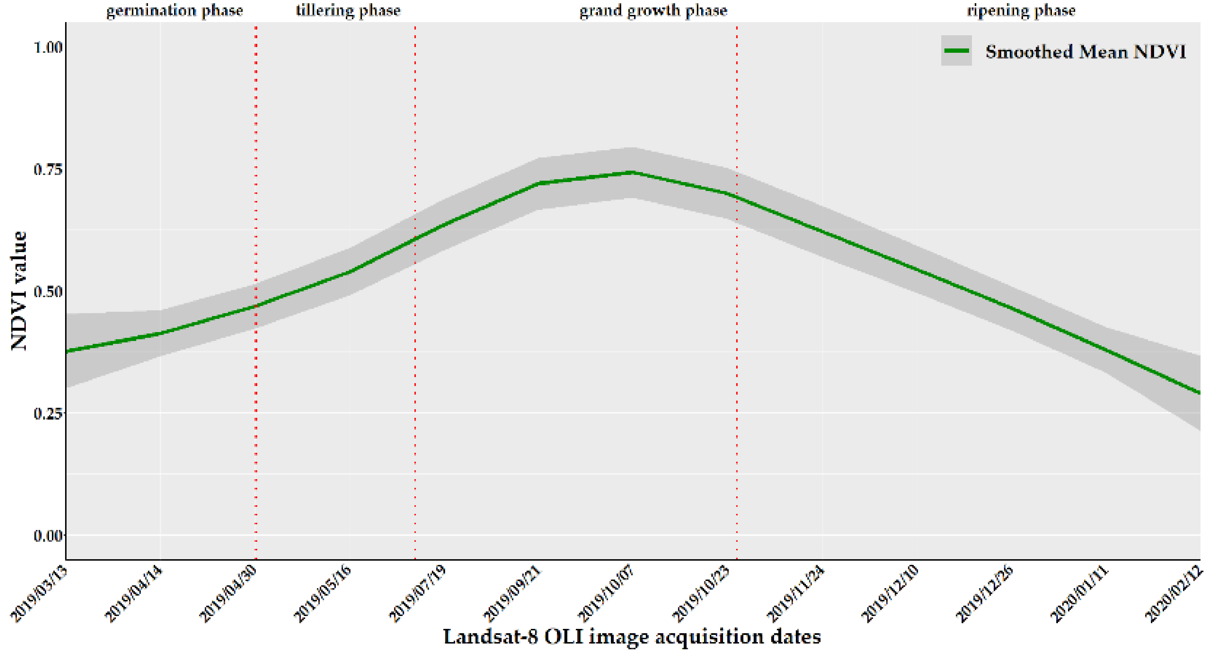
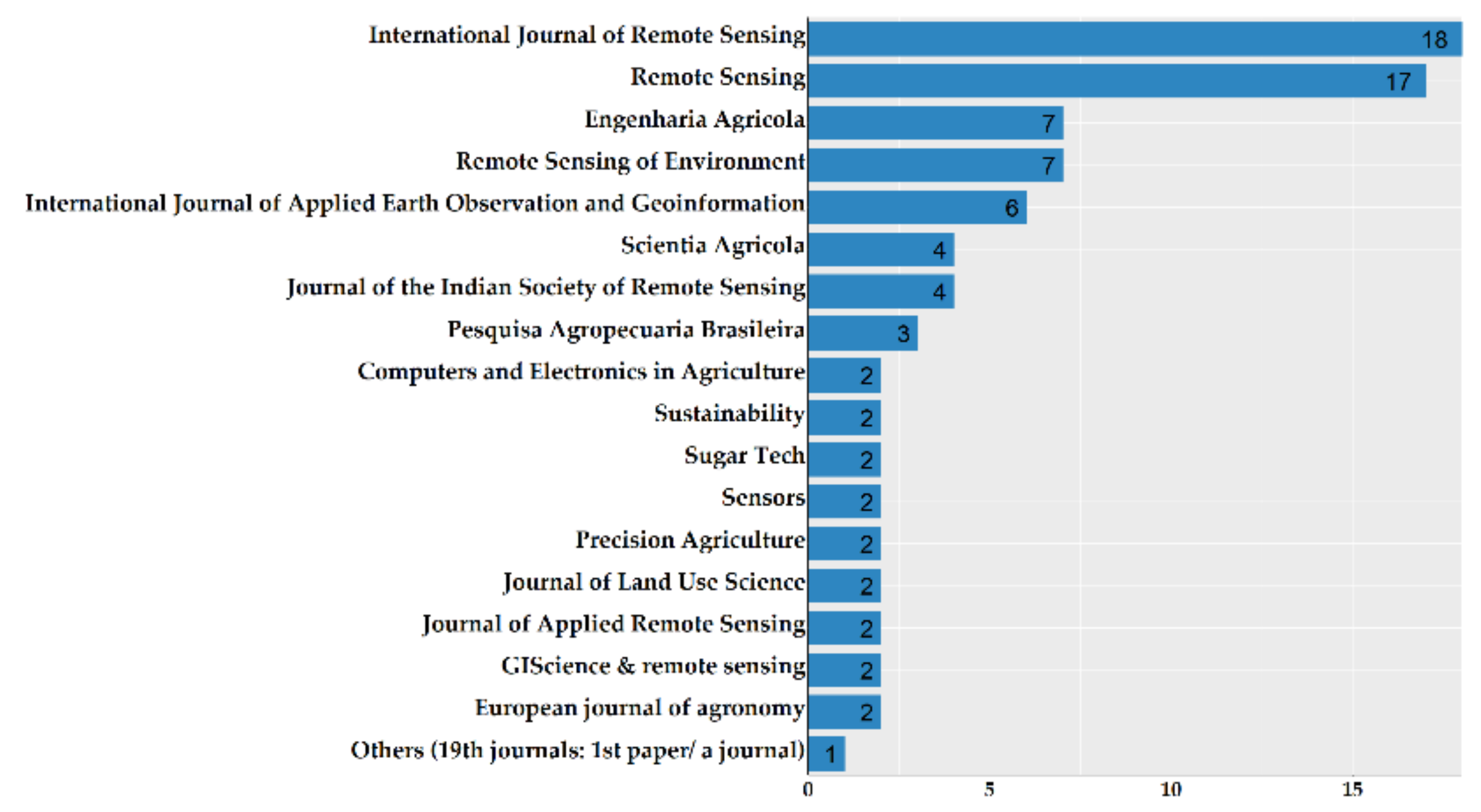
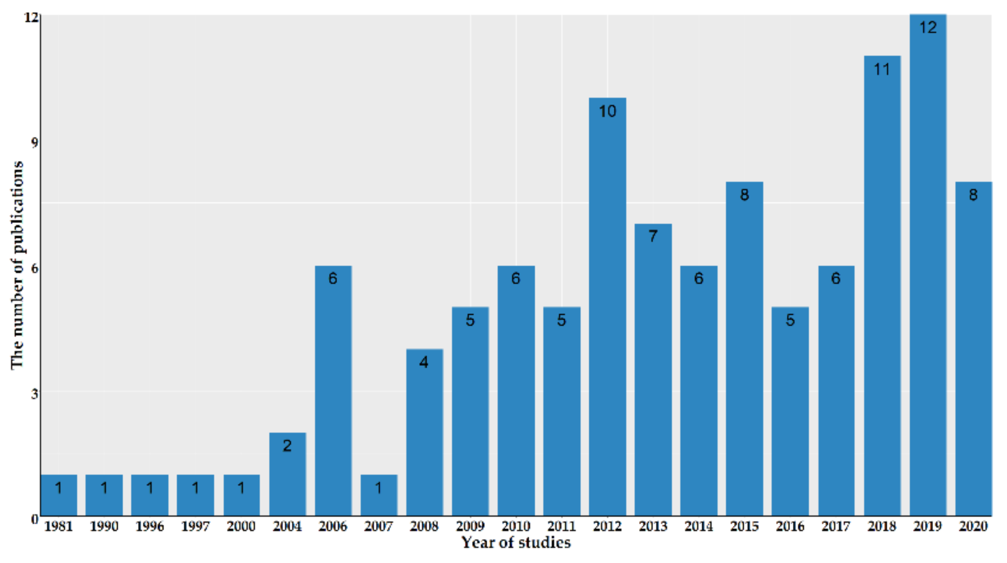
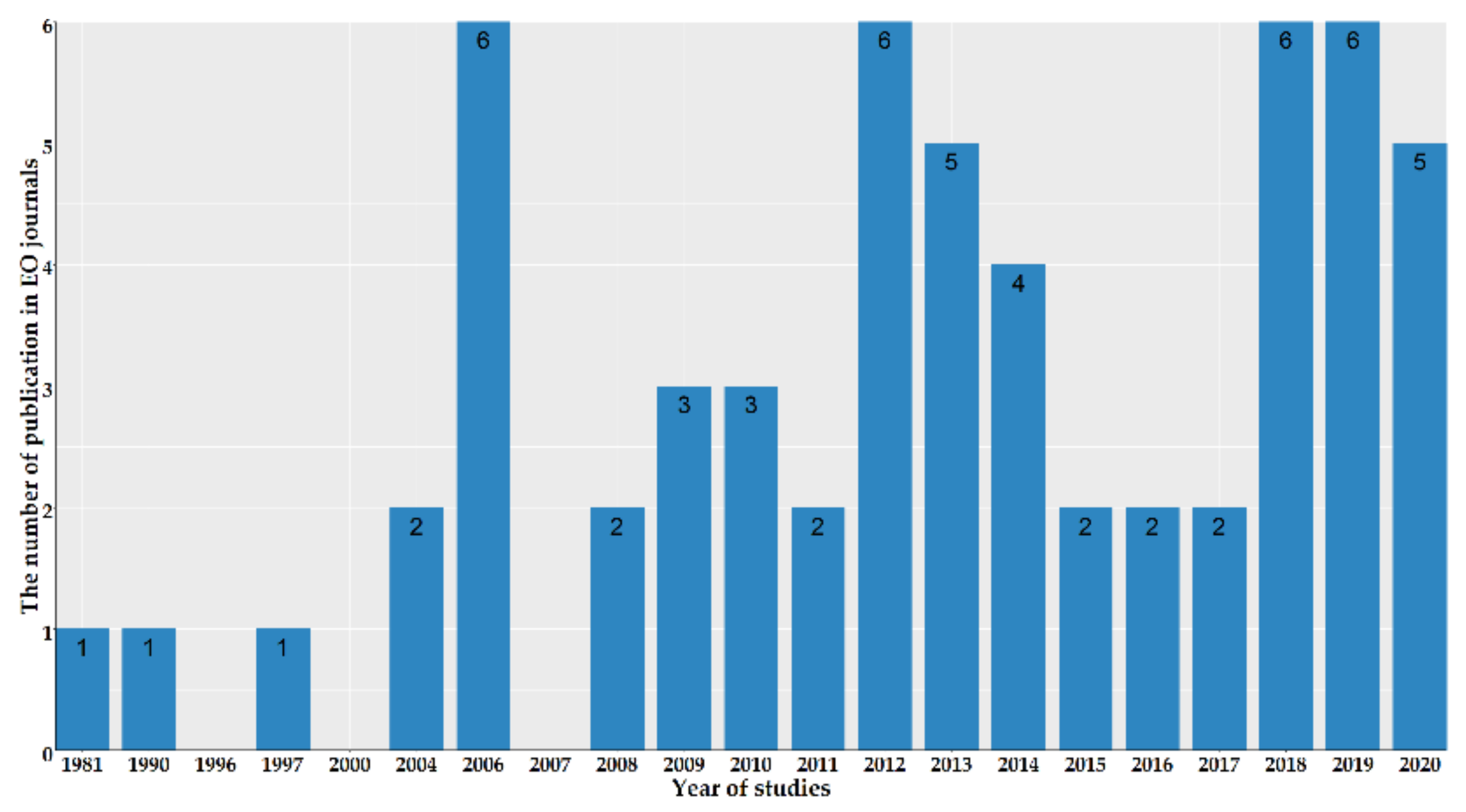
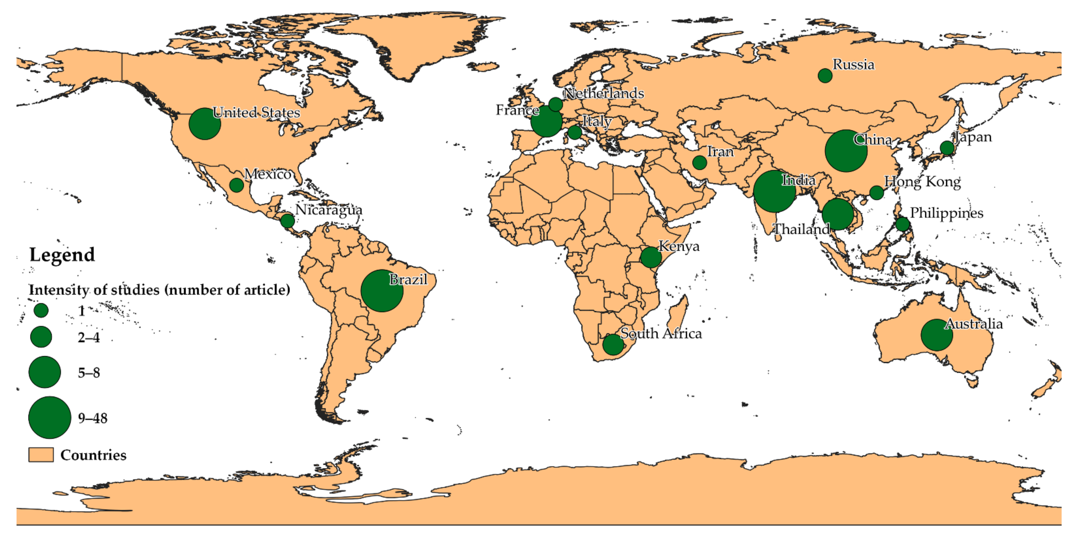
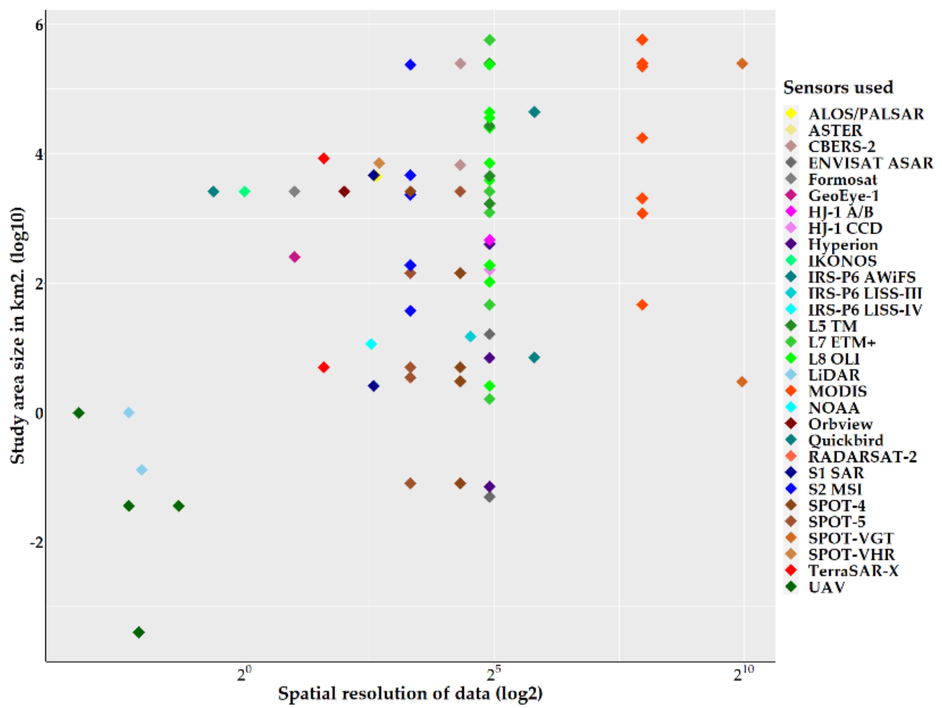
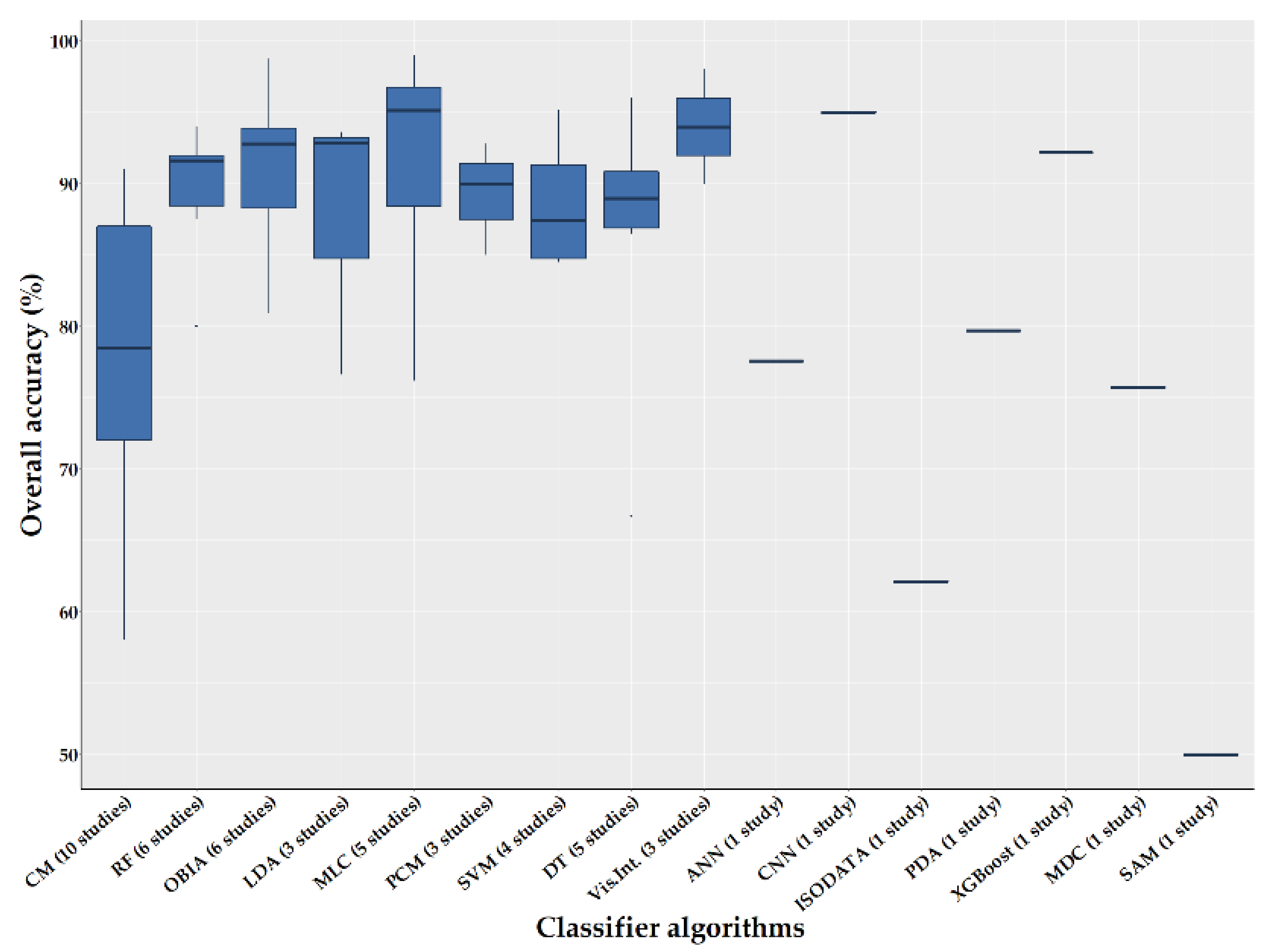
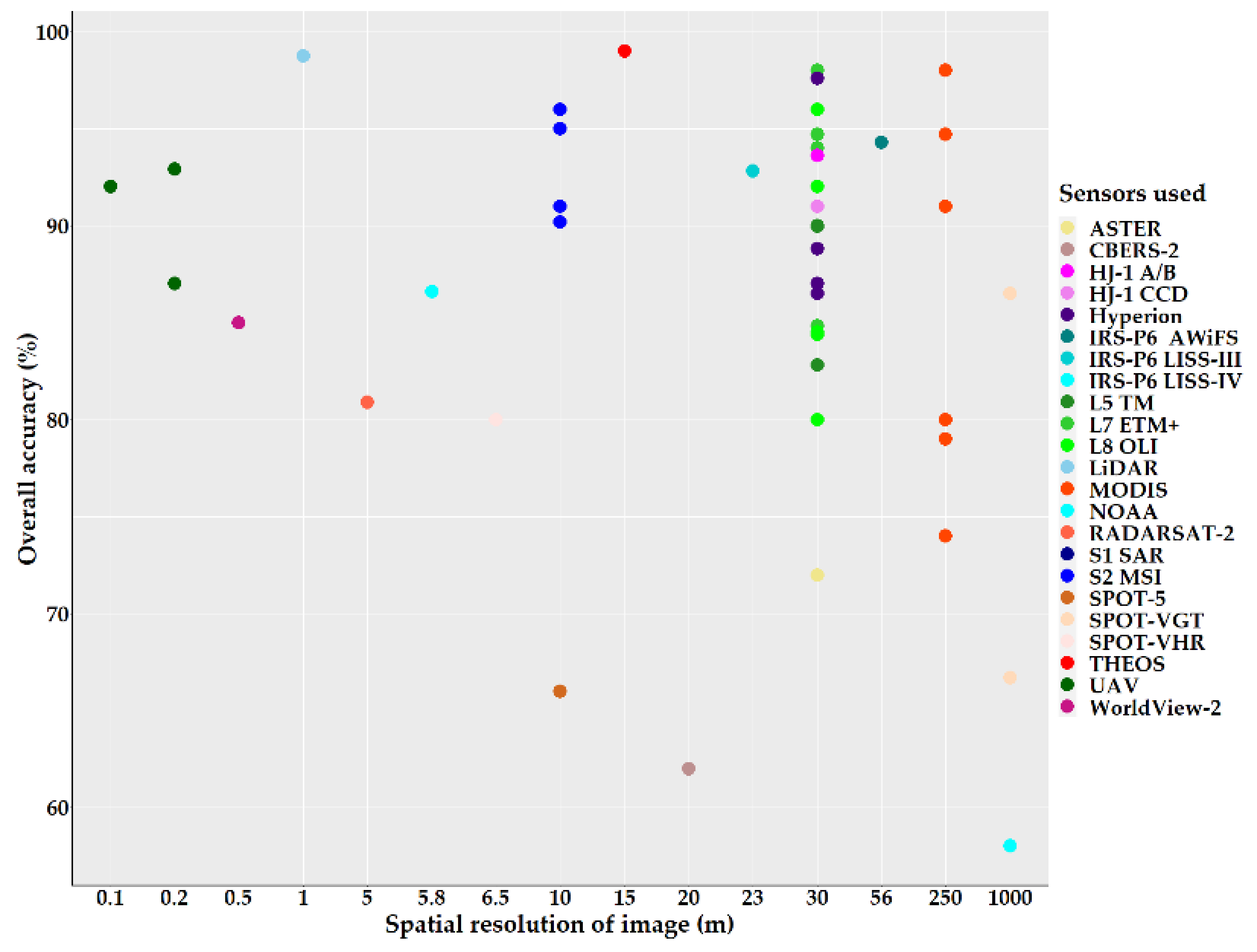
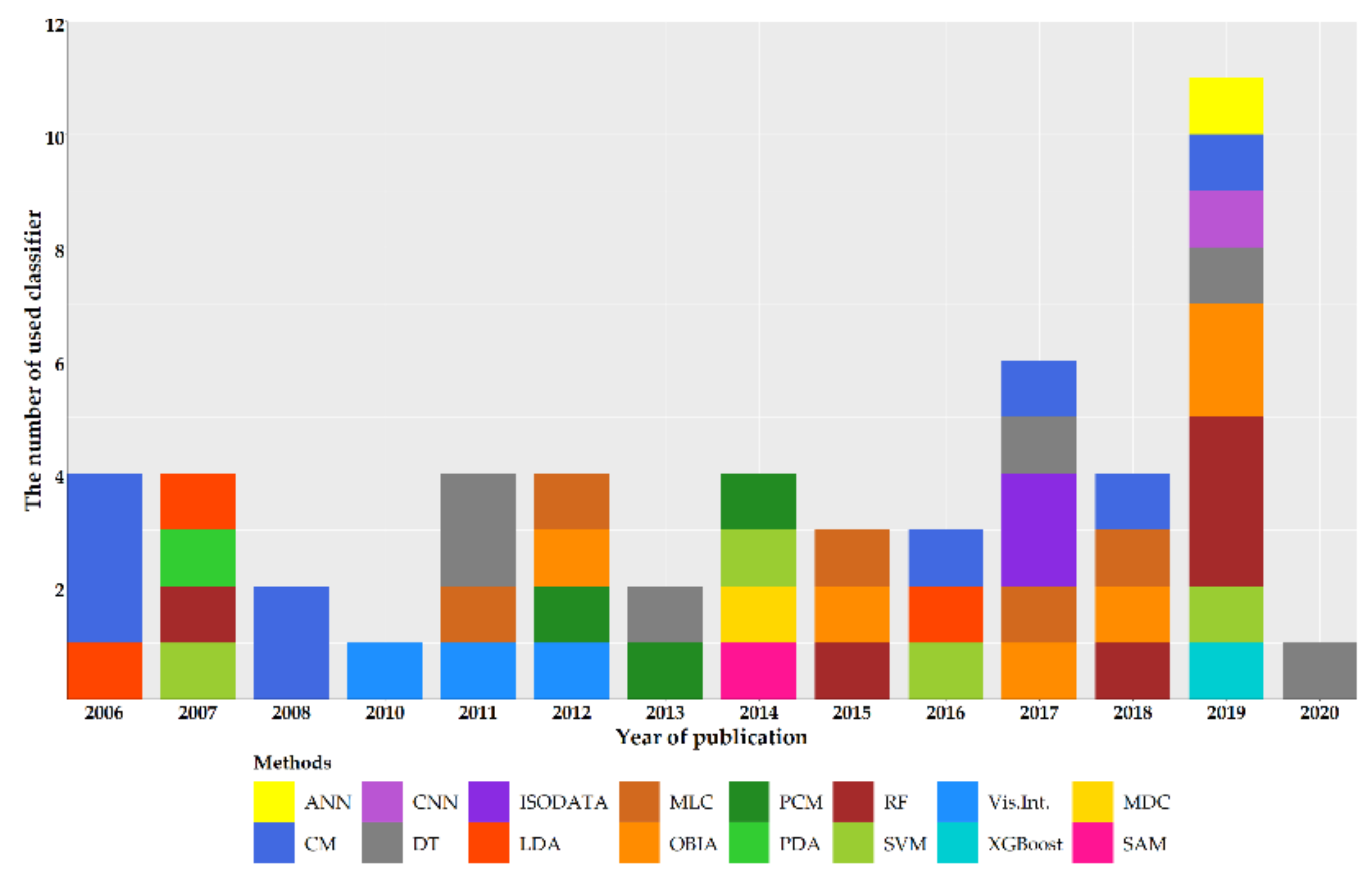
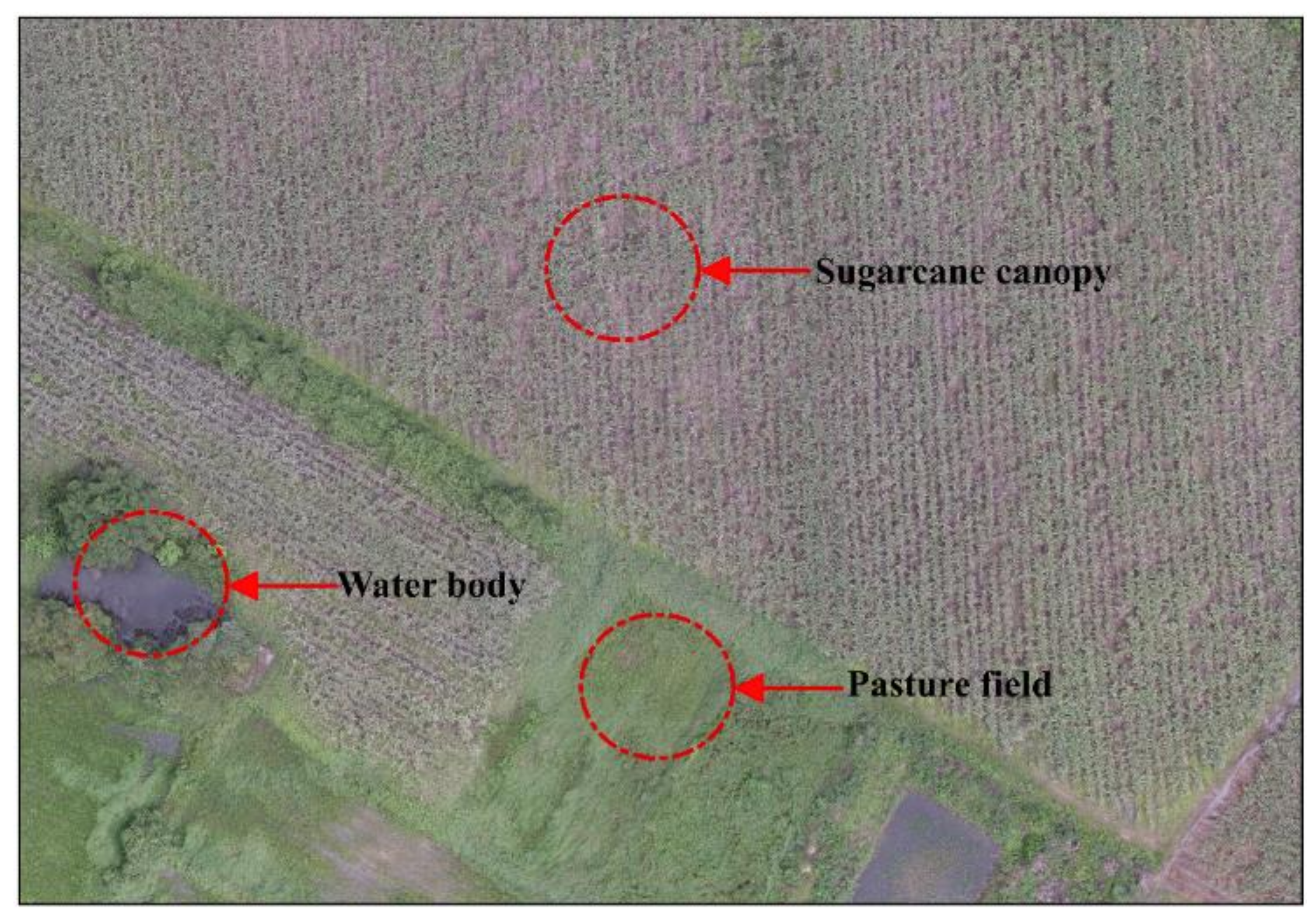
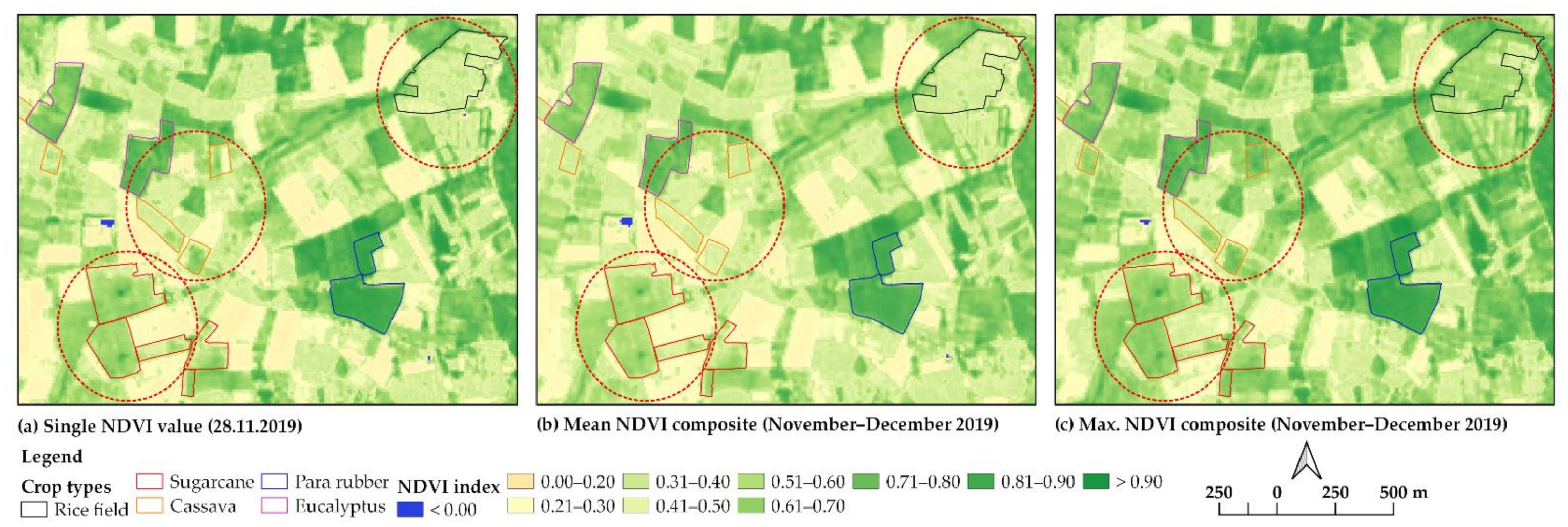
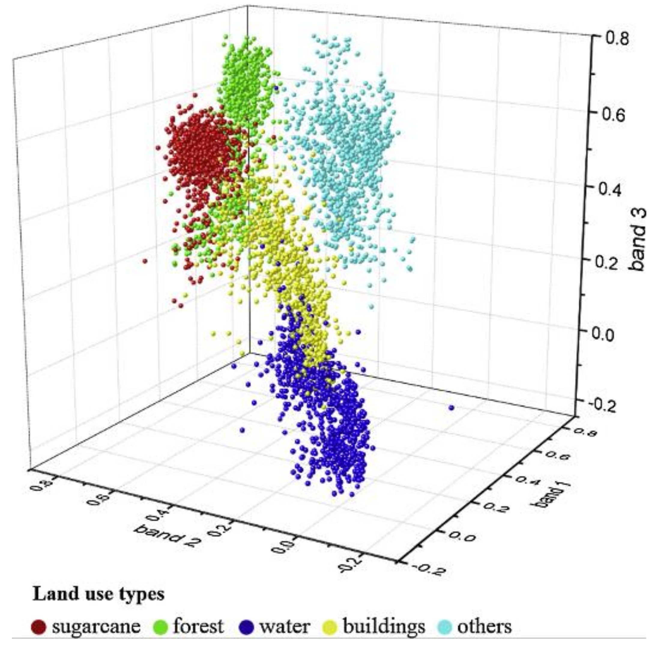
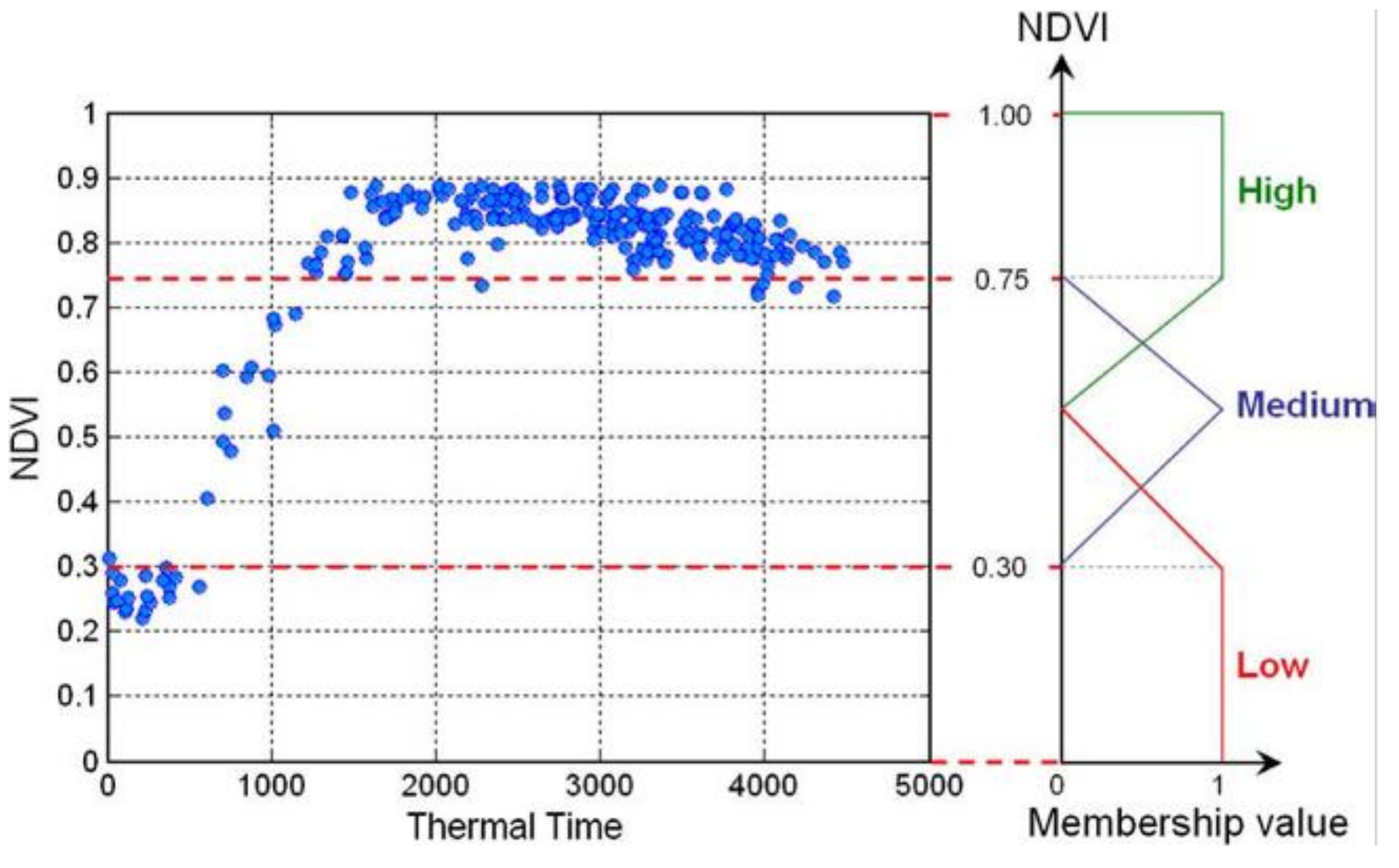
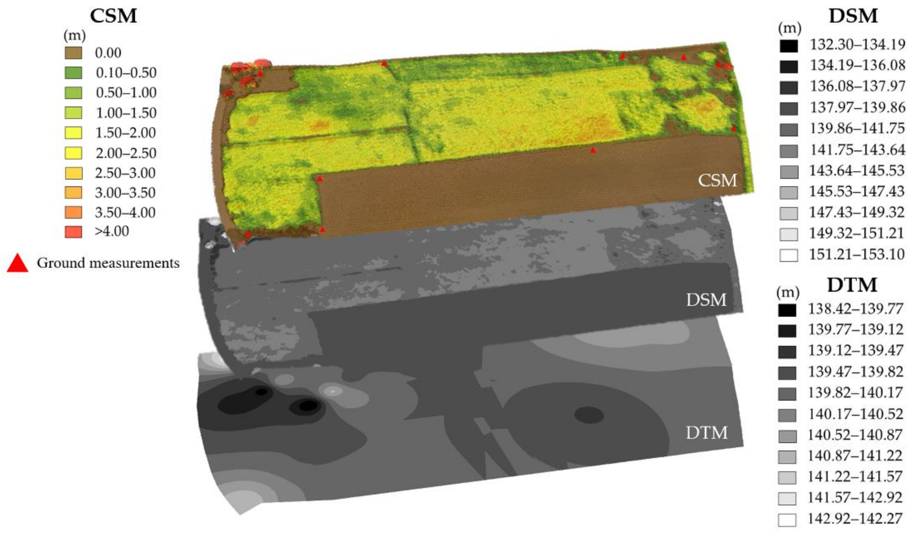
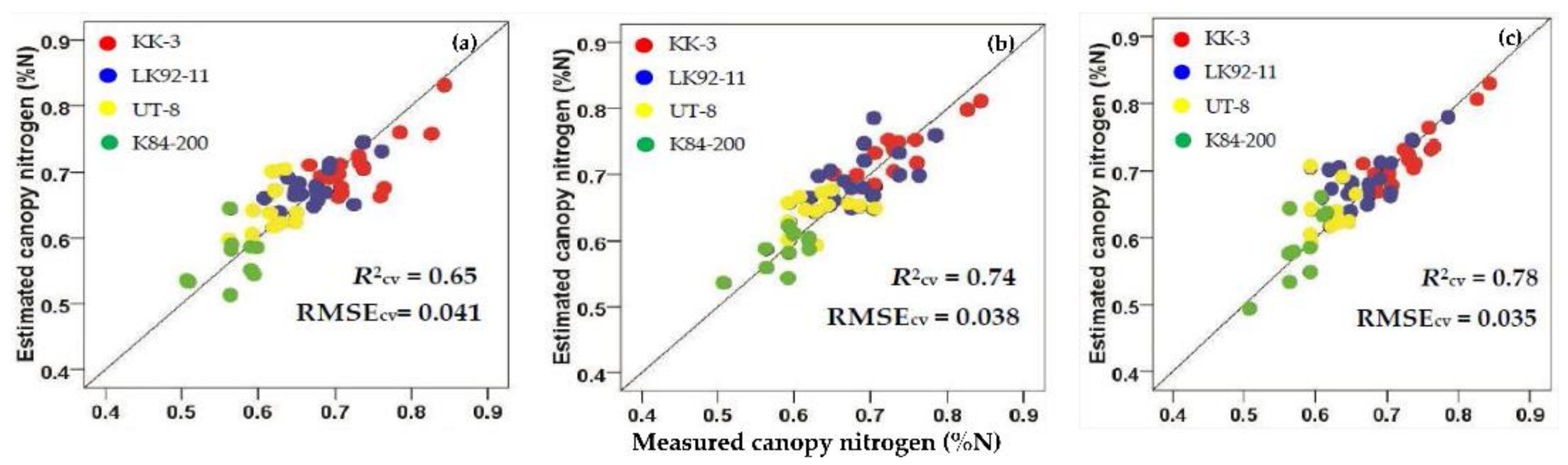
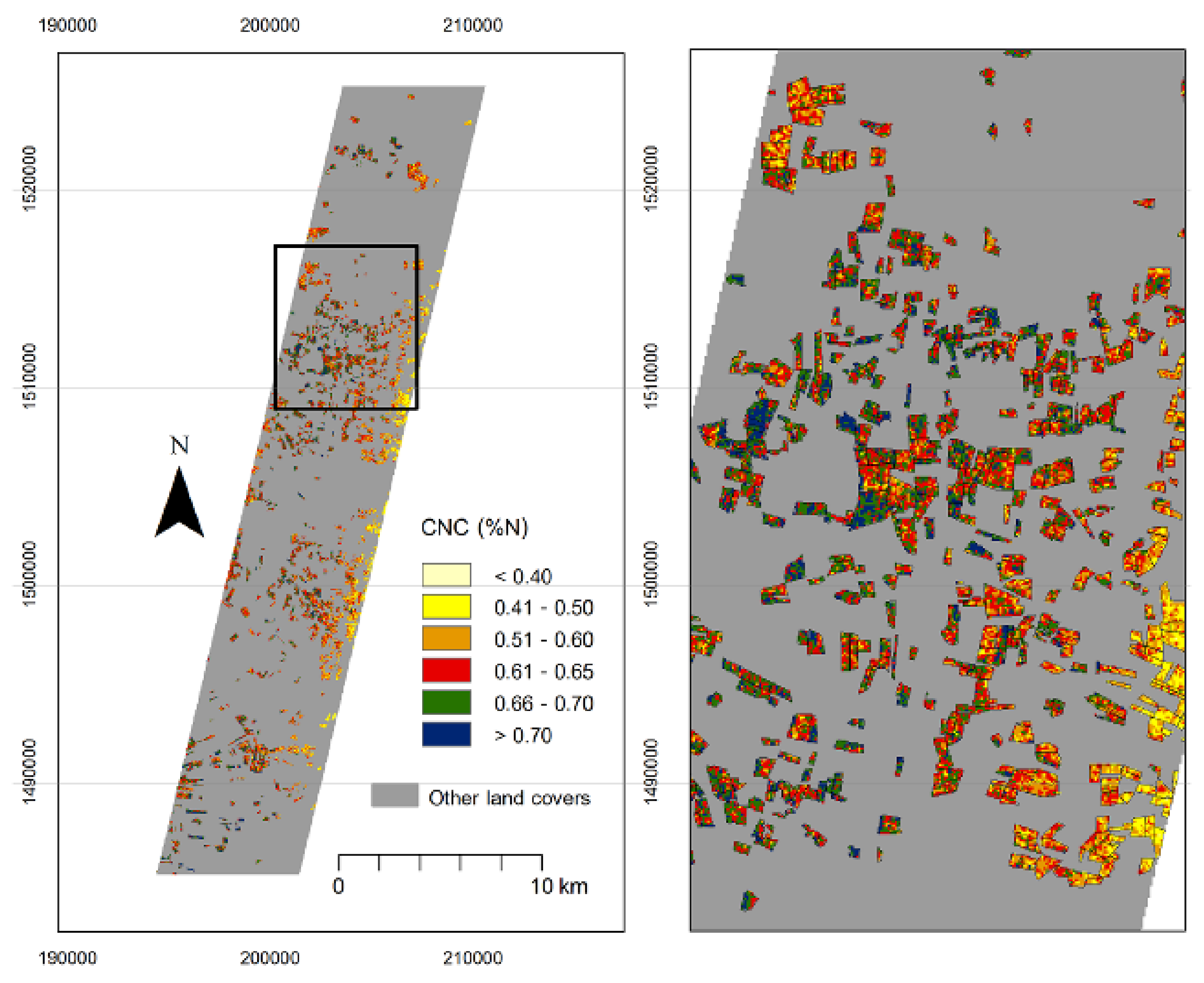
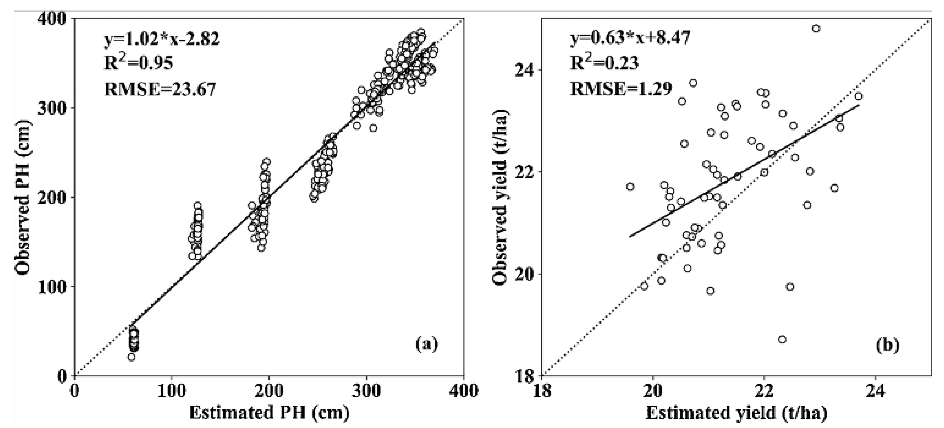
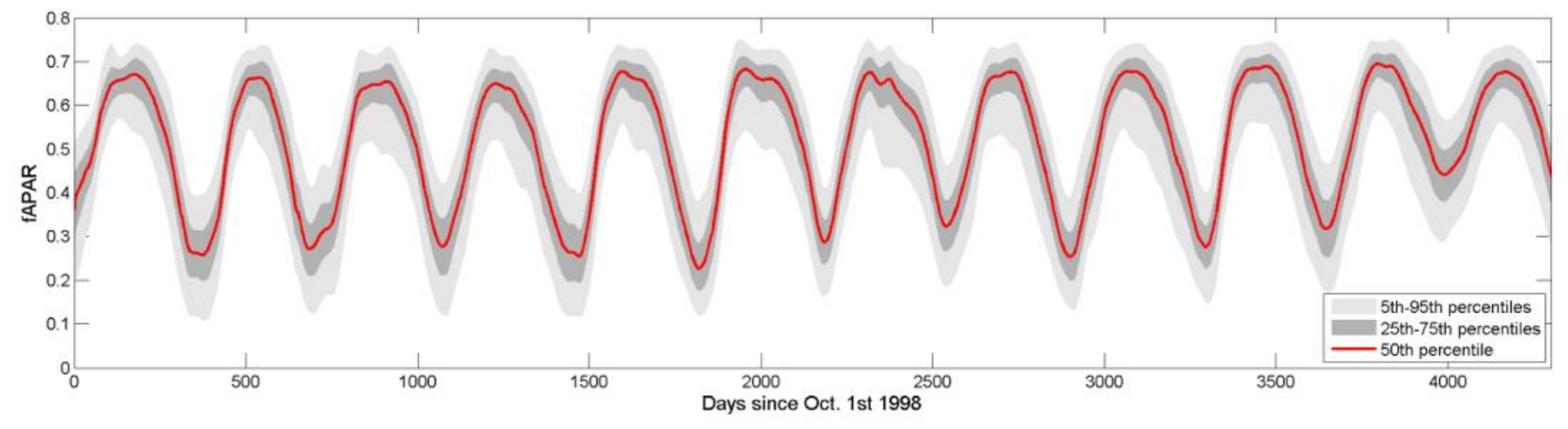
Table 1.
Sugarcane planting information on producing countries.
| Country | Sugarcane Planting Information | References | |||||
|---|---|---|---|---|---|---|---|
| Inter-Row Spacing (m) | Row Spacing (m) | Seeding Density (Setts ha−1) | |||||
| Single | Double | Single | Double | Single | Double | ||
| Brazil | 0.20–0.30 | 0.40–0.60 | 1.20–1.40 | 1.50–1.80 | 90,000–150,000 | 170,000–200,000 | [85,86,87,88,89] |
| India | 0.10–0.20 | 0.20–0.40 | 0.90–1.00 | 1.20–1.50 | 37,500–50,000 | 50,000–75,000 | [88,90,91,92,93] |
| China | 0.25–0.40 | 0.45–0.80 | 1.00–1.20 | 1.20–1.50 | 50,000–80,000 | 100,000–150,000 | [81,82] |
| Thailand | 0.10–0.30 | 0.30–0.40 | 1.20–1.30 | 1.40–1.50 | 60,000–75,000 | 80,000–95,000 | [62,94] |
Table 2.
Sensors used for the sugarcane research and different spatial resolution (m).
| Spatial Resolution of Sensor (m) | Sensors Used | Number of Studies | Percentage of Studies (%) |
|---|---|---|---|
| <1 * | Spectrometry and imaging spectrometer, UAV and LiDAR | 21 | 14 |
| <10 | WorldView-2, GeoEye-1, TerraSAR-X, RADARSAT-2, Formosat, IKONOS, Quickbird, Orbview, IRS-P6 LISS-IV, ALOS/PALSAR, and SPOT-VHR | 17 | 11 |
| 10 to 30 | S1 SAR, S2 MSI, SPOT-5, SPOT-4, CBERS-2, THEOS, IRS-P6 LISS-III, Hyperion, L5 TM, L7 ETM+, L8 OLI, ASTER, ENVISAT ASAR, HJ-1 A/B, and HJ-1 CCD | 86 | 58 |
| 31 to 250 | IRS-P6 AWiFS and MODIS | 17 | 12 |
| 251 to 1000 | SPOT-VGT and NOAA | 7 | 5 |
* Including ground surveys.
Table 3.
The detail of sensors used in intervals of five years and frequency studies in percentage.
| Time Intervals (Years) | Sensor Names and Intensive | Percentage |
|---|---|---|
| 1981–1985 | Spectrometry/spectroscopy (1) | 1 |
| 1986–1990 | Spectrometry/spectroscopy (1) | 1 |
| 1991–1995 | - | 0 |
| 1996–2000 | SPOT-VHR (1), L5 TM (2), MODIS (1), CBERS-2 (1), and NOAA (1) | 4 |
| 2001–2005 | Hyperion (1) and L7 ETM+ (1) | 1 |
| 2006–2010 | Spectrometer/spectroscopy (1), TerraSAR-X (1), SPOT-4 (4), SPOT-5 (6), IRS-P6 LISS-III (1), Hyperion (3), L5 TM (3), L7 ETM+ (6), ENVISAT ASAR (2), MODIS (3), CBERS-2 (2), ASTER (2), NOAA (1), Formosat (1), IKONOS (1), Quickbird (1), Orbview (1), and IRS-P6 AWiFS (1) | 27 |
| 2011–2015 | Spectrometry/spectroscopy (4), WorldView-2 (1), TerraSAR-X (1), ALOS/PALSAR (2), SPOT-4 (2), SPOT-VHR (1), IRS-P6 LISS-III (1), Hyperion (1), L5 TM (10), L7 ETM+ (4), L8 OLI (3), HJ-1 A/B (1), MODIS (4), SPOT-VGT (4), NOAA (1), IRS-P6 AWiFS (1), and THEOS (1) | 28 |
| 2016–2020 | Spectrometry/spectroscopy (8), UAV (10), LiDAR (2), WorldView-2 (1), GeoEye-1 (1), RADARSAT-2 (1), IRS-P6 LISS-IV (2), S1 SAR (4), S2 MSI (6), Hyperion (2), L5 TM (4), L7 ETM+ (4), L8 OLI (7), HJ-1 CCD (1), MODIS (7), and Hyperspectral sensor (1) | 38 |
Table 4.
Summary of different classifier methods, sensors use, and pros and cons for sugarcane mapping.
Table 4.
Summary of different classifier methods, sensors use, and pros and cons for sugarcane mapping.
| Classifier Approaches | Sensors Use | Pros | Cons | Publication |
|---|---|---|---|---|
| CM | HJ-1 CCD, Hyperion, MODIS, and NOAA |
|
| [130,145,165,166,167,168] |
| RF | S1 SAR, S2 MSI, L5 TM, L7 ETM+, L8 OLI, SPOT-VHR, and Hyperion |
|
| [34,43,49,117,169] |
| OBIA | UAV, LiDAR, HJ-1 A/B, L5 TM, L7 ETM+, and RADARSAT-2 |
|
| [3,58,73,74,106,170] |
| LDA | UAV, Hyperion, and L7 ETM+ |
|
| [7,117,141] |
| MLC | THEOS, L5 TM, L8 OLI, LISS-IV, and IRS (AWiFS) |
|
| [162,163,171,172,173] |
| PCM | WorldView-2, LISS-III, and ALOS/PALSAR |
|
| [174,175,176] |
| SVM | S2 MSI, Hyperion, L7 ETM+, and L8 OLI |
|
| [35,45,117,177] |
| DT | S1 SAR, S2 MSI, L5 TM, L7 ETM+, L8 OLI, and LISS-IV |
|
| [155,172,178] |
| Vis.Int. | MODIS, L5 TM, and L7 ETM+ |
|
| [56,179,180] |
| ANN | S2 MSI |
|
| [35] |
| CNN | S2 MSI |
|
| [181] |
| ISODATA | LISS-IV |
|
| [172] |
| PDA | Hyperion |
|
| [117] |
| XGBoost | S1 SAR and S2 MSI |
|
| [43] |
| MDC | Hyperion |
|
| [45] |
| SAM | Hyperion |
|
| [45] |
CM = crop masking, RF = random forest, OBIA = object-based image analysis, LDA = linear discriminant analysis, MLC = maximum likelihood classification, PCM = possibilistic c-mean, SVM = support vector machine, DT = decision tree, Vis.Int. = visual interpretation, ANN = artificial neural network, CNN = convolutional neural network, PDA = penalized discriminant analysis, MDC = minimum distance classification, SAM = spectral angle mapper.
Table 5.
Summary of the number of studies, different methods, data used, and pros and cons for growth anomaly monitoring.
Table 5.
Summary of the number of studies, different methods, data used, and pros and cons for growth anomaly monitoring.
| Number of Studies | Methods | Sensors Use | Pros and Cons | Publication |
|---|---|---|---|---|
| 4 |
| Image time series
|
| [72,219,220,221] |
| 3 |
|
|
| [222,223,224] |
| 3 |
|
|
| [42,89,225] |
| 1 |
|
|
| [226] |
Table 6.
Conclusion of previous studies, the methods, sensor data used, mean RMSE accuracy, and pros and cons for sugarcane yield estimation.
Table 6.
Conclusion of previous studies, the methods, sensor data used, mean RMSE accuracy, and pros and cons for sugarcane yield estimation.
| Number of Studies | Methods | Sensors Use | Mean RMSE Accuracy (t/ha) | Pros and Cons | Publication |
|---|---|---|---|---|---|
| 12 |
| Spectrometry Image time series
| 7.36 |
| [115,124,132,146,148,159,160,161,238,239,240,241] |
| 7 |
| Spectrometry Multi-temporal images
| 12.98 |
| [44,97,149,186,230,242,243] |
| 6 |
|
| 1.29 |
| [3,46,47,84,244,245] |
| 4 |
| A single image data
| NA |
| [105,246,247,248] |
| 1 |
| Image time series
| 8.2 |
| [249] |
RMSE = root mean square error, VI = vegetation indices, NA = no appears mean accuracy of RMSE.
Publisher’s Note: MDPI stays neutral with regard to jurisdictional claims in published maps and institutional affiliations. |
© 2021 by the authors. Licensee MDPI, Basel, Switzerland. This article is an open access article distributed under the terms and conditions of the Creative Commons Attribution (CC BY) license (https://creativecommons.org/licenses/by/4.0/).
Share and Cite
MDPI and ACS Style
Som-ard, J.; Atzberger, C.; Izquierdo-Verdiguier, E.; Vuolo, F.; Immitzer, M. Remote Sensing Applications in Sugarcane Cultivation: A Review. Remote Sens. 2021, 13, 4040. https://0-doi-org.brum.beds.ac.uk/10.3390/rs13204040
AMA Style
Som-ard J, Atzberger C, Izquierdo-Verdiguier E, Vuolo F, Immitzer M. Remote Sensing Applications in Sugarcane Cultivation: A Review. Remote Sensing. 2021; 13(20):4040. https://0-doi-org.brum.beds.ac.uk/10.3390/rs13204040
Chicago/Turabian StyleSom-ard, Jaturong, Clement Atzberger, Emma Izquierdo-Verdiguier, Francesco Vuolo, and Markus Immitzer. 2021. "Remote Sensing Applications in Sugarcane Cultivation: A Review" Remote Sensing 13, no. 20: 4040. https://0-doi-org.brum.beds.ac.uk/10.3390/rs13204040
Note that from the first issue of 2016, this journal uses article numbers instead of page numbers. See further details here.