
Adversarial Self-Supervised Learning for Robust SAR Target Recognition

1
State Key Laboratory of Complex Electromagnetic Environment Effects on Electronics and Information System, National University of Defense Technology, Changsha 410073, China
2
Beijing Institute of Remote Sensing Information, Beijing 100092, China
*
Author to whom correspondence should be addressed.
Remote Sens. 2021, 13(20), 4158; https://0-doi-org.brum.beds.ac.uk/10.3390/rs13204158
Submission received: 23 August 2021
/
Revised: 30 September 2021
/
Accepted: 15 October 2021
/
Published: 17 October 2021
(This article belongs to the Special Issue Target Detection and Information Extraction in Radar Images)
Abstract
:Synthetic aperture radar (SAR) can perform observations at all times and has been widely used in the military field. Deep neural network (DNN)-based SAR target recognition models have achieved great success in recent years. Yet, the adversarial robustness of these models has received far less academic attention in the remote sensing community. In this article, we first present a comprehensive adversarial robustness evaluation framework for DNN-based SAR target recognition. Both data-oriented metrics and model-oriented metrics have been used to fully assess the recognition performance under adversarial scenarios. Adversarial training is currently one of the most successful methods to improve the adversarial robustness of DNN models. However, it requires class labels to generate adversarial attacks and suffers significant accuracy dropping on testing data. To address these problems, we introduced adversarial self-supervised learning into SAR target recognition for the first time and proposed a novel unsupervised adversarial contrastive learning-based defense method. Specifically, we utilize a contrastive learning framework to train a robust DNN with unlabeled data, which aims to maximize the similarity of representations between a random augmentation of a SAR image and its unsupervised adversarial example. Extensive experiments on two SAR image datasets demonstrate that defenses based on adversarial self-supervised learning can obtain comparable robust accuracy over state-of-the-art supervised adversarial learning methods.
1. Introduction
Synthetic aperture radar (SAR) actively emits microwaves and improves azimuth resolution through the principle of a synthetic aperture to obtain large-area high-resolution radar images [1]. SAR images have been widely used for automatic target detection and recognition in both civil and military applications. Due to their imaging mechanism, different terrains in SAR images exhibit several special phenomena such as overlap, shadows, and perspective shrinkage. Moreover, coherent speckle noises are apparent in SAR images. It is difficult to manually design effective features for SAR target recognition [2]. With the rapid development of deep learning technology, deep neural network (DNN) models have been widely used for SAR target recognition. Shao et al. [3] analyzed the performance of different DNNs on the MSTAR [4] dataset according to classification accuracy, training time, and some other metrics to verify the superiority of DNNs for SAR target recognition. Ding et al. [5] carried out angle synthesis of the training data for DNN-based recognition models. Ayzel et al. [6] proposed all convolutional neural networks (A-ConvNet), which do not contain a fully connected layer. Gu and Xu [7] proposed that a wider convolution kernel was more suitable for a SAR image with stronger speckles noise, taking the multi-scale feature extraction module as the bottom layer of the network.
Despite the great success that DNN models have obtained, they have proved to be very sensitive to adversarial examples: inputs that are specifically designed to cause the target model to produce erroneous outputs [8]. The vulnerability of DNN models to imperceptibly small perturbations raises security concerns from a number of safety-sensitive applications [9]. Szegedy et al. [8] first discovered that DNNs were very susceptible to adversarial examples using a box-constrained L-BFGS algorithm. Goodfellow et al. [10] noted that the linear nature of DNN is the primary cause for its vulnerability to adversarial perturbations. Based on this theory, they proposed a gradient-based approach to generate adversarial examples, named the fast gradient sign method (FGSM). Moosavi-Dezfooli et al. [11] proposed the DeepFool algorithm to simplify L-BFGS and fool deep models, and thus reliably quantified the robustness of models. Kurakin et al. [12] proposed to incorporate iterative methods to approximate the inner maximization problem. Moosavi-Dezfooli et al. [13] further found that the existence of universal adversarial examples by adding very small perturbation vectors to original images could cause error outputs for different DNNs with high probability. Although these adversarial examples may remain imperceptible to a human observer, they can easily fool the DNN models to yield the wrong predictions [9].
So far, there are only a handful of studies [14,15] that explore the threat of adversarial attacks on DNNs for SAR target recognition. Deep SAR target recognition models are more likely to suffer from the overfitting problem, resulting in a weaker generalization capability and greater sensitivity to perturbation [14]. Hence, their vulnerability to adversarial attacks might be even more serious. An example of adversarial attacks on DNN models for SAR target recognition is shown in Figure 1. It can be observed that, although the difference between the adversarial examples and the original ones is too small to be perceived by human vision, it can fool the DNN model. This phenomenon limits the practical deployment of DNN models in the safety-critical SAR target recognition field.
Adversarial defense methods can enhance adversarial robustness and further lead to robust SAR target recognition. Among them, adversarial training (AT) and AT-based defenses, which augment training data with adversarial examples perturbed to maximize the loss on the target model, remain a highly effective method for safeguarding DNNs from adversarial examples [9]. Such a strategy requires a large amount of labeled data as support. The labeling and sample efficiency challenges of deep learning, in fact, are further exacerbated by its vulnerability to adversarial attacks. The sample complexity of learning an adversarially robust model with current methods is significantly higher than that of standard learning [16]. Additionally, AT-based techniques have been observed to cause an undesirable decline in standard accuracy (the classification accuracy on unperturbed inputs) while increasing robust accuracy (the classification accuracy on worst-case perturbed inputs) [16,17,18].
Recent research [19] proposed the use of unlabeled data for training adversarially robust DNN models. Self-supervised learning holds great promise for improving representations with unlabeled data and has shown great potential to enhance adversarial robustness. Hendrycks et al. [17] proposed a multi-task learning framework that incorporated a self-supervised objective to be co-optimized with the conventional classification loss. Jiang et al. [18] improved robustness by learning representations that were consistent under both augmented data and adversarial examples. Chen et al. [16] generalized adversarial training to different self-supervised pretraining and fine-tuning schemes. Other studies [18,20,21] exploited contrastive learning to improve model robustness in unsupervised/semi-supervised settings and achieved advanced robustness.
Though a plethora of adversarial defense methods has been proposed, the corresponding evaluation is often inadequate. For example, by evaluating simple white-box attacks, most adversarial defenses pose a false sense of robustness by introducing gradient masking, which can be easily circumvented and defeated [22]. Therefore, rigorous and extensive evaluation of adversarial robustness is necessary for SAR target recognition.
To address the aforementioned issues, in this paper, we systematically analyzed the effect of adversarial attacks and defenses on DNNs and utilized adversarial self-supervised learning to enhance robustness for SAR target recognition. The main contributions of this article are summarized as follows:
- (1)
- We systematically evaluated adversarial attacks and defenses in SAR target recognition tasks using both data-oriented robustness metrics and model-oriented robustness metrics. These metrics provide detailed characteristics of DNN models under adversarial scenarios.
- (2)
- We introduced adversarial self-supervised learning into SAR target recognition tasks for the first time. The defenses based on adversarial self-supervised learning obtained comparable robustness to supervised adversarial learning approaches without using any class labels, while achieving significantly better standard accuracy.
- (3)
- We propose a novel defense method, unsupervised adversarial contrastive learning (UACL), which explicitly suppresses vulnerability in the representation space by maximizing the similarity of representations between clean data and corresponding unsupervised adversarial examples.
The rest of this paper is organized as follows. In Section 2, we describe the adversarial robustness of SAR target recognition. In Section 3, we review the defenses based on adversarial self-supervised learning and propose our method, UACL. In Section 4, we present the information on datasets used in this paper and the experimental results. Our conclusions and other discussions are summarized in Section 5.
2. Adversarial Robustness of SAR Target Recognition
2.1. Definition of Adversarial Robustness
A DNN model for SAR target recognition can be described as a function parameterized by , which maps input to label . Given data distribution D over pairs (), the goal of the learning algorithm is to find that can minimize the expected risk, i.e.,
where is the cross-entropy classification loss between the output of the DNN model and the true labels. In practice, we do not have access to the full data distribution D and only know a subset of training samples . Thus, cannot be obtained by minimizing Equation (1), and it is usually obtained as the solution to the empirical risk minimization problem:
The difference between the expected risk and the empirical risk attained by DNN model is known as the generalization gap. Generally speaking, a DNN model achieves strong robustness when its generalization gap is small [23]. The amount and quality of training datasets are critical to training robust models.
A DNN model can extract image feature, and its entries of the output of the last layer with are generally referred to as logits. To be more interpretable, logits are normally mapped to a set of probabilities using a soft maximum operator, i.e.,
The predicted class is the index of the highest estimated probability.
A notable feature of most DNNs is that, in most cases, the decision boundary appears relatively far from any typical sample. For most DNNs used in SAR target recognition, one needs to add random noise with a very large variance, σ2, to fool a model. Intriguingly, the robustness to random noise contrasts with the extra vulnerability of DNNs to adversarial perturbations [8]. Surprisingly, we can always find adversarial examples for any input, which suggests that some directions for which the decision boundary is very close to the input sample always exist. Adding perturbation in such a direction can fool the model easily.
We can define adversarial perturbation as follows:
where represents a general objective function, C denotes the constraints of adversarial perturbations, and are generally referred to as adversarial examples. In all adversarial attacks, and C are mainly instantiated by two methods. One method represents the notion of the smallest adversarial perturbation required to cross the decision boundary of DNN models without regard to constraints ():
The other method represents the worst-case perturbation, maximizing the loss of model in given radius ε around an input sample and the ε is limited such that the perturbation is imperceptible:
The fact that we can craft adversarial examples easily exposes a crucial vulnerability of current state-of-the-art DNNs. To address this issue, it is important to define some target metric to quantify the adversarial robustness of DNNs. Corresponding to the above two strategies to craft adversarial perturbations, we can define the adversarial robustness of a DNN in two ways. One measures the adversarial robustness of a DNN as the average distance of samples to the decision boundary:
Under this metric, adversarial robustness becomes purely a property of the DNN, and it is agnostic to the type of adversarial attack. Making a DNN more robust means that its boundary is pushed further away from the samples.
The other approach defines adversarial robustness as the worst-case accuracy of a DNN that is subject to an adversarial attack:
This quantity is relevant from a security perspective, as it highlights the vulnerability of DNNs to certain adversarial attacks. Constraints C reflect the attack strength of the adversary and combine the choice of metric such as Lp norm.
In fact, measuring the “true” adversarial robustness in terms of Equation (9) or Equation (10) directly is challenging. The average distance of samples to the decision boundary in Equation (9) takes too many computing resources to achieve. For most DNNs used in practice, a closed-form analysis of their properties is not possible with our current mathematical tools. In practice, we can simplify the calculation and estimate the approximate results in Equation (9). As for Equation (10), The current adversaries are not optimal in computing the adversarial perturbation. In practice, we usually substitute standard adversarial examples (projected gradient descent, PGD) for the optimal adversarial examples to measure adversarial robustness.
2.2. Adversarial Robustness Evaluation
There have been a number of works that rigorously evaluate the adversarial robustness of DNNs [14,24]. However, most of them focus on providing practical benchmarks for robustness evaluations, ignoring the significance of evaluation metrics. Simple evaluation metrics result in incomplete evaluation, which is far from satisfactory for measuring the intrinsic behavior of a DNN in an adversarial setting. Therefore, incomplete evaluation cannot provide comprehensive understandings of the strengths and limitations of defenses [25]. To mitigate this problem, we leverage a multi-view robustness evaluation framework to evaluate adversarial attacks and defenses. This evaluation can be roughly divided into two parts: model oriented and data oriented [25], as shown in Figure 2.
2.2.1. Model-Oriented Robustness Metrics
To evaluate the robustness of a model, the most intuitive approach is to measure its performance in an adversarial setting. By default, we use PGD as standard attack to generate adversarial examples with the perturbation magnitude ε under L∞ norm.
Standard Accuracy (SA). Classification accuracy on clean data is one of the most important properties in an adversarial setting. A model achieving high accuracy against adversarial examples but low accuracy on clean data will not be employed in practice.
Robust Accuracy (RA). Classification accuracy on adversarial examples (L∞ PGD by default) is the most important property for evaluating model robustness.
Average Confidence of Adversarial Class (ACAC). Confidence of adversarial examples on misclassification gives further indications of model robustness. ACAC can be defined follows:
where is the test set, is the adversary, m is the number of adversarial examples that attack successfully, and is the prediction confidence of the incorrect class.
Relative Confidence of Adversarial Class (RCAC). In addition to ACAC, we also use RCAC to further evaluate to what extent the attacks escape from the ground truth relatively:
where is the prediction confidence of the true class.
Noise Tolerance Estimation (NTE). Given the adversarial examples, NTE further calculates the gap between the probability of a misclassified class and the maximum probability of all other classes as follows:
Empirical Boundary Distance (EBD). EBD calculates the minimum distance to the model decision boundary in a heuristic way. A larger EBD value means a stronger model in some way. Given a model, it first generates a set V of m random orthogonal directions [26]. Then, it estimates the root mean square (RMS) distances for each direction in V until the prediction changes. Among , di denotes the minimum distance moved to change the prediction. Then, the EBD is defined as follows:
where n is the number of images.
Guided Backpropagation. Given a high-level feature map, the “deconvnet” inverts the data flow of a DNN, going from neuron activations in the given layer down to an image sample. Typically, a single neuron is left as non-zero in the high-level feature map. Then, the resulting reconstructed image shows the part of the input image that is most strongly activating this neuron and, hence, the part that is most discriminative to it [27].
Extremal perturbations [28]. Extremal perturbations perform an analysis of the effect of perturbing the network’s input on its output, which selectively deletes (or preserve) parts of the input sample and observe the effect of that change to the DNN’s output. Specifically, it would like to find a mask assigned to each pixel and use said mask to induce a local perturbation of the image. Then, it can find the fixed-size mask that maximizes the model’s output and further visualize the activation of model.
2.2.2. Data-Oriented Robustness Metrics
We use data-oriented metrics considering data imperceptibility, including average Lp perturbation (ALPp), average structural similarity (ASS), perturbation sensitivity distance (PSD), and neuron coverage, including top-K neuron coverage (TKNC) to measure robustness.
ALPp. To measure the computer visual perceptibility of adversarial examples, we use the average Lp perturbation (ALPp) as:
ASS. To evaluate the human visual imperceptibility of adversarial examples, we further use structural similarity (SSIM) as a similarity measurement:
where μx and μy are the mean value of x and y, and are the variance of x and y, and is the covariance of x and y. ASS can be defined as the average SSIM similarity between clean data and the corresponding adversarial example:
The higher the ASS, the more imperceptible the adversarial perturbation.
PSD. Based on the contrast masking theory, PSD is proposed to evaluate human perception of perturbations [29]:
where t is the total number of pixels and represents the j-th pixel of the i-th image. is the square surrounding region of , and . Evidently, the smaller the PSD, the more imperceptible the adversarial perturbation.
TKDC. Given test input and neurons, the i-th layer uses topk (x,i) to denote the neurons that have the largest k (3 by default) outputs. TKNC measures how many neurons were once the most active k neurons on each layer. It is defined as the ratio of the total number of top-k neurons and the total number of neurons in a DNN:
The neurons from the same layer often play similar roles, and active neurons from different layers are important indicators to characterize the major functionality of a DNN. A high TKNC means the data can activate the model more fully.
3. Adversarial Self-Supervised Learning
3.1. Drawbacks of Adversarial Training
AT is currently one of the most promising ways to obtain the adversarial robustness of a DNN model by augmenting the training set with adversarial examples [10], as shown in Figure 3a. Specifically, AT minimizes the worst-case loss within some perturbation region for the models. Though we cannot find a worst-case perturbation, an implication of this claim is that, if a model is robust to PGD, it is also robust against any other adversary; as such, AT with PGD adversary (i.e., PGD AT) is generally thought to yield certain robustness guarantees. Setting the as a training sample, as a corresponding label, and a DNN model as vϖ, where ϖ is the parameter of the model, AT first generates the adversarial examples. Then, AT uses adversarial examples to solve the following min–max optimization:
Such an AT strategy results in the following challenges. (a) Data dependency: There is a significant generalization gap in adversarial robustness between the training and testing datasets. It has been observed that such a gap gradually increases from the middle of training, i.e., robust overfitting, which makes practitioners consider heuristic approaches for a successful optimization [30]. However, robust overfitting is inevitably sensitive to data in the AT-based method. The sample complexity of learning a robust representation with AT-based methods is significantly higher than that of standard learning. Insufficient data will widen the gap and further lead to poor robustness. (b) Accuracy drop: Models trained with AT lose significant accuracy in terms of the original distribution, e.g., in our experiment, ResNet18 accuracy on the MSTAR test set dropped from 97.65% to 86.23%, without any adversarial attacks.
3.2. Adversarial Self-Supervised Learning Defenses
The latest studies have introduced adversarial learning into self-supervision. These defenses utilize a contrastive learning framework to pretrain an adversarially robust DNN with unlabeled data. Conventional contrastive learning aims to reduce the distance between representations of different augmented views of the same image (positive pairs) and increase the distance between representations of augmented views from different images (negative pairs) [31]. This fits particularly well with AT, as one cause of adversarial fragility could be attributed to the non-smooth feature space near samples, i.e., small perturbations can result in large feature variations and even label change. Adversarial contrastive pretraining defenses such as adversarial contrastive learning (ACL) [18] and robust contrastive learning (RoCL) [20], which both augment positive samples with adversarial examples, have led to state-of-the-art robustness.
RoCL proposed a framework to train an adversarially robust DNN, as shown in Figure 3b, which aimed to maximize the similarity between a random augmentation of a data sample and its instance-wise adversarial example, and to minimize the similarity between a data sample and another sample:
where are corresponding latent feature vectors of image data. Specifically, RoCL first generates instance-wise adversarial examples as follows:
where and are transformed images with stochastic data augmentations, and are examples of other samples. Then, we used the instance-wise adversarial examples as additional elements in the positive set and formulated the objective as follows:
After optimization, we can obtain an adversarially robust pretrained DNN.
ACL contains all kinds of workflows to leverage a contrastive framework to learn robust representations, including ACL(A2A), ACL(A2S), and ACL(DS). Among these, ACL(DS) achieves advanced performance, and its workflow is as shown in Figure 3c. Specifically, for each input, ACL(DS) augments into it twice (creating four augmented views): , by standard augmentations, and instance-wise adversarial examples , . The final unsupervised loss consists of a contrastive loss term on the former pair (through two standard branches) and another contrastive loss term on the latter pair (through two adversarial branches); the two terms are, by default, equally weighted:
3.3. Unsupervised Adversarial Contrastive Learning
Unsupervised adversarial contrastive learning (UACL) aims to pretrain a robust DNN that can be used in target recognition tasks by adversarial self-supervised learning. As shown in Figure 4, the framework of UACL consists of a target network, f, with parameter ξ and an online network, q, with parameter θ. The online network consists of three parts: an encoder, a projector, and a predictor, while the target network does not have a predictor. Specifically, the encoder is a DNN (ResNet-18 excluding the fully connected (FC) layer by default) that can represent SAR image effectively. The projector and predictor are multi-layer perceptron (MLP) made up of a linear layer, followed by batch normalization (BN), rectified linear units (ReLU), and a final linear layer that outputs a 256-dimensional feature vector. The data argumentation contains random cropping, random color distortion, random flip, and Gaussian blur.
During training, UACL leverages the unlabeled data to train the Siamese networks, whose core represents the adversarial example close to that of the clean data.
First, UACL crafts unsupervised adversarial examples as positive samples. Specifically, given an unlabeled SAR image input x, UACL adds perturbation δ to it to alter its representation as much as possible by maximizing the contrastive similarity loss between the positive samples as follows:
Second, the UACL utilizes unsupervised adversarial examples to optimize the parameters of the Siamese network via contrastive learning. The adversarial contrastive learning objective is given as the following min–max formulation:
where C represents data distribution and t represents data augmentation. It should be noted that the input of the online network is not augmented. The augmentation of clean data can increase diversity to ensure robustness, but it is not suitable for adversarial examples. Data augmentation before an unsupervised adversarial attack may reduce the effect of the enhanced robustness.
In every training step, UACL minimizes loss by optimizing weight θ but without ξ (i.e., stop-gradient), as shown in Figure 4. Weight ξ is updated later with θ by EMA. The dynamics of UACL can be summarized as follows:
where η is the learning rate and is the target decay rate. Algorithm 1 summarizes the progress of UACL.
| Algorithm 1 summarizes the progress of UACL. |
| Input: Dataset C, weight of online network θ, and target network ξ, |
| for all number of training iteration do |
| for all minibatch B = {x1, x2, …, xn} do |
| Generate unsupervised adversarial examples from clean data |
| Optimize the weight over L |
| Update the weight |
| end for |
| end for |
Through the above pretraining, we can obtain a robust encoder, gφ, without using any labeled data. However, since the encoder is trained for identity-wise classification, it cannot be directly used for class-wise SAR target recognition. Thus, we need to fine-tune the robust encoder finally to obtain a CNN model vϖ (i.e., ResNet18) as follows:
where all the parameters of the model are optimized according to LCE.
UACL can also be combined with supervised defenses, such as tradeoff-inspired adversarial defense via surrogate-loss minimization (TRADES) [32] and adversarial training fast is better than free (ATFBF) [33], to achieve composite defenses. Specifically, we first fine-tune the pretrained model from UACL to obtain a classifier and then use the AT-based defense to enhance the robustness of the above classifier once again.
4. Experimental Results
In this section, we used nine attack algorithms to attack nine DNNs trained on MSTAR [4] and FUSAR-Ship [34] datasets, and further used six defense methods to enhance adversarial robustness. Specifically, the adversarial attacks include gradient-based white-box attack: FGSM, PGD, and Auto-PGD (APGD) [35]; boundary-based white-box attacks: DeepFool and Carlini and Wagner Attacks (CW); score-based black-box attacks: Square-Attack and Sparse Random Search (Sparse-RS); decision-based black-box attacks: HopSkipJump Attack. The defenses include AT, TRADES [32], ATFBF [33], RoCL, ACL, UACL, and composite defenses (UACL+TRADES and UACL+ATFBF). The DNN models include ResNet18, ResNet50, ResNet101 [36], DenseNet121, DenseNet201 [37], MobileNet [38], ShuffleNet [39], A-ConvNet, and A-ConvNet-M [40]. At the end, the experimental results are analyzed comprehensively.
4.1. Data Descriptions
(1) MSTAR [4] Dataset: MSTAR was produced by the US Defense Advanced Research Projects Agency using high-resolution spotlight SAR to collect SAR images of various Soviet military vehicles. The collection conditions for the MSTAR images are divided into two types: standard operating condition (SOC) and extended operating condition (EOC). In this article, we use SAR images collected by SOC, whose details are as shown in Table 1. The dataset includes ten target classes with different sizes. To simplify recognition, we resized the images to 128 × 128. The training dataset was collected at a 17° imaging side view, and the test dataset was collected at a 15° imaging side view [14]. Figure 5 shows example images for each of the classes in MSTAR.
(2) FUSAR-Ship Dataset: FUSAR-Ship is the high-resolution AIS dataset obtained by a GF-3 satellite, which is used for ship detection and recognition. The root node is the maritime target, which can be divided into two branches: ship and non-ship. The ship node includes almost all types of ships. In this paper, we selected four kinds of sub-class targets for the experiment. Specifically, the experimental data contain BulkCarrier, CargoShip, Fishing, and Tank, which were divided into the training set and the test set according to the ratio of 0.8 to 0.2. The details of this dataset are as shown in Table 2. To simplify recognition, we resized the images to 512 × 512. Figure 6 shows example images for each of the classes in FUSAR-Ship.
4.2. Experimental Design and Settings
The experiments were conducted in three parts. In the first part, we evaluated nine common DNN models for SAR target recognition against both standard attack (PGD) with different Lp norm limit and some other attacks. In the second part, we evaluated the defense methods against adversarial attacks. Finally, the third part visualized how adversarial attacks and defenses changed the activation of the DNN model.
We implement the experiments with the Pytorchplatform. All DNN models were initialized with random parameters. We used the optimizer Adam to train the networks with a learning rate of 1 × 10⁻³ and a batch size of 16 in all supervised learning for 100 epochs and a learning rate of 3 × 10⁻⁴ and a batch size of 8 for 200 epochs in all unsupervised learning. By default, we chose ResNet18 as the backbone in all defense experiments. As for UACL, we chose = 0.99 as the target decay rate. The experiments were carried out with a computer that ran a Windows 7 system on a 3.60 GHz Intel(R) i9-9900KF 64-bit CPU with 32 GB of RAM and one NVIDIA GeForce RTX 2080 Ti GPU with 11 GB. Moreover, it should be noted that all experimental adversarial examples were crafted to attack the standard classifier in view of unified measurements and the wide use of a standard model.
4.3. Evaluation on Adversarial Attacks
In this section, we evaluate the robustness of different DNN models in adversarial settings. The quantitative classification results of standard attack are presented in Table 3 and Table 4. It can be observed that DNNs can yield good performance on the classification of original clean data in both datasets, especially MSTAR, which contains adequate data. All DNN models of MSTAR performed poorly against attacks, whose robust accuracy dropped by more than 90%, while those of FUSAR-Ship all dropped to less than 30%. As for and attacks, most MSTAR DNN models still maintained high accuracy, except for lightweight networks (ShuffleNet and MobileNet). However, in the classification of the and FUSAR-Ship adversarial examples, the performance of DNN models differs greatly. Even though their structures are similar, DenseNet121 and DenseNet201 show completely different performances. Matching a SAR image dataset with a suitable DNN can lead to higher robustness.
The classification results of different adversarial attacks are presented in Table 5 and Table 6. It can be seen that all kinds of adversarial attack, especially the gradient-based and boundary-based attacks, can effectively reduce the classification accuracy to a very low level. Sparseness-based attacks (Sparse-RS, SparseFool), which are easy to implement in SAR target recognition, also lead to low robust accuracy. PGD and APGD behave well in attacking all kind of models in the classification of both MSTAR and FUSAR-Ship datasets. The defense of PGD and APGD should be a priority in evaluation. Additionally, models with a high standard of accuracy are not necessarily more robust. For example, A-ConvNet performs well in classifying clean data but shows poor robustness against most kinds of adversarial attacks. Lightweight networks show strong robustness when facing boundary-based attacks (DeepFool and CW) and poor robustness against other attacks. Residual networks such as ResNet18, ResNet101, and DenseNet201 behave well in the classification of black-box adversarial examples. A-ConvNet and A-ConvNet m are more robust against sparseness-based attacks.
The comprehensive evaluation results are presented in Table 7 and Table 8. According to the results of RCAC, ACAC, and NTE, the model had a high confidence in the misclassification of white-box adversarial examples; this is difficult to correct. The EBD of the model depends on the data type and model structure. The EBD of MSTAR classification models is almost the same, but the EBD of the FUSAR-Ship dataset is different. On the whole, the model with a small EBD is less robust, such as ResNet18, ResNet50, and A-ConvNet. However, this does not equate to AA; for example, DenseNet121 has a small EBD and a comparatively high AA. We can see the importance of data distribution for AA. The PGD adversarial examples under the limit also obtained similar results in ALPp evaluation. However, in ALPp evaluation, it showed a great difference, and this will affect the attack’s effect to some extent. The perceptive evaluation of human vision is related to that of computer vision, but it also shows some differences. For example, PGD adversarial examples of the ShuffleNet model in the MSTAR dataset have lower computer vision similarity and higher human vision similarity compared to the A-ConvNet m model. TKNC is generally small and the smallest one is only 0.02, showing that DNN can hardly keep the whole network active to classify adversarial examples.
4.4. Evaluation of Adversarial Defenses
In this section, we evaluate the models with defense methods, including AT, TRADES, ATFBF, RoCL, ACL, and UACL, as well as those with composite defenses and no-defense but with a pretraining method, including SimCLR and BYOL. Furthermore, we evaluate models trained with fewer data to simulate a situation in which there are insufficient data.
The classification results of adversarial defenses against standard attack are presented in Table 9 and Table 10. Models with defense are significantly more robust than no-defense models. AT-based defenses obtain stable adversarial accuracy, especially in the face of perturbations with significant power. Their robust accuracy decreases very little, but this is at the expense of standard accuracy. Adversarial contrastive pretraining defenses can improve robustness and hardly reduce standard accuracy. This low-cost method for enhancing model robustness has potential in SAR target recognition tasks. Compared with a standard model, UACL increases robustness accuracy by 78.90% at the cost of only a 2.56% decline in standard accuracy. Compared with AT-based defense methods, UACL behaves better in the classification of clean data and , adversarial examples, yielding similar robust accuracy in the classification of adversarial examples. Combining UACL with ATFBF can result in the most advanced performance in the classification of both clean data and adversarial examples. Additionally, the results of SimCLR and BYOL are also notable. They can increase the accuracy of clean data and , adversarial examples, demonstrating the potential of utilizing unlabeled data to enhance adversarial robustness.
The comprehensive evaluation results of adversarial defenses against different adversarial attacks are presented in Table 11 and Table 12. It can be seen that the robustness of the models is transferable. A model that is robust to PGD has a high probability of being robust against other attacks. AT-based defenses behave well in defending gradient-based attacks, while adversarial contrastive pretraining defenses perform better in defending boundary-based attacks. As for sparseness-based attacks and black-box attacks, the above two defenses have a similar performance. Compared with TRADES, UACL yields notable improvements in standard accuracy by 4.24% and robust accuracy (PGD) by 0.05%; this makes UACL more appealing over baselines in SAR target recognition. Moreover, it is noteworthy that combining UACL with ATFBF or TRADES leads to the best robustness against almost all kinds of attack. Composite defense has a unique advantage in enhancing robustness.
The comprehensive evaluation results of MSTAR and FURASR-Ship classification against different adversarial attacks are presented in Table 13 and Table 14. According to ACAC, RCAC, and NTE, the defense methods not only improve the adversarial accuracy of the model but also reduce the confidence of the error class in adversarial classification. Compared with TKNC, we can see that adversarial contrastive pretraining defenses can enhance the overall activation of the model more than AT-based defenses. An active model often means a higher robustness.
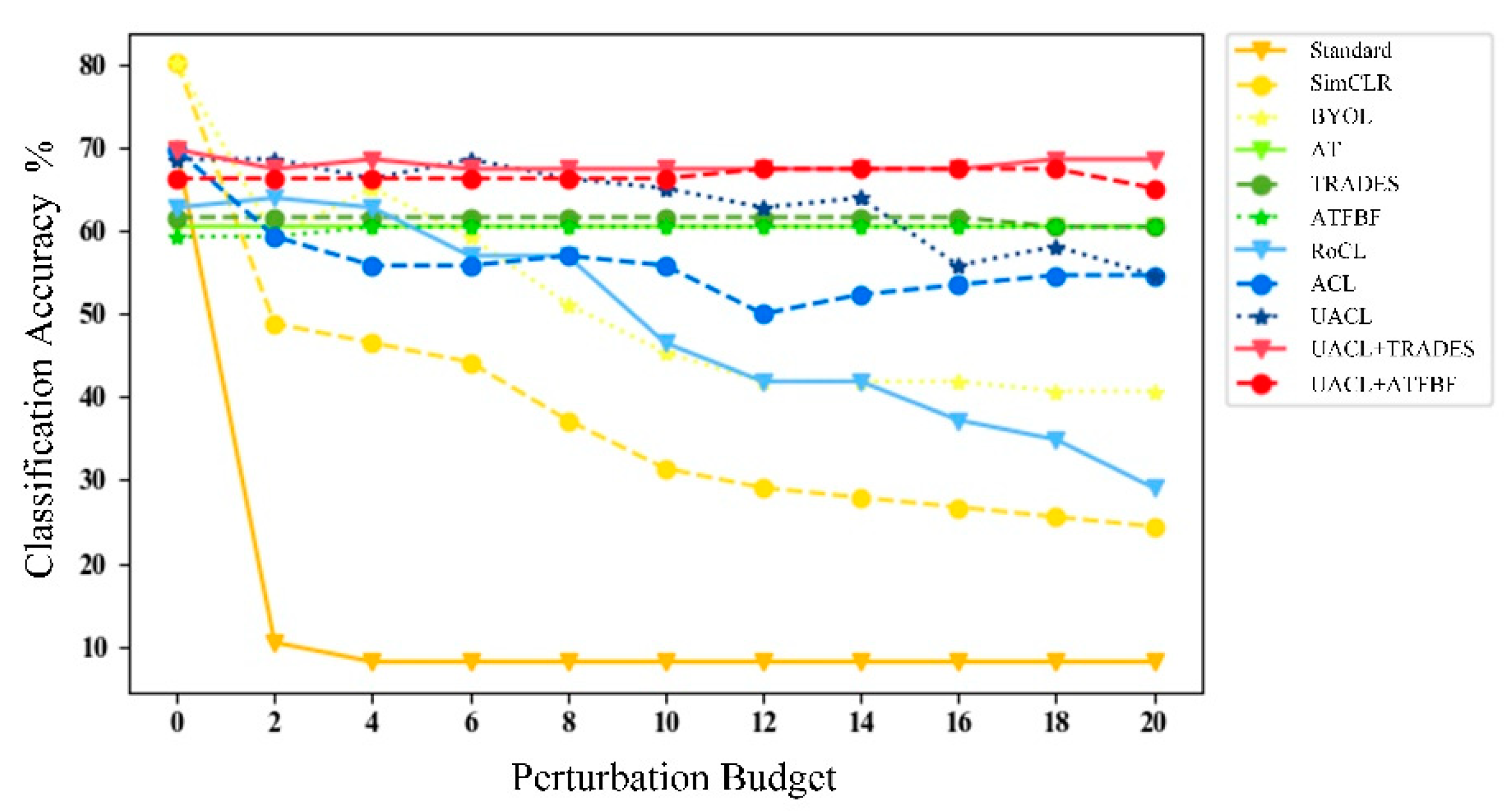
To further research the relation between attack strength and robust accuracy, we utilized a standard adversarial attack ( PGD) with different attack strengths to attack the DNN models. As shown in Figure 7 and Figure 8, adversarial contrastive pretraining defenses, especially UACL, behave better than AT-based defense methods against attacks with low strength. AT-based defense methods can maintain steady robust accuracy as attack strength increases. UACL combined with AT-based defense can lead to stable and excellent robust accuracy in all attack strengths.
Given the lack of labeled SAR image data, we attempted to enhance robustness with a single defense method with only 10% of labeled data and attack the model with PGD, as shown in Table 15. Defense, especially AT-based defenses, will reduce standard accuracy sharply when labeled data are inadequate and adversarial contrastive pretraining defense is significantly better. Adversarial contrastive pretraining defense also performs better in the classification of adversarial examples compared to all AT-based defense methods. Therefore, it should be given priority in the absence of sufficient data. As such, what are the advantages of UACL compared with other adversarial contrastive pretraining defenses such as RoCL and ACL? UACL is faster. The time taken by RoCL, ACL, and UACL to pretrain the model with all data for 200 epochs in our experimental setting is shown in Table 16. We can see that UACL is much faster than RoCL and ACL, as it benefits from the abandonment of negative pairs.
4.5. Visualization of DNNs
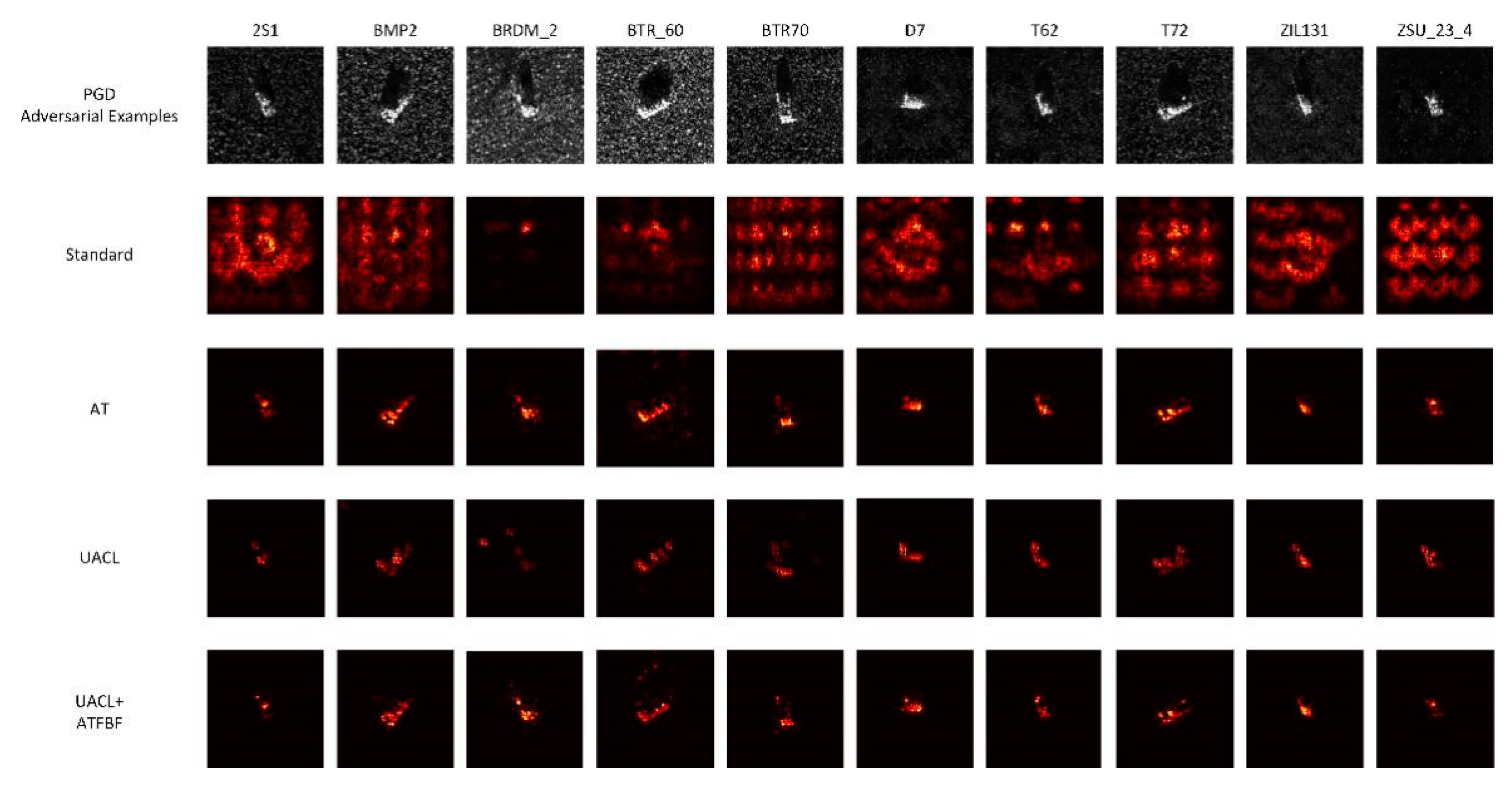
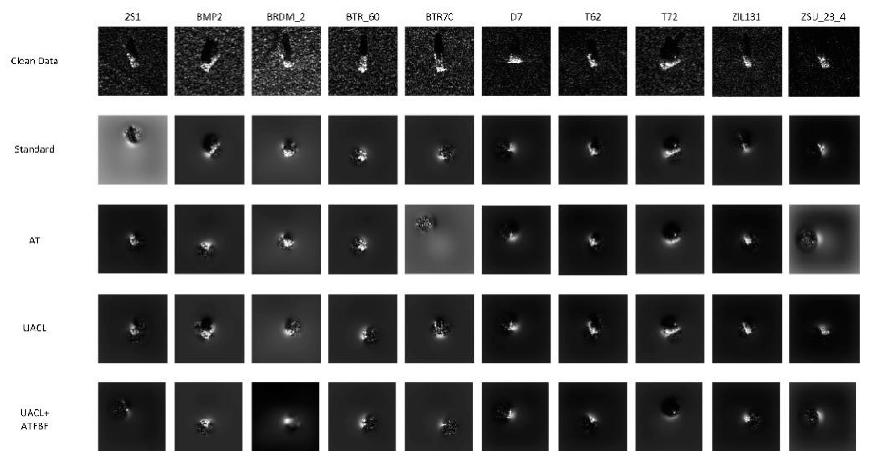
To further understand how defenses improve robust representations, we used guided backpropagation [27] and extremal perturbations [28] to visualize the model and obtain the activation maps of clean images and their PGD adversarial examples.
Guided backpropagation images show which part of the image drives the model to make its final prediction. Guided backpropagation images of MSATR and FUSAR-Ship in standard and adversarial settings are shown in Figure 9, Figure 10, Figure 11 and Figure 12. It can be seen that adversarial examples can effectively destroy the activation of the standard model and make the standard model pay attention to the whole region. The activation region of the standard model is larger both in the face of the clean data and in the adversarial examples. The model with defense will pay more attention to the core region of the image, which improves the adversarial robustness of the model. For a model with AT-based defense (AT), a model with adversarial contrastive pretraining (UACL), and a model with composite defenses (UACL+ATFBF), the active area reduces, in turn showing that the latter has a deeper understanding of the realistic significance of the SAR target.
Extremal perturbations show which part of the image the DNNs pay more attention to. Extremal perturbation images are shown in Figure 13, Figure 14, Figure 15 and Figure 16. It can be seen that the adversarial examples can shift the focus area of the standard model, but not completely change it. Models with adversarial contrastive pretraining can better target the focus area in the face of both the clean data and the adversarial examples, reflecting the advantages and potential of adversarial contrastive pretraining defenses.
5. Conclusions
Robustness is important for SAR target recognition tasks. Although DNNs have achieved great success in SAR target recognition tasks, previous studies have shown that DNN models can be easily fooled by adversarial examples. In this paper, we first systematically evaluated the threat of adversarial examples to DNN-based SAR target recognition models. To alleviate the vulnerability of models to adversarial examples, we then introduced adversarial contrastive pretraining defense into SAR target recognition and proposed a novel unsupervised adversarial contrastive learning defense method. Our experimental results demonstrate that adversarial contrastive pretraining defenses behave well in the classification of both clean data and adversarial examples compared with AT-based defenses, and have great potential to be used in practical applications. Potential future work should include an investigation of the influence of adversarial attacks and defenses on other SAR image datasets and the incorporation of more diverse adversarial self-supervised learning methods.
Author Contributions
Conceptualization, Y.X. and H.S.; methodology, Y.X.; software, Y.X.; validation, H.S., J.C. and L.L.; formal analysis, H.S. and J.C.; investigation, K.J.; resources, L.L. and G.K.; data curation, Y.X.; writing—original draft preparation, Y.X.; writing—review and editing, Y.X. and H.S.; visualization, Y.X.; supervision, H.S.; project administration, G.K.; funding acquisition, H.S. All authors have read and agreed to the published version of the manuscript.
Funding
This work was supported by the National Natural Science Foundation of China under Grant 61971426.
Data Availability Statement
The data presented in this study are available in article. Our codes have been released at: https://github.com/Xu-Yj/Unsupervised-Adversarial-Contrastive-Learning-UACL.
Conflicts of Interest
The authors declare no conflict of interest.
References
- Tait, P. Introduction to Radar Target Recognition; IET: London, UK, 2005; Volume 18. [Google Scholar]
- Xiang, D.; Tang, T.; Ban, Y.; Su, Y. Man-made target detection from polarimetric sar data via nonstationarity and asymmetry. IEEE J. Sel. Top. Appl. Earth Obs. Remote Sens. 2016, 9, 1459–1469. [Google Scholar] [CrossRef]
- Shao, J.; Qu, C.; Li, J. A performance analysis of convolutional neural network models in sar target recognition. In Proceedings of the 2017 SAR in Big Data Era: Models, Methods and Applications (BIGSARDATA), Beijing, China, 13–14 November 2017; pp. 1–6. [Google Scholar]
- Keydel, E.R.; Lee, S.W.; Moore, J.T. Mstar extended operating conditions: A tutorial. In Proceedings of the Algorithms for Synthetic Aperture Radar Imagery III, Orlando, FL, USA, 10 June 1996; pp. 228–242. [Google Scholar]
- Ding, J.; Chen, B.; Liu, H.; Huang, M. Convolutional neural network with data augmentation for sar target recognition. IEEE Geosci. Remote Sens. Lett. 2016, 13, 364–368. [Google Scholar] [CrossRef]
- Ayzel, G.; Heistermann, M.; Sorokin, A.; Nikitin, O.; Lukyanova, O. All convolutional neural networks for radar-based precipitation nowcasting. Procedia Comput. Sci. 2019, 150, 186–192. [Google Scholar] [CrossRef]
- Gu, Y.; Xu, Y. Architecture design of deep convolutional neural network for sar target recognition. J. Image Graph. 2018, 23, 928–936. [Google Scholar]
- Szegedy, C.; Zaremba, W.; Sutskever, I.; Bruna, J.; Erhan, D.; Goodfellow, I.; Fergus, R. Intriguing properties of neural networks. arXiv 2013, arXiv:1312.619. [Google Scholar]
- Xu, Y.; Du, B.; Zhang, L. Assessing the threat of adversarial examples on deep neural networks for remote sensing scene classification: Attacks and defenses. IEEE Trans. Geosci. Remote Sens. 2021, 59, 1604–1617. [Google Scholar] [CrossRef]
- Goodfellow, I.J.; Shlens, J.; Szegedy, C. Explaining and harnessing adversarial examples. arXiv 2014, arXiv:1412.6572. [Google Scholar]
- Moosavi-Dezfooli, S.M.; Fawzi, A.; Frossard, P. Deepfool: A simple and accurate method to fool deep neural networks. In Proceedings of the IEEE Conference on Computer Vision and Pattern Recognition, Las Vegas, NV, USA, 27–30 June 2016; pp. 2574–2582. [Google Scholar]
- Kurakin, A.; Goodfellow, I.; Bengio, S. Adversarial machine learning at scale. In Proceedings of the 5th International Conference on Learning Representations, ICLR - Conference T rack Proceedings, Toulon, France, 24–26 April 2017. [Google Scholar]
- Moosavi-Dezfooli, S.M.; Fawzi, A.; Fawzi, O.; Frossard, P. Universal adversarial perturbations. In Proceedings of the IEEE Conference on Computer Vision and Pattern Recognition, Honolulu, HI, USA, 21–26 July 2017; pp. 1765–1773. [Google Scholar]
- Li, H.; Huang, H.; Chen, L.; Peng, J.; Huang, H.; Cui, Z.; Mei, X.; Wu, G. Adversarial examples for cnn-based sar image classification: An experience study. IEEE J. Sel. Top. Appl. Earth Obs. Remote Sens. 2020, 14, 1333–1347. [Google Scholar] [CrossRef]
- Guo, Y.; Du, L.; Wei, D.; Li, C. Robust sar automatic target recognition via adversarial learning. IEEE J. Sel. Top. Appl. Earth Obs. Remote Sens. 2020, 14, 716–729. [Google Scholar] [CrossRef]
- Chen, T.; Liu, S.; Chang, S.; Cheng, Y.; Amini, L.; Wang, Z. Adversarial robustness: From self-supervised pre-training to fine-tuning. In Proceedings of the IEEE/CVF Conference on Computer Vision and Pattern Recognition, Salt Lake City, UT, USA, 18 June 2018; pp. 699–708. [Google Scholar]
- Hendrycks, D.; Mazeika, M.; Kadavath, S.; Song, D. Using self-supervised learning can improve model robustness and uncertainty. arXiv 2019, arXiv:1906.12340. [Google Scholar]
- Jiang, Z.; Chen, T.; Chen, T.; Wang, Z. Robust pre-training by adversarial contrastive learning. arXiv 2020, arXiv:2010.13337. [Google Scholar]
- Alayrac, J.-B.; Uesato, J.; Huang, P.-S.; Fawzi, A.; Stanforth, R.; Kohli, P. Are labels required for improving adversarial robustness? In Proceedings of the Neural Information Processing Systems, Salt Lake City, UT, USA, 18 June 2018; pp. 12192–12202. [Google Scholar]
- Kim, M.; Tack, J.; Hwang, S.J. Adversarial self-supervised contrastive learning. arXiv 2020, arXiv:2006.07589. [Google Scholar]
- Bui, A.; Le, T.; Zhao, H.; Montague, P.; Camtepe, S.; Phung, D. Understanding and achieving efficient robustness with adversarial contrastive learning. arXiv 2021, arXiv:2101.10027. [Google Scholar]
- Athalye, A.; Carlini, N.; Wagner, D. Obfuscated gradients give a false sense of security: Circumventing defenses to adversarial examples. arXiv 2018, arXiv:1802.00420. [Google Scholar]
- Ortiz-Jiménez, G.; Modas, A.; Moosavi-Dezfooli, S.-M.; Frossard, P. Optimism in the face of adversity: Understanding and improving deep learning through adversarial robustness. arXiv 2020, arXiv:2010.09624. [Google Scholar]
- Czaja, W.; Fendley, N.; Pekala, M.; Ratto, C.; Wang, I.-J. Adversarial examples in remote sensing. In Proceedings of the 26th ACM SIGSPATIAL International Conference on Advances in Geographic Information Systems, Seattle, WA, USA, 6–9 November 2018; pp. 408–411. [Google Scholar]
- Liu, A.; Liu, X.; Guo, J.; Wang, J.; Ma, Y.; Zhao, Z.; Gao, X.; Xiao, G. A comprehensive evaluation framework for deep model robustness. arXiv 2021, arXiv:2101.09617. [Google Scholar]
- He, W.; Li, B.; Song, D. Decision boundary analysis of adversarial examples. In Proceedings of the International Conference on Learning Representations, Vancouver, BC, Canada, 30 April–3 May 2018. [Google Scholar]
- Springenberg, J.T.; Dosovitskiy, A.; Brox, T.; Riedmiller, M. Striving for simplicity: The all convolutional net. arXiv 2014, arXiv:1412.6806. [Google Scholar]
- Fong, R.; Patrick, M.; Vedaldi, A. Understanding deep networks via extremal perturbations and smooth masks. In Proceedings of the IEEE/CVF International Conference on Computer Vision, Seoul, Korea, 27 Octember–2 November 2019; pp. 2950–2958. [Google Scholar]
- Liu, A.; Lin, W.; Paul, M.; Deng, C.; Zhang, F. Just noticeable difference for images with decomposition model for separating edge and textured regions. IEEE Trans. Circuits. Syst. Video Technol. 2010, 20, 1648–1652. [Google Scholar] [CrossRef]
- Tack, J.; Yu, S.; Jeong, J.; Kim, M.; Hwang, S.J.; Shin, J. Consistency regularization for adversarial robustness. arXiv 2021, arXiv:2103.04623. [Google Scholar]
- Chen, T.; Kornblith, S.; Norouzi, M.; Hinton, G. A simple framework for contrastive learning of visual representations. In Proceedings of the IEEE Conference on Computer Vision and Pattern Recognition (CVPR), Seattle, WA, USA, 13–19 June 2020; 2020; pp. 2574–2582. [Google Scholar]
- Zhang, H.; Yu, Y.; Jiao, J.; Xing, E.; El Ghaoui, L.; Jordan, M. Theoretically principled trade-off between robustness and accuracy. In Proceedings of the International Conference on Machine Learning, Long Beach, CA, USA, 10–15 July 2019; pp. 7472–7482. [Google Scholar]
- Wong, E.; Rice, L.; Kolter, J.Z. Fast is better than free: Revisiting adversarial training. arXiv 2020, arXiv:2001.03994 2020. [Google Scholar]
- Hou, X.; Ao, W.; Song, Q.; Lai, J.; Wang, H.; Xu, F. Fusar-ship: Building a high-resolution sar-ais matchup dataset of gaofen-3 for ship detection and recognition. Sci. China Inf. Sci. 2020, 63, 140303. [Google Scholar] [CrossRef] [Green Version]
- Croce, F.; Hein, M. Reliable evaluation of adversarial robustness with an ensemble of diverse parameter-free attacks. In Proceedings of the International Conference on Machine Learning, Las Vegas, NV, USA, November 2020; pp. 2206–2216. [Google Scholar]
- He, K.; Zhang, X.; Ren, S.; Sun, J. Deep Residual Learning for Image Recognition. In Proceedings of the IEEE Conference on Computer Vision and Pattern Recognition, Las Vegas, NV, USA, 27–30 June 2016; pp. 770–778. [Google Scholar]
- Huang, G.; Liu, Z.; Van Der Maaten, L.; Weinberger, K.Q. Densely connected convolutional networks. In Proceedings of the 30th IEEE/CVF Conference on Computer Vision and Pattern Recognition (CVPR), Honolulu, HI, USA, 21–26 July 2017; pp. 4700–4708. [Google Scholar]
- Howard, A.; Zhmoginov, A.; Chen, L.-C.; Sandler, M.; Zhu, M. Inverted residuals and linear bottlenecks: Mobile networks for classification, detection and segmentation. arXiv 2018, arXiv:1801.04381. [Google Scholar]
- Ma, N.; Zhang, X.; Zheng, H.-T.; Sun, J. Shufflenet v2: Practical guidelines for efficient cnn architecture design. arXiv 2018, arXiv:1807.11164. [Google Scholar]
- Feng, S.; Ji, K.; Ma, X.; Zhang, L.; Kuang, G. Target region segmentation in sar vehicle chip image with acm net. IEEE Geosci. Remote Sens. Lett. 2021, 1–5. [Google Scholar] [CrossRef]
Figure 1.
Illustration of adversarial attacks on DNN models for SAR target recognition. The perturbations are amplified ten times for ease of observation.
Figure 1.
Illustration of adversarial attacks on DNN models for SAR target recognition. The perturbations are amplified ten times for ease of observation.

Figure 2.
With 11 evaluation methods in total, our comprehensive robustness evaluation framework focuses on data and model, which are the key factors in an adversarial setting.
Figure 2.
With 11 evaluation methods in total, our comprehensive robustness evaluation framework focuses on data and model, which are the key factors in an adversarial setting.

Figure 3.
Illustration of workflow comparison: (a) AT; (b) RoCL; (c) ACL(DS). Note that RoCL and ACL(DS) share all weights; however, adversarial and standard encoders use independent BN parameters.
Figure 3.
Illustration of workflow comparison: (a) AT; (b) RoCL; (c) ACL(DS). Note that RoCL and ACL(DS) share all weights; however, adversarial and standard encoders use independent BN parameters.

Figure 4.
Illustration of UACL’s architecture. We minimize the similarity loss between the features of augmented data and the corresponding unsupervised adversarial examples to optimize the Siamese network. EMA means exponential moving average. At the end of training, everything but the robust encoder, i.e., the ResNet18, is discarded.

Figure 5.
Example images from the MSTAR dataset.

Figure 6.
Example images from the FUSAR-Ship dataset.

Figure 7.
Robust accuracy of MSTAR models trained with adversarial defense methods against adversarial attacks ( PGD) with different strengths (/255).
Figure 7.
Robust accuracy of MSTAR models trained with adversarial defense methods against adversarial attacks ( PGD) with different strengths (/255).

Figure 8.
Robust accuracy of FUSAR-Ship models trained with adversarial defense methods against adversarial attacks ( PGD) with different strengths (/255).
Figure 8.
Robust accuracy of FUSAR-Ship models trained with adversarial defense methods against adversarial attacks ( PGD) with different strengths (/255).

Figure 9.
Guided backpropagation images of MSTAR model in the classification of clean data.

Figure 10.
Guided backpropagation images of MSTAR model in the classification of adversarial examples.
Figure 10.
Guided backpropagation images of MSTAR model in the classification of adversarial examples.

Figure 11.
Guided backpropagation images of FUSAR-Ship model in the classification of clean data.

Figure 12.
Guided backpropagation images of FUSAR-Ship model in the classification of adversarial examples.
Figure 12.
Guided backpropagation images of FUSAR-Ship model in the classification of adversarial examples.

Figure 13.
Extremal perturbations images of MSTAR model in the classification of clean data.

Figure 14.
Extremal perturbations images of MSTAR model in the classification of adversarial examples.
Figure 14.
Extremal perturbations images of MSTAR model in the classification of adversarial examples.

Figure 15.
Extremal perturbations images of FUSAR-Ship model in the classification of clean data.

Figure 16.
Extremal perturbations images of FUSAR-Ship model in the classification of adversarial examples.
Figure 16.
Extremal perturbations images of FUSAR-Ship model in the classification of adversarial examples.


Table 1.
Details of MSTAR, including target class and data number.
| Target Class | Training Number | Testing Number |
|---|---|---|
| 2S1 | 299 | 274 |
| BMP2 | 233 | 296 |
| BRDM2 | 298 | 274 |
| BTR60 | 256 | 195 |
| BTR70 | 233 | 196 |
| D7 | 299 | 274 |
| T62 | 299 | 273 |
| T72 | 232 | 196 |
| ZIL131 | 299 | 274 |
| ZSU234 | 299 | 274 |
Table 2.
Details of FURSAR-Ship, including target class and data number.
| Target Class | Training Number | Testing Number |
|---|---|---|
| BulkCarrier | 97 | 25 |
| CargoShip | 126 | 32 |
| Fishing | 75 | 19 |
| Tanker | 36 | 10 |
Table 3.
Classification accuracy of MSTAR models against standard adversarial attack (PGD). The adversarial examples can be divided into norm, norm, and norm limited attacks.
Table 3.
Classification accuracy of MSTAR models against standard adversarial attack (PGD). The adversarial examples can be divided into norm, norm, and norm limited attacks.
| Clean Data | Adversarial Examples | ||||||
|---|---|---|---|---|---|---|---|
| 8/255 | 16/255 | 0.25 | 0.5 | 7.84 | 12 | ||
| ResNet18 | 97.65 ± 0.28 | 2.02 ± 0.08 | 1.86 ± 0.04 | 62.60 ± 0.85 | 17.53 ± 0.47 | 86.23 ± 1.33 | 76.87 ± 1.47 |
| ResNet50 | 97.86 ± 0.12 | 1.73 ± 0.07 | 1.65 ± 0.07 | 56.41 ± 0.87 | 19.51 ± 0.68 | 75.18 ± 1.58 | 59.01 ± 1.21 |
| ResNet101 | 98.68 ± 0.25 | 1.53 ± 0.11 | 1.36 ± 0.12 | 56.25 ± 1.16 | 15.13 ± 0.97 | 72.49 ± 1.02 | 57.73 ± 0.93 |
| DenseNet121 | 98.56 ± 0.13 | 0.82 ± 0.08 | 0.37 ± 0.13 | 47.67 ± 2.07 | 6.02 ± 1.28 | 86.35 ± 2.47 | 69.44 ± 1.84 |
| DenseNet201 | 98.68 ± 0.07 | 0.66 ± 0.09 | 0.08 ± 0.15 | 52.82 ± 2.12 | 7.46 ± 1.67 | 84.45 ± 3.11 | 69.94 ± 2.03 |
| MobileNet | 98.23 ± 0.17 | 2.31 ± 0.06 | 1.32 ± 0.07 | 10.31 ± 2.15 | 3.46 ± 1.35 | 67.09 ± 1.09 | 35.09 ± 1.04 |
| ShuffleNet | 95.01 ± 0.78 | 1.48 ± 0.06 | 1.32 ± 0.09 | 9.24 ± 1.45 | 3.09 ± 1.22 | 74.64 ± 1.38 | 23.92 ± 0.79 |
| A-ConvNet | 99.79 ± 0.84 | 0.12 ± 0.01 | 0.12 ± 0.01 | 71.84 ± 2.46 | 17.73 ± 0.38 | 94.39 ± 2.46 | 83.55 ± 2.34 |
| A-ConvNet-M | 98.14 ± 0.33 | 1.98 ± 0.03 | 1.69 ± 0.07 | 68.78 ± 2.73 | 21.85 ± 1.52 | 87.05 ± 1.10 | 73.15 ± 1.22 |
Table 4.
Classification accuracy of FUSAR-Ship models against standard adversarial attack (PGD).
| Clean Data | Adversarial Examples | ||||||
|---|---|---|---|---|---|---|---|
| 8/255 | 16/255 | 0.25 | 0.5 | 7.84 | 12 | ||
| ResNet18 | 69.77 ± 2.32 | 8.14 ± 2.32 | 8.14 ± 2.32 | 16.28 ± 2.32 | 13.95 ± 2.32 | 53.49 ± 3.49 | 37.21 ± 3.49 |
| ResNet50 | 68.60 ± 3.49 | 4.65 ± 1.16 | 4.65 ± 1.16 | 13.95 ± 2.32 | 12.79 ± 1.16 | 50.00 ± 2.32 | 37.21 ± 2.32 |
| ResNet101 | 70.93 ± 4.65 | 29.07 ± 2.32 | 29.07 ± 2.32 | 25.58 ± 3.49 | 20.93 ± 2.32 | 53.49 ± 3.49 | 45.35 ± 2.32 |
| DenseNet121 | 66.28 ± 4.65 | 24.42 ± 2.32 | 24.42 ± 2.32 | 11.63 ± 2.32 | 6.98 ± 1.16 | 59.30 ± 3.49 | 41.86 ± 3.49 |
| DenseNet201 | 68.60 ± 4.65 | 29.06 ± 3.49 | 29.07 ± 2.32 | 30.23 ± 3.49 | 24.42 ± 2.32 | 68.60 ± 2.32 | 55.81 ± 3.49 |
| MobileNet | 63.95 ± 4.65 | 29.07 ± 4.65 | 29.07 ± 2.32 | 20.93 ± 1.16 | 20.93 ± 1.16 | 22.09 ± 1.16 | 23.26 ± 2.32 |
| ShuffleNet | 45.35 ± 5.81 | 26.74 ± 3.49 | 26.74 ± 2.32 | 29.07 ± 2.32 | 29.07 ± 3.49 | 38.37 ± 2.32 | 36.05 ± 2.32 |
| A-ConvNet | 81.34 ± 3.49 | 5.81 ± 2.32 | 5.81 ± 2.32 | 48.83 ± 3.49 | 26.74 ± 2.32 | 63.95 ± 2.32 | 56.98 ± 3.49 |
| A-ConvNet-M | 70.93 ± 2.32 | 25.58 ± 4.65 | 25.58 ± 2.32 | 31.39 ± 2.32 | 26.74 ± 3.49 | 43.02 ± 3.49 | 36.05 ± 2.32 |
Table 5.
Classification accuracy of MSTAR models against different kinds of adversarial attack.
| Method | Clean Data | PGD | FGSM | APGD | Deep Fool | CW | Sparse-RS | Sparse Fool | Square Attack | Hop Skip Jump |
|---|---|---|---|---|---|---|---|---|---|---|
| ResNet18 | 97.65 ± 0.28 | 2.02 ± 0.08 | 3.01 ± 0.57 | 2.02 ± 0.05 | 2.10 ± 0.06 | 14.85 ± 0.79 | 63.59 ± 0.84 | 51.76 ± 0.86 | 70.47 ± 2.44 | 13.81 ± 0.76 |
| ResNet50 | 97.86 ± 0.12 | 1.73 ± 0.07 | 9.61 ± 0.66 | 1.32 ± 0.05 | 1.94 ± 0.13 | 12.29 ± 0.47 | 62.93 ± 0.92 | 50.98 ± 0.69 | 58.68 ± 1.76 | 9.36 ± 0.55 |
| ResNet101 | 98.68 ± 0.25 | 1.53 ± 0.11 | 12.33 ± 0.93 | 1.36 ± 0.07 | 1.73 ± 0.26 | 10.56 ± 0.77 | 61.94 ± 0.95 | 48.98 ± 0.93 | 60.66 ± 1.57 | 14.72 ± 0.87 |
| DenseNet121 | 98.56 ± 0.13 | 0.82 ± 0.08 | 6.14 ± 1.64 | 0.82 ± 0.09 | 1.32 ± 0.14 | 18.68 ± 1.56 | 60.70 ± 1.21 | 50.32 ± 0.98 | 57.24 ± 1.22 | 8.74 ± 0.58 |
| DenseNet201 | 98.68 ± 0.07 | 0.66 ± 0.09 | 6.02 ± 1.06 | 0.62 ± 0.09 | 1.03 ± 0.25 | 16.29 ± 1.36 | 60.82 ± 1.09 | 51.30 ± 0.90 | 48.00 ± 0.74 | 16.33 ± 0.80 |
| MobileNet | 98.23 ± 0.17 | 2.31 ± 0.06 | 4.58 ± 0.60 | 2.10 ± 0.05 | 3.38 ± 0.20 | 31.30 ± 2.32 | 45.61 ± 0.83 | 41.26 ± 0.84 | 47.96 ± 0.49 | 9.40 ± 0.48 |
| ShuffleNet | 95.01 ± 0.78 | 1.48 ± 0.06 | 2.10 ± 0.49 | 1.32 ± 0.06 | 1.73 ± 0.08 | 29.69 ± 2.14 | 42.64 ± 0.42 | 41.09 ± 0.68 | 48.16 ± 0.83 | 9.07 ± 0.74 |
| A-ConvNet | 99.79 ± 0.84 | 0.12 ± 0.01 | 0.16 ± 0.01 | 0.08 ± 0.01 | 0.16 ± 0.01 | 16.41 ± 0.92 | 71.05 ± 1.24 | 69.03 ± 1.22 | 39.59 ± 0.66 | 3.79 ± 0.32 |
| A-ConvNet-M | 98.14 ± 0.03 | 1.98 ± 0.03 | 8.78 ± 0.87 | 1.94 ± 0.07 | 3.75 ± 0.14 | 83.34 ± 2.56 | 67.84 ± 1.07 | 68.11 ± 1.01 | 17.36 ± 0.82 | 10.47 ± 0.54 |
Table 6.
Classification accuracy of FUSAR-Ship models against different kinds of adversarial attack.
Table 6.
Classification accuracy of FUSAR-Ship models against different kinds of adversarial attack.
| Method | Clean Data | PGD | FGSM | APGD | Deep Fool | CW | Sparse-RS | Sparse Fool | Square Attack | Hop Skip Jump |
|---|---|---|---|---|---|---|---|---|---|---|
| ResNet18 | 69.77 ± 2.32 | 8.14 ± 2.32 | 29.07 ± 2.32 | 8.14 ± 1.16 | 22.09 ± 1.16 | 19.77 ± 2.32 | 12.79 ± 1.16 | 33.72 ± 2.32 | 69.77 ± 2.32 | 24.42 ± 2.32 |
| ResNet50 | 68.60 ± 3.49 | 4.65 ± 1.16 | 29.07 ± 2.32 | 5.81 ± 1.16 | 20.93 ± 2.32 | 26.74 ± 2.32 | 13.95 ± 1.16 | 33.72 ± 2.32 | 68.60 ± 3.49 | 4.65 ± 1.16 |
| ResNet101 | 70.93 ± 4.65 | 29.07 ± 2.32 | 44.19 ± 2.32 | 26.74 ± 2.32 | 23.26 ± 2.32 | 32.56 ± 1.16 | 40.70 ± 2.32 | 38.37 ± 3.49 | 70.93 ± 4.65 | 29.07 ± 2.32 |
| DenseNet121 | 66.28 ± 4.65 | 24.42 ± 2.32 | 17.44 ± 1.16 | 8.14 ± 2.32 | 20.93 ± 1.16 | 24.42 ± 2.32 | 30.23 ± 2.32 | 50.00 ± 3.49 | 66.28 ± 4.65 | 24.42 ± 2.32 |
| DenseNet201 | 68.60 ± 4.65 | 29.06 ± 3.49 | 29.07 ± 2.32 | 5.81 ± 1.16 | 20.93 ± 1.16 | 27.91 ± 3.16 | 19.77 ± 2.32 | 43.03 ± 2.32 | 68.60 ± 4.65 | 29.06 ± 3.49 |
| MobileNet | 63.95 ± 4.65 | 29.07 ± 4.65 | 29.07 ± 2.32 | 16.28 ± 2.32 | 47.67 ± 3.49 | 25.58 ± 1.16 | 22.09 ± 1.16 | 33.72 ± 2.32 | 63.95 ± 4.65 | 29.07 ± 4.65 |
| ShuffleNet | 45.35 ± 5.81 | 26.74 ± 3.49 | 19.77 ± 2.32 | 15.12 ± 2.32 | 38.37 ± 1.16 | 37.21 ± 3.16 | 30.23 ± 2.32 | 38.37 ± 3.49 | 45.35 ± 5.81 | 26.74 ± 3.49 |
| A-ConvNet | 81.34 ± 3.49 | 5.81 ± 2.32 | 40.70 ± 3.49 | 9.30 ± 2.32 | 36.04 ± 2.32 | 8.14 ± 1.16 | 36.05 ± 1.16 | 12.79 ± 2.32 | 81.34 ± 3.49 | 5.81 ± 2.32 |
| A-ConvNet-M | 70.93 ± 2.32 | 25.58 ± 4.65 | 26.74 ± 2.32 | 23.26 ± 2.32 | 23.26 ± 1.16 | 41.86 ± 4.65 | 48.84 ± 2.32 | 13.95 ± 3.49 | 70.93 ± 2.32 | 25.58 ± 4.65 |
Table 7.
Comprehensive evaluation of different DNN models against PGD attack (attack strength is 8/255 in norm) in MSTAR dataset.
Table 7.
Comprehensive evaluation of different DNN models against PGD attack (attack strength is 8/255 in norm) in MSTAR dataset.
| SA | RA | ACAC | RCAC | NTE | EBD | ALPp | ASS | PSD | TKNC | |||
|---|---|---|---|---|---|---|---|---|---|---|---|---|
| L0 | L2 | |||||||||||
| ResNet18 | 97.65 | 2.02 | 0.99 | 685 | 0.99 | 1.66 | 0.97 | 685 | 8 | 0.83 | 423 | 0.11 |
| ResNet50 | 97.86 | 1.73 | 1.00 | inf | 1.00 | 1.55 | 0.97 | 917 | 8 | 0.84 | 415 | 0.03 |
| ResNet101 | 98.68 | 1.53 | 1.00 | inf | 1.00 | 1.66 | 0.97 | 914 | 8 | 0.84 | 414 | 0.03 |
| DenseNet121 | 98.56 | 0.82 | 0.99 | 1470 | 0.98 | 1.66 | 0.95 | 880 | 8 | 0.85 | 392 | 0.03 |
| DenseNet201 | 98.68 | 0.66 | 0.99 | 1668 | 0.98 | 1.66 | 0.96 | 897 | 8 | 0.84 | 402 | 0.02 |
| MobileNet | 98.23 | 2.31 | 0.99 | 1514 | 0.98 | 1.66 | 0.94 | 789 | 8 | 0.86 | 342 | 0.03 |
| ShuffleNet | 95.01 | 1.48 | 0.99 | 1474 | 0.98 | 1.52 | 0.95 | 830 | 8 | 0.84 | 364 | 0.06 |
| A-ConvNet | 99.79 | 0.12 | 1.0 | inf | 1.0 | 1.66 | 0.96 | 862 | 8 | 0.84 | 385 | 0.23 |
| A-ConvNet-M | 98.14 | 1.98 | 1.00 | inf | 1.0 | 1.66 | 0.94 | 819 | 8 | 0.84 | 385 | 0.18 |
Table 8.
Comprehensive evaluation of different DNN models against PGD attack (attack strength is 8/255 in norm) in FUSAR-Ship dataset.
Table 8.
Comprehensive evaluation of different DNN models against PGD attack (attack strength is 8/255 in norm) in FUSAR-Ship dataset.
| SA | RA | ACAC | RCAC | NTE | EBD | ALPp | ASS | PSD | TKNC | |||
|---|---|---|---|---|---|---|---|---|---|---|---|---|
| L0 | L2 | |||||||||||
| ResNet18 | 69.77 | 8.14 | 1.00 | inf | 1.00 | 1.30 | 0.92 | 2924 | 8.00 | 0.38 | 6153 | 0.07 |
| ResNet50 | 68.60 | 6.98 | 1.00 | inf | 1.00 | 1.30 | 0.97 | 3641 | 8.00 | 0.39 | 6834 | 0.04 |
| ResNet101 | 70.93 | 20.93 | 0.99 | inf | 1.00 | 1.85 | 0.96 | 3485 | 8.00 | 0.29 | 6445 | 0.01 |
| DenseNet121 | 66.28 | 24.42 | 1.00 | inf | 1.00 | 1.59 | 0.97 | 3667 | 8.00 | 0.35 | 6915 | 0.01 |
| DenseNet201 | 68.60 | 10.47 | 1.00 | inf | 1.00 | 1.85 | 0.97 | 3509 | 8.00 | 0.29 | 6515 | 0.01 |
| MobileNet | 63.95 | 29.07 | 1.00 | inf | 1.00 | 1.85 | 0.98 | 3821 | 8.00 | 0.35 | 7338 | 0.01 |
| ShuffleNet | 45.35 | 26.74 | 1.00 | inf | 1.00 | 1.79 | 0.98 | 3571 | 8.00 | 0.28 | 6675 | 0.02 |
| A-ConvNet | 81.34 | 5.81 | 1.00 | inf | 1.00 | 1.59 | 0.97 | 3762 | 8.00 | 0.35 | 6343 | 0.01 |
| A-ConvNet-M | 70.93 | 26.74 | 0.99 | inf | 1.00 | 1.85 | 0.94 | 3145 | 8.00 | 0.35 | 6934 | 0.01 |
Table 9.
Classification accuracy of models (ResNet18) with no-defense or defense methods against PGD adversarial attacks in MSTAR dataset.
Table 9.
Classification accuracy of models (ResNet18) with no-defense or defense methods against PGD adversarial attacks in MSTAR dataset.
| Clean Data | Adversarial Examples | |||||||
|---|---|---|---|---|---|---|---|---|
| 8/255 | 16/255 | 0.25 | 0.5 | 7.84 | 12 | |||
| No Defense | Standard | 97.65 ± 0.28 | 2.02 ± 0.11 | 1.86 ± 0.08 | 62.60 ± 0.68 | 17.53 ± 0.77 | 86.23 ± 1.44 | 76.87 ± 1.11 |
| SimCLR | 99.38 ± 0.19 | 22.93 ± 0.74 | 2.27 ± 0.54 | 97.65 ± 0.92 | 93.15 ± 0.69 | 98.56 ± 1.20 | 98.35 ± 1.01 | |
| BYOL | 99.51 ± 0.22 | 29.15 ± 0.66 | 4.99 ± 0.51 | 97.28 ± 0.99 | 93.24 ± 0.88 | 98.43 ± 1.23 | 97.94 ± 0.78 | |
| Defense | AT | 86.23 ± 1.59 | 79.13 ± 0.74 | 69.98 ± 0.61 | 85.11 ± 1.24 | 84.33 ± 0.93 | 85.57 ± 0.97 | 85.36 ± 0.55 |
| TRADES | 90.85 ± 0.86 | 80.87 ± 0.83 | 66.02 ± 0.77 | 90.14 ± 1.09 | 88.45 ± 0.69 | 90.56 ± 1.54 | 80.87 ± 0.98 | |
| ATFBF | 86.02 ± 0.58 | 84.41 ± 0.67 | 82.06 ± 0.53 | 84.29 ± 1.10 | 84.49 ± 0.79 | 83.75 ± 1.29 | 84.12 ± 0.69 | |
| RoCL | 92.43 ± 0.95 | 80.73 ± 0.82 | 65.40 ± 0.76 | 88.16 ± 1.33 | 90.29 ± 0.90 | 89.65 ± 0.93 | 89.10 ± 0.69 | |
| ACL | 95.34 ± 1.33 | 74.43 ± 0.44 | 51.88 ± 0.35 | 88.99 ± 2.22 | 83.59 ± 1.20 | 90.19 ± 1.49 | 90.43 ± 0.93 | |
| UACL | 95.09 ± 0.90 | 80.92 ± 0.89 | 60.74 ± 0.54 | 94.10 ± 2.04 | 93.36 ± 0.80 | 94.31 ± 1.10 | 94.27 ± 0.90 | |
| UACL+TRADES | 90.02 ± 0.48 | 87.88 ± 0.62 | 84.91 ± 0.44 | 89.73 ± 1.79 | 89.53 ± 0.77 | 89.98 ± 0.92 | 89.90 ± 0.53 | |
| UACL+ ATFBF | 96.99 ± 0.29 | 95.38 ± 0.60 | 92.16 ± 0.38 | 96.86 ± 1.53 | 96.66 ± 0.74 | 97.03 ± 0.88 | 97.03 ± 0.47 | |
Table 10.
Classification accuracy of models (ResNet18) with no-defense or defense methods against PGD adversarial attacks in FUSAR-Ship dataset.
Table 10.
Classification accuracy of models (ResNet18) with no-defense or defense methods against PGD adversarial attacks in FUSAR-Ship dataset.
| Clean Data | Adversarial Examples | |||||||
|---|---|---|---|---|---|---|---|---|
| 8/255 | 16/255 | 0.25 | 0.5 | 7.84 | 12 | |||
| No Defense | Standard | 69.77 ± 2.32 | 8.14 ± 2.32 | 8.14 ± 2.32 | 16.28 ± 2.32 | 13.95 ± 2.32 | 53.49 ± 3.49 | 37.21 ± 3.49 |
| SimCLR | 80.23 ± 5.81 | 37.21 ± 2.32 | 26.74 ± 2.32 | 47.67 ± 2.32 | 47.67 ± 3.49 | 40.70 ± 2.32 | 46.51 ± 3.49 | |
| BYOL | 80.23 ± 5.81 | 51.16 ± 2.32 | 41.86 ± 3.49 | 59.30 ± 3.49 | 58.14 ± 3.49 | 59.30 ± 3.49 | 59.30 ± 4.65 | |
| Defense | AT | 60.47 ± 2.32 | 60.47 ± 3.49 | 60.47 ± 2.32 | 60.47 ± 4.65 | 60.47 ± 4.65 | 60.47 ± 4.65 | 60.47 ± 3.49 |
| TRADES | 61.63 ± 3.49 | 61.63 ± 3.49 | 61.63 ± 3.49 | 61.63 ± 4.65 | 61.63 ± 4.65 | 61.63 ± 4.65 | 61.63 ± 3.49 | |
| ATFBF | 59.30 ± 2.32 | 60.47 ± 4.65 | 60.47 ± 2.32 | 59.30 ± 3.49 | 59.30 ± 3.49 | 59.30 ± 4.65 | 59.30 ± 4.65 | |
| RoCL | 62.79 ± 2.32 | 56.98 ± 3.49 | 37.21 ± 2.32 | 61.63 ± 5.81 | 61.63 ± 3.49 | 62.79 ± 5.81 | 62.79 ± 5.81 | |
| ACL | 69.77 ± 3.49 | 56.98 ± 5.81 | 53.49 ± 2.32 | 72.09 ± 5.81 | 69.77 ± 5.81 | 70.93 ± 5.81 | 70.93 ± 5.81 | |
| UACL | 68.60 ± 2.32 | 65.12 ± 3.49 | 55.81 ± 2.32 | 67.44 ± 3.49 | 67.44 ± 4.65 | 68.60 ± 3.49 | 68.60 ± 4.65 | |
| UACL+TRADES | 69.77 ± 2.32 | 67.44 ± 4.65 | 68.60 ± 5.81 | 68.60 ± 4.65 | 68.60 ± 4.65 | 69.77 ± 5.81 | 69.77 ± 4.65 | |
| UACL+ ATFBF | 66.28 ± 3.49 | 66.28 ± 4.65 | 67.44 ± 5.81 | 66.28 ± 4.65 | 66.28 ± 4.65 | 66.28 ± 4.65 | 66.28 ± 3.49 | |
Table 11.
Classification accuracy of models (ResNet18) with no-defense or defense methods against different kinds of adversarial attack in MSTAR dataset.
Table 11.
Classification accuracy of models (ResNet18) with no-defense or defense methods against different kinds of adversarial attack in MSTAR dataset.
| PGD | FGSM | APGD | DeepFool | CW | Sparse-RS | Sparsefool | SquareAttack | HopSkipJump | ||
|---|---|---|---|---|---|---|---|---|---|---|
| No Defense | Standard | 2.02 ± 0.11 | 3.01 ± 0.34 | 2.02 ± 0.09 | 2.10 ± 0.09 | 14.85 ± 1.29 | 63.59 ± 1.08 | 51.76 ± 1.46 | 70.47 ± 0.86 | 13.81 ± 0.32 |
| SimCLR | 22.93 ± 0.74 | 47.22 ± 0.59 | 19.34 ± 0.50 | 36.70 ± 0.09 | 93.57 ± 0.53 | 74.89 ± 1.22 | 60.33 ± 1.46 | 55.96 ± 0.53 | 46.35 ± 0.89 | |
| BYOL | 29.15 ± 0.66 | 58.10 ± 0.56 | 26.93 ± 0.33 | 30.19 ± 0.09 | 97.20 ± 1.16 | 76.16 ± 1.40 | 61.09 ± 1.46 | 71.22 ± 0.76 | 67.88 ± 0.96 | |
| Defense | AT | 79.13 ± 0.74 | 81.53 ± 0.98 | 79.84 ± 0.42 | 74.14 ± 0.09 | 84.91 ± 1.29 | 84.91 ± 1.31 | 81.93 ± 1.46 | 85.32 ± 0.92 | 86.10 ± 0.94 |
| TRADES | 80.87 ± 0.83 | 85.03 ± 1.20 | 81.98 ± 0.54 | 75.01 ± 0.09 | 89.24 ± 1.79 | 89.11 ± 1.57 | 85.31 ± 1.46 | 89.81 ± 0.98 | 90.35 ± 1.02 | |
| ATFBF | 84.41 ± 0.67 | 83.59 ± 0.97 | 83.26 ± 0.47 | 81.07 ± 0.09 | 83.67 ± 1.60 | 84.08 ± 1.30 | 84.24 ± 1.46 | 83.30 ± 0.67 | 83.55 ± 0.89 | |
| RoCL | 80.73 ± 0.82 | 86.02 ± 0.84 | 76.29 ± 0.70 | 81.07 ± 0.09 | 90.38 ± 1.57 | 90.55 ± 1.69 | 88.49 ± 1.46 | 84.08 ± 1.24 | 91.90 ± 1.23 | |
| ACL | 74.43 ± 0.44 | 79.53 ± 0.68 | 59.98 ± 0.31 | 68.60 ± 0.09 | 80.62 ± 1.01 | 87.42 ± 1.64 | 82.10 ± 1.46 | 82.14 ± 1.08 | 86.52 ± 1.20 | |
| UACL | 80.92 ± 0.89 | 85.20 ± 1.14 | 76.33 ± 0.66 | 81.53 ± 0.09 | 93.20 ± 1.32 | 93.07 ± 1.89 | 93.07 ± 1.46 | 85.15 ± 1.33 | 92.33 ± 1.08 | |
| UACL+TRADES | 87.88 ± 0.62 | 88.66 ± 0.92 | 87.92 ± 0.68 | 86.47 ± 0.09 | 89.65 ± 1.05 | 89.40 ± 1.02 | 89.67 ± 1.46 | 89.53 ± 1.03 | 89.65 ± 1.01 | |
| UACL+ ATFBF | 95.38 ± 0.60 | 95.92 ± 0.77 | 95.55 ± 0.53 | 88.29 ± 0.09 | 96.82 ± 1.10 | 95.22 ± 0.77 | 95.18 ± 1.46 | 96.91 ± 0.93 | 96.99 ± 0.92 |
Table 12.
Classification accuracy of models (ResNet18) with no-defense or defense methods against different kinds of adversarial attack in FUSAR-Ship dataset.
Table 12.
Classification accuracy of models (ResNet18) with no-defense or defense methods against different kinds of adversarial attack in FUSAR-Ship dataset.
| PGD | FGSM | APGD | DeepFool | CW | Sparse-RS | Sparsefool | SquareAttack | HopSkipJump | ||
|---|---|---|---|---|---|---|---|---|---|---|
| No Defense | Standard | 8.14 ± 2.32 | 19.77 ± 2.32 | 8.14 ± 1.16 | 29.07 ± 2.32 | 19.77 ± 2.32 | 38.49 ± 2.32 | 36.90 ± 3.49 | 12.79 ± 2.32 | 34.88 ± 2.32 |
| SimCLR | 37.21 ± 2.32 | 46.51 ± 2.32 | 53.49 ± 3.49 | 47.67 ± 2.32 | 47.67 ± 3.49 | 53.49 ± 3.49 | 46.51 ± 4.65 | 17.44 ± 2.32 | 53.49 ± 4.65 | |
| BYOL | 51.16 ± 2.32 | 40.70 ± 2.32 | 48.84 ± 2.32 | 58.14 ± 3.49 | 55.81 ± 4.65 | 46.51 ± 2.32 | 40.70 ± 3.49 | 46.51 ± 4.65 | 48.84 ± 4.65 | |
| Defense | AT | 60.47 ± 3.49 | 60.47 ± 2.32 | 60.47 ± 3.49 | 60.47 ± 3.49 | 60.47 ± 4.65 | 60.47 ± 3.49 | 60.47 ± 5.81 | 60.47 ± 3.49 | 60.47 ± 2.32 |
| TRADES | 61.63 ± 3.49 | 61.63 ± 3.49 | 61.63 ± 3.49 | 61.63 ± 4.65 | 61.63 ± 4.65 | 61.63 ± 3.49 | 61.63 ± 4.65 | 62.79 ± 3.49 | 61.63 ± 3.49 | |
| ATFBF | 60.47 ± 4.65 | 60.47 ± 3.49 | 60.47 ± 2.32 | 59.30 ± 3.49 | 59.30 ± 3.49 | 59.30 ± 2.32 | 59.30 ± 4.65 | 60.47 ± 3.49 | 60.47 ± 2.32 | |
| RoCL | 56.98 ± 3.49 | 46.51 ± 4.65 | 54.65 ± 3.49 | 62.79 ± 3.49 | 62.79 ± 4.65 | 59.30 ± 4.65 | 55.81 ± 5.81 | 58.14 ± 5.81 | 56.98 ± 5.81 | |
| ACL | 56.98 ± 5.81 | 26.74 ± 4.65 | 33.72 ± 4.65 | 70.93 ± 5.81 | 70.93 ± 4.65 | 61.63 ± 4.65 | 59.30 ± 5.81 | 30.23 ± 5.81 | 55.81 ± 5.81 | |
| UACL | 65.12 ± 3.49 | 62.79 ± 3.49 | 63.95 ± 3.49 | 68.60 ± 4.65 | 69.77 ± 3.49 | 68.60 ± 3.49 | 68.60 ± 4.65 | 56.98 ± 3.49 | 55.81 ± 4.65 | |
| UACL+TRADES | 67.44 ± 4.65 | 67.44 ± 4.65 | 67.44 ± 3.49 | 69.77 ± 4.65 | 69.77 ± 4.65 | 69.77 ± 3.49 | 69.77 ± 4.65 | 68.60 ± 4.65 | 70.93 ± 3.49 | |
| UACL+ ATFBF | 66.28 ± 4.65 | 66.28 ± 4.65 | 67.44 ± 2.32 | 66.28 ± 3.49 | 66.28 ± 3.49 | 66.28 ± 2.32 | 66.28 ± 4.65 | 67.44 ± 3.49 | 67.44 ± 3.49 |
Table 13.
Comprehensive evaluation of models (ResNet18) with no-defense or defense methods against PGD attacks (attack strength is 8/255 in norm) in MSTAR dataset.
Table 13.
Comprehensive evaluation of models (ResNet18) with no-defense or defense methods against PGD attacks (attack strength is 8/255 in norm) in MSTAR dataset.
| SA | RA | ACAC | RCAC | NTE | EBD | PSD | TKNC | ||
|---|---|---|---|---|---|---|---|---|---|
| No Defense | Standard | 97.65 | 2.02 | 0.998 | 685 | 0.996 | 1.66 | 423 | 0.11 |
| SimCLR | 99.38 | 22.93 | 0.916 | 27.6 | 0.841 | 1.66 | 427 | 0.49 | |
| BYOL | 99.51 | 29.15 | 0.927 | 29.0 | 0.863 | 1.60 | 423 | 0.47 | |
| Defense | AT | 86.23 | 79.13 | 0.491 | 1.4 | 0.142 | 1.67 | 422 | 0.41 |
| TRADES | 90.85 | 80.87 | 0.563 | 1.8 | 0.247 | 1.67 | 424 | 0.39 | |
| ATFBF | 86.02 | 84.41 | 0.540 | 1.6 | 0.194 | 1.67 | 441 | 0.49 | |
| RoCL | 92.43 | 80.73 | 0.691 | 41.4 | 0.855 | 1.66 | 423 | 0.51 | |
| ACL | 95.34 | 34.43 | 0.629 | 13.6 | 0.698 | 1.67 | 422 | 0.57 | |
| UACL | 95.09 | 80.92 | 0.661 | 9.8 | 0.742 | 1.64 | 433 | 0.56 | |
| UACL+TRADES | 90.02 | 87.88 | 0.526 | 1.4 | 0.161 | 1.50 | 418 | 0.58 | |
| UACL+ ATFBF | 96.99 | 95.38 | 0.787 | 3.8 | 0.579 | 1.67 | 403 | 0.43 |
Table 14.
Comprehensive evaluation of models (ResNet18) with no-defense or defense methods against PGD attacks (attack strength is 8/255 in norm) in FUSAR-Ship dataset. Because the robust accuracy of some models is not less than the standard accuracy, some parameters cannot be obtained.
Table 14.
Comprehensive evaluation of models (ResNet18) with no-defense or defense methods against PGD attacks (attack strength is 8/255 in norm) in FUSAR-Ship dataset. Because the robust accuracy of some models is not less than the standard accuracy, some parameters cannot be obtained.
| SA | RA | ACAC | RCAC | NTE | EBD | PSD | TKNC | ||
|---|---|---|---|---|---|---|---|---|---|
| No Defense | Standard | 69.77 | 8.14 | 1 | inf | 1 | 1.30 | 6153 | 0.07 |
| SimCLR | 80.23 | 37.21 | 0.84 | 9.10 | 0.70 | 1.21 | 5173 | 0.05 | |
| BYOL | 80.23 | 51.16 | 0.81 | 10.4 | 0.77 | 1.14 | 5802 | 0.04 | |
| Defense | AT | 60.47 | 60.47 | \ | \ | \ | 1.77 | \ | 0.02 |
| TRADES | 61.63 | 61.63 | \ | \ | \ | 1.80 | \ | 0.03 | |
| ATFBF | 59.30 | 60.47 | \ | \ | \ | 1.74 | \ | 0.03 | |
| RoCL | 62.79 | 56.98 | 0.65 | 3.56 | 0.35 | 1.59 | 4598 | 0.03 | |
| ACL | 69.77 | 56.98 | 0.70 | 7.33 | 0.34 | 1.62 | 4794 | 0.03 | |
| UACL | 68.60 | 65.12 | 0.61 | 2.02 | 0.31 | 1.68 | 4560 | 0.03 | |
| UACL+TRADES | 69.77 | 67.44 | 0.50 | 1.01 | 0.01 | 1.74 | 4992 | 0.03 | |
| UACL+ ATFBF | 66.28 | 66.28 | \ | \ | \ | 1.42 | \ | 0.03 |
Table 15.
Classification accuracy of models (ResNet18) with different defense methods trained with 10% labeled data against PGD adversarial attacks.
Table 15.
Classification accuracy of models (ResNet18) with different defense methods trained with 10% labeled data against PGD adversarial attacks.
| Clean data | PGD(ε = 8/255) | PGD(ε = 16/255) | |
|---|---|---|---|
| Standard | 77.15 | 2.02 | 2.02 |
| AT | 42.76 | 42.64 | 42.72 |
| TRADES | 40.87 | 37.77 | 37.90 |
| ATFTF | 41.24 | 40.99 | 41.03 |
| RoCL | 63.42 | 62.02 | 61.77 |
| ACL | 68.20 | 47.90 | 45.18 |
| UACL | 64.45 | 62.35 | 61.28 |
Table 16.
The training times of adversarial contrastive pretraining defenses.
| RoCL | ACL | UACL | |
|---|---|---|---|
| MSTAR | 25:01:24 | 29:12:36 | 17:28:14 |
| FUSAR-Ship | 7:12:09 | 5:34:56 | 4:09:40 |
Publisher’s Note: MDPI stays neutral with regard to jurisdictional claims in published maps and institutional affiliations. |
© 2021 by the authors. Licensee MDPI, Basel, Switzerland. This article is an open access article distributed under the terms and conditions of the Creative Commons Attribution (CC BY) license (https://creativecommons.org/licenses/by/4.0/).
Share and Cite
MDPI and ACS Style
Xu, Y.; Sun, H.; Chen, J.; Lei, L.; Ji, K.; Kuang, G. Adversarial Self-Supervised Learning for Robust SAR Target Recognition. Remote Sens. 2021, 13, 4158. https://0-doi-org.brum.beds.ac.uk/10.3390/rs13204158
AMA Style
Xu Y, Sun H, Chen J, Lei L, Ji K, Kuang G. Adversarial Self-Supervised Learning for Robust SAR Target Recognition. Remote Sensing. 2021; 13(20):4158. https://0-doi-org.brum.beds.ac.uk/10.3390/rs13204158
Chicago/Turabian StyleXu, Yanjie, Hao Sun, Jin Chen, Lin Lei, Kefeng Ji, and Gangyao Kuang. 2021. "Adversarial Self-Supervised Learning for Robust SAR Target Recognition" Remote Sensing 13, no. 20: 4158. https://0-doi-org.brum.beds.ac.uk/10.3390/rs13204158
Note that from the first issue of 2016, this journal uses article numbers instead of page numbers. See further details here.