
Important Airborne Lidar Metrics of Canopy Structure for Estimating Snow Interception


1
Clark School of Environment and Sustainability, Western Colorado University, Gunnison, CO 81231, USA
2
McCall Outdoor Science School, College of Natural Resources, University of Idaho, McCall, ID 83638, USA
3
Department of Forest, Rangeland and Fire Sciences, College of Natural Resources, University of Idaho, Moscow, ID 83843, USA
4
School of Forest Resources and Conservation, University of Florida, Gainesville, FL 32611, USA
*
Author to whom correspondence should be addressed.
Remote Sens. 2021, 13(20), 4188; https://0-doi-org.brum.beds.ac.uk/10.3390/rs13204188
Submission received: 16 September 2021
/
Revised: 15 October 2021
/
Accepted: 16 October 2021
/
Published: 19 October 2021
Abstract
:Forest canopies exert significant controls over the spatial distribution of snow cover. Canopy snow interception efficiency is controlled by intrinsic processes (e.g., canopy structure), extrinsic processes (e.g., meteorological conditions), and the interaction of intrinsic-extrinsic factors (i.e., air temperature and branch stiffness). In hydrological models, intrinsic processes governing snow interception are typically represented by two-dimensional metrics like the leaf area index (LAI). To improve snow interception estimates and their scalability, new approaches are needed for better characterizing the three-dimensional distribution of canopy elements. Airborne laser scanning (ALS) provides a potential means of achieving this, with recent research focused on using ALS-derived metrics that describe forest spacing to predict interception storage. A wide range of canopy structural metrics that describe individual trees can also be extracted from ALS, although relatively little is known about which of them, and in what combination, best describes intrinsic canopy properties known to affect snow interception. The overarching goal of this study was to identify important ALS-derived canopy structural metrics that could help to further improve our ability to characterize intrinsic factors affecting snow interception. Specifically, we sought to determine how much variance in canopy intercepted snow volume can be explained by ALS-derived crown metrics, and what suite of existing and novel crown metrics most strongly affects canopy intercepted snow volume. To achieve this, we first used terrestrial laser scanning (TLS) to quantify snow interception on 14 trees. We then used these snow interception measurements to fit a random forest model with ALS-derived crown metrics as predictors. Next, we bootstrapped 1000 calculations of variable importance (percent increase in mean squared error when a given explanatory variable is removed), keeping nine canopy metrics for the final model that exceeded a variable importance threshold of 0.2. ALS-derived canopy metrics describing intrinsic tree structure explained approximately two-thirds of the snow interception variability (R2 ≥ 0.65, RMSE ≤ 0.52 m3, relative RMSE ≤ 48%) in our study when extrinsic factors were kept as constant as possible. For comparison, a generalized linear mixed-effects model predicting snow interception volume from LAI alone had a marginal R2 = 0.01. The three most important predictor variables were canopy length, whole-tree volume, and unobstructed returns (a novel metric). These results suggest that a suite of intrinsic variables may be used to map interception potential across larger areas and provide an improvement to interception estimates based on LAI.
1. Introduction
Forests within the northern hemisphere are estimated to contain 20% of global winter snow cover and 17% of global winter freshwater storage [1,2]. The structure and arrangement of the forest canopy is a major factor controlling the distribution of snow, as well as runoff rates and volumes [3]. Canopy intercepted snow can account for up to 60% of the total annual snowfall, depending on forest type, forest structural properties, and meteorological conditions [4,5], with subsequent sublimation as high as 25–50% in cold, dry environments [6,7]. Canopy-interception processes are thus important to consider when modeling the hydrology of snow-dependent regions and their water supplies [8].
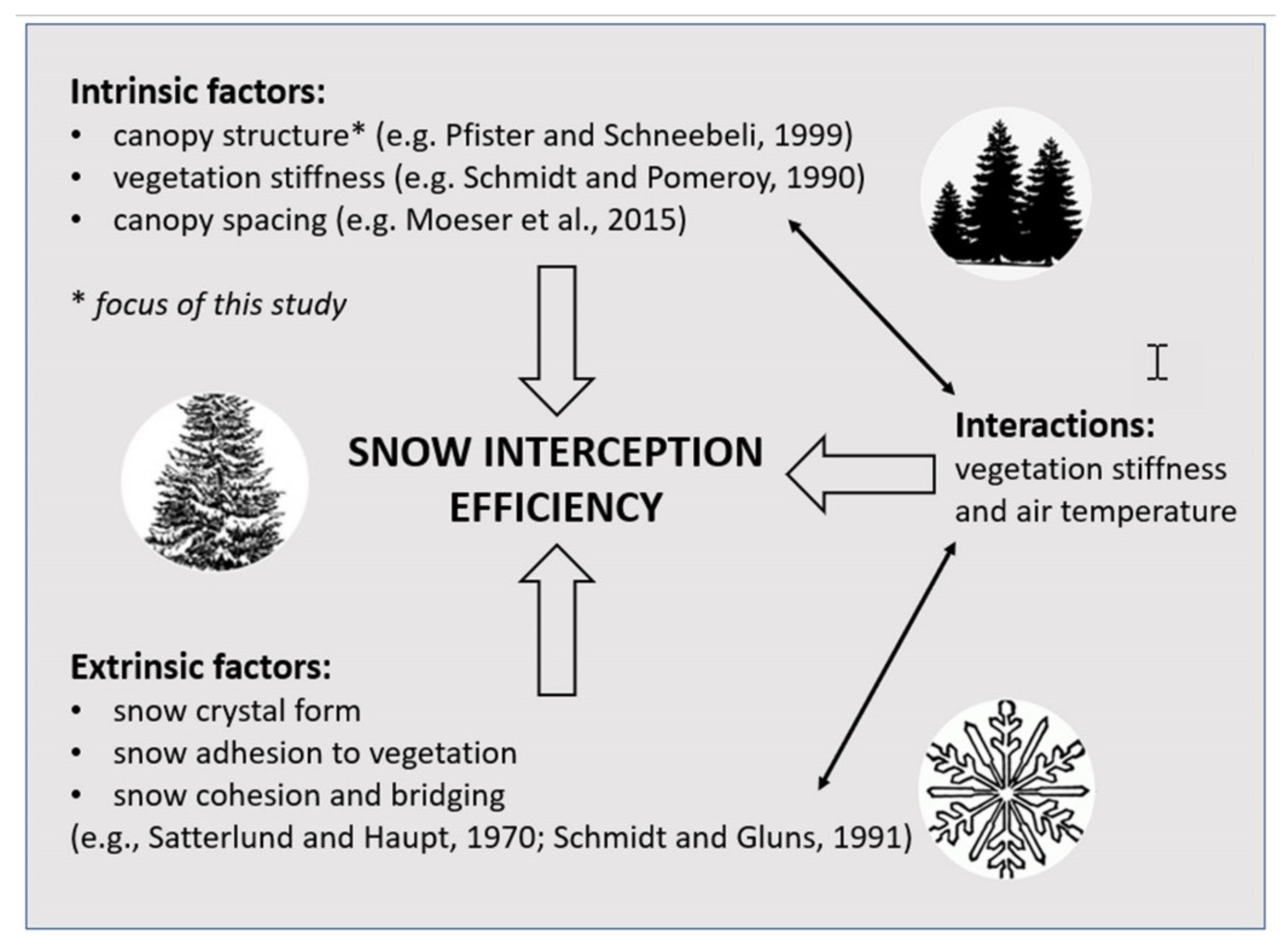
Despite its importance as a variable in hydrological models [2,9,10], accurately estimating snow interception remains challenging due to complex interactions between intrinsic and extrinsic factors (Figure 1). Intrinsic structural factors like branch/canopy arrangement and vegetation stiffness and their effect on snow storage dynamics have been studied at the branch level with physical models [11,12], excised branches [13], and time-lapse video [14]. These studies described how branch architecture influences micro-scale (sub-centimeter) mechanisms that control how and where snow accumulates, as well as the rate of accumulation. For example, Pfister and Schneebeli [12] found that snow interception efficiency increased with the width of the branch due to reduced snow crystal rebound near the edges, and irregularly shaped branch models with low inclination angles had significantly higher accumulations. Schmidt and Gluns [13] observed how differences in branch structure between conifer species affect mechanisms of snow interception efficiency (e.g., crystal rebound, snow bridging), although meteorological conditions produced greater differences in snow interception. Indeed, snow interception is also partially controlled by extrinsic hydrometeorological factors (e.g., air temperature, snow water content, wind speed, etc.) that affect crystal type, snow adhesion to vegetation, and bridging of snow due to cohesion [15]. Furthermore, the interaction between extrinsic air temperature and intrinsic branch flexibility affects snow interception efficiency through the process of mass unloading [16].
To estimate snow interception, tree-scale measurements (e.g., data from load cells, lysimeters, and pressure sensors) have been made (e.g., [5,7,17]). Scaling up measurements of whole-tree interception is problematic, however, because the methods are resource intensive and may not be representative across complex terrain. Alternatively, snow interception estimates obtained indirectly by comparing forested and non-forested sites are prone to error due to confounding processes (e.g., wind redistribution of snow and branch unloading) [3,18]. Recent studies have examined the length scale of forest edge effects on snowpack variability [19], and the control snow-depth variability exerts on the occurrence of trees [20], but have not addressed snow interception directly. Due to these challenges, most hydrological models infer snow interception from two-dimensional metrics of canopy architecture like the leaf area index (LAI) or canopy closure (CC) [2,9], data that are relatively easy to obtain from in situ field observations or remote sensing [21,22]. Interception is partitioned from total snowfall by estimating the maximum snow load that can be captured by a canopy as an empirical function of LAI (e.g., [7]). The authors of the Snow Model Intercomparison Project 2 (SNOWMIP2) [2,9] reported that most of the 33 models of forest-snow processes they examined rely on LAI to predict maximum interception. They cautioned that they found inconsistency in the methods used to calculate LAI. In addition, although many of the models employ the empirical equation used in Hedstrom and Pomeroy [7] that defines the LAI-interception relationship, there is inconsistency in how this scheme is implemented [23] and concern that it may underpredict snow interception in environments outside the boreal forest zone where it was developed [17]. Beyond the aforementioned issues, both LAI and CC also do not capture the fundamental three-dimensional (3-D) spatial arrangement of canopy features that accounts for the intrinsic baseline snow interception efficiency [11,12]. Hence, to improve snow interception estimates and their scalability, approaches are needed that characterize the 3-D arrangement of canopy elements, a key intrinsic factor known to affect canopy interception [24] at multiple scales.
Airborne laser scanning (ALS), commonly known as lidar (light detection and ranging), presents a potential means of achieving this. For each survey point that reflects an emitted laser beam back to the ALS sensor, a datalogger records spherical coordinates (distance from scanner, azimuth angle, polar angle) that are later converted to Cartesian x,y,z coordinates, as well as the return intensity of the laser beam [25]. A point cloud contains all of these spatial coordinates and is subsequently utilized for classifying and mapping the 3-D structural properties of Earth surface features, such as the terrain, forests, and snow cover [26,27,28,29]. Mazzotti and colleagues [30] utilized ALS to extract a spatially continuous canopy metric (distance to canopy edge), finding that it performed better than CC for a continental snow environment and could be aggregated to the watershed scale. Zheng et al. [31] found that canopy metrics extracted from ALS (e.g., mean canopy height, canopy cover fractions, etc.) explained approximately 50% of the variability of snow accumulation on the ground. Addressing snow interception specifically, Moeser and colleagues [32] combined an underlying snow interception efficiency distribution with ALS-derived estimates of LAI, CC, tree size, and novel intrinsic metrics of canopy spacing (i.e., forest gap size and horizontal position) to model snow interception in a continental snow environment. They found a 27% increase in model fit (R2 = 0.66) when compared to previous models at the point scale (e.g., [7]). Furthermore, Moeser and colleagues [33] found that the ‘total gap area’ (average R = 0.78) was more highly correlated with interception than LAI (average R = 0.57), and that intrinsic overhead canopy elements are more important than extrinsic snowfall intensity in predicting maximum interception. Roth and Nolin [18] extended this modeling approach by modifying the ALS-derived intrinsic variables (e.g., gap length) to integrate information on the vertical position in space and focusing on two extrinsic variables (i.e., snowfall, air temperature). They found that, in a maritime snow environment, forest structure sets the baseline potential or likelihood of a given forest to intercept, with air temperature influencing the rate of interception.
These studies demonstrate the potential for modeling snow interception based on ALS-derived information on intrinsic forest spacing (e.g., gaps), extrinsic meteorological data, and indirect validation data. In addition, intrinsic factors affecting snow interception could be characterized with canopy structural metrics of individual trees derived from ALS. ALS-derived canopy structural metrics are widely employed for the efficient estimation of forest biomass across large areas [34,35]. For example, Means and colleagues [35] used ALS to estimate forest structural parameters (e.g., tree height percentiles, basal area, tree volume) over a Douglas fir-dominated temperate forest in western Oregon, finding good correspondence with field validation data (R2 = 0.93-0.98). Other studies extracted metrics from canopy vertical profiles, including height and volume distributions [36,37,38]. All these studies demonstrate the wide range of different canopy structural metrics that can be derived from ALS, but relatively little is known about which of them, and what combination best describes intrinsic canopy properties known to affect snow interception. This is due, in part, to the difficulty of efficiently obtaining validation data of interception variability across a range of trees. Yet, recent research advances suggest that terrestrial laser scanning (TLS) could be a valuable validation tool for directly mapping and quantifying snow interception in field plots [39].
The overarching goal of this study was to identify important ALS-derived crown-level structural metrics that could help to further improve our ability to characterize intrinsic factors affecting snow interception. Specifically, our objectives were as follows: 1) determine how much variance in canopy intercepted snow volume can be explained by ALS-derived crown-level metrics; and 2) identify a suite of existing and novel crown metrics that are most strongly correlated with canopy intercepted snow volume. The outcomes of this study will provide insights into what canopy structural information from lidar remote sensing could best contribute to the effort to further improve the modeling and monitoring of snow interception storage across larger spatial scales.
2. Materials and Methods
2.1. Field Data
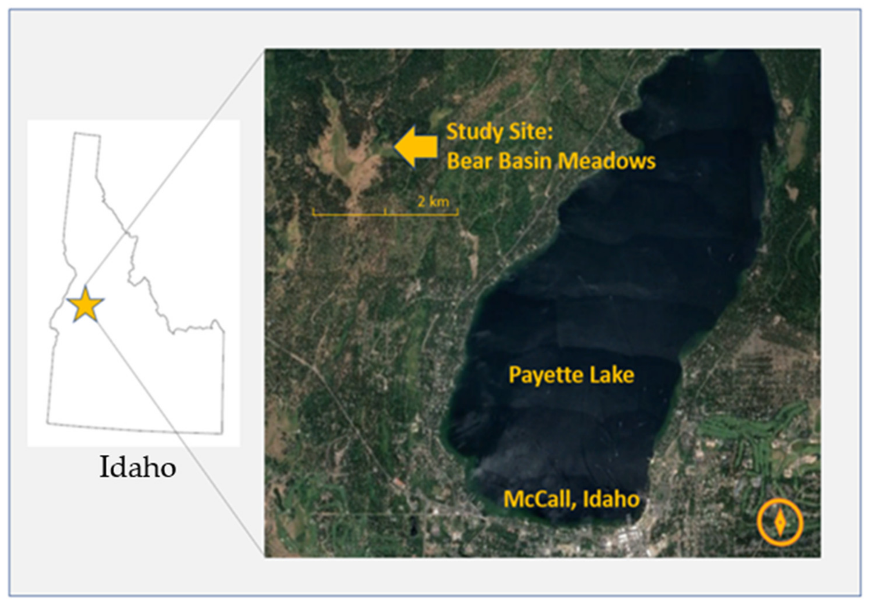
Field data were collected at Bear Basin Meadows in the Payette National Forest (McCall Ranger District) near McCall, Idaho at 1640 m elevation (Figure 2). Bear Basin Meadows is a large meadow complex surrounded by montane forest in the mountains of west-central Idaho.
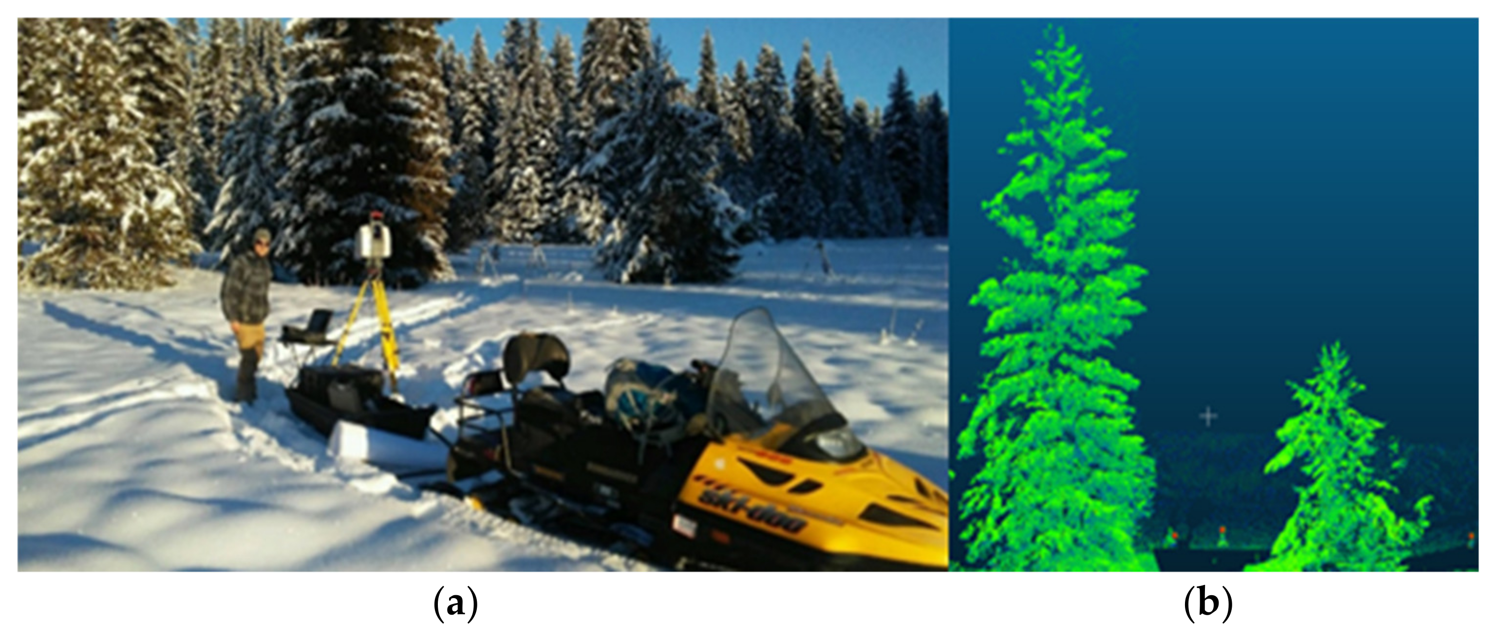
Fourteen snow-free trees of varying size classes (maximum height = 31.7 m; minimum height = 1.4 m; mean height = 11.7 m; standard deviation = 9.6 m) and structural forms (e.g., maximum width = 13.9 m; minimum width = 2.6 m; mean width = 8.1 m; standard deviation = 3.3 m) were scanned with a Leica Scan Station 2 (Leica Geosystems AG Heerbrugg, Switzerland) TLS (distance accuracy ± 4 mm with 0.15 mrad beam divergence) on October 25, 2018. Trees (Pseudotsuga menziesii (n = 2), Pinus contorta (n = 10), Pinus ponderosa (n = 2)) were visually selected to represent variance in structure (e.g., canopy height, width, distribution of vegetation on stem, etc.) rather than species. The trees are all in open forest (i.e., minimal subcanopy) along the margins of a meadow. The distances between our study trees and the nearest neighboring trees (i.e., nearest neighbor distance) was an average of 4.4 m (0.2 m minimum, 12.7 m maximum). To fully capture the structural complexity of each tree, two scans were made from opposing sides of each tree (0.005 m horizontal/vertical scan resolution at 5 m) and included three TLS targets for co-registration of the scenes. To maximize the variance in the structure, scans included individual trees or small clumps of trees that were processed as one tree. Two subsequent snow-on data collections were performed on December 5, 2018 and January 1, 2019, during which the same methods were repeated (Figure 3). The Bear Basin snow telemetry station (National Resource and Conservation Service SNOTEL Site #319), approximately 600 m from the study site, reported mean air temperature during daylight hours was −11.2°C on December 5th, with a maximum air temperature of −6.4°C and snow depth on the ground surface measuring 13 cm. The mean air temperature during daylight hours was −9.0°C on January 1, with a maximum air temperature of −6.2°C and snow depth on the ground surface measuring 71 cm. Snowfall prior to each snow-on data collection consisted of approximately 20 cm on December 2nd and 5 cm on December 31st. We attempted to control for extrinsic factors affecting our results by scanning all trees during the same day under similar weather conditions (i.e., subfreezing, low wind) and in the same general area, thereby assuming that variability in the interception between trees would primarily be caused by intrinsic factors. The mean wind speed at the McCall airport (5 km distant) between the onset of snowfall and the first sampling event was 4.5 km per hour (maximum sustained 16.1 km per hour); mean wind speed between the onset of snowfall and the second sampling event was 3.5 km per hour (maximum sustained 24.8 km per hour). The wind speeds preceding sampling suggest low rates of wind-induced offloading and sublimation, although it is not known how much (if any) snow was on the trees prior to the most recent snowfall event.
2.2. TLS Data Preprocessing and Canopy-Level Intercepted Snow Volume Estimation
Using the three TLS targets, point clouds acquired from two sides of a tree were registered with the ‘three point picking’ tool in the open source software package CloudCompare (version 2.10.2) [40]. After registration, each point cloud was subsampled to a 0.05 m minimal point spacing to allow for uniform comparability throughout the individual tree canopies and between different trees. The subsampling distance was selected to reflect the point spacing in the crown of the tallest tree sampled (i.e., furthest distance from the scanner to the target). To approximate a relative increase in volume with snow loading independent of confounding factors like occlusions due to laser absorption/scattering [26,39,41] and branch deflection [16], “snow off” point clouds were added to their corresponding “snow on” point clouds using the automated registration within CloudCompare [40]. The point clouds were then transformed into convex hulls in R [42] using the ‘alphashape3d’ R package [43], which approximates the shape and volume of the scanned structure. The convexity parameter (α) was set to 0.05 m to match the point spacing of the underlying data. Only the upper 75% of each point cloud was utilized to construct convex hulls, excluding canopy components that were occluded by the snowpack and ice attached to the lowest portion of the tree canopies. Next, snow-free tree volumes were subtracted from snow-on tree volumes to calculate volumes of intercepted snow. This approach for approximating snow volume from TLS data was validated by integrating the methodology into data from Russell et al. [44]. The resulting model regression demonstrated good agreement between the estimated TLS-derived snow interception and snow interception quantified by a load cell (R2 = 0.68, RMSE = 1.66 m3, slope = 1.55, intercept = -3.71). Finally, a Welch two-sample t-test was utilized to test whether or not the means of the December and January samples were significantly different.
2.3. Calculation of Standard Crown Metrics from Aerial Laser Scanning
Aerial lidar data for the Bear Basin study site were downloaded from the “The National Map” [45]. Data were acquired on March 15, 2018 for the United States Geological Survey (USGS) 3DEP LiDAR Project using a Leica ALS80 system (Leica Geosystems AG Heerbrugg, Switzerland) at an altitude of 1800 m (22 mrad beam divergence, 30° field of view, 39.6 cm laser pulse footprint diameter). The average first-return point density was 18.00 points/m2, the average ground-return point density was 2.93 points/m2, and RMSE was 0.37 m when compared to a bare earth digital elevation model. The aerial lidar tile encompassing the Bear Basin study site has a minimum elevation of 1587 m and a maximum elevation of 1952 m. CloudCompare [40] was used to clip ALS-derived shapefiles corresponding to the 14 sampled trees.
The CrownMetrics function in the ‘rLiDAR’ package [46] was used to produce 11 structural canopy metrics (e.g., maximum height, mean height, etc.) for each sample tree. The normalmixEM function from the ‘mixtools’ R package [47] was employed to calculate the crown base height from the vertical profiles of heights within the crown polygon. The chullLiDAR3D function in ‘rLiDAR’ [46] was used to produce 3-D convex hulls derived from ALS returns within the crown segments and calculate the crown surface area and volume. The ‘alphashape3D’ package [43] was utilized to calculate whole-tree volumes for three arbitrary α values (α = 0.25, 0.50, 0.75) spanning the α range (0 – 1). Twenty-three total standard canopy metrics were included in subsequent modeling (see Table 1 for definitions). Crown-level metrics based on laser return intensities were excluded as candidate variables because they have been thought to be mainly sensitive to extrinsic factors (e.g., [26,41]) of snow interception, which is not the focus of this study. See Section 3 for additional metrics that were excluded from the final model on the basis of irrelevance to snow interception processes.
2.4. Calculation of Novel Canopy Metrics from Aerial Laser Scanning
Original metrics that quantify the number of unobstructed (i.e., first return) and obstructed returns (height values less than the first return) (Table 1) were produced as a proxy for the amount of vegetative structure on the exterior surfaces of trees. These metrics follow the principle that the first surfaces snow crystals encounter are the most likely to intercept and accumulate snow; snow accumulation in the interior of the canopy is limited to snow crystals that slide down steeply angled branches to accumulate at branch attachments to the trunk [12] or deposit in high wind/wet snow conditions [48]. The unobstructed returns (UNOB) metric is a count of first returns only. The UNOBDK metric weights overlapping returns with an exponential decay function in which:
where n is the number of overlapping returns within the laser footprint (39.6 cm in this study, see Section 2.3).
subtract = 0.0498*exp(0.5 * n),
“Subtract” is the value to be subtracted from the total number of returns in the point cloud. If the number of overlapping returns exceeds six, then a value of one is subtracted; overlapping returns exceeding six result in high subtract values and an illogical negative/low total count of first returns. The exponential decay function accounts for the assumption that the likelihood of intercepting snow decreases exponentially with the number of canopy layers. Percent unobstructed returns (UNOB%) and percent unobstructed returns with decay function (UNOBDK%) present UNOB and UNOBDK values as a ratio of the total returns. Although the exponential expression used here may appear somewhat arbitrary, the authors deemed it a worthwhile inclusion in the model because it addresses a mechanistic property of snow interception [12,13] and would potentially inspire future research into snow interception-specific canopy metrics if found significant.
2.5. Analysis
To address our first objective of determining how much variance in canopy intercepted snow volume is explained by ALS-derived canopy metrics, we fitted a random forest (RF) model between observed TLS-derived snow volumes estimates and ALS-derived structural metrics. RF is a non-parametric machine learning approach that makes no assumptions about the distribution/independence of variables [49] and can accommodate many predictor variables relative to the number of observations, with each individual predictor providing limited information [50]. The random forest approach we used built 1000 regression trees that each utilize only a subset of predictors and observations. One run, the bootstrap sample, is the data chosen to be “in-the-bag” for sampling with replacement; the “out-of-bag” (i.e., out-of-sample) data is all values not chosen for the run. Repeating this process 1000 times distributes variable importance across all correlated predictors, and is thus robust against overfitting and multicollinearity [49,51,52]. Predictions from all the trees were combined for estimates of model variance and error, estimates that therefore integrate a conservative modeling approach utilizing out-of-sample data. While RF modeling may appear challenging to the casual reader, it is increasingly employed in a wide variety of applications using freely available software and was the most appropriate choice given the nature of the snow interception dataset. All RF models were fit with the ‘randomForest’ R package [53] with the default settings for mtry (i.e., the number of predictors sampled at each node: 1/3 of total predictors) and ntree (i.e., the number of regression trees grown for each RF run) set to 1000. Because our second objective was identifying lidar structural metrics best suited to help predict intercepted snow volume, we did not reduce our model to include only predictor variables below a certain correlation threshold (e.g., R = 0.9 in Genuer et al. [54]). Instead, we relied on RF estimates of variable importance to determine the most parsimonious model. Variable importance is a measure of the increase in mean squared error (MSE) when a given explanatory variable is removed [55]. To account for stochasticity in variable importance estimates [53,56], we iterated the calculation 1000 times (bootstrapped without replacement). Variables that exceeded a 0.2 variable importance threshold, a default value in many RF modeling applications [57], across all runs were retained for fitting of the final RF model.
Predicted values of the snow interception volume were produced by the final RF model in predict mode. To determine how much variance in canopy intercepted snow volume can be explained by ALS-derived crown metrics (objective 1), we regressed observed (i.e., TLS-derived) against predicted snow interception volume and evaluated the precision and accuracy of the model based on the coefficient of determination (R2) and root mean squared error (RMSE)/relative RMSE, respectively. Having identified the suite of existing and novel crown metrics that most strongly affect canopy intercepted snow volume (objective 2), we then ranked the final suite of variables by importance (i.e., % increase MSE if removed was from the model).
3. Results
Estimates of snow interception (volume) from December 5th ranged between 0.15 and 4.48 m3 per individual tree (mean 1.20 m3; standard deviation 2.26 m3). Estimates of snow interception from January 1st ranged between 0.08 and 2.64 m3 (mean 0.98 m3; standard deviation 1.30 m3). Higher snow volume estimates were recorded for 12 of 14 trees on December 5th compared to January 1st. A Welch two sample t-test showed that the means of each sample were not significantly different (t = 0.967, df = 27.634, p-value = 0.171 with a 95% confidence interval).
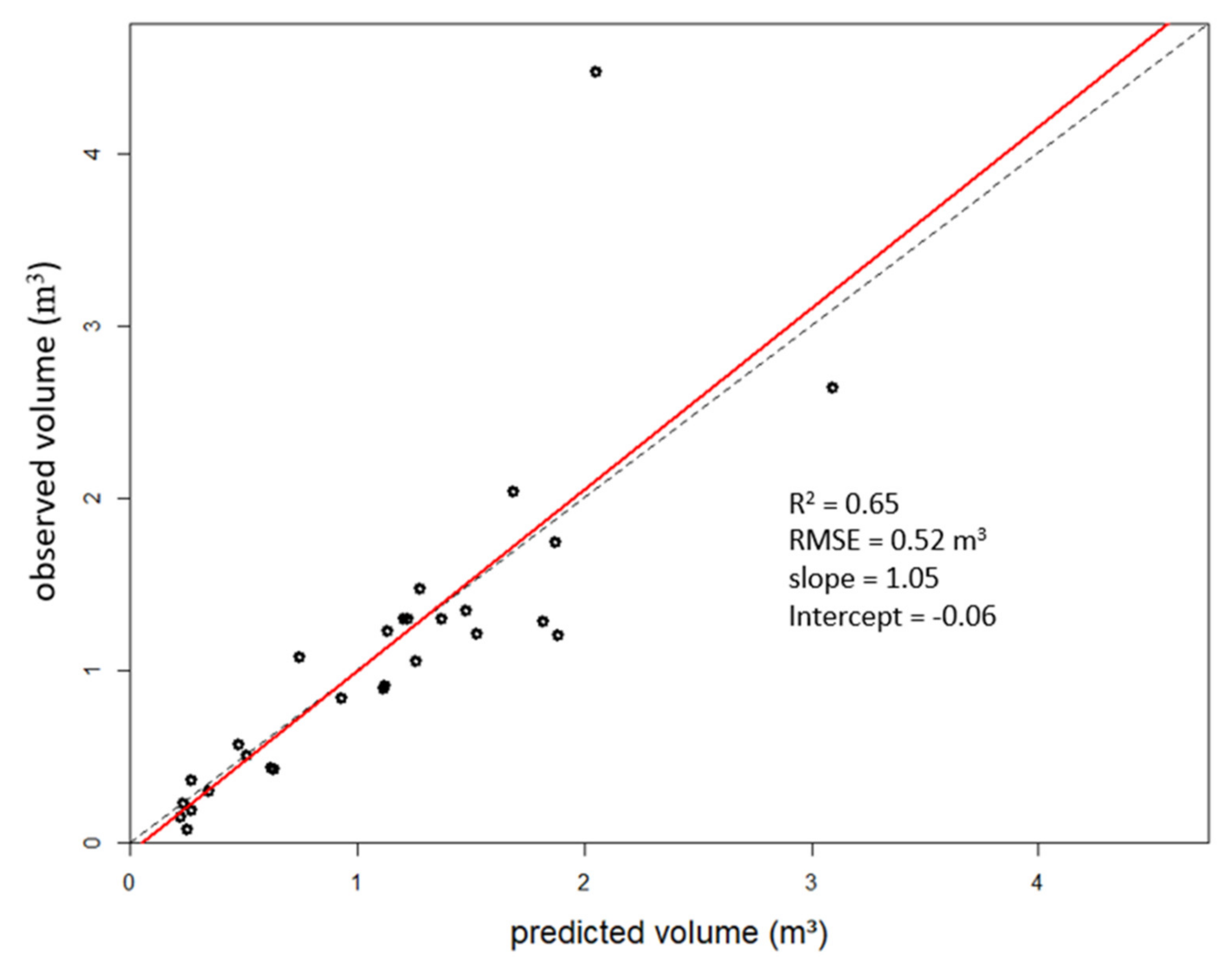
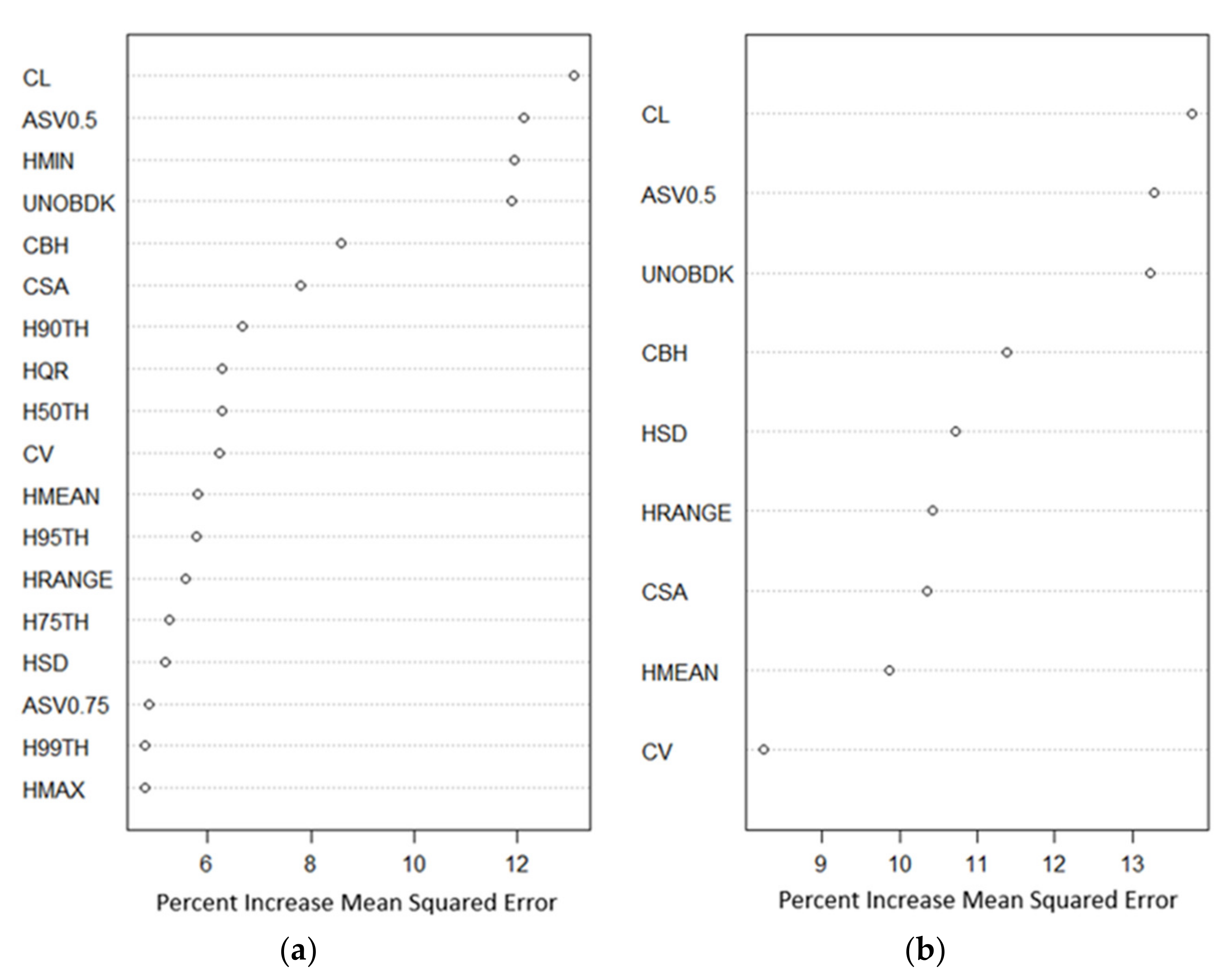
The RF model with all standard variables included produced the following estimates of model fit and error: R2 = 0.65 and RMSE = 0.52 m3. After iteratively calculating the variable importance 1000 times (bootstrapped without replacement), 10 out of 28 variables were removed from the model for not exceeding the 0.2 variable importance threshold across all runs. Next, HMIN and the remaining height percentile metrics (e.g., HQR, H25TH, H50th, etc.) were removed because they did not add meaningfully to the interpretation of modeling results in the context of snow interception processes and the TLS-derived snow volumes were limited to the upper 75% of the tree crowns (thereby excluding snowpack and ice attached to the lowest portion of the tree canopies). HMAX was removed from the final model due to redundancy with a metric that produced a higher variable importance score, HRANGE. ASV0.75 was removed from the final model due to redundancy with a metric that produced a higher variable importance score, ASV0.5. The final RF model consisted of nine predictor metrics that included CL, ASV0.5, UNOBDK, CBH, HSD, HRANGE, CSA, HMEAN, and CV.
The final model yielded R2 = 0.65 and RMSE = 0.52 m3. Relative RMSE was 48%. A plot of predicted versus measured snow volumes (Figure 4) demonstrated the final model approached a 1:1 relationship (slope = 1.05; intercept = -0.06) and revealed a possible outlier (tree #10 in December), the highest measured snow volume in the sample.
Plots of variable importance with and without the inclusion of height percentile metrics (Figure 5) indicate that crown length (CL) is consistently the most important variable. The five most important variables for the final model (Figure 5b) are ranked (from most to least important) as follows: CL, ASV0.5, UNOBDK, CBH, and HSD.
4. Discussion
We determined the amount of variance in canopy intercepted snow volume explained by ALS-derived canopy metrics in our study (R2 = 0.65, RMSE = 0.52 m3, relative RMSE = 48%) that describe the intrinsic tree structure. We developed an effective model to predict intercepted snow volume (Figure 4) and identified the suite of ALS canopy metrics that explained most of the variance in snow interception volumes (Figure 5). These results suggest that while extrinsic variables may be necessary to model exponential interception efficiency [7,15], intrinsic variables alone may be used to map interception likelihood, or maximum interception potential, across larger areas. Our findings are consistent with branch-level experimental studies [12,13], which found that snow interception efficiency was due, at least in part, to branch width and other structural characteristics. Furthermore, Roth and Nolin [18] demonstrated in a larger-scale interception study that forest structure determines the baseline potential of a given forest to intercept. Researchers may want to consider future studies that integrate our ALS-derived canopy structure metrics model with extrinsic variables (e.g., air temperature, snowfall magnitude) to estimate how much intercepted snow is present in a forest at the stand level and work toward the development of an expression/algorithm for use in hydrological models. The incorporation of extrinsic variables will require a larger sample size that suitably characterizes climatic variability and its influence on snow interception and the persistence of snow in the canopy.
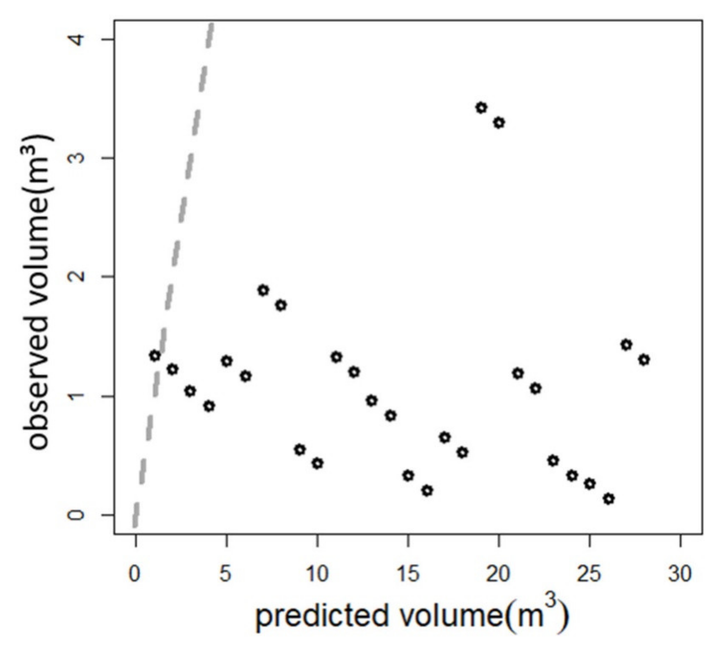
Our findings suggest that our approach may offer a viable improvement to utilizing maximum snow interception estimates based on LAI and CC. These metrics have been shown to be both inconsistently obtained and applied in hydrological models [2,9], and do not represent the three-dimensional spatial arrangement of canopy features associated with intrinsic baseline snow interception efficiency [11,12], whereas lidar-derived canopy metrics can be used to characterize complex structures, diverse age, and spatial variability. To illustrate the effectiveness of our model compared to the traditionally used LAI-based model, we first utilized the lidR package [58] to extract mean LAI values for each individual tree in our study area from the aerial lidar dataset. We then fit a generalized mixed-effects model in R with the lme4 package [59], predicting snow interception volume from LAI alone. This mixed-effects model with LAI as a fixed effect and tree ID as a random effect produced a marginal R2 = 0.01 (Figure 6), explaining considerably less variance than our random forests model incorporating several canopy metrics (R2 = 0.65).
Furthermore, our suggestion that predicting snow interception with canopy structural metrics may offer an improved approach to LAI-based estimates of snow interception employed in many hydrological models is consistent with the findings of Moeser and colleagues [33]. They found that novel ALS-derived metrics of canopy spacing (e.g., total gap area) were more highly correlated with snow interception than LAI. In future studies that utilize ALS data for estimating snow interception, we also suggest that researchers should consider combining canopy structural metrics, highlighted here as important predictors of snow interception volume, with canopy spacing metrics.
4.1. Variable Selection
Random forest modeling revealed that the nine most important canopy metrics for predicting intercepted snow volume (Figure 5) were measures of crown length and distribution on the stem (CL, CBH), tree and crown volume (ASV0.5, CV), unobstructed laser returns (UNOBDK), tree height (HRANGE, HSD, HMEAN), and crown surface area (CSA).
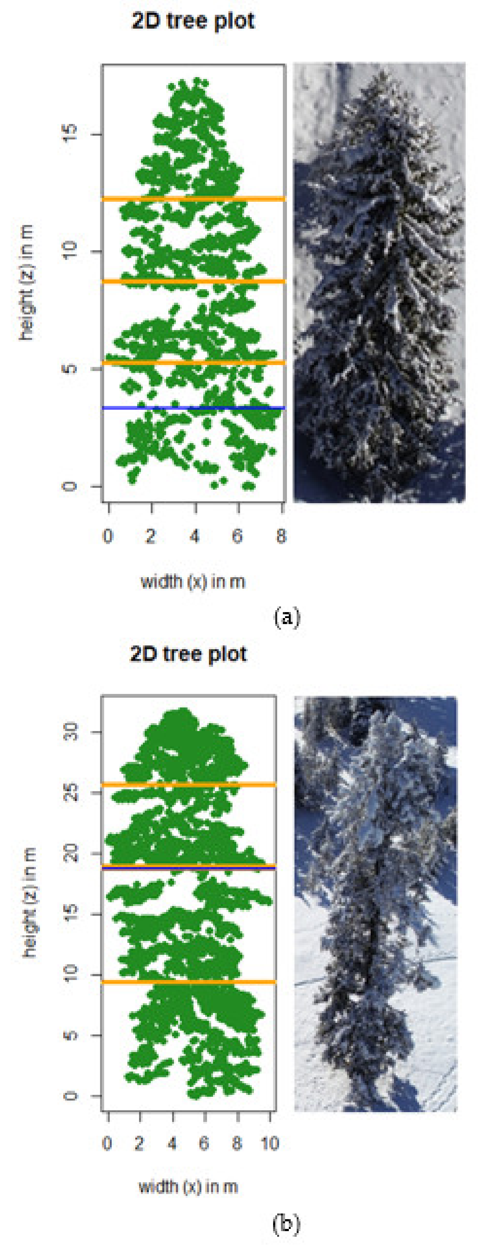
Crown length (CL) was ranked the most important variable, with a greater than 13% percent increase in the mean squared error when it was removed from the model (Figure 5). CL characterizes the portion of vegetative structure located above the crown base height. CBH was the fourth most important variable in our model, and is also an important biophysical parameter for many other applications in forest management, fuels treatment, wildfire modeling, etc. [60]. Our results suggest that variability in CBH, coupled with its correlation with other metrics (i.e., CL, CSA, CV), is an important factor in predicting the variability of canopy intercepted snow. Visual examination of our study trees reveals the relationship between CL, CBH, and the location of intercepted snow within each tree (Figure 7). For example, the tallest tree in our sample (tree #3; 31.7 m) intercepted 1.25 m3 of snow (averaged across December and January samples) with CBH = 18.7 m and CL = 13.0 m. Much of the canopy structure is in the upper 1/3 of the tree and visual inspection of the intercepted snow with unmanned aerial systems imagery (Figure 7a) shows most of the snow was captured by the uppermost crown. A shorter tree in our sample (tree #4; 17.3 m) averaged slightly higher intercepted snow (1.89 m3) with CBH = 3.3 m, CL = 14.0 m, and the canopy structure was more evenly distributed in the upper half of the tree (Figure 7b). This illustrates that the canopy distribution may partially control snow interception efficiency, but it also suggests that canopy metrics capture the idiosyncrasies of particular trees, as is the case with tree #3 (Figure 7, bottom left) in which some canopy structure clearly lies below the CBH and the fuller upper canopy. While the canopy distribution appears to be important, it must be acknowledged that wind speed and direction, and other extrinsic factors, may also be influential (Figure 1).
Whole-tree volume (ASV0.5) was ranked the second most important variable (Figure 5). This metric is an indicator of the overall structural potential for a tree to intercept snow anywhere along its stem. Examining the model performance in the context of individual trees, whereas whole tree volume of tree #3 (ASVO.5 = 42.90 m3) was significantly higher than that of tree #4 (ASVO.5 = 13.03 m3), it intercepted 0.64 m3 less snow (Figure 7). This suggests that different canopy structural metrics interact to affect snow interception, and that snow interception cannot be predicted as effectively with a simple linear regression model utilizing any individual metric. Indeed, such models do not perform as well as our random forest approach. For example, simple linear regressions fit with the two most important variables, CL and ASV0.5, generated much lower estimates of model fit (R2 ≤ 0.24) and higher estimates of model error (RMSE ≥ 0.60 m3). It should be noted that these simple linear regression models were fit separately for each sampling date to avoid temporal autocorrelation. Additionally, given the variable importance of whole-tree volume, it is possible that had not the lower 25% of TLS-derived samples been excluded due to occlusion from attached snowpack and ice, the ALS-derived canopy metrics may have even better explained the model variance. Excluding canopy metrics that corresponded to the lowermost returns (e.g., HMIN) was an attempt to align the TLS and ALS datasets, but this is a source of uncertainty that could not be avoided.
Finally, except under conditions of high wind, snow crystals deposit from a more or less vertical direction [48]. Hence, our novel metrics of unobstructed aerial lidar returns were especially well suited to characterize the vegetative structure that snow crystals first encounter when falling on to a tree. These metrics follow the principle that the first surfaces snow crystals encounter are the surfaces most likely to intercept and accumulate snow. While only one of our four novel metrics exceeded the 0.2 variable importance threshold, UNOBDK is the third most important metric (Figure 5). The importance of UNOBDK (versus UNOB) indicates that including an exponential decay function to account for some passage of snow below the first of overlapping returns is appropriate. This provides mechanistic evidence, given that some snow crystals may rebound and accumulate lower on the tree, or are later redistributed by wind and branch unloading [16].
4.2. Study Assumptions and Potential Sources of Error
We used TLS for model fitting. This remote sensing approach has been proposed as a viable direct sampling alternative [44] to traditional indirect sampling (e.g., forest/clearing comparisons in Moeser et al. [32,33]) or intensive controlled experimentation (e.g., weighing lysimeters in Storck et al. [5]). TLS-derived snow interception mass estimates have shown good agreement with snow interception estimates when compared against load cell measurements [44]. The TLS-derived snow volumes used in this study, however, should be viewed as relative rather than exact, measurements and they do not incorporate density estimates for the purpose of deriving snow water equivalent (SWE). In designing this study, we assumed that the processes of snow cohesion and bridging would fill interstitial spaces between branches and accumulate in new space beyond the original canopy profile, thereby counteracting potential TLS-based underestimation of snow volume due to branch deflection [16], gap creation through snow bridging [15], or occlusions in point clouds due to laser adsorption by snow [26,39,41] or laser scattering along the edges of the target [26,61]. Periodic reductions in tree volume with snow loading were observed though, suggesting that (although out of the scope for this study) further study is needed on (1) how snow loading affects whole-tree geometry of different species and trees subjected to variable temperatures, and (2) if, and to what magnitude, occlusions result from the interactions of laser energy and snow. To advance from estimating intercepted volume to intercepted SWE using our approach, we suggest that future studies characterize the snow densification process in canopies by, in part, improving on historic methods for capturing this data (e.g., [62]) and testing new techniques within the framework of a weighed tree experiment (e.g., [17]). Reliable in situ estimates of intercepted snow density could thus be combined with TLS-derived intercepted snow volume to produce SWE values for modeling.
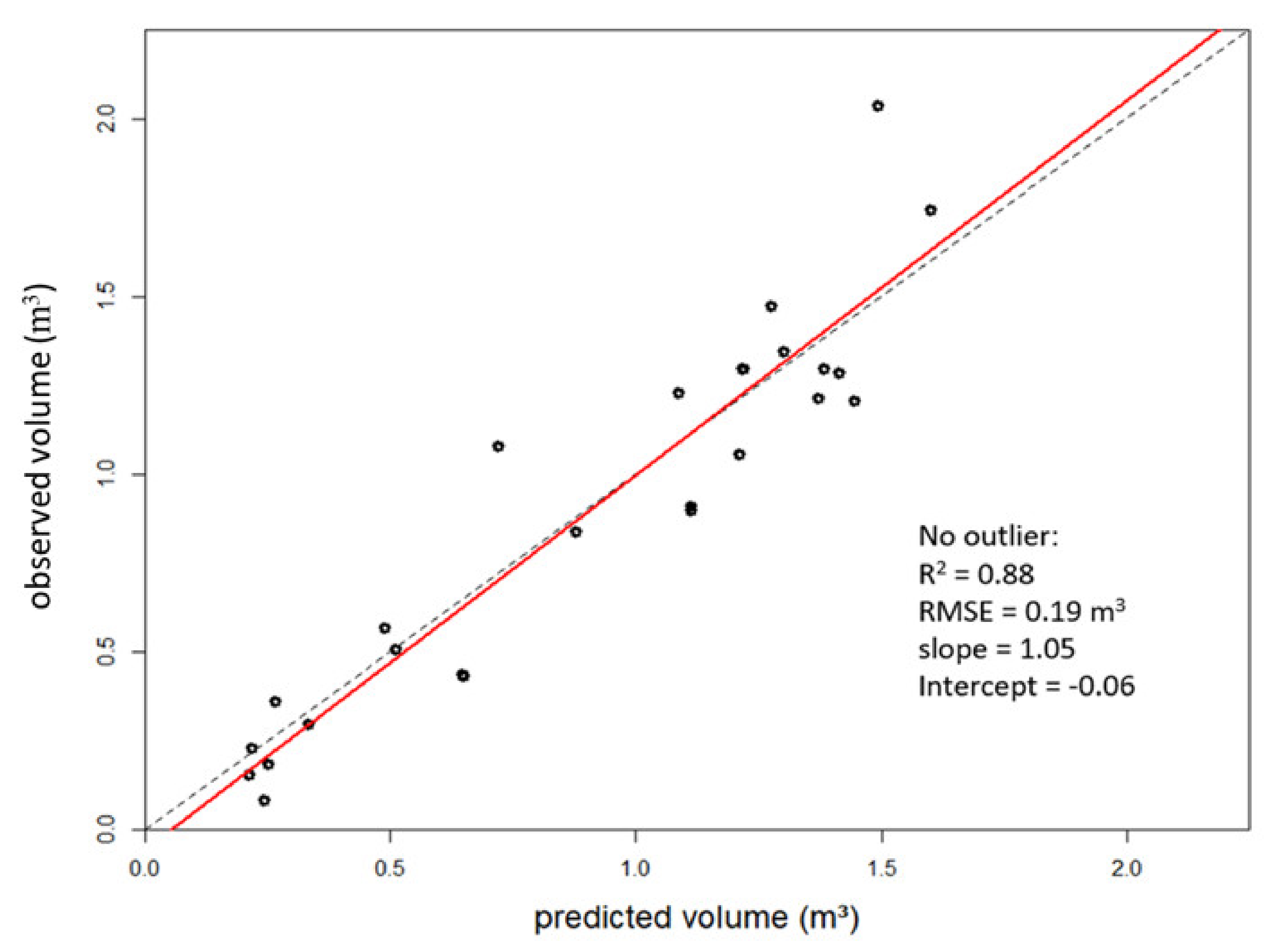
Model performance may have also been affected by the inclusion of outlier values associated with tree #10. Tree #10 is distinct from other individual-tree samples because it is a large dense clump of trees with several stems. This tree recorded the highest measured snow volume in both the December and January samples. Removal of these values from the final model increased model fit (R2 = 0.88; +0.22 compared to final model) and reduced model error (RMSE = 0.19 m3; −0.33 m3 compared to the final model) (Figure 8). These results imply that future research that applies our modeling approach to a larger area, particularly one with dense forest, may necessitate (1) calibration of individual tree detection algorithms that allow detection of individual trees from ATLS data (e.g., FindTreesCHM function in ‘rLiDAR’ package [46]), and (2) validation of how accurately these algorithms partition individual trees from clumps of trees (e.g., randomized visual inspection of ALS data or randomized field sampling). If there are limitations applying our modeling approach in dense forests due to challenges related to individual tree classification, or reduced canopy penetration by the laser beam (e.g., [63,64]), this may lend further credence to our suggestion that snow interception models include both canopy structural metrics and forest spacing metrics. Combining the two suites of intrinsic predictors, one suite providing data on individual trees and one suite providing data on canopy spacing, may reduce unexplained model variance by virtue of not relying on a single data type and its respective limitations.
5. Conclusions
The findings from this work suggest that ALS-derived canopy metrics can explain at least two-thirds of the variance in snow interception volume when extrinsic factors are held relatively constant. We also determined the specific suite of variables that generated the best fitting model, which included whole-tree volume, crown length, and weighted unobstructed returns. This study provides a potential improvement to parameterizing interception hydrological models based on metrics like LAI or canopy closure. Our approach is also increasingly more feasible given the wider availability of lidar data in complex forested terrain. Researchers interested in extending this work may look to understanding how well this approach performs across broader spatial extents encompassing a wider range of forest densities and may consider including both canopy metrics and forest spacing metrics in the intrinsic portion of snow interception models. Future researchers looking to expand the scope of this proof-of-concept study may also look to increase the sample size and incorporate more climatic data, thereby providing opportunities to explore the influence of local climate on snow interception and persistence of snow in the canopy.
Author Contributions
Conceptualization, M.R., J.U.H.E. and T.E.L.; methodology, M.R. and J.U.H.E.; software, M.R., J.U.H.E., and C.A.S.; validation, M.R. and J.U.H.E.; formal analysis, M.R. and J.U.H.E; investigation, M.R., J.U.H.E., and T.E.L.; data curation, M.R.; writing—original draft preparation, M.R.; writing—reviewing and editing, M.R., J.U.H.E., T.E.L. and C.A.S.; visualization, M.R. and J.U.H.E.; supervision, J.U.H.E.; project administration, J.U.H.E., funding acquisition, M.R. and J.U.H.E. All authors have read and agreed to the published version of the manuscript.
Funding
M.R. was supported by National Aeronautics and Space Administration Earth & Space Fellowship Program (18-EARTH18F-0208), the National Science Foundation Integrative Graduate Education and Research Traineeship Program (Award #1249400), and the Curt Berklund Graduate Research Scholar Fund. J.U.H.E. was supported by the NASA ABoVE grant NNX15AT86A. J.U.H.E. was further supported by the National Institute of Food and Agriculture, U.S. Department of Agriculture, McIntire Stennis project under 1018044.
Data Availability Statement
Russell, M.; Eitel, J.U.H., Link, T.E., Silva, C.A. Data from: Important airborne lidar metrics of canopy structure for estimating snow interception [Data set]. University of Idaho, 2021. https://0-doi-org.brum.beds.ac.uk/10.7923/3YXS-QK65 [65].
Acknowledgments
The authors wish to thank Arjan Meddens (Washington State University) for assistance with coding for Random Forests modeling, Andrew Maguire (NASA Jet Propulsion Laboratory) for review of an early draft and input on Random Forests modeling, and Ian Hellman (University of Idaho) for assistance with field work.
Conflicts of Interest
The authors declare no conflict of interest.
References
- Güntner, A.; Stuck, J.; Werth, S.; Döll, P.; Verzano, K.; Merz, B. A global analysis of temporal and spatial variations in continental water storage. Water Resour. Res. 2007, 43. [Google Scholar] [CrossRef]
- Rutter, N.; Essery, R.; Pomeroy, J.; Altimir, N.; Andreadis, K.; Baker, I.; Barr, A.; Bartlett, P.; Boone, A.; Deng, H.; et al. Evaluation of forest snow processes models (SnowMIP2). J. Geophys. Res. 2009, 114. [Google Scholar] [CrossRef] [Green Version]
- Varhola, A.; Coops, N.C.; Weiler, M.; Moore, R.D. Forest canopy effects on snow accumulation and ablation: An integrative review of empirical results. J. Hydrol. 2010, 392, 219–233. [Google Scholar] [CrossRef]
- Montesi, E.; Schmidt, D.; Montesi, J. Sublimation of Intercepted Snow within a Subalpine Forest Canopy at Two Elevations. J. Hydrometeorol. 2004, 5, 763–773. [Google Scholar] [CrossRef]
- Storck, P.; Lettenmaier, D.P.; Bolton, S.M. Measurement of snow interception and canopy effects on snow accumulation and melt in a mountainous maritime climate, Oregon, United States. Water Resour. Res. 2002, 38, 5-1–5-16. [Google Scholar] [CrossRef] [Green Version]
- Essery, R.; Pomeroy, J. Sublimation of snow intercepted by coniferous forest canopies in a climate model. IAHS-AISH Publ. 2001, 270, 343–347. [Google Scholar]
- Hedstrom, N.R.; Pomeroy, J.W. Measurements and modelling of snow interception in the boreal forest. Hydrol. Process. 1998, 12, 1611–1625. [Google Scholar] [CrossRef]
- Musselman, K.N.; Molotch, N.P.; Brooks, P.D.; Buttle, J.M.; Klein, A.G.; Pomeroy, J.W. Effects of vegetation on snow accumulation and ablation in a mid-latitude sub-alpine forest. Hydrol. Process. 2008, 22, 2767–2776. [Google Scholar] [CrossRef]
- Essery, R.; Rutter, N.; Pomeroy, J.; Baxter, R.; Stahli, M.; Gustafsson, D.; Barr, A.; Bartlett, P.; Elder, K. SNOWMIP2: An evaluation of forest snow process simulations. Bull. Am. Meteorol. Soc. 2009, 90, 1120–1135. [Google Scholar] [CrossRef] [Green Version]
- Pomeroy, J.W.; Gray, D.M.; Brown, T.; Hedstrom, N.R.; Quinton, W.L.; Granger, R.J.; Carey, S.K. The cold regions hydrological model: A platform for basing process representation and model structure on physical evidence. Hydrol. Process. 2007, 21, 2650–2667. [Google Scholar] [CrossRef]
- Kobayashi, D. Snow accumulation on a narrow board. Cold Reg. Sci. Technol. 1987, 13, 239–245. [Google Scholar] [CrossRef]
- Pfister, R.; Schneebeli, M. Snow accumulation on boards of different sizes and shapes. Hydrol. Process. 1999, 13, 2345–2355. [Google Scholar] [CrossRef]
- Schmidt, R.A.; Gluns, D.R. Snowfall interception on branches of three conifer species. Can. J. For. Res. 1991, 21, 1262–1269. [Google Scholar] [CrossRef]
- Brundl, M.; Bartelt, P.; Schneebeli, M.; Fluhler, H. Measuring branch defection of spruce branches caused by intercepted snow load. Hydrol. Process. 1999, 13, 2357–2369. [Google Scholar] [CrossRef]
- Satterlund, D.R.; Haupt, H.F. The disposition of snow caught by conifer crowns. Water Resour. Res. 1970, 6, 649–652. [Google Scholar] [CrossRef]
- Schmidt, R.; Pomeroy, J. Bending of a conifer branch at subfreezing temperatures: Implications for snow interception. Can. J. For. Res. 1990, 20, 1250–1253. [Google Scholar] [CrossRef]
- Martin, K.A.; Stan, J.T.; Dickerson-Lange, S.E.; Lutz, J.A.; Berman, J.W.; Gersonde, R.; Lundquist, J.D. Development and testing of a snow interceptometer to quantify canopy water storage and interception processes in the rain/snow transition zone of the North Cascades, Washington, USA. Water Resour. Res. 2013, 49, 3243–3256. [Google Scholar] [CrossRef]
- Roth, T.R.; Nolin, A.W. Characterizing maritime snow canopy interception in forested mountains. Water Resour. Res. 2019, 55, 4564–4581. [Google Scholar] [CrossRef]
- Hiemstra, C.A.; Liston, G.E.; Reiners, W.A. Snow Redistribution by Wind and Interactions with Vegetation at Upper Treeline in the Medicine Bow Mountains, Wyoming, U.S.A. Arct. Antarct. Alp. Res. 2002, 34, 262–273. [Google Scholar] [CrossRef]
- Webb, R.W.; Raleigh, M.S.; McGrath, D.; Molotch, N.P.; Elder, K.; Hiemstra, C. Within-stand boundary effects on snow water equivalent distribution in forested areas. Water Resour. Res. 2020, 56, e2019WR024905. [Google Scholar] [CrossRef]
- Bréda, N.J.J. Ground-based measurements of leaf area index: A review of methods, instruments and current controversies. J. Exp. Bot. 2003, 54, 2403–2417. [Google Scholar] [CrossRef]
- Song, C. Optical remote sensing of forest leaf area index and biomass. Prog. Phys. Geogr. 2013, 37, 98–113. [Google Scholar] [CrossRef]
- Bartlett, P.A.; MacKay, M.D.; Verseghy, V.D. Modified snow algorithms in the Canadian Land Surface Scheme: Model runs and sensitivity analysis at three boreal forest stands. Atmos.–Ocean 2006, 44, 207–222. [Google Scholar] [CrossRef]
- Friesen, J.; Lundquist, J.; Van Stan II, J.T. Evolution of forest precipitation water storage measurement methods. Hydrol. Process. 2015, 29, 2504–2520. [Google Scholar] [CrossRef]
- Eitel, J.U.; Vierling, L.A.; Magney, T.S. A lightweight, low cost autonomously operating terrestrial laser scanner for quantifying and monitoring ecosystem structural dynamics. Agric. For. Meteorol. 2013, 180, 86–96. [Google Scholar] [CrossRef]
- Deems, J.S.; Painter, T.H.; Finnegan, D.C. Lidar measurement of snow depth: A review. J. Glaciol. 2013, 59, 467–479. [Google Scholar] [CrossRef] [Green Version]
- Eitel, J.U.H.; Höfle, B.; Vierling, L.A.; Abellán, A.; Asner, G.P.; Deems, J.S.; Glennie, C.L.; Joerg, P.C.; LeWinter, A.L.; Magney, T.S.; et al. Beyond 3-D: The new spectrum of lidar applications for earth and ecological sciences. Remote Sens. Environ. 2016, 186, 372–392. [Google Scholar] [CrossRef] [Green Version]
- Timothy, D.; Onisimo, M.; Cletah, S.; Adelabu, S.; Tsitsi, B. Remote sensing of aboveground forest biomass: A review. Trop. Ecol. 2016, 57, 125–132. [Google Scholar]
- Wulder, M.A.; White, J.C.; Nelson, R.F.; Næsset, E.; Ørka, H.O.; Coops, N.C.; Hilker, T.; Bater, C.W.; Gobakken, T. Lidar sampling for large-area forest characterization: A review. Remote Sens. Environ. 2012, 121, 196–209. [Google Scholar] [CrossRef] [Green Version]
- Mazzotti, G.; Currier, W.R.; Deems, J.S.; Pflug, J.M.; Lundquist, J.D.; Jonas, T. Revisiting snow cover variability and canopy structure within forest stands: Insights from airborne lidar data. Water Resour. Res. 2019, 55, 6198–6216. [Google Scholar] [CrossRef]
- Zheng, Z.; Ma, Q.; Qian, K.; Bales, R.C. Canopy Effects on Snow Accumulation: Observations from Lidar, Canonical-View Photos, and Continuous Ground Measurements from Sensor Networks. Remote Sens. 2018, 10, 1769. [Google Scholar] [CrossRef] [Green Version]
- Moeser, D.; Stähli, M.; Jonas, T. Improved snow interception modeling using canopy parameters derived from airborne LiDAR data. Water Resour. Res. 2015, 51, 5041–5059. [Google Scholar] [CrossRef] [Green Version]
- Moeser, D.; Morsdorf, F.; Jonas, T. Novel forest structure metrics from airborne LiDAR data for improved snow interception estimation. Agric. For. Meteorol. 2015, 208, 40–49. [Google Scholar] [CrossRef]
- Lefsky, M.A.; Cohen, W.B.; Parker, G.G.; Harding, D.J. Lidar remote sensing for ecosystem studies: Lidar, an emerging remote sensing technology that directly measures the three-dimensional distribution of plant canopies, can accurately estimate vegetation structural attributes and should be of particular interest to forest, landscape, and global ecologists. BioScience 2002, 52, 19–30. [Google Scholar]
- Means, J.E.; Acker, S.A.; Fitt, B.J.; Renslow, M.; Emerson, L.; Hendrix, C.J. Predicting forest stand characteristics with airborne Lidar. Photogramm. Eng. Remote Sens. 2000, 66, 1367–1371. [Google Scholar]
- Coops, N.C.; Hilker, T.; Wulder, M.A.; St-Onge, B.; Newnham, G.; Siggins, A.; Trofymow, J.A. Estimating canopy structure of Douglas-fir forest stands from discrete-return LiDAR. Trees 2007, 21, 295–310. [Google Scholar] [CrossRef] [Green Version]
- Hilker, T.; Leeuwen, M.V.; Coops, N.C. Comparing canopy metrics derived from terrestrial and airborne laser scanning in a Douglas-fir dominated forest stand. Trees 2010, 24, 819–832. [Google Scholar] [CrossRef]
- Klauberg, C.; Hudak, A.T.; Silva, C.A.; Lewis, S.A.; Robichaud, P.R.; Jain, T.B. Characterizing fire effects on conifers at tree level from airborne laser scanning and high-resolution, multispectral satellite data. Ecol. Model. 2019, 412, 108820. [Google Scholar] [CrossRef]
- Prokop, A. Assessing the applicability of terrestrial laser scanning for spatial snow depth measurements. Cold Reg. Sci. Technol. 2008, 54, 155–163. [Google Scholar] [CrossRef]
- CloudCompare (version 2.10.2) GPL Software. 2017. Available online: http://www.cloudcompare.org/ (accessed on 11 November 2019).
- Kaasalainen, S.; Kaartinen, H.; Kukko, A. Snow cover change detection with laser scanning range and brightness measurements. EARSeL Eproc 2008, 7, 133–141. [Google Scholar]
- R Development Core Team. R: A Language and Environment for Statistical Computing; R Foundation for Statistical Computing: Vienna, Austria, 2013. [Google Scholar]
- Lafarge, T.; Pateiro-López, B.; Possolo, A.; Dunkers, J. R Implementation of a Polyhedral Approximation to a 3D Set of Points Using the Alpha-Shape. J. Stat. Softw. 2014, 56, 1–19. [Google Scholar] [CrossRef] [Green Version]
- Russell, M.; Eitel, J.H.; Maguire, A.J.; Link, T.E. Toward a novel laser-based approach for validating snow interception estimates. Remote Sens. 2020, 12, 1146. [Google Scholar] [CrossRef] [Green Version]
- USGS “The National Map”. 2019. Available online: https://viewer.nationalmap.gov/basic/ (accessed on 20 June 2019).
- Silva, C.; Crookston, N.; Hudak, A.; Vierling, L.; Klauberg, C. Package ‘rLiDAR’. 2015. Available online: https://cran.rproject.org/web/packages/rLiDAR/rLiDAR.pdf (accessed on 20 March 2021).
- Benaglia, T.; Chauveau, D.; Hunter, D.; Young, D. Mixtools: An R package for analyzing finite mixture models. J. Stat. Softw. 2009, 32, 1–29. [Google Scholar] [CrossRef] [Green Version]
- Miller, D.H. Res. Paper PSW-RP-18. In Interception Processes During Snowstorms; Pacific Southwest Forest & Range Experiment Station; Forest Service, US Department of Agriculture: Berkeley, CA, USA, 1964; Volume 18, pp. 18–43. [Google Scholar]
- Cutler, D.R.; Edwards, T.C., Jr.; Beard, K.H.; Cutler, A.; Hess, K.T.; Gibson, J.; Lawler, J. Random forests for classification in ecology. Ecology 2007, 88, 2783–2792. [Google Scholar] [CrossRef]
- Breiman, L. Random forests. Mach. Learn. 2001, 45, 5–32. [Google Scholar] [CrossRef] [Green Version]
- Belgiu, M.; Drăgu, L. Random forest in remote sensing: A review of applications and future directions. ISPRS J. Photogramm. Remote Sens. 2016, 114, 24–31. [Google Scholar] [CrossRef]
- Dormann, C.F.; Elith, J.; Bacher, S.; Buchmann, C.; Carl, G.; Carré, G.; Marquéz, J.R.G.; Gruber, B.; Lafourcade, B.; Leitão, P.J.; et al. Collinearity: A review of methods to deal with it and a simulation study evaluating their performance. Ecography 2013, 36, 027–046. [Google Scholar] [CrossRef]
- Liaw, A.; Wiener, M. Classification and Regression by randomForest. R News 2002, 2, 18–22. [Google Scholar]
- Genuer, R.; Poggi, J.M.; Tuleau-Malot, C. Variable selection using random forests. Pattern Recognit. Lett. 2010, 31, 2225–2236. [Google Scholar] [CrossRef] [Green Version]
- Strobl, C.; Boulesteix, A.L.; Zeileis, A.; Hothorn, T. Bias in random forest variable importance measures: Illustrations, sources and a solution. BMC Bioinf. 2007, 8, 25. [Google Scholar] [CrossRef] [Green Version]
- Millard, K.; Richardson, M. On the importance of training data sample selection in Random Forest image classification: A case study in peatland ecosystem mapping. Remote Sens. 2015, 7, 8489–8515. [Google Scholar] [CrossRef] [Green Version]
- Probst, P.; Janitza, S. Package ‘varImp’. 2019. Available online: https://cran.rproject.org/web/packages/varImp/varImp.pdf (accessed on 15 October 2019).
- Roussel, J.R.; Auty, D.; De Boisseu, F.; Meador, A.S.; Bourdon, J.F. Package ‘LidR’. 2018. Available online: https://cran.r-project.org/web/packages/lidR/lidR.pdf (accessed on 12 June 2019).
- Bates, D.; Mächler, M.; Bolker, B.; Walker, S. Fitting Linear Mixed-Effects Models Using lme4. J. Stat. Softw. 2015, 67, 1–48. [Google Scholar] [CrossRef]
- Luo, L.; Zhai, Q.; Su, Y.; Ma, Q.; Kelly, M.; Guo, Q. Simple method for direct crown base height estimation of individual conifer trees using airborne LiDAR data. Opt. Express 2018, 26, A562–A578. [Google Scholar] [CrossRef]
- Painter, T.H.; Dozier, J. Measurements of the hemispherical–directional reflectance of snow at fine spectral and angular resolution. J. Geophys. Res. 2004, 109, D18115. [Google Scholar] [CrossRef] [Green Version]
- United States. Army. Corps of Engineers. Snow Hydrology; Summary Report of the Snow Investigations; North Pacific Division, Corps of Engineers, U.S. Army: San Francisco, CA, USA, 1956. [Google Scholar]
- Broxton, P.D.; Harpold, A.A.; Biederman, J.A.; Troch, P.A.; Molotch, N.P.; Brooks, P.D. Quantifying the effects of vegetation structure on snow accumulation and ablation in mixed-conifer forests. Ecohydrology 2015, 8, 1073–1094. [Google Scholar] [CrossRef]
- Zheng, Z.; Kirchner, P.B.; Bales, R.C. Orographic and vegetation effects on snow accumulation in the southern Sierra Nevada: A statistical summary from LiDAR data. Cryosphere Discuss. 2015, 9, 4377–4405. [Google Scholar]
- Russell, M.; Eitel, J.U.H.; Link, T.E.; Silva, C.A. Data from: Important Airborne Lidar Metrics of Canopy Structure for Estimating Snow Interception [Data Set]; University of Idaho: Moscow, ID, USA, 2021. [Google Scholar] [CrossRef]
Figure 1.
Factors controlling snow interception efficiency.

Figure 2.
Study site location: Bear Basin Meadows, Payette National Forest, McCall Ranger District, Idaho.
Figure 2.
Study site location: Bear Basin Meadows, Payette National Forest, McCall Ranger District, Idaho.

Figure 3.
(a) Photo of the lead author conducting terrestrial laser scanning (TLS) at Bear Basin on December 5, 2018; (b) raw TLS point cloud data of two trees.
Figure 3.
(a) Photo of the lead author conducting terrestrial laser scanning (TLS) at Bear Basin on December 5, 2018; (b) raw TLS point cloud data of two trees.

Figure 4.
Predicted versus observed volume (m3) for the final random forest model. The dashed black line is the 1:1 line; the solid red line is the regression line.
Figure 4.
Predicted versus observed volume (m3) for the final random forest model. The dashed black line is the 1:1 line; the solid red line is the regression line.

Figure 5.
(a) Variable importance plot indicating the percent increase in mean squared error when each variable is removed from the model; (b) variable importance plot without percentiles.
Figure 5.
(a) Variable importance plot indicating the percent increase in mean squared error when each variable is removed from the model; (b) variable importance plot without percentiles.

Figure 6.
Predicted versus observed volume (m3) for the general mixed-effects model using LAI as the only predictor (marginal R2 = 0.01). Dashed grey line is the 1:1 line.
Figure 6.
Predicted versus observed volume (m3) for the general mixed-effects model using LAI as the only predictor (marginal R2 = 0.01). Dashed grey line is the 1:1 line.

Figure 7.
Two-dimensional tree plot of x and z coordinates with 25%, 50%, and 75% quartiles in orange and canopy length in light blue; unmanned aerial system image of corresponding trees from Dec. 5, 2018. Tree #3 (a) was 31.7 m and averaged 1.25 m3 intercepted snow volume; Tree #4 (b) was 17.3 m and averaged 1.89 m3 intercepted snow volume.

Figure 8.
Predicted versus observed volume (m3) for the final random forest model with no outlier included. Dashed black line is the 1:1 line; solid red line is the regression line.
Figure 8.
Predicted versus observed volume (m3) for the final random forest model with no outlier included. Dashed black line is the 1:1 line; solid red line is the regression line.


Table 1.
Standard ALS-derived tree crown metrics evaluated in this study. Novel metrics used in this study indicated with a ‘*’. Bold type indicates metrics included in the final simplified model.
Table 1.
Standard ALS-derived tree crown metrics evaluated in this study. Novel metrics used in this study indicated with a ‘*’. Bold type indicates metrics included in the final simplified model.
| Abbreviation | Definition |
|---|---|
| HMIN (m) | minimum crown height |
| HMAX (m) | maximum crown height |
| HMEAN (m) | mean crown height |
| HSD (m) | crown height standard deviation |
| HSKE | skewness of heights |
| HKUR | kurtosis of heights |
| HRANGE | HMAX-HMIN |
| HQR | interquartile range (H75TH–H25TH) |
| H25TH (m) | crown height 25th percentile |
| H50TH (m) | crown height 50th percentile |
| H75TH (m) | crown height 75th percentile |
| H90TH (m) | crown height 90th percentile |
| H95TH (m) | crown height 95th percentile |
| H99TH (m) | crown height 99th percentile |
| CL (m) | crown length (HMAX–CBH) |
| CBH (m) | crown base height (1.5 standard deviations below the height returns mean) |
| CRATIO | crown ratio (CL/HMAX) |
| CPA (m2) | crown area (π*CRAD2) |
| CV (m3) | crown volume as the convex hull 3D |
| CSA (m2) | crown surface area as the convex hull 3D |
| CDENS | percent crown density (returns ≥ CBH/total returns) |
| ASV0.25 | whole tree volume (α = 0.25) |
| ASV0.5 | whole tree volume (α = 0.50) |
| ASV0.75 | whole tree volume (α = 0.75) |
| UNOB | number of unobstructed returns * |
| UNOB% | percent unobstructed returns * |
| UNOBDK | number of unobstructed returns with decay function for weighted returns * |
| UNOBDK% | percent unobstructed returns with decay function for weighted returns * |
Publisher’s Note: MDPI stays neutral with regard to jurisdictional claims in published maps and institutional affiliations. |
© 2021 by the authors. Licensee MDPI, Basel, Switzerland. This article is an open access article distributed under the terms and conditions of the Creative Commons Attribution (CC BY) license (https://creativecommons.org/licenses/by/4.0/).
Share and Cite
MDPI and ACS Style
Russell, M.; Eitel, J.U.H.; Link, T.E.; Silva, C.A. Important Airborne Lidar Metrics of Canopy Structure for Estimating Snow Interception. Remote Sens. 2021, 13, 4188. https://0-doi-org.brum.beds.ac.uk/10.3390/rs13204188
AMA Style
Russell M, Eitel JUH, Link TE, Silva CA. Important Airborne Lidar Metrics of Canopy Structure for Estimating Snow Interception. Remote Sensing. 2021; 13(20):4188. https://0-doi-org.brum.beds.ac.uk/10.3390/rs13204188
Chicago/Turabian StyleRussell, Micah, Jan U. H. Eitel, Timothy E. Link, and Carlos A. Silva. 2021. "Important Airborne Lidar Metrics of Canopy Structure for Estimating Snow Interception" Remote Sensing 13, no. 20: 4188. https://0-doi-org.brum.beds.ac.uk/10.3390/rs13204188
Note that from the first issue of 2016, this journal uses article numbers instead of page numbers. See further details here.