Transferable Deep Learning from Time Series of Landsat Data for National Land-Cover Mapping with Noisy Labels: A Case Study of China

Abstract

Large-scale land-cover classification using a supervised algorithm is a challenging task. Enormous efforts have been made to manually process and check the production of national land-cover maps. This has led to complex pre- and post-processing and even the production of inaccurate mapping products from large-scale remote sensing images. Inspired by the recent success of deep learning techniques, in this study we provided a feasible automatic solution for improving the quality of national land-cover maps. However, the application of deep learning to national land-cover mapping remains limited because only small-scale noisy labels are available. To this end, a mutual transfer network MTNet was developed. MTNet is capable of learning better feature representations by mutually transferring pre-trained models from time-series of data and fine-tuning current data. An interactive training strategy such as this can effectively alleviate the effects of inaccurate or noisy labels and unbalanced sample distributions, thus yielding a relatively stable classification system. Extensive experiments were conducted by focusing on several representative regions to evaluate the classification results of our proposed method. Quantitative results showed that the proposed MTNet outperformed its baseline model about 1%, and the accuracy can be improved up to 6.45% compared with the model trained by the training set of another year. We also visualized the national classification maps generated by MTNet for two different time periods to quantitatively analyze the performance gain. It was concluded that the proposed MTNet provides an efficient method for large-scale land cover mapping.

1. Introduction

Large scale land-cover mapping is an important data source for monitoring changes in land cover and land use, managing land resources, and achieving sustainable development [1,2]. The most important factors affecting the accuracy of large scale land-cover maps are the model used for image classification and the training samples, which should provide sufficient information to train the model. Land-cover classification methods have developed from unsupervised to supervised methods. In the 1990s, clustering-based methods constituted the mainstream of land-cover mapping [3]. The spectral characteristics of objects are very complex to model, and this can result in unsatisfactory classification results [4]. Supervised methods, however, use samples of the detected classes to train a classifier and then use the trained classifier to predict the attributes of each pixel in a remote sensing image. With the help of the knowledge extracted from the training samples, supervised methods greatly outperform unsupervised ones [5].

The maximum likelihood classifier (MLC), the decision tree (DT), the random orest (RF) and the support vector machine (SVM) are the most popular supervised classifiers. The MLC uses statistical models to describe the characteristics of training samples [6,7]. It is suitable for application to images with known statistical distributions, but the data distribution needs to be assumed in advance. The essence of the DT is to build a set of rules that depend on the selected image features. The introduction of information gain gives it a chance to construct a diagram automatically and thus greatly expands its applications [8,9,10]. However, the classification results are still highly dependent on the selected image features and are sensitive to noise. The RF classifier was designed to overcome these drawbacks. The RF decreases the impact of image features by using an ensemble of DTs trained with various training sub-sets [11,12]. Sometimes, image features are difficult to distinguish in their original forms. Therefore, the SVM proposes to map the original image features to a higher- dimensional space in which the image features can be easily divided into two parts by a hyperplane [13,14]. A small number of support vectors are sufficient for estimating this hyperplane. However, in large-scale remote sensing images the same class presents different spectral features due to the difference of imaging conditions. A small number of training samples cannot cover all the image features of the same class. Thus, only using a small number of training samples to construct a classifier is a disadvantage in large-scale remote sensing image classification. A similar situation occurs in the other supervised classifiers mentioned above. To alleviate this drawback, a large-scale study area is often divided into several small sub-regions, and models in each sub-region are trained independently. However, this introduces another problem: the inconsistency in the classification criteria and the related accuracy between different sub-regions, which occurs even when complex pre- and post-processing is used.

A convolutional neural network (CNN) has the advantage of being able to learn essential features from a large set of training samples. Because of this, CNN has achieved great success in computer vision. This gives us a reference in large-scale remote sensing land-cover mapping, which has attracted a significant amount of attention [15,16]. Most of these networks end up with fully connected layers. These kinds of networks assume that all pixels in an image patch share the same label and that only the center pixel label can be predicted each time. This not only seriously affects the efficiency of large-scale products but also leads to inaccurate segmentation results, especially near the boundary of objects when the input image patch contains more than one class. Fully convolutional networks are only composed of convolutional layers. Networks such as these output the labels of all the pixels in the input image and can thus avoid the drawbacks of patch-based ones. FCN was the first fully convolutional network; this extracts information from the input image using a range of convolutional kernels [17]. However, detailed information about the detected objects may be lost during the stacking of convolutional and pooling layers, and the object boundaries in FCN are unsatisfactory. Unet adopts a hierarchical upsampling strategy to reconstruct target details and concatenates upsampled layers into corresponding downsampled ones to improve the transfer efficiency for the detailed information [18]. However, the contribution of detailed information and small object features to the final classification results is small as only low-level features are concatenated with high-level ones. PSPNet uses multiple branches to extract a range of information and then downsamples the learned information to different scales to construct dependencies at different scales [19]. By concatenating features at different scales, PSPNet is able to learn both the global information and detailed information. Considering the scales of objects captured in large-scale remote sensing images, PSPNet is suitable for the corresponding land cover mapping. Unfortunately, CNN-based models need a large amount of accurately annotated training samples.

Enough high-quality training samples for large-scale land-cover mapping are difficult to access to [20]. Insufficient or unreliable training samples may cause serious misclassification [21,22]. Manual labeling is labor intensive and error-prone. Traditional image classification algorithms use point-based samples to train the classifier, and the training samples can be obtained by automatic sample selection methods according to their radiometric information or other characteristics [23]. On the contrary, samples for CNN should be labeled pixel-wise, which makes it much more difficult to access. Existing high-precision land-cover maps have high-potential sample resource value. When constructing training sets from existing land-cover maps, the most serious problem is a noisy label (a label that does not represent the real label of the corresponding pixel).

Traditional data-cleaning methods cannot be directly used on pixel-wise training samples [24]. Other methods such as noise transition and relabeling may need human assistance, which makes them tedious and error-prone [25,26,27]. Using specially defined loss functions and corresponding reweighing methods needs enough knowledge about the training set, which is a huge workload for large-scale land cover mapping [28,29]. Existing small-scale noisy labels contain enough information, which can be used for large-scale land cover mapping if properly used. Fortunately, time series images contain complementary information due to the difference in time series imaging conditions. Aiming at fully utilizing the information in original Landsat images to overcome the drawbacks of noisy labels, we proposed the use of a mutual transfer network (MTNet) by using the transferring property of CNNs. The model trained in one year was considered as a good initialization and also a regularization on the target training samples to improve the generality of the networks. In this study, PSPNet was employed as the baseline due to its local and global information extraction ability and the changes in object scale in the remote sensing image. The main contributions can be summarized as follows.

(1)

To the best of our knowledge, this is the first time that a mutual deep-learning model of this type—that is, a MTNet that can be used for national-level land cover mapping—has been developed.

(2)

A novel interactive training strategy was proposed, and this was embedded into our MTNet to produce large-scale land cover maps with unbalanced training samples and noisy labels.

(3)

Extensive experiments conducted on national land-cover datasets for 2005 and 2010 demonstrated the effectiveness and superiority of the proposed MTNet, yielding national land-cover maps with high accuracy.

The remainder of this article is arranged as follows. First, previous studies are introduced in Section 2. The data sources and corresponding training sets are shown in Section 3. Then, the proposed MTNet is described in detail in Section 4. Experiments for two different time periods (2005 and 2010) are carried out to test the effectiveness of the proposed MTNet in Section 5. Then, the experiments are extended to the national level to achieve highly accurate land cover maps of China in Section 6. Conclusions and ideas for future work are discussed in Section 7.

2. Previous Studies

2.1. CNN-Based Land-Cover Mapping

The rise of convolutional neural networks (CNNs) in computer vision has provided a new concept that can be used in large-scale land-cover mapping due to its advantages in processing big data. Rezaee et al. [30] used AlexNet [31] to extract areas of wetland from remote sensing images, and it was found that this method outperformed traditional classifiers. To improve the diversity of learned feature maps, Huang combined AlexNet with a light parallel network [32] and achieved a classification accuracy of up to 80%. However, training a network requires a large number of accurate training samples, and these are usually difficult to access in the context of remote sensing imagery. The network was fine-tuned using pre-trained models in ImageNet, and the overall accuracy improved from 83.1% to 92.4% [33]. Besides pre-trained models, image augmentation has also been demonstrated to produce more efficient remote sensing image classification [34].

The CNNs that were mentioned above all end up with fully-connected layers, which means that they assume pixels from the image batch share the same label and predict the label of middle pixels instead of the whole image batch. This assumption leads to inaccurate classification results near target boundaries. To reduce this phenomenon, superpixel- and object-based networks have been developed [35,36]. The consistent spectrum information provided by superpixels is able to improve the recognition ability of CNNs [37]. However, the application of CNNs to large-scale land-cover mapping still face problems such as weak generalization, rotation variance and the difficulty of collecting pixel-level training samples. To solve these problems, pooling layers were recombined to improve the efficiency of information transmission in the network, and hierarchical sampling strategies were proposed to automatically construct training datasets [38]. The rotation equivalence was encoded in a CNN architecture to maintain the rotation invariance [39].

Most traditional classifiers utilize image features with clear physical meanings. These features are easy to understand and can provide stable information for classifiers. On the contrary, the feature maps in CNNs are learned from the training samples automatically, which makes it incomprehensible. To make full use of the difference in their features, a decision-based classifier that was able to combine the features from RF, SVM and CNNs was designed [40]. As well as the features learned by traditional classifiers and CNNs, the feature maps learned by CNNs were also different [41]. The use of ensemble CNNs is also an efficient method of improving the classification performance [42]. Ref. [43] combined contextual-based CNNs with pixel-based multilayer perceptron (MLP) to take advantage of both the spatial and spectral feature representations. To further explore the advantages of CNNs and MLP, Ref. [44] proposed a joint learning strategy that learned the joint distribution between CNN and MLP. The proposed algorithm was demonstrated to produce a great increase in the classification accuracy.

2.2. Noisy Label Problem

A noisy label is an inevitable problem in the practice of land cover mapping. For traditional classifiers, which use point-based training samples, detecting and filtering noisy labels is an effective method [45,46]. However, it is invalid in pixel-wise-labeled samples for CNN. Fortunately, the effects of a noisy label and a correct label on the learning process are different [47]. To fully utilize this property, Ref. [46] used a self-organizing map to identify inliers and outliers. Ref. [48] proposed to exploit model consistency across iterations and combined a hard mask selection and soft mask reweighing to invalid noisy labels without discarding possibly clean ones. In fact, outliers also contain usefully information, so identifying and discarding them will be fatal, especially when training samples are insufficient. To overcome this drawback, Ref. [49] proposed to use the uncertainty information of training samples and proposed an uncertain aware co-training method to achieve good generalization performance. Ref. [50] proposed a turning value to effectively learn positive samples over negative ones to increase the learning ability of the network. However, it is difficult to recognize and evaluate correct labels and noisy labels. Ref. [45] randomly selected some seed points as clean labels and propagated the label information from them to the rest unlabeled samples. Ref. [51] proposed a coarse-to-fine label iteration model to dig out a set of high-quality labels from fully aggregated labels by using a sparse filter.

The loss function dominates the learning preference of deep learning networks. Different loss functions focus on describing different aspects of the difference between the predicted result and the corresponding label. For most of the loss functions, it is a robust to noisy label to some extent in the presence of a large amount of training samples. However, too many noisy labels will affect the generality of the network [52]. Ref. [53] combined mix-up entropy and Kullback–Leibler entropy to define a new loss function by fully utilizing the difference between them. A similar idea was performed in [54]. Ref. [55] proposed an end-to-end correction with mix-up and balance terms to correct noisy labels to true labels. To fully utilize the similarities of pixels belonging to the same class, Ref. [56] proposed a dubbed self-reweighing from the class centroids method. The class centroids can be used to measure the reliability of data labels and thus improve the robustness to noisy labels. Besides the loss function, the structure of the CNN network also has a great impact on its learning ability. Ref. [54] proposed a novel dual-channel structure to improve the learning ability along with a noisy robust loss function constructed by reverse cross entropy and normalized cross entropy.

3. Data Description

3.1. Data Sources

For large-scale land cover mapping, data availability and corresponding observation ability are the main factors affecting the selection of data sources. Although full-wave LiDAR contain back scattering information about the detected object, it is still difficult to recognize the detected classes. In addition, LiDAR implies the highest cost among commonly used remote sensing datasets [56,57]. SAR is a cost-effective alternative to LiDAR and is unaffected by clouds. However, the back scattering and interferometric coherence in special areas are serious, leading to unclear structure representation [58]. Overall, optical images are the most appropriate even though it is easily affected by clouds. As for the observation ability, low-resolution images cannot reflect the detailed information about the detected objects, which will affect the distinguishing ability on different classes, such as vegetation type. Intermediate-resolution Landsat and Sentinel images are the most commonly used resources in large-scale land cover mapping. Experiments demonstrated that even though Sentinel images have a higher spatial resolution, the overall accuracy of land cover maps produced by Landsat 8 images is similar to that produced by Sentinel-2 images [59]. Considering the long time series, Landsat images were employed in this work. The Level 1T Landsat 5 images of the years 2005 and 2010 from growing seasons were downloaded from https://earthexplorer.usgs.gov (accessed on 10 December 2017).

Different from traditional classifiers, pixel-wise-labeled image patches are necessary to train a fully convolutional neural network. That means most of the existing training samples are invalid for CNN. Manually labeling samples for CNN is labor-intensive and, more importantly, unreliable. Under this circumstance, existing high-accuracy land cover maps can be an option. The Land Cover Map of the People’s Republic of China is a high accuracy time series product, which is widely accepted. It can be downloaded from http://www.geodata.cn (accessed on 10 April 2018). This map contains six first-level classes and 38 second-level classes (details shown in

Table 1. Relationship between the proposed 8 first-level classes and the 38 second-level classes in the reference.

First-Level Classes	Second-Level Classes
Forest	Evergreen broad-leaved forest, deciduous broad-leaved forest, evergreen needle-leaved forest, deciduous needle-leaved forest,
	Mixed-leaved forest, evergreen broad-leaved shrub, deciduous broad-leaved shrub, evergreen needle-leaved shrub, arbor garden,
	Shrub garden, arbor green space, shrub field
Grassland	meadow, grassland, grass, herbaceous green land
Wetland	Forest wetland, shrub wetland, herbal wetland
Water body	Lakes, reservoirs/ponds, rivers, canals
Cultivated land	Irrigated farmland, farmland
Artificial surface	Residential land, industrial land, transportation land
Bare land	Mining land, sparse forest, sparse shrub, sparse grassland, moss/lichen, bare rock, bare soil, desert/sandy land, saline-alkali land
Snow and ice	Glacier/permanent snow cover

) that have overall accuracies of 94% and 86%, respectively.

3.2. Data Pre-Processing

Pre-processing is inevitable in traditional large-scale land cover mapping, since it can provide reliable back-scattering properties of the detected classes. However, the laborious and time-consuming pre-processing heavily affects the practical application in large-scale land cover mapping. Fortunately, CNNs use a large number of parameters to approximate the transformation from input image to output labels, and they are robust to the changes in spectral features in large-scale remote sensing images. That makes it a natural choice for large-scale land cover mapping, which can avoid laborious pre-processing such as radiometric calibration and atmospheric correction. For convenience of automatic processing, an image mosaic using median values was performed to alleviate the impact of clouds, images from non-vegetation season, etc. As for the reference, the data downloaded from http://www.geodata.cn (accessed on 10 April 2018) were stored in provinces. It can be directly aligned with the mosaicked Landsat images. However, to fully utilize the label information, its classification system should be modified to adapt the representation ability of Landsat images. Referencing existing classification systems employed in [60] and other commonly accepted land-cover maps, the 38 second-level classes were merged into 8 first-level classes, as shown in Table 1. Then, the merged land cover map was considered as a reference.

3.3. Study Area and Training Sets

In the sample selection stage, the sample distribution and the accuracy of the corresponding reference had the most impact on the construction of the training sets. Therefore, the selected samples should be evenly distributed and should avoid the location of obvious classification errors. For training CNN, the larger the sample size is, the more information it contains, and yet, more computation is needed.The larger the size of a training sample, the more global features it can represent; however, more GPU memory is also required. To make a trade-off between the expression of global characteristics and the computation ability of the GPU, a $512\times 512$ pixel size was chosen. For the experiments in this study, 80% of the selected samples constructed the training set, and the other 20% acted as the validation set.

3.3.1. Training Samples for the Jing-Jin-Ji Region with Different Composition

It is known that the quality and quantity of training samples has a great impact on the accuracy of supervised classifiers [61]. For most large-scale land cover mapping training sets, there is a significant amount of redundant information contained, as well as inaccurate information. Experiments in [62] demonstrated that the RF classifier can achieve stable global land cover maps even with 60% fewer sample points or containing 20% errors from the whole training set, which contain 340,000 sample units of various sizes (from 30 m × 30 m to 500 m × 500 m) located at approximately 93,000 sites worldwide. However, the training samples used in this study were pixel-wise image patches, which were cropped from existing classification results and matched with the collected original Landsat images. That means we could not accurately evaluate the accuracy of training samples without a great effort. Therefore, we designed a small experiment to reflect the accuracy of the training samples. In this experiment, the Jing-Jin-Ji region as shown in Figure 1 was selected due to the rich classes contained in this region.

Impacted by the change in coverage with the seasons and years, as well as the similarity of spectral features of vegetation types, there exist obvious labeling errors among vegetation types in the training set. Hence, three training sets were constructed in the Jing-Jin-Ji region to reflect the accuracy objectively.

• TS-1: This set consisted of 1280 training samples covering all the classes present in the study area, namely, forest, grassland, wetland, water body, cultivated land, artificial surface and bare land.
• TS-2: As there exists serious confusion in the labels of grassland and forest in TS-1, these two classes were merged to decrease the impact of labeling errors in this set.
• TS-3: In this set, the grassland was oversampled so that the impact of the proportion of inaccurate classes on the final land-cover map could be explored.

3.3.2. Typical Regions

The Chinese provinces of Liaoning, Hubei and Qinghai were selected as study areas. The locations of these areas within China are shown in Figure 2, in which the original Landsat images are represented in pseudo-color composed by NIR, red and green bands. Liaoning is located in northeast China and is mainly composed of cultivated land, artificial surfaces, forest and grassland. Affected by the low temperature, the vegetation types of the same class are obviously different from other regions, leading to different spectral features in vegetation type. Hubei is located in the middle of China. There are thousands of lakes in this province, so it is a perfect study area to test the accuracy of the classification on water bodies. Qinghai province is located on the Qinghai–Tibet Plateau, very far away from the sea. This province is mainly composed of bare land and grassland; in addition, 15.19% of wetlands in China are found in this province. Similar to the experiments on the Jing-Jin-Ji region, the labels shown in Figure 2 were taken from the reference derived from Land Cover Map of the People’s Republic of China.

Considering the influence of proportions in the training set, 15,000 non-overlapping samples with $512\times 512$ pixels from across China were collected for 2005 and 2010 except for the three provinces that had been selected as study areas. Four thousand samples with $512\times 512$ pixels were selected from the study areas and used for validation (as shown in

Table 2. Details for the training sets.

	Training Samples	Test Samples	Patch Size	Channels
Typical region	15,000	4000	512 $\times 512$	6
Whole nation	19,200	4800	$512\times 512$	6

). There were significant differences in the quantity of the training samples for each class due to the natural imbalance between these classes within China. Besides, original Landsat images for 2005 contained some images obtained from the non-growing season, which increased the uncertainty in its samples. To express different features as comprehensively as possible, the selected samples contained different spectral features that expressed the same objects in different locations. Additionally, the training set contained objects with different sizes to make it possible for the DL-based method to learn both detailed and global information. All six bands except the thermal infrared were used to provide sufficient information for the classifier.

3.3.3. The Whole Nation of China

As discussed in Section 3.1, 1056 Landsat 5 images with Level 1T from the growing seasons of the years 2005 and 2010 were collected. The pre-processed images (mosaicked) are shown in Figure 3. The stitching lines between the image tiles are obvious: this is caused by the variation in the spectral values in different images. Comparing the original images of China for 2005 and 2010, the vegetation cover in 2005 was lower than that in 2010, especially in the regions circled in blue. Figure 3a contains more images from outside the growing seasons. However, the labels for these regions were obtained during the growing seasons.

To train a network that could be used in national-land cover mapping, for both 2005 and 2010, 19200 non-overlapping training samples were manually selected, each with a size of $512\times 512$ pixels as shown in Table 2. The two training sets from typical regions and the whole nation were composed of two time periods, namely, 2005 and 2010. Time series training samples were employed to increase the generality of the proposed MTNet in this study, due to the similarity between their image features and the difference of the corresponding information. Since we wanted to train a network that would be used to produce a national land-cover map of China, the selected training samples were distributed across the whole nation. More training samples were taken from regions where more features were presented, such as eastern coastal areas; fewer training samples were acquired from regions containing fewer features, such as the large areas of grassland and desert with China. It is well known that the learning ability of the DL network is better when the training samples are balanced. If a DL-based network is used with an unbalanced training set, the accuracy of the classes that occupies a small proportion tends to be sacrificed to ensure the overall accuracy. However, the distribution of classes across China as a whole is naturally unbalanced. Considering the influence of different proportions of each class, the proportion of the less distributed classes are increased to match the proportion of majority classes to balance the training set as much as possible. The proportions of different classes for the whole of China and in the training set are shown in Figure 4. Less-distributed classes such as water bodies, artificial surfaces and snow and ice clearly had greater proportions in the training set than their actual proportions within China; for wetland, the opposite was the case. The reason for this is that the areas of wetland were very dispersed, and this made it difficult to collect training samples for this class. Even if a greater effort had been made to achieve a better balance between the class proportions, the variation would still have been large.

4. Methodology

Traditional CNNs learn essential features from a training set, in which sufficient high-quality training samples are necessary. However, sufficient high-quality training samples are difficult to access, especially for large-scale study areas. Fortunately, small-scale noisy labels can be derived from existing land cover maps. Although CNN is robust to noise to some extent, the learning ability is highly dependent on the degree of noise corruption. Serious noise corruption will lead the network to over-fitting, which will seriously decrease the quality of the reduced land cover mapping. As a widely used source for land cover mapping, Landsat images are superior to other remote sensing images in terms of long-term and stable observation ability. The similarity and difference information contained in time series Landsat image gave us a chance to overcome the drawback brought by inaccurate training samples by providing various features for the same class and thus improving the generality of the network. To fully utilize the consistency and complementarity of time series images, a mutual transfer network called MTNet was proposed in this study. First, the DL-based network was trained by the time series training set introduced in Section 3. As the training samples in the time series are similar, the purpose of this step in the training process was to learn the essential features of the training samples: the more details that can be learned, the better. Then, the trained network was used as an initialization on the current training set. Benefiting from the consistency of Landsat images, the fine-tuned process on current data cannot only make full use of the learned essential information but can also adapt to the distribution of the current classes. In addition, the initially trained MTNet can be considered as a regularization on the time series training set to resist the impact of noisy labels and thus improve the generality of the network.

CNN stacks convolutional layers to extract information from input images. The convolutional layer can be expressed as

$$X^{(t+1)}=f\left(w^{\left(t\right)}{X}^{\left(t\right)}+b^{\left(t\right)}\right)$$

(1)

where t represents the iteration index; $X^{\left(t\right)}$ is the input image; $w^{\left(t\right)}$ is the parameter of the convolutional kernel, which slides over $X^{\left(t\right)}$; $b^{\left(t\right)}$ is the bias of the learned features and $f(·)$ is an activation function that can convert a linear combination of information into a non-linear one. By stacking different convolutional kernels, the same classes present similar features, while different classes present different features. The learned features were mainly dominated by the training process. Taking the Adam optimizer as an example, the gradient, the first-order momentum and the second-order momentum can be calculated as

$$\begin{array}{cc}\hfill & g^{\left(t\right)}={\nabla }_{w}f\left(w^{\left(t\right)}\right)\hfill \\ \hfill & m^{\left(t\right)}={\beta }_1{m}^{(t-1)}+(1-{\beta }_1)g^{\left(t\right)}\hfill \\ \hfill & V^{\left(t\right)}={\beta }_2{V}^{(t-1)}+(1-{\beta }_2){\left(g^{\left(t\right)}\right)}^2\hfill \end{array}$$

(2)

Here, ${\beta }_1$ and ${\beta }_2$ are coefficients of the first- and second-order momentum, respectively. The step is then given by

$${\eta }^{\left(t\right)}=\alpha \frac{m^{\left(t\right)}}{\sqrt{V^{\left(t\right)}}}$$

(3)

Finally, the updated $w^{\left(t\right)}$ is given by

$$w^{(t+1)}=w^{\left(t\right)}-{\eta }^{\left(t\right)}$$

(4)

When the training set is imbalanced or contains noisy labels, the calculation of Equations (2) and (3) will have large deviations, thus leading to over fitting. On the contrary, time series training samples can provide additive information and generalize the distribution of the classes. Due to the increase in correctly labeled samples in the generalized distribution, it is more robust to imbalanced and noisy labels. To take advantage of this property, an MTNet was proposed. Firstly, the proposed MTNet trained the network with one of the time series training sets to approach the optimum parameters. Then, the trained model was used as an initialization to fine-tune the model on the current data. As an initialization, it can provide a near-optimum combination of parameters. On this basis, the fine-tuned network can not only converge faster but also better adapt to the distribution of the target domain. In this way, Equation (4) was obtained by two training sets: the original parameter $w^{\left(t\right)}$ comes from the time series training set, which was used to train the MTNet, and the gradient ${\eta }^{\left(t\right)}$, which was obtained from the current training set to further approach the optimum. The disagreements between the time series training sets are the main source of information in the mutual learning. The learned parameters can be written in the form

$$w_{final}=w_{first\_set}+w_{second\_set}$$

(5)

where $w_{first\_set}$ represents the parameters trained by the time series training set that dominates the learning ability of the MTNet; $\Delta w_{second\_set}$ represents the updated parameters, which were fine-tuned on the current training set. As a regularization, the pre-trained model can provide diversified information to enlarge the parameter space. In counter with the training process, which reduces the searching scope of the parameter space, the pre-trained model can prevent the network from learning features that are too complex. In other words, by utilizing the consistency and complementarity between time series Landsat images, the MTNet is able to prevent the network from over-fitting in the presence of noisy labels.

Taking PSPNet as an example, the flowchart of the proposed MTNet is shown in Figure 5. The efficiency of the MTNet is improved by ensuring that the network learns essential and general features from time series training sets. By fully utilizing the similar and dissimilar features of the time series training sets, the MTNet can learn general information and is also robust to imbalanced and noisy labels.

5. Experiments and Analysis on Typical Regions

The network was coded using Pytorch and trained by a 3 Titan XP with a 12 GB memory. To improve the efficiency and decrease the number of training samples needed, a model that had been pre-trained on ImageNet was employed to initialize the network parameters. An Adam optimizer was used to calculate the gradient of the network and realize the backward propagation. The learning rate was set to ${10}^{-4}$, and the weight decay was ${10}^{-4}$. The batch size was 18 with a momentum of 0.1. The network was trained 300 epochs and fine-tuned 40 epochs so that it could fully utilize the information contained in the time series images.

5.1. Experiments on Different Compositions of Training Samples

PSPNet was used to classify the above-mentioned three training sets in Section 3.3.1. The corresponding precisions are listed in

Table 3. Classification accuracy for the Jing-Jin-Ji region of PSPNet on the four training sets where forest and grassland are merged as on class in TS-2.

	Forest		Grassland		Wetland		Water Body		Cultivated Land		Build-Up Land		Bare Land		Overall Accuracy
(%)	Precision	F1_Score	Precision	F1_Score	Precision	F1_Score	Precision	F1_Score	Precision	F1_Score	Precision	F1_Score	Precision	F1_Score	Precision	F1_Score
TS-1	81.54	76.34	36.05	49.80	41.82	57.23	71.66	16.89	90.34	81.79	47.50	58.61	37.73	49.63	75.25	71.83
TS-2	87.61 78.94				48.43	60.17	72.48	29.11	85.05	83.22	56.49	76.20	41.90	38.90	83.16	78.32
TS-3	81.74	77.16	54.61	56.99	49.60	63.21	75.39	34.11	87.17	78.45	58.11	63.92	45.98	49.40	77.65	72.43

. Comparing the classification results of TS-2 with TS-1, it was clear that combining the labels of forest and grassland can significantly improve both the precision (from 75.25% to 83.16%) and the F1_score (from 71.83% to 78.32%). Of course, merging classes simplifies the learning model, but the improvement in the accuracy of the training set also contributes to the improvement in the precision and the F1_score. The existence of labeling errors in the training set cannot only affect the recognition of the corresponding class but also improves the learning ability of the network. Actually, the quality of the training set cannot be easily improved in real-world tasks. So, it is difficult to quantitatively describe the connection between the noisy corruption degree and the learning ability of the network.

As for the classification result of TS-3, increasing the proportion of grassland also increases the proportion of forest, since they usually appear to be adjacent. With more information about grassland, the classification precision rose about 18.56%, and the F1_score increased about 7.11%. Similar to the result of TS-2, all the other classes except cultivated land were all increased in TS-3. This means that introducing more information can significantly increase the learning ability of CNN, even though the introduced information was with uncertainty. That gave us a clue to jointly learn from time series remote sensing images by using the similar but differential information.

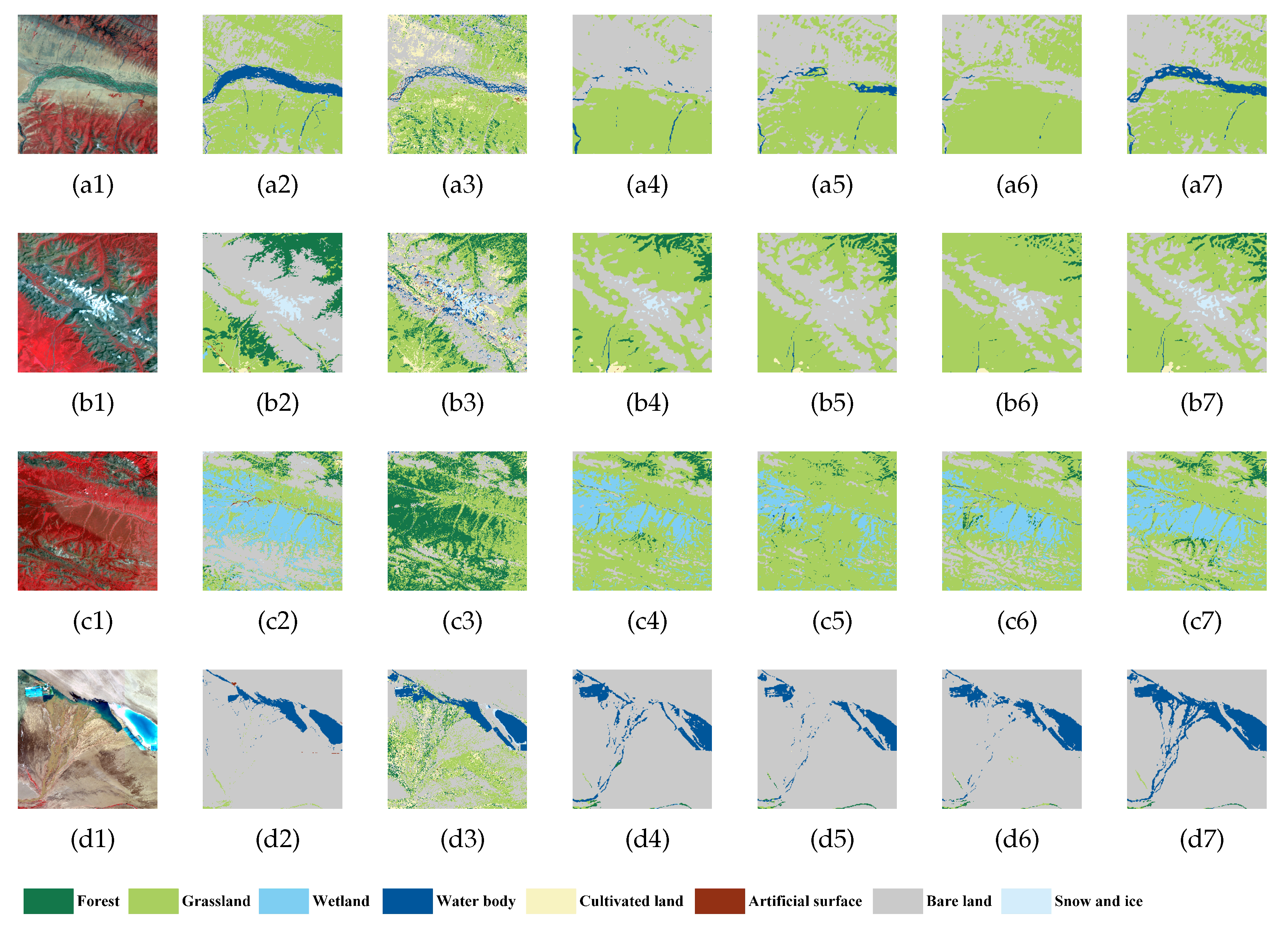
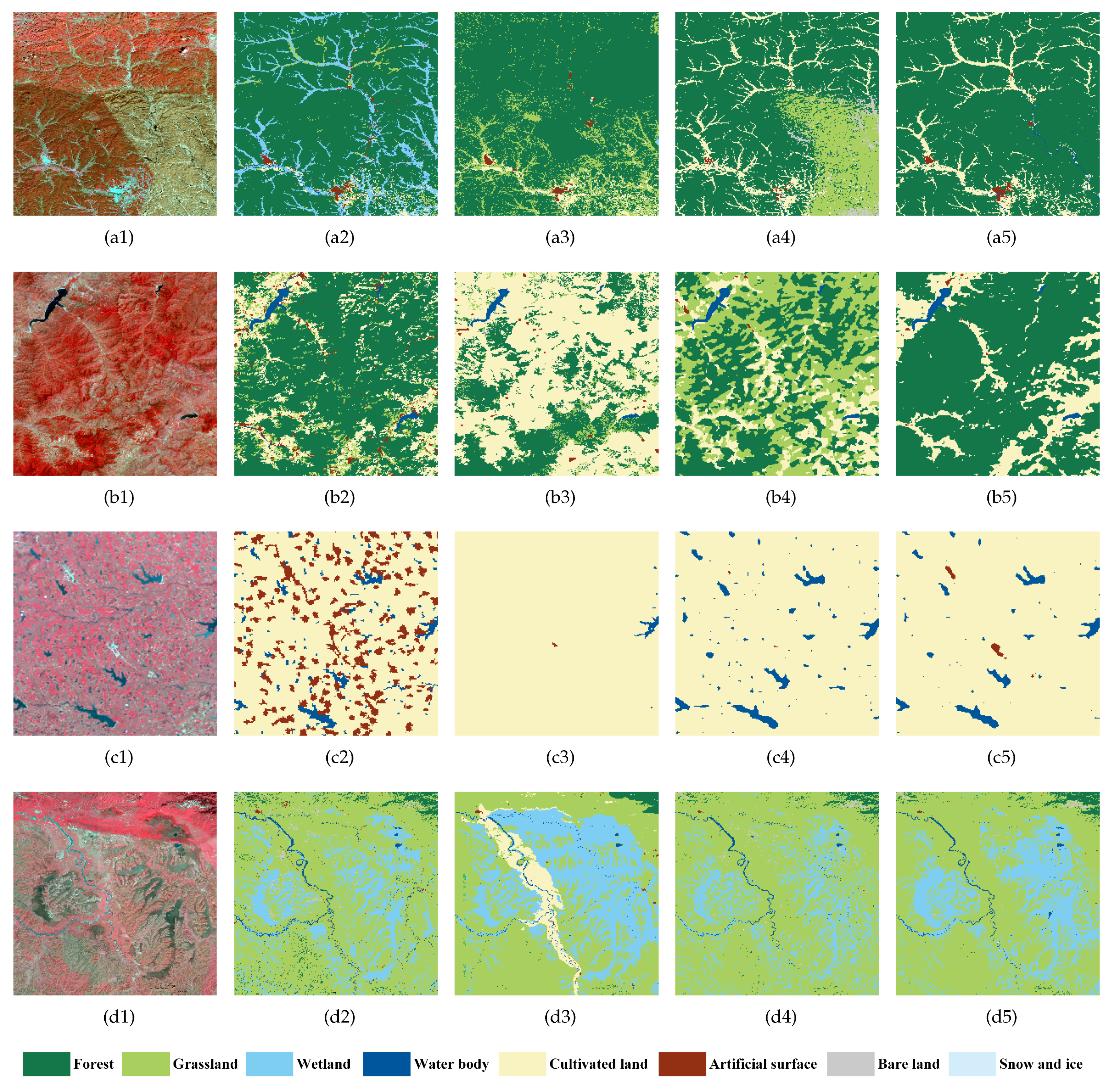
5.2. Qualitative Results for Typical Regions

To test the efficiency of the proposed MTNet, we compared with the most widely used methods in large-scale remote sensing image classification (to make a fair comparison, all the network employed in this study took PSPNet as a backbone), including: (1) traditional random forest (RF) classifier, which was demonstrated to be the most effective method [63]; (2) PSPNet-RL, which employed a robust loss proposed in [54] to alleviate the impact of noisy labels; (3) PSPNet trained by a training set collected outside the current data (we called it PSPNet-TF in this study); (4) the traditional PSPNet. The above-mentioned algorithms and the proposed MTNet were performed on the training set introduced in Section 3.3.2.

Detailed results for the performance of the model for Liaoning, Hubei and Qinghai are shown in Figure 6, Figure 7 and Figure 8. RF uses pixel-wise training samples to train the classifier. The lack of context relationship makes it sensitive to noise. Accordingly, the corresponding classification results were not satisfactory. In fact, the class noise contained in the training samples also had a great impact on RF. As demonstrated in the last subsection, the training samples were derived from existing land cover maps and contained some class noise. Since the RF classifier does not need a pixel-wise-labeled image patch, the center pixel of a training sample was selected as a training point to construct a training set for the RF classifier. Actually, we tried to select 1–30 pixels from each image as training samples and even used all the training samples, both randomly or following certain rules. However, there was no significant difference on the training or testing precision due to the capacity of the RF classifier. Considering the trade-off between the precision and the training efficiency, we randomly selected five pixels from each image and constructed a training set with 67,301 sample points by removing pixels, which were labeled as others.

It is clear that the PSPNet was sensitive to the training samples that were used. Its recognition ability was significantly reduced when the original Landsat image contained features that were obviously inconsistent with the training samples. Benefiting from the robust loss in PSPNet-RL, the noisy resistant ability was slightly improved. This also decreased the recognition ability of PSPNet-RL on objects that contained complex features, such as Figure 6(b4,d4), Figure 7(b4,c4) and Figure 8(a4), etc. PSPNet obtained better classification results than PSPNet-TF, which was trained with samples outside the current time periods. Overall, the models trained using the 2010 training set had a stronger generalization ability than the models trained using the 2005 training set. This was because the 2010 training set was of better quality. Using the consistent information provided by the 2010 training set, PSPNet was able to learn the image features more efficiently. The MTNet was fine-tuned using the current training set. The parameters of the MTNet were determined by time series training sets. This means that the MTNet was able to learn more general features from the current training set while maintaining the stable feature-learning ability acquired from the time series training set. In this way, the MTNet can overcome the drawback of having imbalanced training samples and learn essential features from noisy labels. As shown in the results in Figure 6, Figure 7 and Figure 8, the classification for MTNet were the best among all the models and sometimes outperformed even the reference, visually.

5.3. Quantitative Results for Typical Region

Using the training set introduced in Section 3.3.2, the precision and F1_score for the study areas are listed in

Table 4. Precision and F1_score for the study areas (Liaoning, Hubei and Qinghai provinces).

	Time Period	RF		PSPNet-RL		PSPNet		PSPNet-TF		MTNet
(%)		Precision	F1_Score	Precision	F1_Score	Precision	F1_Score	Precision	F1_Score
Liaoning	2005	47.76	49.79	71.80	71.39	72.97	72.44	71.69	71.80	73.58	73.21
	2010	54.04	54.04	84.52	83.31	83.39	82.94	81.14	80.98	83.94	83.04
Hubei	2005	51.16	58.02	80.91	79.47	81.13	79.78	79.10	77.70	81.32	80.04
	2010	52.40	59.06	77.70	76.60	76.96	75.82	77.50	76.26	80.68	80.09
Qinghai	2005	51.40	55.81	73.97	74.16	71.57	72.16	71.89	72.03	74.49	74.62
	2010	52.79	56.92	71.86	72.24	65.77	65.57	68.03	67.77	75.48	75.36

. It can be seen that:

(1)

Among all the methods: RF obtained the lowest accuracy. Influenced by the independence in training samples, RF cannot effectively learn the relationship between pixels and thus is sensitive to noise. Accordingly, both the precision and the F1_score were significantly lower than DL-based methods.

(2)

Generally, PSPNet-RL obtained better accuracies than the PSPNet, due to the introduced robust loss function. This means the robust loss proposed in [54] does have the ability of improving the robustness to noisy labels. However, as shown in Figure 6, Figure 7 and Figure 8, this improvement in the classification accuracy is at the cost of decreasing the recognition ability of complex features. Unfortunately, for most applications, object recognition ability is much more important than accuracy.

(3)

For Liaoning province at different time periods, the difference in the precision and F1_score for the years 2005 and 2010 were all notable: this was caused by the quality of the original images. The Landsat imagery of the west of Liaoning that was acquired in 2005 included some images from outside the growing season; this had a great impact on the ability to recognize vegetation types. Therefore, both the precision and the F1_score for 2005 were obviously lower than those for 2010.

(4)

For Hubei and Qinghai provinces at different time periods, all the accuracies of Liaoning in 2010 were higher than those in 2005, since the training samples contained images obtained in non-growing seasons. Accordingly, models trained by the 2010 training set had higher accuracies than those trained by the 2005 training set. This phenomenon was not found in Hubei and Qinghai. This demonstrates that models trained using high-quality training samples are more general than models trained using poorer-quality training samples.

(5)

For the same study area in the same year, PSPNet-RL outperformed PSPNet, and PSPNet outperformed PSPNet-TF, while all the classification accuracies of the MTNet were higher than the others. The MTNet performed well even when the training samples were not balanced and noisy labels were included. The use of interactive training samples from time-series data significantly improved the performance of the networks. This demonstrates the efficiency of the mutual training strategy used in the MTNet.

(6)

For different study areas, the overall accuracies were affected by the quality of the original images and labels, and so they varied with the study areas. This was a result of the different proportions of each class that were present in the training samples. For example, the main classes made up a large proportion of the training samples for Liaoning and Hubei. As a result, the overall accuracies for these areas were higher than for Qinghai, for which the samples corresponding to the main classes were of poor quality or contained noisy labels.

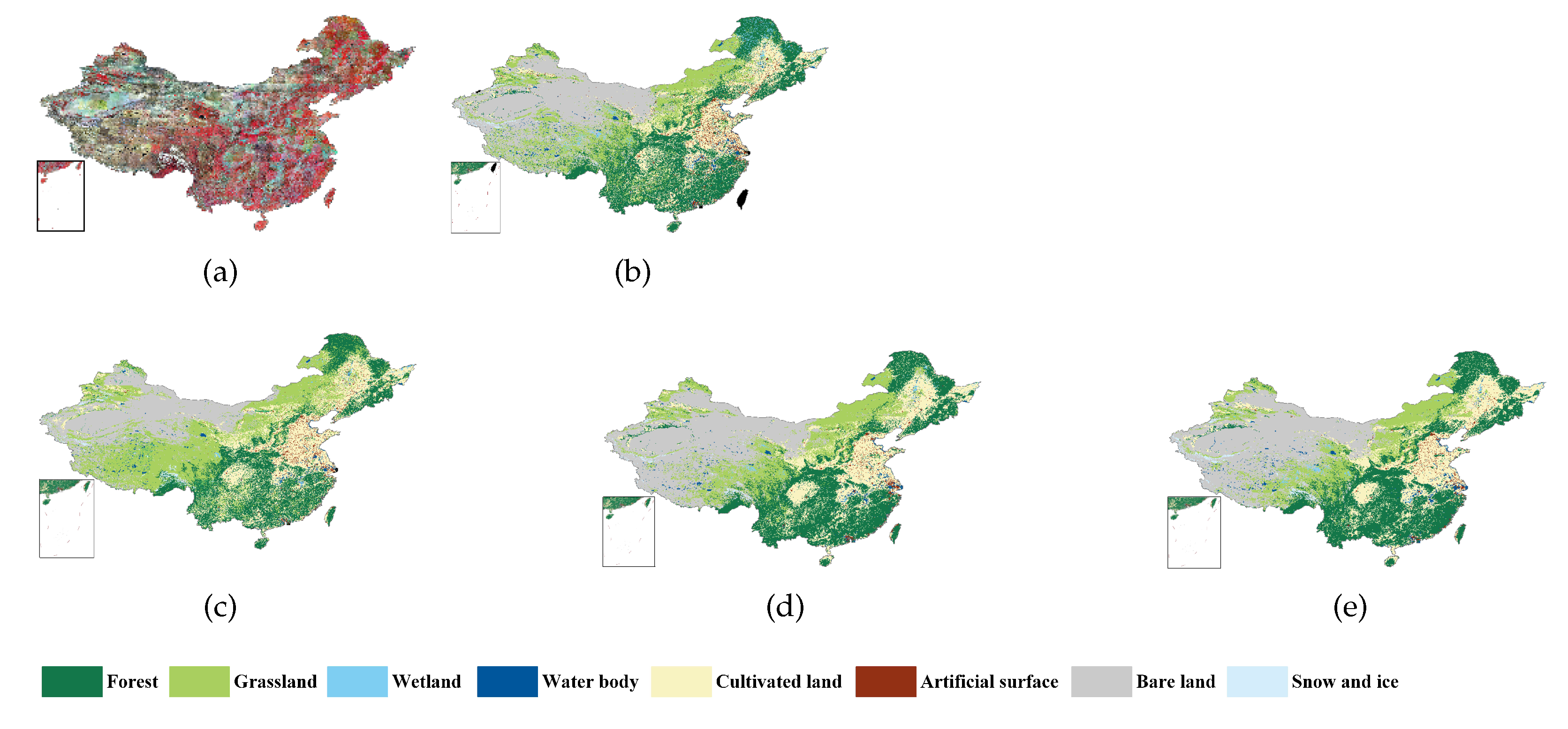
6. Extension to Land Cover Maps of China

Most of the existing land cover maps were produced by point-based classifiers, such as MLC, DT, RF and SVM. Point-based training sets are easy to access, and the quality is highly guaranteed. This greatly shortens the training time of the model and ensures the learning efficiency of the classifiers. However, restricted by the limited information contained in small training sets and the essential driver of the classifiers, traditional point-based classifiers are sensitive to the variation of features representing the same class. This leads to poor performance on large-scale study areas, which is the reason why the production of large-scale land cover products need complex pre- and post-processing and a large amount of human interaction. This means using the RF classifier in the last section cannot obtain comparable accuracy with existing land cover maps. With the rapid development of remote sensing techniques, this kind of classifier cannot meet the rapid development of application demand. DL-based methods use a large amount of parameters to learn from massive information contained in pixel-wise-labeled training samples, and even it suffers from imbalanced and noisy labels. This increases the suitability of the DL-based method on large-scale study areas. Nevertheless, the learning ability of the DL-based method is highly dependent on the quality of the training set. Benefiting from the transferability of the DL-based method, the proposed MTNet mutually transfers pretrained models to other time periods and jointly learns general information in time series training samples. This obviously increases its robustness on imbalanced and noisy labels. To further test the proposed MTNet and also to provide a solution for large-scale land cover mapping, the MTNet was used to produce a new national land cover map of China in 2010. The produced land cover map was qualitatively compared with existing products as shown in Figure 9.

The original Landsat images for 2010 were only stitched without any pre-processing. Therefore, the stitching lines were obvious as shown in Figure 9a. Actually, the original Landsat images wereexactly the ones used for producing all the land cover maps except Figure 9b. The Land Cover Map of People’s Republic of China (LCMPRC) is the most accurate land cover product we know. However, there are some obvious errors in northeast China, where the cultivated land was classified as wetland as shown in Figure 9b. The GlobalLandCover 30 (GLC30) contained 10 first-level classes and was merged to the proposed 8 first-level classes listed in Table 1. In Figure 9c, most of Qinghai–Tibet was classified as grassland where they should be bare land according to Figure 9a. The classification results of PSPNet and MTNet were similar, from a national perspective.

To further explore the difference among all the land cover maps, detailed classification results are shown in Figure 10. Figure 10(a1) is an area stitched from multi-images, where the lower-right part comes from non-growing seasons. PSPNet classifies this area as grassland, while the proposed MTNet can correctly recognize this area as forest. Figure 10(a2) shows the details of the misclassification of cultivated land to wetland in the northeast China of LCMPRC. GLC30 cannot obtain a satisfactory result in this area as shown in Figure 10(a3). Figure 10(b1) is mostly covered by forest (darker red part) and cultivated land (lighter red part). LCMPRC can distinguish different classes, but the result is fragmented. GLC30 classifies some forest as cultivated land, while PSPNet classifies some forest as grassland. The classification results of MTNet are promising compared with other land cover maps. Figure 10(c1) is an atypical landform in China, and it can only be found in the middle east area. LCMPRC misclassified some of the cultivated land as an artificial surface, and even typical features of artificial surface exist in this area (as shown in Figure 10(a2)). GLC30 cannot recognize the water body with such salient features and classifies them as cultivated land. PSPNet is able to recognize the water bodies but misses the features of artificial surfaces. Benefiting from time series training samples, MTNet is more robust to changes of features in the same class and obtains satisfactory classification results (as shown in Figure 10(c5)). Influenced by the nature distribution of different classes all over China, wetland occupies the least proportion. Accordingly, the training samples for wetland is less efficient compared with other classes. This has a great impact on both traditional point-based classifiers and DL-based methods (as shown in Figure 10(d2,d4)). Besides, the similarity between features of different classes also has a great impact on the recognition ability of traditional classifiers, as shown in Figure 10(d3). The MTNet jointly learns from time series training samples and is able to learn more information and obtain better classification results.

From a quantitative evaluation point of view, traditional point-based evaluation may over-estimate the accuracies since sample points have a higher probability to lie in the middle of an object, while misclassification is more likely to appear near the boundary. To roughly estimate the classification results of PSPNet and MTNet, we randomly selected 15 images with 10,240 × 10,240 pixels as an estimation area and then calculated the precision and F1_score by considering the GLC30 and LCMPRC as the ground truth, respectively. The corresponding results are listed in

Table 5. Jointly Comparison Results.

Base	GLC30		LCMPRC		PSPNet		MTNet
	Precision	F1_Score	Precision	F1_Score	Precision	F1_Score	Precision	F1_Score
GLC30	-		74.21	62.63	77.05	63.74	77.55	64.03
LCMPRC	74.50	59.77	-		82.51	64.38	82.61	64.41

. It was clear that: (1) the evaluation results based on LCMPRC were much higher than those based on GLC30. That was caused by the accuracy of the base, which was considered as the ground truth. The overall accuracy of GLC30 was about 80%, while it was between 86% and 94% for LCMPRC. This means the evaluation results based on LCMPRC were more accurate than those based on GLC30. (2) Under this evaluation criteria, DL-based methods (PSPNet and MTNet) outperformed traditional ones (GLC30, which is a combination of MLC, DT, SVM and human labors, and LCMPRC, which is produced by many cooperative institutes). Benefiting from the large amount of parameters, DL-based methods can learn more from the training samples and outperform traditional classifiers. (3) MTNet outperformed PSPNet to some extent. As shown in the detailed results of GLC30 and LCMPRC in Figure 10, these two products may be superior in some classes in some areas, but they also contain obvious misclassified areas. That may have an impact on the evaluation results. Actually, jointly learning from time series training samples allows MTNet to learn more essential information than PSPNet. Overall, MTNet provides a new idea for large-scale land cover mapping, and its classification result is promising compared with existing ones.

7. Conclusions

A mutual transfer network (MTNet) for large-scale time-series land-cover mapping was proposed. After comparing the performances of PSPNet, PSPNet-RL, PSPNet-TF and MTNet, we proposed an idea for large-scale land cover mapping. It was demonstrated by experiment that, as also stated in [20], the quality of the training samples had a significant impact on the classification results. Based on the transferability of CNN, the proposed MTNet can take advantage of the time-series of training samples and obtain better classification results than a traditional training strategy based on an imbalanced training set with noisy labels. This study provides a solution for practical large-scale land cover mapping, but it did not take the consistency between time series land cover mapping into consideration. Large-scale land cover maps produced by MTNet can be post-processed according to [64,65].

The DL-based method provides a new opportunity for producing large-scale land cover maps. In future work, we will focus on introducing training samples with different imaging times to improve the recognition ability of the DL-based method, especially for vegetation. We will also try to introduce domain adaption and change detection methods into MTNet to improve its generality for large-scale land cover mapping.

References

1. Kwan, C.; Gribben, D.; Ayhan, B.; Li, J.; Bernabe, S.; Plaza, A. An Accurate Vegetation and Non-Vegetation Differentiation Approach Based on Land Cover Classification. Remote Sens. 2020, 12, 3880. [Google Scholar] [CrossRef]
2. Hong, D.; Hu, J.; Yao, J.; Chanussot, J.; Zhu, X.X. Multimodal remote sensing benchmark datasets for land cover classification with a shared and specific feature learning model. ISPRS J. Photogramm. Remote Sens. 2021, 178, 68–80. [Google Scholar] [CrossRef] [PubMed]
3. Vogelmann, J.E.; Howard, S.M.; Yang, L.; Larson, C.R.; Wylie, B.K.; Van Driel, N. Completion of the 1990s National Land Cover Data Set for the conterminous United States from Landsat Thematic Mapper data and ancillary data sources. Photogramm. Eng. Remote Sens. 2001, 67, 650–662. [Google Scholar]
4. Hong, D.; Yokoya, N.; Chanussot, J.; Zhu, X.X. An Augmented Linear Mixing Model to Address Spectral Variability for Hyperspectral Unmixing. IEEE Trans. Image Process. 2019, 28, 1923–1938. [Google Scholar] [CrossRef] [Green Version]
5. Ma, L.; Li, M.; Ma, X.; Cheng, L.; Du, P.; Liu, Y. A review of supervised object-based land-cover image classification. ISPRS J. Photogramm. Remote Sens. 2017, 130, 277–293. [Google Scholar] [CrossRef]
6. Maselli, F.; Conese, C.; De Filippis, T.; Romani, M. Integration of ancillary data into a maximum-likelihood classifier with nonparametric priors. ISPRS J. Photogramm. Remote Sens. 1995, 50, 2–11. [Google Scholar] [CrossRef]
7. Bruzzone, L.; Prieto, D.F. Unsupervised retraining of a maximum likelihood classifier for the analysis of multitemporal remote sensing images. IEEE Trans. Geosci. Remote Sens. 2001, 39, 456–460. [Google Scholar] [CrossRef] [Green Version]
8. Quinlan, J.R. Induction of Decision Trees. Mach. Learn. 1986, 1, 81–106. [Google Scholar] [CrossRef] [Green Version]
9. Quinlan, J.R. C4.5: Programs for Machine Learning; Mach Learn; Morgan Kaufmann Publishers: Burlington, MA, USA, 1994; Volume 16, pp. 235–240. [Google Scholar]
10. Colditz, R.R. An Evaluation of Different Training Sample Allocation Schemes for Discrete and Continuous Land Cover Classification Using Decision Tree-Based Algorithms. Remote Sens. 2015, 7, 9655–9681. [Google Scholar] [CrossRef] [Green Version]
11. Breiman, L. Random forest. Mach. Learn. 2001, 45, 5–32. [Google Scholar] [CrossRef] [Green Version]
12. Belgiu, M.; Drăguţ, L. Random forest in remote sensing: A review of applications and future directions. ISPRS J. Photogramm. Remote Sens. 2016, 114, 24–31. [Google Scholar] [CrossRef]
13. Sain, S.R. The Nature of Statistical Learning Theory. Technometrics 1996, 38, 409-409. [Google Scholar] [CrossRef]
14. Mountrakis, G.; Im, J.; Ogole, C. Support vector machines in remote sensing: A review. ISPRS J. Photogramm. Remote Sens. 2011, 66, 247–259. [Google Scholar] [CrossRef]
15. Hong, D.; Gao, L.; Yao, J.; Zhang, B.; Plaza, A.; Chanussot, J. Graph Convolutional Networks for Hyperspectral Image Classification. IEEE Trans. Geosci. Remote Sens. 2020, 59, 5966–5978. [Google Scholar] [CrossRef]
16. Hong, D.; Gao, L.; Yokoya, N.; Yao, J.; Chanussot, J.; Du, Q.; Zhang, B. More Diverse Means Better: Multimodal Deep Learning Meets Remote-Sensing Imagery Classification. IEEE Trans. Geosci. Remote Sens. 2021, 59, 4340–4354. [Google Scholar] [CrossRef]
17. Long, J.; Shelhamer, E.; Darrell, T. Fully Convolutional Networks for Semantic Segmentation. IEEE Trans. Pattern Anal. Mach. Intell. 2017, 39, 640–651. [Google Scholar]
18. Ronneberger, O.; Fischer, P.; Brox, T. U-Net: Convolutional Networks for Biomedical Image Segmentation. In Medical Image Computing and Computer-Assisted Intervention–MICCAI 2015; Navab, N., Hornegger, J., Wells, W.M., Frangi, A.F., Eds.; Springer International Publishing: Cham, Munich, Germany, 2015; pp. 234–241. [Google Scholar]
19. Zhao, H.; Shi, J.; Qi, X.; Wang, X.; Jia, J. Pyramid Scene Parsing Network. In Proceedings of the 2017 IEEE Conference on Computer Vision and Pattern Recognition (CVPR), Honolulu, HI, USA, 21–26 July 2017; pp. 6230–6239. [Google Scholar]
20. Gong, P.; Yu, L.; Li, C.; Wang, J.; Liang, L.; Li, X.; Ji, L.; Bai, Y.; Cheng, Y.; Zhu, Z. A new research paradigm for global land cover mapping. Ann. GIS 2016, 22, 87–102. [Google Scholar] [CrossRef] [Green Version]
21. Li, C.; Wang, J.; Wang, L.; Hu, L.; Gong, P. Comparison of Classification Algorithms and Training Sample Sizes in Urban Land Classification with Landsat Thematic Mapper Imagery. Remote Sens. 2014, 6, 964–983. [Google Scholar] [CrossRef] [Green Version]
22. Radoux, J.; Lamarche, C.; Van Bogaert, E.; Bontemps, S.; Brockmann, C.; Defourny, P. Automated Training Sample Extraction for Global Land Cover Mapping. Remote Sens. 2014, 6, 3965–3987. [Google Scholar] [CrossRef] [Green Version]
23. Zhang, X.; Liu, L.; Chen, X.; Xie, S.; Gao, Y. Fine Land-Cover Mapping in China Using Landsat Datacube and an Operational SPECLib-Based Approach. Remote Sens. 2019, 11, 1056. [Google Scholar] [CrossRef] [Green Version]
24. Koziarski, M.; Woźniak, M.; Krawczyk, B. Combined Cleaning and Resampling algorithm for multi-class imbalanced data with label noise. Knowl.-Based Syst. 2020, 204, 106223. [Google Scholar] [CrossRef]
25. Patrini, G.; Rozza, A.; Menon, A.K.; Nock, R.; Qu, L. Making Deep Neural Networks Robust to Label Noise: A Loss Correction Approach. In Proceedings of the 2017 IEEE Conference on Computer Vision and Pattern Recognition (CVPR), Honolulu, HI, USA, 21–26 July 2017; pp. 2233–2241. [Google Scholar]
26. Tanaka, D.; Ikami, D.; Yamasaki, T.; Aizawa, K. Joint Optimization Framework for Learning with Noisy Labels. In Proceedings of the 2018 IEEE/CVF Conference on Computer Vision and Pattern Recognition, Salt Lake City, UT, USA, 18–22 June 2018; pp. 5552–5560. [Google Scholar]
27. Hong, D.; Yokoya, N.; Chanussot, J.; Xu, J.; Zhu, X.X. Joint and Progressive Subspace Analysis (JPSA) With Spatial–Spectral Manifold Alignment for Semisupervised Hyperspectral Dimensionality Reduction. IEEE Trans. Cybern. 2021, 51, 3602–3615. [Google Scholar] [CrossRef]
28. Liu, T.; Tao, D. Classification with Noisy Labels by Importance Reweighting. IEEE Trans. Pattern Anal. Mach. Intell. 2016, 38, 447–461. [Google Scholar] [CrossRef] [Green Version]
29. Ghosh, A.; KUmar, H.; Sastry, P. Robust loss functions under labelnoise for deep neural networks. In Proceedings of the AAAI Conference on Artificial and Intelligence, San Francisco, CA, USA, 4–9 February 2017; pp. 1919–1925. [Google Scholar]
30. Rezaee, M.; Mahdianpari, M.; Zhang, Y.; Salehi, B. Deep Convolutional Neural Network for Complex Wetland Classification Using Optical Remote Sensing Imagery. IEEE J. Sel. Top. Appl. Earth Obs. Remote Sens. 2018, 11, 3030–3039. [Google Scholar] [CrossRef]
31. Krizhevsky, A.; Sutskever, I.; Hinton, G. ImageNet classification with deep convolutional neural networks. Commun. ACM 2012, 25, 84–90. [Google Scholar] [CrossRef]
32. Huang, B.; Zhao, B.; Song, Y. Urban land-use mapping using a deep convolutional neural network with high spatial resolution multispectral remote sensing imagery. Remote Sens. Environ. 2018, 214, 73–86. [Google Scholar] [CrossRef]
33. Marmanis, D.; Datcu, M.; Esch, T.; Stilla, U. Deep Learning Earth Observation Classification Using ImageNet Pretrained Networks. IEEE Geosci. Remote Sens. Lett. 2016, 13, 105–109. [Google Scholar] [CrossRef] [Green Version]
34. Scott, G.J.; England, M.R.; Starms, W.A.; Marcum, R.A.; Davis, C.H. Training Deep Convolutional Neural Networks for Land–Cover Classification of High-Resolution Imagery. IEEE Geosci. Remote Sens. Lett. 2017, 14, 549–553. [Google Scholar] [CrossRef]
35. Chen, Y.; Ming, D.; Lv, X. Superpixel based land cover classification of VHR satellite image combining multi-scale CNN and scale parameter estimation. Earth Sci. Inform. 2019, 12, 341–363. [Google Scholar] [CrossRef]
36. Liu, S.; Qi, Z.; Li, X.; Yeh, A.G.O. Integration of Convolutional Neural Networks and Object-Based Post-Classification Refinement for Land Use and Land Cover Mapping with Optical and SAR Data. Remote Sens. 2019, 11, 690. [Google Scholar] [CrossRef] [Green Version]
37. Zhang, S.; Li, C.; Qiu, S.; Gao, C.; Zhang, F.; Du, Z.; Liu, R. EMMCNN: An ETPS-Based Multi-Scale and Multi-Feature Method Using CNN for High Spatial Resolution Image Land-Cover Classification. Remote Sens. 2020, 12, 66. [Google Scholar] [CrossRef] [Green Version]
38. Hu, Y.; Zhang, Q.; Zhang, Y.; Yan, H. A Deep Convolution Neural Network Method for Land Cover Mapping: A Case Study of Qinhuangdao, China. Remote Sens. 2018, 10, 2053. [Google Scholar] [CrossRef] [Green Version]
39. Marcos, D.; Volpi, M.; Kellenberger, B.; Tuia, D. Land cover mapping at very high resolution with rotation equivariant CNNs: Towards small yet accurate models. ISPRS J. Photogramm. Remote Sens. 2018, 145, 96–107. [Google Scholar] [CrossRef] [Green Version]
40. Li, W.; Dong, R.; Fu, H.; Wang, J.; Yu, L.; Gong, P. Integrating Google Earth imagery with Landsat data to improve 30-m resolution land cover mapping. Remote Sens. Environ. 2020, 237, 111563. [Google Scholar] [CrossRef]
41. Hong, D.; Yokoya, N.; Xia, G.S.; Chanussot, J.; Zhu, X.X. X-ModalNet: A semi-supervised deep cross-modal network for classification of remote sensing data. ISPRS J. Photogramm. Remote. Sens. 2020, 167, 12–23. [Google Scholar] [CrossRef]
42. Nijhawan, R.; Joshi, D.; Narang, N.; Mittal, A.; Mittal, A.A. A Futuristic Deep Learning Framework Approach for Land Use-Land Cover Classification Using Remote Sensing Imagery. In Advanced Computing and Communication Technologies; Mandal, J.K., Bhattacharyya, D., Auluck, N., Eds.; Springer: Singapore, 2019; pp. 87–96. [Google Scholar]
43. Zhang, C.; Pan, X.; Li, H.; Gardiner, A.; Sargent, I.; Hare, J.; Atkinson, P.M. A hybrid MLP-CNN classifier for very fine resolution remotely sensed image classification. ISPRS J. Photogramm. Remote Sens. 2018, 140, 133–144. [Google Scholar] [CrossRef] [Green Version]
44. Zhang, C.; Sargent, I.; Pan, X.; Li, H.; Gardiner, A.; Hare, J.; Atkinson, P.M. Joint Deep Learning for land cover and land use classification. Remote Sens. Environ. 2019, 221, 173–187. [Google Scholar] [CrossRef] [Green Version]
45. Jiang, J.; Ma, J.; Wang, Z.; Chen, C.; Liu, X. Hyperspectral Image Classification in the Presence of Noisy Labels. IEEE Trans. Geosci. Remote Sens. 2019, 57, 851–865. [Google Scholar] [CrossRef] [Green Version]
46. Santos, L.A.; Ferreira, K.R.; Camara, G.; Picoli, M.C.; Simoes, R.E. Quality control and class noise reduction of satellite image time series. ISPRS J. Photogramm. Remote Sens. 2021, 177, 75–88. [Google Scholar] [CrossRef]
47. Algan, G.; Ulusoy, I. Image classification with deep learning in the presence of noisy labels: A survey. Knowl.-Based Syst. 2021, 215, 106771. [Google Scholar] [CrossRef]
48. Zhang, J.; Dai, Y.; Zhang, T.; Harandi, M.; Barnes, N.; Hartley, R. Learning Saliency From Single Noisy Labelling: A Robust Model Fitting Perspective. IEEE Trans. Pattern Anal. Mach. Intell. 2021, 43, 2866–2873. [Google Scholar]
49. Ji, D.; Oh, D.; Hyun, Y.; Kwon, O.M.; Park, M.J. How to handle noisy labels for robust learning from uncertainty. Neural Netw. 2021, 143, 209–217. [Google Scholar] [CrossRef]
50. Deng, L.; Yang, B.; Kang, Z.; Yang, S.; Wu, S. A noisy label and negative sample robust loss function for DNN-based distant supervised relation extraction. Neural Netw. 2021, 139, 358–370. [Google Scholar] [CrossRef]
51. Han, B.; Tsang, I.W.; Chen, L.; Zhou, J.T.; Yu, C.P. Beyond Majority Voting: A Coarse-to-Fine Label Filtration for Heavily Noisy Labels. IEEE Trans. Neural Netw. Learn. Syst. 2019, 30, 3774–3787. [Google Scholar] [CrossRef]
52. Zhang, X.Y.; Liu, C.L.; Suen, C.Y. Towards Robust Pattern Recognition: A Review. Proc. IEEE 2020, 108, 894–922. [Google Scholar] [CrossRef]
53. Zhang, Q.; Lee, F.; Wang, Y.; Miao, R.; Chen, L.; Chen, Q. An improved noise loss correction algorithm for learning from noisy labels. J. Vis. Commun. Image Represent. 2020, 72, 102930. [Google Scholar] [CrossRef]
54. Xu, Y.; Li, Z.; Li, W.; Du, Q.; Liu, C.; Fang, Z.; Zhai, L. Dual-Channel Residual Network for Hyperspectral Image Classification With Noisy Labels. IEEE Trans. Geosci. Remote Sens. 2021. [Google Scholar] [CrossRef]
55. Zhang, Q.; Lee, F.; Wang, Y.; Ding, D.; Yao, W.; Chen, L.; Chen, Q. An joint end-to-end framework for learning with noisy labels. Appl. Soft Comput. 2021, 108, 107426. [Google Scholar] [CrossRef]
56. Dube, T.; Mutanga, O.; Ismail, R. Quantifying aboveground biomass in African environments: A review of the trade-offs between sensor estimation accuracy and costs. Trop. Ecol. 2016, 57, 393–405. [Google Scholar]
57. Massetti, A.; Gil, A. Mapping and assessing land cover/land use and aboveground carbon stocks rapid changes in small oceanic islands’ terrestrial ecosystems: A case study of Madeira Island, Portugal (2009–2011). Remote Sens. Environ. 2020, 239, 111625. [Google Scholar] [CrossRef]
58. Jiang, M.; Yong, B.; Tian, X.; Malhotra, R.; Hu, R.; Li, Z.; Yu, Z.; Zhang, X. The potential of more accurate InSAR covariance matrix estimation for land cover mapping. ISPRS J. Photogramm. Remote Sens. 2017, 126, 120–128. [Google Scholar] [CrossRef]
59. Sánchez-Espinosa, A.; Schröder, C. Land use and land cover mapping in wetlands one step closer to the ground: Sentinel-2 versus landsat 8. J. Environ. Manag. 2019, 247, 484–498. [Google Scholar] [CrossRef]
60. Gong, P.; Wang, J.; Yu, L.; Zhao, Y.; Zhao, Y.; Liang, L.; Niu, Z.; Huang, X.; Fu, H.; Liu, S.; et al. Finer resolution observation and monitoring of global land cover: First mapping results with Landsat TM and ETM+ data. Int. J. Remote Sens. 2013, 34, 2607–2654. [Google Scholar] [CrossRef] [Green Version]
61. Huang, H.; Wang, J.; Liu, C.; Liang, L.; Li, C.; Gong, P. The migration of training samples towards dynamic global land cover mapping. ISPRS J. Photogramm. Remote Sens. 2020, 161, 27–36. [Google Scholar] [CrossRef]
62. Gong, P.; Liu, H.; Zhang, M.; Li, C.; Wang, J.; Huang, H.; Clinton, N.; Ji, L.; Li, W.; Bai, Y.; et al. Stable classification with limited sample: Transferring a 30-m resolution sample set collected in 2015 to mapping 10-m resolution global land cover in 2017. Sci. Bull. 2019, 64, 370–373. [Google Scholar] [CrossRef] [Green Version]
63. Chen, J.; Chen, J.; Liao, A.; Cao, X.; Chen, L.; Chen, X.; He, C.; Han, G.; Peng, S.; Lu, M.; et al. Global land cover mapping at 30m resolution: A POK-based operational approach. ISPRS J. Photogramm. Remote Sens. 2015, 103, 7–27. [Google Scholar] [CrossRef] [Green Version]
64. Liu, S.; Su, H.; Cao, G.; Wang, S.; Guan, Q. Learning from data: A post classification method for annual land cover analysis in urban areas. ISPRS J. Photogramm. Remote Sens. 2019, 154, 202–215. [Google Scholar] [CrossRef]
65. Maus, V.; Câmara, G.; Cartaxo, R.; Sanchez, A.; Ramos, F.M.; de Queiroz, G.R. A Time-Weighted Dynamic Time Warping Method for Land-Use and Land-Cover Mapping. IEEE J. Sel. Top. Appl. Earth Obs. Remote Sens. 2016, 9, 3729–3739. [Google Scholar] [CrossRef]
Figure 1. Location of the Jing-Jin-Ji region within China.
Remotesensing 13 04194 g001
Figure 2. Locations of the study areas in China.
Remotesensing 13 04194 g002
Figure 3. Original Landsat 5 Level 1T images of China (pseudo-color combined of NIR, red and green bands). (a) 2005; (b) 2010.
Remotesensing 13 04194 g003
Figure 4. Proportions of different classes for China and on the training set.
Remotesensing 13 04194 g004
Figure 5. Flowchart of MTNet. Training set of Time 1 was used to train the PSPNet. Then, the trained network was finetuned by the training set of Time 2 to make the network suitable for land cover mapping of images in Time 2.
Remotesensing 13 04194 g005
Figure 6. Detailed classification results for Liaoning, where (a1d1) are the original Landsat images, (a2d2) are the reference, (a3d3) are classification results for RF classifier, (a4d4) are classification results of PSPNet-RL, (a5d5) are classification results of PSPNet, (a6d6) are classification results of PSPNet-TF and (a7d7) are classification results of MTNet. The results shown in (a1b7) are for the year 2005; the results shown in (c1d7) are for 2010.
Remotesensing 13 04194 g006
Figure 7. Detailed classification results for Hubei, where (a1d1) are the original Landsat images, (a2d2) are the reference, (a3d3) are classification results for RF classifier, (a4d4) are classification results of PSPNet-RL, (a5d5) are classification results of PSPNet, (a6d6) are classification results of PSPNet-TF, and (a7d7) are classification results of MTNet. The results shown in (a1b7) are for the year 2005; the results shown in (c1d7) are for 2010.
Remotesensing 13 04194 g007
Figure 8. Detailed classification results for Qinghai, where (a1d1) are the original Landsat images, (a2d2) are the reference, (a3d3) are classification results for RF classifier, (a4d4) are classification results of PSPNet-RL, (a5d5) are classification results of PSPNet, (a6d6) are classification results of PSPNet-TF and (a7d7) are classification results of MTNet. The results shown in (a1b7) are for the year 2005; the results shown in (c1d7) are for 2010.
Remotesensing 13 04194 g008
Figure 9. Original Landsat images for 2010 and corresponding land cover maps, where (a) is composed of 1056 Landsat 5 image with obvious stitching lines (https://earthexplorer.usgs.gov, accessed on 10 December 2017); (b) is the Land Cover Map of People’s Republic of China with an overall accuracy between 86% to 94% (http://www.geodata.cn, accessed on 10 December 2017); (c) is the GlobalLandCover 30 (GLC30) with an overall accuracy about 80% [63]; (d) is the land cover map produced by PSPNet and (e) is the land cover map produced by the proposed MTNet.
Remotesensing 13 04194 g009
Figure 10. Detailed classification results for the original Landsat images and corresponding land cover maps, where (a1d1) are original Landsat images, which were used for the producing of GLC30 and the results of PSPNet and MTNet; (a2d2) are classification results from the Land Cover Map of People’s Republic of China; (a3d3) are classification results from the GLC30; (a4d4) are classification results of PSPNet and (a5d5) are classification results of MTNet.
Remotesensing 13 04194 g010