Article

Detecting the Complex Relationships and Driving Mechanisms of Key Ecosystem Services in the Central Urban Area Chongqing Municipality, China

1
Faculty of Architecture and Urban Planning, Chongqing University, Chongqing 400030, China
2
Research Center for Ecological Restoration and Control of Water Level Fluctuating Zone in the Three Gorges Reservoir Area, Chongqing University, Chongqing 400030, China
3
Ministry of Education Key Laboratory of the Three Gorges Reservoir Region’s Eco-Environment, Chongqing University, Chongqing 400044, China
4
School of Civil Engineering, Chongqing Jiaotong University, Chongqing 400074, China
*
Author to whom correspondence should be addressed.
Remote Sens. 2021, 13(21), 4248; https://0-doi-org.brum.beds.ac.uk/10.3390/rs13214248
Submission received: 1 September 2021 / Revised: 16 October 2021 / Accepted: 18 October 2021 / Published: 22 October 2021

Abstract

:
Ecosystem services (ESs) are highly vulnerable to human activities. Understanding the relationships among multiple ESs and driving mechanisms are crucial for multi-objective management in complex social-ecological systems. The goals of this study are to quantitatively evaluate and identify ESs hotspots, explore the relationships among ESs and elucidate the driving mechanisms. Taking central urban area Chongqing municipality as the study area, biodiversity (BI), carbon fixation (CF), soil conservation (SC) and water conservation (WC) were evaluated based on the InVEST model and ESs hotspots were identified. The complex interactions among multiple ESs were determined by utilizing multiple methods: spearman correlation analysis, bivariate local spatial autocorrelation and K-means clustering. The linear or nonlinear relationships between ESs and drivers were discussed by generalized additive models (GAMs). The results showed that during 2000–2018, except for CF that exhibited no obvious change, all other ESs showed a decrease tendency. High ESs were clustered in mountains, while ESs in urban areas were lowest. At administrative districts scale, ESs were relatively higher in Beibei, Banan and Yubei, and drastically decreased in Jiangbei. Multiple ES hotspots demonstrated clear spatial heterogeneity, which were mainly composed of forestland and distributed in mountainous areas with high altitude and steep slope. The relationships between ES pairs were synergistic at the entire scale. However, at grid scale, the synergies were mainly concentrated in the high-high and low-low clusters, i.e., mountainous areas and urban central areas. Five ESs bundles presented the interactions among multiple ESs, which showed well correspondence with social-ecological conditions. GAMs indicated that forestland and grassland had positive impact on BI and CF. Additionally, SC was mainly determined by geomorphological factors, while WC were mainly influenced by precipitation. Furthermore, policy factors were confirmed to have a certain positive effect on ESs. This study provides credible references for ecosystem management and urban planning.

1. Introduction

In the Anthropocene era, human activities have a dominant influence on the global environmental change [1]. The accelerated processes of global industrialization and urbanization make a significant contribution to socioeconomic development [2], while inevitably disturbing ecosystem structures, functions and processes, resulting in degradation of ecosystem services (ESs) [3]. The Millennium Ecosystem Assessment (MA) [4] showed that 15 of the 24 ESs have been degraded during the past 50 years. How to optimize and improve ESs in the processes of social and economic development is an urgent issue to be addressed for urban sustainable development [5]. In recent years, many platforms and initiatives have been launched to promote the research and applications of ESs. The International Ecosystem Service Partnership was established in 2008, which provided an exchange platform for global research and practice of ESs [6]. The Aichi biodiversity targets, proposed by the 10th Conference of Parties (COP 10) to the Convention on Biological Diversity [7], emphasized enhancing the benefits to all from biodiversity and ESs. In 2012, the Intergovernmental Science-Policy Platform on Biodiversity and Ecosystem Services was established, and its core function is to conduct multi-scale comprehensive assessment of biodiversity and ESs in response to requests from decision makers [8]. The 2030 Sustainable Development Goals have recognized that multiple ESs management play an indispensable role in sustainable consumption and production, ecosystems protection and restoration, biodiversity conservation, etc. [9]. The systematic researches of ESs have recently attracted wide attention in the fields of land spatial planning and ecological protection [10,11]. Many countries had integrated the ESs concept and approach into planning and policy-making [12,13]. China is one of the first countries to implement national policies on ESs, such as the ecological redline policy, which was incorporated into China’s Environmental Protection Law [14]. However, there is no comprehensive consideration of multiple ESs in most ecosystem management strategies, which are mainly focused on achieving a single objective [15]. Therefore, it is urgent to explore the complex relationships among multiple ESs and detect the driving mechanisms in a more comprehensive way, so as to provide guidance for more rational and effective management plans.
ESs are defined as the benefits that human beings derive from the ecosystem [4]. Daily [16] proposed one of the first lists of ESs, which provided a basis for later classifications. Costanza et al. [17] grouped ESs into 17 major categories. MA [4] methodically classified ESs into provisioning, regulating, cultural and supporting services, which was the most commonly used classification. Remote sensing with spatial explicit features provides basic data support for directly or indirectly quantifying and mapping ESs through a combination of existing ecological models and data [18]. A variety of spatial data based on remote sensing are necessary inputs to Integrated Valuation of Ecosystem Services and Tradeoffs (InVEST) [19] and Artificial Intelligence for Ecosystem Services (ARIES) [20] models, which can generate maps of provisioning and regulating services displaying results in biophysical units, as well as outputs of cultural and supporting services showing results in relative rankings [21]. Combining the spatial and non-spatial responses to public attitude and preference surveys, Social Values for Ecosystem Services (SolVES) model can evaluate the perceived social values for ESs [22]. Based on this, many studies have been made towards understanding the interactions of ESs [23,24]. The relationships vary among different types of ESs, in general, a trade-off relationship is dominant between provisioning services (e.g., crop production) and regulating services (e.g., carbon fixation, soil and water conservation) [25], whereas the relationships between regulating, cultural and supporting services are synergistically dominated [26,27]. However, there are differences in the relationships between the same ES pairs at different scales in different regions. Extending the previous results to other study areas might lead to erroneous conclusions [2]. Since previous studies have primarily focused on detecting the relationships between ES pairs at regional scale [24], it is necessary to pay more attention to exploring the spatial difference of interactions at local scale and the cluster of multiple ESs across space or time, which can quantify the complex interactions among multiple ESs and provide scientific basis for establishing reasonable territorial spatial planning.
The complex relationships among ESs are deeply affected by various natural environment and social economic driving factors [27]. Determining the driving mechanisms is crucial for understanding the formation of trade-offs and synergies, and thus provides a reference for maximizing synergies and minimizing trade-offs [24,25]. Yang et al. [28] found that ESs were tightly correlated with social-ecological conditions and regulating ESs were usually aggregated with high forestland cover. Lawler et al. [29] proposed that urban expansion policies may lead to a reduction in some ESs, such as carbon fixation and crop production. At present, there is increasing effort to clarify the linear relationships between ESs and driving factors [28,30], while lacking the exploration of the nonlinear relationships. The policy effects on ESs have also not yet been sufficiently investigated [2]. Therefore, we explored the linear or nonlinear relationships between ESs and driving factors, which had rarely been discussed. Generalized additive models (GAM) provide a flexible statistical approach to identify and characterize linear or nonlinear regression effects by non-parametric smoothing functions [31].
As one of the important regions of high-quality development in western China, the central urban area Chongqing municipality (CUACM) has experienced rapid urbanization and intense human disturbances, which have induced intractable environmental challenges with grave implications for ESs supply [2]. Thus, there is a desperate need for the optimized multiple ESs management to achieve a balance between ESs supply and urban development. Biodiversity maintenance, as a supporting service, is the basis for all other ESs, and regulating services were assumed to be critical to ESs supply [4]. The CUACM is a typical mountain city, and the green spaces in mountain regions provide suitable habitats for wildlife [32]. The luxuriant forests in the mountains have great potential for carbon sequestration [33]. Biodiversity maintenance and carbon fixation have become the two mainstreams in ecological civilization construction. In 2021, the CBD COP 15 will be held in China, with the theme of “Ecological civilization: building a shared future for all life on earth” [34]. Besides, China has also set a clear climate target of achieving carbon neutrality by 2060 [35]. The undulating mountains, combined with steep slopes, leads to a widespread and serious problem of soil erosion. Although the soil erosion prevention and control in CUACM has made some achievements, there are still severe challenges. Hence, taking the CUACM as a case study, four key ESs including one supporting service and three regulating services, namely biodiversity (BI), carbon fixation (CF), soil conservation (SC) and water conservation (WC), were selected for the following analysis.
In this study, we focused particularly on proposing an integrated measurement framework for the quantitative assessment and hotspots identification of ESs, exploration of complex relationships among ESs and clarification of driving mechanisms. The following research objectives were proposed: (1) to quantitatively investigate the spatial-temporal pattern of BI, CF, SC and WC during 2000–2018; (2) to identify ESs hotspots and reveal their spatial–temporal heterogeneity in different land use types and terrain gradients; (3) to determine the trade-offs and synergies between ES pairs and detect the complex interactions among multiple ESs; and (4) to elucidate the linear or nonlinear relationships between ESs and driving factors.

2. Materials and Methods
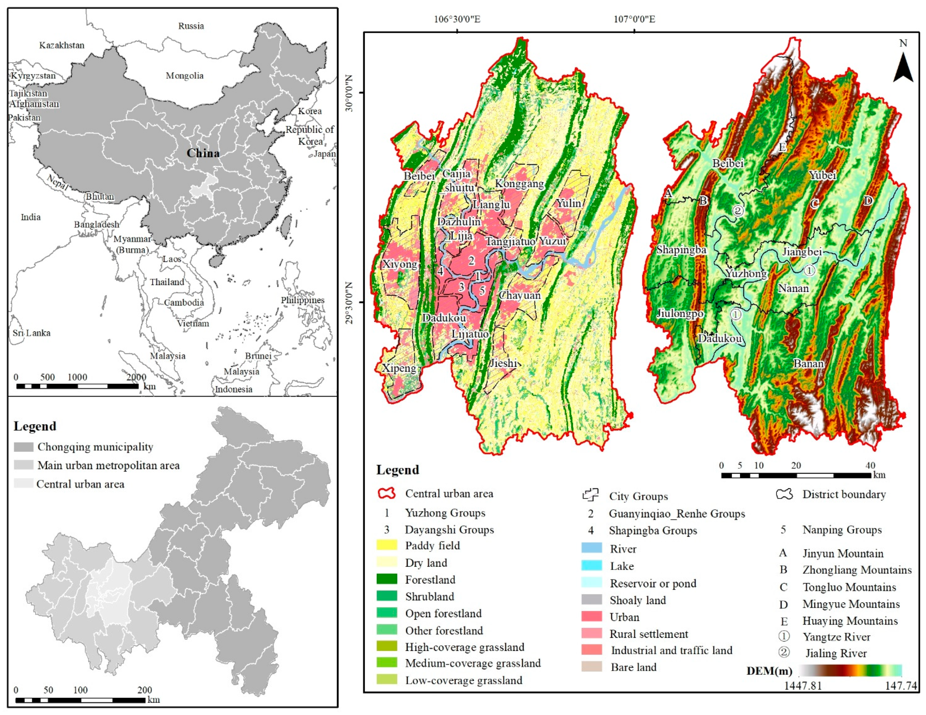
2.1. Study Area

The CUACM (29°8′2″N–30°7′37″N, 106°14′49″E–106°58′26″E), located in southwestern China and the center of the main urban metropolitan area of Chongqing, covers approximately 6.6% of the Chongqing municipality and contains 9 districts (Figure 1). The study area is characterized by a crisscrossing distribution of mountains and rivers, and mainly composed of mountains and hills in the eastern Sichuan parallel ridge-and-valley area. Four parallel mountain ranges, namely, the Jinyun, Zhongliang, Tongluo and Mingyue Mountains, extend from northeast to southwest. The Yangtze River and Jialing River run through the CUACM from west to east. The area has a subtropical humid monsoon climate characterized by hot summers and warm and foggy winters, and the annual average temperature and precipitation total are 18.3 °C and 1199 mm, respectively. According to Chongqing urban master planning in 2007–2020, the CUACM is under a multi-center groups development mode. The urban population more than doubled between 2000 and 2018, surging from 2.97 to 7.92 million, representing 25.53% of the total population of Chongqing in 2018. With the construction of the Chengdu-Chongqing economic circle, the urbanization level increased substantially from 55.27% to 90.51%, and the gross regional domestic product (GDP) increased more than 13-fold [36]. The CUACM plays an important role in the upper Yangtze River economic belt and regional ecological protection.

2.2. Data Sources and Processing

The following datasets were used in this study, including land use types, geomorphological, meteorological, soil, vegetation, distance factors and socioeconomic dataset. The detailed descriptions of the data sources and processing were presented in Table 1.

2.3. Methods

The framework of the methodology established in this study can be divided into five sections (Figure 2). First, the quantitative evaluation of ESs based on the InVEST model. Second, spatial–temporal change trend analysis of ESs by the least-squares regression model. Third, ESs hotspots identification and spatial–temporal heterogeneity analysis. Fourth, the determination of the complex relationships among ESs using spearman coefficients, bivariate Local Indicators of Spatial Association (LISA) and ecosystem services bundles (ESBs). Finally, driving mechanism analysis by GAM.

2.3.1. ESs Evaluation and Validation

Habitat quality as a proxy for the potential of regions in supporting BI was modelled, and it refers to the ability of the ecosystem to provide conditions appropriate for individual survival, reproduction and population persistence [44]. Areas with high habitat quality will better support all levels of biodiversity and have relatively intact structure and function [45]. Habitat quality is a function of each threat’s relative impact and weight, habitat suitability of different land use types and sensitivity to threat factors [46]. The CF of different land use types was estimated by aggregating the amount of carbon stored in aboveground biomass, belowground biomass, soil and dead organic matter [19]. SC can be described as the difference between the potential and actual soil erosion, which is mainly determined by precipitation, soil properties, topography, vegetation coverage and anthropogenic factors, such as agricultural activities [47]. WC was evaluated by the water yield module, which is based on the Budyko curve and annual average precipitation [48]. It was modified by taking the velocity coefficient, terrain index and soil saturated hydraulic conductivity into account [49]. The detailed methodologies for ESs evaluation were described in Table 2.
The vegetation coverage has a significant positive effect in conservation practice to enhance species richness, which is commonly assessed to derive conclusions on a region’s biodiversity [50]. Net primary production (NPP) is defined as the remaining part of the organic substance amount produced by vegetation during photosynthesis and respiration, which is a direct reflection of the CF capability [51]. Therefore, BI and vegetation coverage, CF and NPP were fitted with linear regression to verify the accuracy of the models. The squares of the correlation coefficients (R2) were 0.85 and 0.82, respectively, suggested better goodness of fitting and higher accuracy. The reliability of the SC simulation results was verified by referencing related research of Liu et al. [52]. The simulation results coincided well with the reference estimates, with the correlation coefficient was up to 0.91, which indicated the credibility of the simulation results. The WC was calibrated with observed data in Chongqing water resources bulletin [53]. There was a strong correlation between observed and simulated values, with the average relative error less than 10% and R2 value greater than 0.95. The model validation results showed that the simulated values were reasonable and reliable.

2.3.2. Spatial-Temporal Change Trend Analysis

At grid scale, the least-squares regression model was used to detect the regional differences in ESs change trends [54]. Based on the precision of data, the grid size was selected as 30 m × 30 m. Furthermore, we made the statistics of ESs and their changes at administrative district scale. The least-squares regression model can be expressed as follows:
S l o p e = n i = 1 n x i a i i = 1 n x i i = 1 n a i n i = 1 n x i 2 ( i = 1 n x i ) 2
where slope is the change rate of ES; n is the number of years; xi represents the year i; and ai is the ES in year xi. When slope > 0, ES displays an increasing trend and vice versa. The statistical significance was tested by F-test [24].

2.3.3. ESs Hotspots Identification

ESs hotspots represent statistically significant high-value spatial aggregations [55], and they were identified by the Z-scores and P value test of the Getis–Ord value Gi* based on a distance weight matrix in spatial correlation analysis. Gi* is defined as:
G i * = j = 1 n W i j x j j = 1 n x j
where xj is the property value of factor j; Wij is the spatial weight between factors i and j; and n is the number of factors.
For statistically significant positive Z-scores, the larger the Z-score is, the higher the degree of high-value spatial aggregation. The areas with a confidence level greater than 90% were considered as ESs hotspots [56]. The same ecosystem has the potential to provide multiple ESs. The distribution of multiple ES hotspots could be determined by overlaying the four ESs hotspots [49,57]. The region with four ESs hotspots was defined as a class 4 of ESs hotspots, similarly, class 3, class 2, and class 1 ESs hotspots were identified.
To comprehensively reflect the detailed characteristics of topographic spatial heterogeneity of multiple ES hotspots, terrain niche index (TNI) was calculated by combining slope and elevation [58], and it was classified into ten gradients using the natural breaks classification method. Furthermore, the distribution index was used to reveal the spatial distribution of multiple ES hotspots on TNI gradients. The formulas are as follows:
T = lg [ ( E E ¯ + 1 ) × ( S S ¯ + 1 ) ]
where T is the terrain niche index; E and S are the elevation and slope of the grid cell, respectively; and E ¯ and S ¯ are the average elevation and slope of the study area, respectively.
P = ( S i e S i ) / ( S e S )
where P is the distribution index; Sie is the area of ESs hotspots on the TNI gradient e; Si is the area of ESs hotspots; Se is the area of TNI gradient e; and S is the total area of the entire study area. Generally, greater P values indicate a high distribution frequency of ESs hotspots on a certain TNI gradient. When P > 1, the TNI gradient represents the dominant distribution of ESs hotspots.

2.3.4. Investigating the Complex Relationships among ESs

In order to eliminate the influences of different units and scales, ESs were standardized using a minimum–maximum normalization to obtain comparable and dimensionless data ranging from 0 to 1 [59]. Considering the sensitivity of this standardization to extreme values, the ESs were first transformed by winsorization where ESs with values less than the 5% quantile and greater than the 95% quantile were assigned values of the 5% and 95% quantile, respectively [60,61].
Spearman rank correlation coefficients were used to illustrate the trade-offs and synergies between ES pairs at a regional scale since the ESs data did not conform to normal distribution [62]. The formula is as follows:
r = 1 6 i = 1 n d i 2 n ( n 2 1 )
where r is the correlation coefficient; n is the number of ES pairs; di is the rank difference. When r > 0, there is a positive correlation, which indicates that the paired ESs were synergistic; when r < 0, there is a negative correlation suggesting trade-offs between ES pairs. In accordance with Raudsepp-Hearne et al. [63], the strength of the correlations was described by using the following classification: strong correlation (|r| ≥ 0.5), moderate correlation (0.5 > |r| ≥ 0.3), weak correlation (0.3 > |r| ≥ 0.1) and no correlation (|r| < 0.1). T-test was performed to test for statistical significance [64]. * p < 0.05 was considered statistically significant.
Bivariate local Moran’s I was used to explore the trade-offs (spatial dispersion) and synergies (spatial aggregation) between ES pairs on spatial scale [65]. The formula is as follows:
I i j = x i a x ¯ a σ a j = 1 n ( W i j x j b x ¯ b σ b )
where Iij is bivariate local spatial autocorrelation coefficient; n is the number of grid cells; Wij is spatial weight matrix; xia and xjb are the value of ES a and ES b in grid cell i and j, respectively; and x ¯ a , x ¯ b , σa and σb are the average and variance of ES a and ES b, respectively. The statistical significance of bivariate local Moran’s I was examined by permutation tests; and 999 permutations were used in this study [66]. The significance value for spatial correlation between ES pairs were classified as significant (* p < 0.05), very significant (** p < 0.01), and extremely significant (*** p < 0.001).
Positive spatial autocorrelation was when similar values clustered together on a map, and negative spatial autocorrelation was when dissimilar values clustered together. Therefore, the four cluster types of local spatial autocorrelation generated by bivariate LISA were reclassified as trade-offs and synergies. The high-high and low-low clusters were reclassified as synergies, the high-low and low-high clusters were reclassified as trade-offs.
ESBs can reflect the aggregation and combination of multiple ESs on spatial and temporal scales, which can quantify the complex interactions among multiple ESs. ESBs were identified by K-means clustering algorithm [33]. To minimize the total error sum of squares, the number of initialized repeating runs and iterations were set to 150 and 1000, respectively [11,63]. The optimal number of clusters was determined by the ratio of the between-cluster sum of squares and the total sum of squares. The higher the ratio, the greater the difference between clusters and the smaller the difference within clusters. After series of trials and analysis, when the number of clusters was set to five, the ratios were the highest, which were 80.16%, 81.12% and 80.07% in 2000, 2010 and 2018, respectively. The five ESB types were visualized using petal plots, and the length of each petal represents the average of ESs [23].

2.3.5. ESs Driving Mechanisms

GAM was employed to examine the linear or nonlinear relationships between driving factors and ESs in 5468 grid cells of 1 km × 1 km located across study area using the mgcv package of R [61]. GAM had advantage in developing realistic response curves because it fit non-parametric smoothers to the data without requiring priori specifications to describe nonlinearity [67]. All driving factors entered the GAM as smooth terms. The general expression of the model is as follows:
g ( μ ) = β 0 + x i β + j = 1 n f j ( x i j ) + ε
where g is the link function; μ is the expectation of dependent variable Y; β0 is the intercept term; xi and β are the independent variables and parameters of fixed effects; fj(xij) is non-parametric smoothing functions; and ε is the error term.
Based on the principles of scientificity, representativeness and accessibility, 32 natural environment and socioeconomic factors were selected to build the driving factors database, including: (1) seven geomorphological factors, (2) land use types, (3) NDVI and NPP, (4) four meteorological factors, namely, temperature, precipitation, rainfall erosivity index and reference evapotranspiration, (5) four soil factors, namely, soil types, erodibility, saturated hydraulic conductivity and organic carbon content, (6) five distance factors, namely, the distance to cultivated land, forestland, grassland, waters and construction land, (7) three socioeconomic factors, namely, POP, GDP and NTL, and (8) six policies, namely, CUACM overall urban planning in 2004–2020 (CMOUP), multi-center groups development strategies in Chongqing urban master planning in 2007–2020 (MGDS), regulations on developments and controls of the four parallel mountains (RDCFM), Chongqing ecological function regionalization (CEFR), Chongqing ecological redline (CER), and beautiful landscape city planning in CUACM (BLCP).
The collinearity was detected by the variance inflation factor (VIF) and driving factors with a VIF greater than 5 were sequentially removed [68]. Akaike’s information criterion (AIC) and adjusted determination coefficient (R2adj) were applied to check the goodness-of-fit of the model [69]. The AIC and R2adj of four GAMs between ESs and driving factors were −25,399.34, −21,417.56, −11,355.13, −25,203.94 and 0.869, 0.859, 0.603, 0.666, respectively, suggested good model performance and explanatory power. T-test and F-test were used for categorical and numerical variables, respectively. The statistical significances were classified as significant (* p < 0.05), very significant (** p < 0.01), and extremely significant (*** p < 0.001).

3. Results

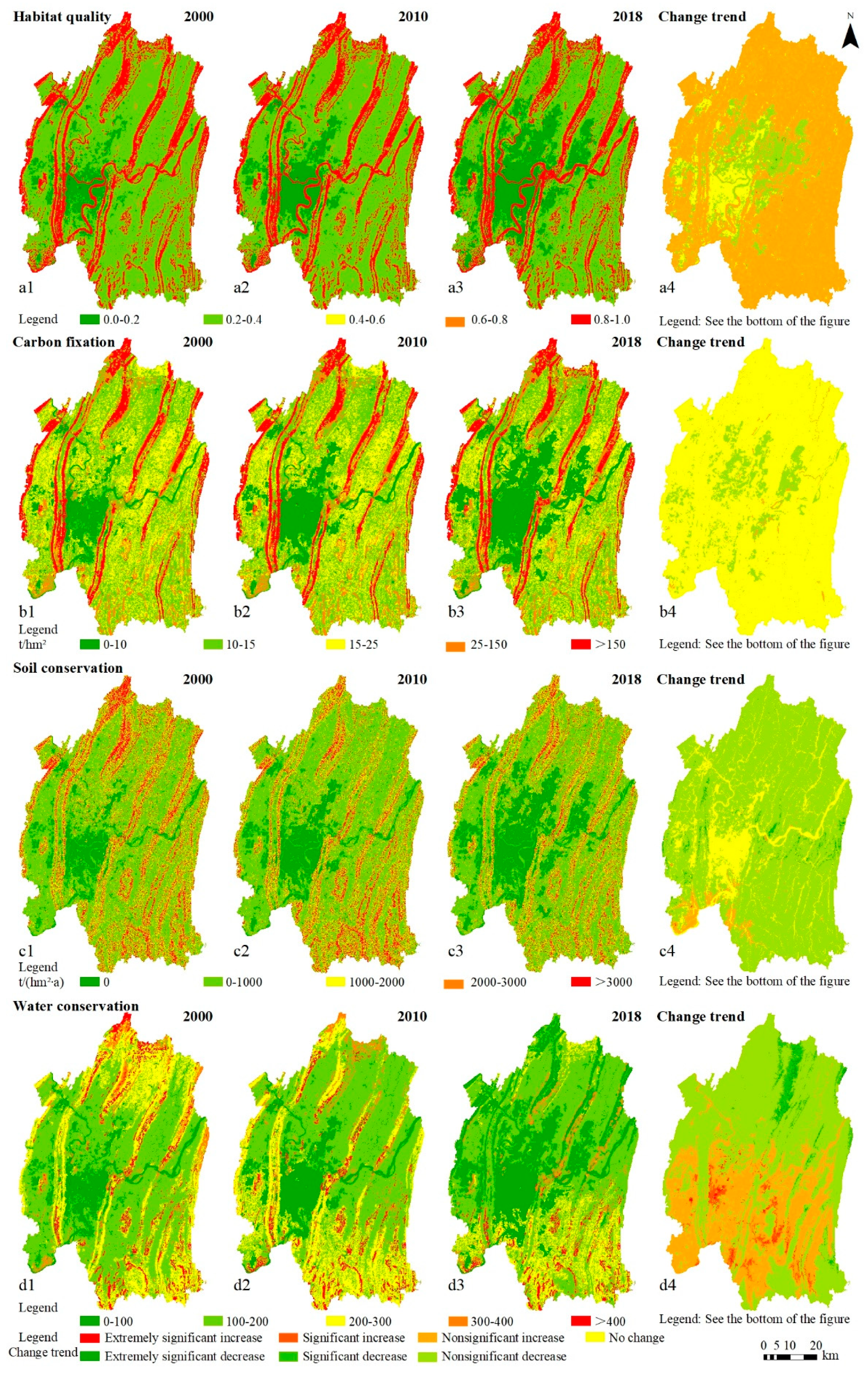
3.1. Spatial Patterns of ESs

All the four ESs demonstrated clear spatial clustering on the study area and exhibited different change trends. High BI areas with high habitat quality were concentrated in Jinyun, Zhongliang, Tongluo, Mingyue, Huaying and southeastern mountainous areas (Figure 3(a1–a3)). The Yangtze River, Jialing River and other water bodies also had higher BI. The BI displayed a decreasing trend, with the habitat quality index declining from 0.5 to 0.45 during 2000–2018. Areas with decrease trends were mainly distributed in peri-urban expanded regions, and most of which (99.51%) was nonsignificant decrease areas (Figure 3(a4)). Similar to BI, CF also showed a high spatial pattern in mountainous areas (Figure 3(b1–b3)). The change of CF was not obvious overall, with a trend of decrease first and then increase. In most of the study area (89.42%), CF remained unchanged. Additionally, a similar nonsignificant decreasing trend was observed in peri-urban expanded regions (Figure 3(b4)). The high values of SC were not evenly distributed in mountainous areas (Figure 3(c1–c3)), showing obvious topographic heterogeneity. There was a trend of decrease in SC from 1289.56 t/hm2 to 921.90 t/hm2. Approximately 81.36% of the study area showed a decreasing trend in SC, of which 97.82% decreased was nonsignificant (Figure 3(c4)). The high values of WC were mainly located in mountainous areas, which was profoundly influenced by precipitation (Figure 3(d1–d3)). The average WC depth decreased from 192.43 mm in 2000 to 141.79 mm in 2018. The areas with decreasing WC accounted for 65.20%, and were mainly found in mountainous areas and the northern half of the study area, whereas the increases occurred in the southern portion (Figure 3(d4)). Additionally, most of the changes were nonsignificant. The change trend of WC from 2000 to 2018 had good consistency with precipitation change. Due to the frequent interference of human activities, all ESs in urban areas were extremely low.
At the administrative districts scale, Beibei had the highest level of BI, followed by Banan and Yubei (Figure 4a). The highest average values of CF were also detected in Beibei, followed by Shapingba, Jiulongpo and Yubei (Figure 4b). The highest average SC and WC occurred in Banan, followed by Beibei and Yubei (Figure 4c,d). All ESs in Yuzhong were the lowest and far lower than those in other districts. It is worth mentioning that there were some increases in CF in Nanan, Yubei and Yuzhong. In addition to this, the general trends of ESs for all districts were descending. The maximum reductions of BI and CF were observed in Jiangbei. The dramatic decreases in SC and WC were observed in Beibei, Yubei and Jiangbei.

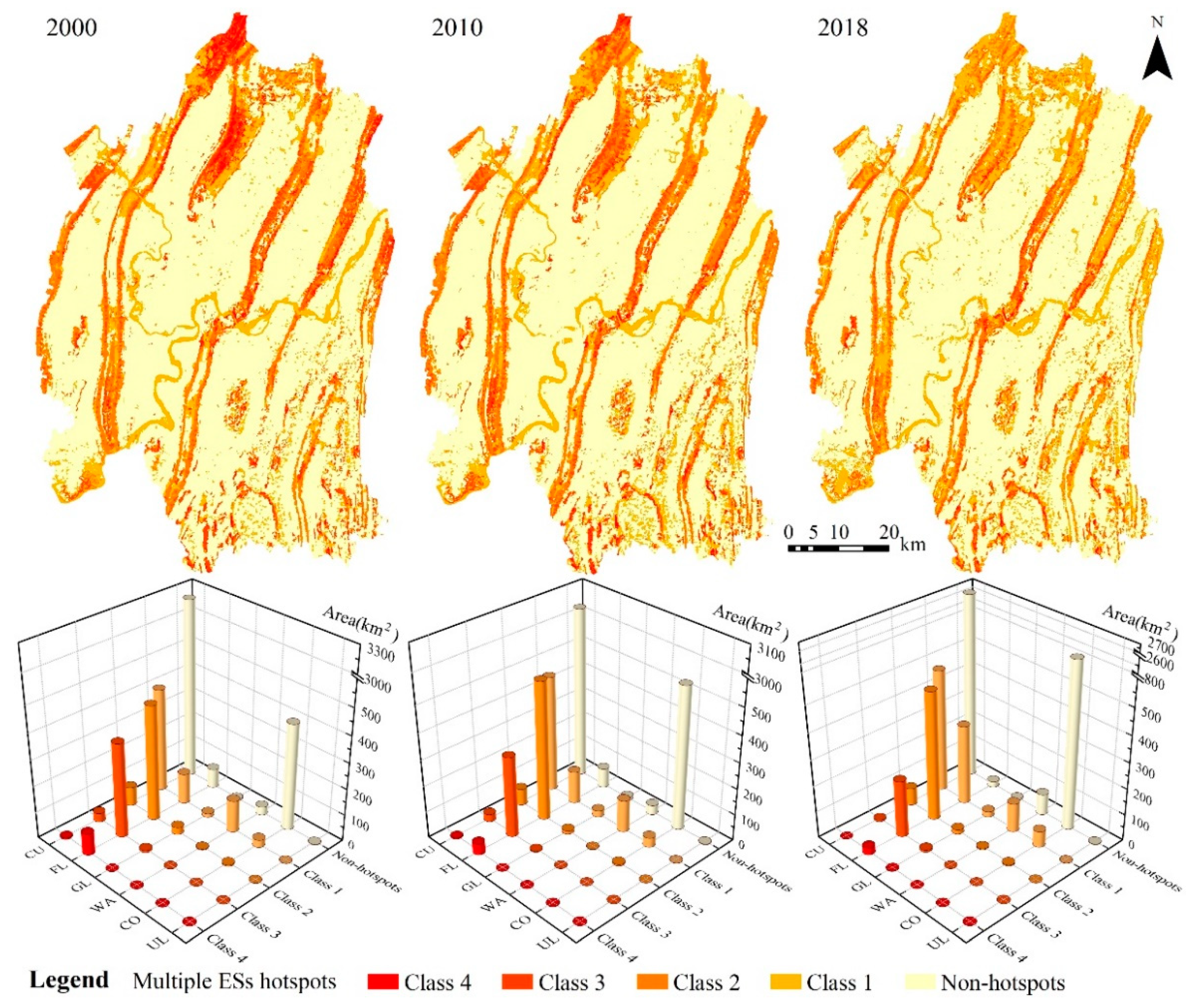
3.2. Spatial Heterogeneity of ES Hotspots

The results of hotspots analysis suggested clear characteristics in temporal and spatial distribution for multiple ES hotspots (Figure 5). During 2000–2018, the total area of multiple ES hotspots exhibited a slightly increasing tendency, with the area proportion increased from 31.55% (1726.45 km2) to 33.19% (1816.22 km2). Specifically, increases in class 1 ES hotspots were strongest. Class 2 ES hotspots also behaved a general increasing trend of increased first and then decreased. In 2018, the proportion of both to all ES hotspots reached as high as 53.46% and 32.16%, respectively. Class 3 and class 4 ES hotspots had a tendency to decrease, accounting for only 12.80% and 1.58% of all ES hotspots in 2018, respectively.
There was considerable variability in ESs delivered by different land use types, which led to the spatial heterogeneity of multiple ES hotspots (Figure 5). Class 1 ES hotspots occurred mainly in cultivated land, forestland and waters, with the average proportion of 55.41%, 21.78% and 15.23%, respectively. Class 2 ES hotspots were mainly composed of forestland and cultivated land, covering 83.68% and 11.76%, respectively. The average contribution of forestland to class 3 ES hotspots reached 91.12%. Although the area of forestland showed a decreasing trend, the area proportion showed an increasing trend, which was caused by the decrease of class 3 ES hotspots. The most predominant land use type that composed class 4 ES hotspots was forestland, accounting for 94.10% in 2000, 91.90% in 2010 and 94.07% in 2018. The non-hotspots were primarily covered by cultivated land and construction land. Generally, forestland was a major contributor to ESs and also had a significantly higher area proportion of multiple ES hotspots compared to other land use types. Among them, the average area proportion of class 1, 2, 3 and 4 ESs hotspots were 17.09%, 45.42%, 27.48% and 4.69%, respectively. The area of grassland was small, but it had an important role in ESs supply, second only to forestland. During 2000–2018, multiple ES hotspots accounted for an average of 84.02% of grassland. The average area proportion of multiple ES hotspots of waters ranged from 80.24% to 58.70% in a decreased trend. Additionally, average 70.27% of waters was class 1 ES hotspots. Most of unused land, cultivated land and construction land were non-hotspots, which accounted for averages of 70.25%, 84.70% and 92.86% of such kinds of land use, respectively.
The distributions of multiple ES hotspots had distinct spatial heterogeneity in different TNI gradients (Figure 6). In the 1st TNI gradient and high TNI gradients (6th–10th), the average distribution index of class 1 ES hotspots were greater than 1, indicating that it was primarily located in two parts of the study area: water areas with low altitude and slope, such as the Yangtze River and Jialing River, and the transition zone between mountainous areas and flat areas with medium-high altitude and slope. The distribution index of class 1 ES hotspots tended to decrease in the 1st TNI gradient over time, while it increased in the 6th to 10th TNI gradients. Class 2 and class 3 ES hotspots were mainly distributed in high TNI gradients (6th–10th), with average distribution index of 2.18 and 2.52, respectively. In the 10th TNI gradient, an upward trend in distribution index was observed of class 2 ES hotspots, while the trend of class 3 ES hotspots was downward during 2000–2018. The distribution index of class 4 ES hotspots presented a tendency to increase with an increase in TNI gradients, especially after the 7th TNI gradient. Although the distribution index showed a decreasing trend in the 10th TNI gradient during 2000–2018, it was still much larger than that in other gradients, which indicated that the mountainous areas with high altitude and steep slope were always the predominant distribution areas of four ES hotspots.

3.3. Spatial-Temporal Trade-Offs and Synergies between ES Pairs

During 2000–2018, the significant positive correlations (Spearman coefficient: r > 0; p < 0.001) were found between all ES pairs in the entire study area (Figure 7). It demonstrated that all six pairs of ESs exhibited synergistic relationships. In 2000, there was a strongest positive correlation between BI and WC. The relationship between SC and WC was also strong synergistic. In 2010, the highest positive correlation was observed between BI and CF. Additionally, WC also had strong positive correlation with BI and SC. In 2018, the synergistic relationship between BI and CF remained strongest. Strong positive correlations were also found between SC with BI and CF. In addition, the correlation coefficients among BI, CF and SC showed a tendency to increase during 2000–2018, which indicated that the degree of synergies were gradually enhanced. With the relationship between BI and WC changed from strong correlation to weak correlation, the synergy was diminished. The relationships between WC with CF and SC showed a general weakening trend of slightly enhanced first and then weakened.
There were obvious differences in spatial distributions of trade-offs and synergies between ES pairs (Figure 8). For BI and CF, synergies were always the dominant relationship in the study area, with the area proportion ranging from 68.53% to 68.18%. Among them, significant synergy accounted for average 59.20%, which was mainly distributed in the flat areas between mountains. The extremely significant synergy showed a gradually increasing trend, with an average area proportion of 33.04%, which were mainly concentrated in the high-high and low-low clusters, i.e., mountainous areas and urban central areas. The extremely significant trade-offs accounted for 4.13% of the study area and were spatially aggregated in waters, especially in Yangtze River and Jialing River. For BI and SC, synergies and trade-offs accounted for average 35.13% and 8.94%, respectively. The synergies were found mainly in the intermountain flat areas and scattered in Jinyun, Zhongliang, Tongluo and Mingyue Mountain. The trade-offs were mainly distributed in Yangtze River and Jialing River, and also observed in Qiaoping mountain and southeastern mountainous areas. For BI and WC, the area of synergies was comparable to trade-offs, accounting for 27.33% and 20%, respectively. The extremely significant synergies were distributed in two dominant parts: one located in mountainous areas and the other in urban areas. During 2000–2018, the former exhibited a downward trend, while the latter showed the opposite trend. The trade-offs tended to increase, and the most dramatic increase was observed in significant trade-offs, which located in some mountainous areas and southeastern areas. The extremely significant trade-offs still mostly occurred in Yangtze River and Jialing River. Apart from Yangtze River and Jialing River changing from trade-offs to synergies, the trade-offs and synergies between CF with SC and WC followed a spatial pattern similar to the relationships between BI with SC and WC. In addition, similarity was also observed in general change trends. For SC and WC, the synergies were dominated by the extremely significant synergies, which mainly occurred in urban areas, mountainous areas with an elevation of 200~700 m and a slope of 5~15°, as well as waters such as Yangtze River and Jialing River. Both the area of synergies and trade-offs showed the same increasing trend, but the magnitude of changes was most pronounced in significant trade-offs. The significant trade-offs increased by 441.40 km2, which were mainly located in some mountainous areas and southeastern intermountain hilly and flat areas.

3.4. ES Bundles among Multiple ESs

Five ESBs were determined by K-means cluster analysis (Figure 9). In 2000, ESB1 was spatially clustered in Jinyun, Zhongliang, Tongluo, Mingyue, Huaying and southeastern mountainous areas with an average elevation of 535.83 m and slope of 9.57°. It was predominantly covered by the highest proportion of forestland (92.93%), occupying 6.30% of the study area. ESB1 was especially characterized by the highest BI, CF, SC and the second-highest WC, which was only 0.07 lower than that of ESB2. ESB2 were interlaced with ESB1, mainly distributed in mountainous areas with an average elevation of 515.78 m and slope of 6.45°, and mostly covered by forestland (87.84%). It showed the highest WC, the second-highest BI and CF, and moderate SC. ESB3 was observed in the piedmont transition zone between mountainous and flat areas with an average elevation of 436.57 m and slope of 7.29°, contained 94.51% of cultivated land. SC was dominant in ESB3 and second only to that of ESB1. The mean values of BI and CF were below the regional averaged values, whereas the mean value of WC was slightly above the regional average value. Covering 63.45% of the study area, ESB4 were widely spread in the intermountain flat areas, the trough and valley at the top of anticline mountains, as well as water areas. The land use pattern of this bundle was characterized by larger cultivated land ratios (92.24%), followed by waters (4.43%). ESB5 was characterized by dense urbanization and concentrated in urban areas, with the proportion of construction land of 90.58%. All ESs in this bundle were at the lowest level.
In 2010, ESB1 was increased and clustered in mountainous areas with an average elevation of 520.04 m and slope of 7.46°. It supplied the highest BI, CF, WC and the second-highest SC. Different from ESB2 in 2000, ESB2 were mainly distributed in waters, such as the Yangtze River and Jialing River, with an average elevation of 281.64 m and slope of 3.26°. The proportion of waters in this bundle was up to 66.66%, followed by forestland (4.43%). ESB2 provided a relatively higher BI and lower CF, SC and WC. The characteristics and distributions of ESB3, ESB4 and ESB5 were similar to those in 2000. The slight difference was that ESB3 showed the highest SC compared to other ESBs.
In 2018, ESB1 contributed strongly to WC, provided a relatively higher BI and CF, and moderate SC. It was located in mountainous areas with an average elevation of 489.40 m and slope of 6.59°, mainly consisting of forestland (79.34%) and grassland (10.77%). ESB2 was spatially clustered in mountainous areas with an average elevation of 538.99 m and slope of 7.97°, covered mainly by forestland (92.36%). It was characterized by the highest BI and CF, the second-highest SC, which was second only to that of ESB3. However, the mean value of WC was below the regional averaged value. ESB3, ESB4 and ESB5 had quite similar distributions and combinations of ESs with those in 2000 and 2010. Notably, as urban sprawl, the area of ESB5 presented a dramatic increasing tendency from 444.08 km2 to 947.33 km2. This increase mainly occurred in new cities groups and the periphery of the original cities.

4. Discussion

4.1. Exploring the Driving Mechanisms of ESs

ESs were deeply influenced by natural environment, socioeconomic and policies factors [33]. Different from previous studies [70,71], we quantitatively investigated linear or nonlinear relationships between ESs and driving factors based on GAM. Although relevant studies had elaborated that land use was the primary driver of ES changes, most of the results were only presented in the form of qualitative description [32,71]. There was particularly a lack of focus on political drivers of ESs [30]. We included land use types and policies as fixed effects in GAM, and the parameter estimates illustrated the influence of different independent variables on ESs (Table 3). Regarding the land use types, BI had extremely significant strong positive correlations with forestland, grassland and waters, the parameter estimates were up to 0.939, 0.896 and 0.878. CF were most enriched in forestland, followed by grassland. Strong and moderate positive correlation was found between WC with grassland and forestland, respectively. These parallels the majority of previous findings that, forestland and grassland can not only support high biodiversity by providing resources and habitats for species, but also provide high carbon sequestration and had low runoff potentials that contributed greatly to water conservation [61,72]. However, SC was shown to be weakly correlated with land use types. This may be because SC was more strongly affected by geomorphological factors, which was confirmed by Baró et al. [33].
The effects of policies on ESs, although significant, appear to be modest. The RDCFM, CER and BLCP had weak positive effects on BI, CF and SC, while they had weak negative effects on WC (Table 3). Two possible reasons may be able to account for these. First, lack of scientific and sufficient information on ESs to serve as comprehensive evaluation criteria for delineation of protected areas resulted in the co-existence of over-protected and conservation gaps in policies [73]. Second, the policies were formulated based on the conditions at a certain time, while ecosystems were dynamic, and follow changes in the natural and socioeconomic environment [74]. Despite effectiveness limitations and time lag of policies, our results indicated that policies had positive effects on the BI, CF and SC. However, WC was mainly determined by climate factors and fluctuated with precipitation variation. The study of Cui et al. [70] had demonstrated that the spatial change of WC was consistent with that of precipitation.
The results of GAM for ESs revealed the relative effect and importance of various driving factors, and the smooth functions showed the linear or nonlinear relationships between ESs and driving factors. The distance to forestland was the main influencing factor for BI with the highest F-value of 17.05, followed by the distance to cultivated land (F = 12.51) and elevation (F = 9.174) (Table S1, Figure 10). There was a decreasing trend generally in BI with the increasing distance to forestland. The observed appearance of the crest was closely related to waters with a higher BI, which were crisscrossed and interlaced with mountains. The CUACM was characterized by northeast–southwest trending parallel mountain ranges and west–east trending rivers, interspersing with flat valleys and urban groups. The complex spatial mosaic of landscapes resulted in a strongly nonlinear relationship between BI and the distance to cultivated land, waters and construction land. BI showed a general increasing trend of decrease first and then increased with increasing elevation and TNI. This was because waters were primarily located in the low TNI with low altitude and slope. Relevant studies had shown that waters created diverse and stable habitats for waterfowl and fish to forage, refuge and breed [75]. In addition, the same relationships were also observed between BI with NPP and soil organic content. NDVI had a very significant positive effect on BI, and an estimated degree of freedom equal to one confirmed the linear relation. There was a general negative relationship between BI and precipitation. One likely explanation for this may be that a large amount of precipitation had the potential to induce geological disasters in mountainous areas, which had a certain negative impact on BI. A similar negative correlation had been discovered in a study of the Yangtze River Economic Belt [76]. BI decreased nonlinearly with increasing population density. The ever-increasing population led to an expanding demand for natural resources and produces [77], which caused dramatic interference with BI [78].
The strongest effects on CF were soil organic content (F = 113.68), distance to forestland and grassland (Table S1, Figure S1). CF showed an extremely significant positive correlation with soil organic content, which had been suggested to be one of the main determinants of plant species distributions and ecosystem functioning [79]. As the distance to forestland increased, CF was overall decreased. As it can be observed, crest clearly appeared because grassland and cultivated land had a certain potential for carbon sequestration [80]. Consistent with previous studies [81], forestland was the major component of carbon pool in the study area, with a contribution of 76.92%. Thus, CF showed a trend of decreased first and then increased with increasing distance to grassland. The higher elevation, TRI and TNI, the higher forestland coverage and the higher CF. Affected by the trend of the mountains from northeast to southwest, the area proportion of forestland was relatively higher on east and west slope. The CF was fluctuated with aspect variation and peaked approximately at 100° and 275°. The smooth fitting curve between CF and TPI appeared a V-shape. The areas, with the TPI equal to zero, were mostly flat areas, such as rivers and lakes, which had the lowest CF. The higher or lower the TPI, the closer it was to the ridge or valley and the higher the CF. The CF had a very significant linear increase trend with increasing NDVI, and it also had a general tendency to increase with NPP. The result was in line with recent findings in which vegetation coverage had a notable positive impact on NPP, and higher NDVI significantly improved CF [24,57]. Similar to that of BI, CF was negatively correlated with precipitation. Due to the complex spatial pattern of landscapes, CF had nonlinear relationships with the distance factors. CF exhibited a diminishing trend with the increased in population and GDP. Generally, in areas with a higher population and GDP, urbanization was usually higher. The demand for urban land had gradually increased, and a large amount of ecological land was occupied, which may be the major causes for CF loss [2].
Geomorphological factors were the dominant factors for SC, such as TPI (F = 1313.929), TNI and slope (Table S1, Figure S2). There was a negative and saturating relationship between SC and TPI. Specifically, SC decreased rapidly with increasing TPI when TPI was less than zero, whereas there was little change in SC when TPI was greater than zero. It means that the closer the valley, the higher the SC. According to Tsaaer et al. [82], the valleys were considered to be favorable sites for soil deposition, with large forest area and relatively lower soil loss. The areas with higher TNI and steep slope usually had higher vegetation coverage, the actual soil loss was considerably lower than potential soil loss, resulting in a higher SC [83]. SC displayed a tendency of increased first and then decreased with elevation. When the elevation was greater than 700 m, the higher the elevation, the higher the vegetation coverage, which can effectively intercept precipitation and reduce soil erosion, resulting in a decrease in sediment deposition from upstream, and a downward trend in SC [52]. Influenced by the mountain range trend, SC exhibited a double hump-shaped relation with aspect, peaking at about 90° and 270°. The CF had a positive linear correlation to NDVI and precipitation, and tended to nonlinearly increase with increasing NPP and soil organic content. The higher the vegetation coverage, the higher the NDVI and NPP, the thicker the litter layer, the more developed root systems, the higher the soil organic content, which can prevent soil erosion from rain splash [24], resulting in a decrease in actual soil loss and an upward trend in SC. The precipitation had the most direct positive effect on the potential soil loss, resulting in a higher SC. In general, the closer to the forestland and the further away from the construction land, the higher the SC.
Our findings suggest that WC was mainly controlled by precipitation (F = 472.458), which was in accordance with previous studies [70] (Table S1, Figure S3). Generally, in areas with a higher precipitation, water yield was usually higher, which led to higher WC. WC was also influenced by other factors, once the resistance of the controlling ability of precipitation for WC was broken, WC decreased significantly. Singh et al. [84] also corroborated a high rainfall did not guarantee a high WC in a region as it depends on variety of factors. WC increased linearly with elevation and nonlinearly with TNI. When the slope was less than 30°, WC increased rapidly with increasing slope, whereas there was a slightly decreased in WC when slope was greater than 30°. The higher the TNI with higher altitude and slope, the higher the vegetation coverage. The dense canopy had the ability to trap precipitation [24], the thick litter layer and developed root systems made more water infiltrated into the soil [26], and thus there will be an increase in WC. However, as soon as the slope exceeds 30°, water holding capacity strongly decreased, resulting in reduction of WC. Thus, there was lower WC on the ridges with steep slopes, while valleys had the highest WC. NDVI, NPP and soil organic content had extremely significant positive effects on WC, although slightly decreased or saturated at the highest values. Plants can not only absorb and store some precipitation, but also increase regional precipitation through plant transpiration [49]. The higher the soil organic content, the higher the water holding capacity. WC showed a fluctuating downward trend with the increasing distance to forestland while increased with the distance to waters, which was affected by the complex spatial pattern of mountains and rivers. Meanwhile, WC showed a general decreasing trend of decreased first and then increased or unchanged with the distance to grassland and cultivated land. WC had a linear positive correlation with the distance to construction land, whereas had an opposite correlation with population and GDP. With the increase of human activity intensity, a large amount of natural vegetation was converted into impervious surface [57], which directly led to the decrease of WC.

4.2. Scale Effect of ESs and Their Complex Interactions

Our study examined spatial-temporal heterogeneity and complex interactions of four key ESs, i.e., BI, CF, SC and WC. These ESs not only can reflect the key ecological problems facing the CUACM [85], but also have great contributions to regional welfare and sustainable development [24]. At grid scale, there was obvious spatial agglomeration of ESs in mountainous areas. Numerous studies have proved that multi-dimensional topographic factors in mountainous areas not only controlled the spatial distribution pattern of solar radiation and precipitation, but also affected the spatial heterogeneity of soil properties [86,87]. Characterized by diverse vegetation types and complex vegetation structures, mountainous areas not only provided high CF, but also provided various suitable habitats for species [88]. The mountainous areas, with high elevation, steep slope and high vegetation coverage, had a high potential soil erosion, low actual soil erosion and a low runoff that contributed greatly to SC and WC [61]. At the administrative districts scale, ESs were relatively higher in Beibei, Banan and Yubei, and drastically decreased in Jiangbei, which were closely related to regional vegetation coverage and urbanization development. Banan, Beibei and Yubei had relatively high average vegetation coverage, which were 0.86, 0.79 and 0.78, respectively. In 2008, according to CEFR, Banan, Beibei and Yubei had been designated as important ecological barriers of the study area. Affected by the development of Liangjiang New Area and the rapid expansion of urbanization, the ecological land in Jiangbei district was occupied by construction land, which directly led to the reduction of ESs. This was consistent with the research of Wang et al. [2], showing dramatically decreased in ESs with urban land expansion. It is worth noting that the spatial congruence of WC was relatively low from 2000 to 2018, which was mainly affected by the interannual variation of precipitation and potential evapotranspiration. Although the precipitation decreased first and then increased (992.89 mm, 980.42 mm and 1126.55 mm), the magnitude of its change did not exceed the increases in evapotranspiration (778.08 mm, 769.09 mm and 1364.77 mm). Growing studies has been discussing that the change of WC is not completely determined by land use change, but dominated by regional climate change and human activities [70,89]. At present, most studies have primarily focused on the spatiotemporal pattern analysis of ESs [90], but the scale-dependent effects have usually been ignored, such as land use and topographic heterogeneity. The spatiotemporal heterogeneity of ESs at different scales can be more clearly characterized by hotspots identification [2]. In our study, it can be clearly seen that multiple ES hotspots were mainly composed of forestland and distributed in high TNI with high altitude and steep slope, which proved the spatial-temporal patterns of ESs mentioned above.
ESs were dependent on dynamic processes that act and interact at different scales. Therefore, the interactions between ES pairs had obvious scale effects. Yang et al. [28] found that the degree of trade-offs between ESs tended to weaken gradually as the scale increased, and there were even signs that it would turn into synergies. Again, remarkably similar results were obtained in our study. In the entire CUACM, there was a positive relationship within ESs, indicating synergy or at least no conflicts. A possible explanation was that they shared common driving factors, such as land use, TNI and NDVI. Specifically, the forestland located in high TNI with high elevation, slope and NDVI not only provided suitable habitats for species, but also had the highest potential for CF [81]. The dense canopy, thick litter and developed root systems had an effective capability of rainfall interception, slope stability, and soil and water conservation [24]. However, there was distinct spatial heterogeneity in trade-offs and synergies between ES pairs at grid scale. This can be explained in two ways; on one hand, the natural and social driving factors had distinct geographical differences, on the other hand, each ES had different dominant driving factor. For example, SC exhibited a strong dependence on geomorphological factors, while WC was extremely sensitive to meteorological factors [70]. Bivariate LISA and ESBs had the potential to objectively divide study areas into different groups and make spatial explicit mapping, which can provide novel insights into the understanding and managing of multiple ESs.

4.3. Implications for ESs Management and Urban Planning

Detecting the complex relationships among multiple ESs was crucial for ecosystem management and urban planning. The spatial concordance and segregation among different ESs hotspots coincided with the formation of different types of ESBs, which can provide guidance for ecological function regionalization. Take 2018 as an example, ESB1 delivered 89.09% of class 4 ES hotspots and 50.95% of class 3 ES hotspots (Figure S4a). The multiple ES hotspots occupied 95.19% of the total area of ESB1 (Figure S4b). ESB2 covered 61.57%, 41.59% and 4.72% of class 2, class 3 and class 4 ES hotspots, respectively, with the proportion of multiple ES hotspots was up to 97.09%. This meant that both ESB1 and ESB2 could support multiple ESs simultaneously, which should be determined as the priority areas for ecological protection to ensure regional sustainable development [2]. ESB3 were mainly consisted of non-hotspots and class 1 ES hotspots, covering 60.72% and 29.77%, respectively. Considering that ESB3 was mainly located in the piedmont transition zone, with high proportion of cultivated land and high SC, land consolidation, reforestation and afforestation were urgently needed to enhance the water and soil conservation efficiencies [3]. ESB4 and ESB5 were primarily covered by non-hotspots, accounting for 82.37% and 92.97%. ESB4 was fringe areas of urban sprawl and provide an important buffering function in ecological environmental protection. Ecological protection and restoration projects using nature-based solutions should be implemented to address regional environmental challenges [91]. In terms of the lowest ESs in urban ecosystems that were in ESB5, the creation and protection of green spaces should be encouraged to relieve ecological pressures, whereas the disordered expansion of cities and the occupation of ecological land for construction should be restricted [33]. For example, as the Yangtze River and Jialing River crossed the urban center, establishing protected greenbelts along the rivers should be considered to reduce human disturbances. The ESBs were consistent with the classification of the major function-oriented zone planning [92], which can provide a theoretical reference for decision-making related to ecological protection and urban development. ESB1 and ESB2 may be considered as prohibited development areas, ESB3 as restricted development areas, ESB4 as prioritized development areas, and ESB5 as optimized development areas.
In general, the ESs synergies areas reflected the realizability of ESs multifunctional management and could be used as the pilot areas to solve trade-offs and encourage the formation of ESBs with more ESs hotspots. In synergy areas with the most ESs hotspots, the original ecosystem and vegetation should be strictly protected. The ESs trade-off areas illustrated the severity of trade-offs and should be the priority areas for ecological restoration. In ESs trade-off areas, different ecological restoration measures should be taken according to the different characteristics of trade-offs. For example, the intensity of development and utilization should be properly controlled to prevent construction land from occupying ecological land with high ESs. Implementing the project of returning farmland to forestland and grassland to increase vegetation coverage and maintain biodiversity are also effective means of regional ESs management.

4.4. Applications of Remote Sensing for ESs Evaluation

Remote sensing has the potential of performing synoptic, spatially continuous, and frequent observations at a wide range of locations [93], which can provide quantitative and spatially explicit thematic data regarding various biophysical characteristics that are often spatialized for ESs evaluation [94,95]. In this study, land use based on Landsat interpretation was used as a necessary input to the InVEST model to evaluate ESs. Land use has been widely used as a dominant proxy for ESs [96], such as forest types and cover are useful to estimate raw materials provisioning [97]. Galbraith et al. [98] stated that forest and other natural areas were positively related to the provision of pollination services. De Araujo Barbosa et al. [99] systematically reviewed the literatures on the evaluation of different ESs using remote sensing and pointed out that land cover was the most important proxy variable in all ESs assessments, followed by NDVI. NDVI was taken as an important parameter of cover-management factor in SC evaluation in this study. Extensive studies have demonstrated that vegetation indices derived from remote sensing inversion are an increasingly major data source for ESs evaluation [99]. For example, net primary production can be directly assessed by remote sensors such as MODIS [95]. It is proved that the vegetation indices based on remotely sensed spectral characteristics can also respond to different biodiversity conditions and serve as the basis for cultural services evaluation [18,100]. The geomorphological data obtained from ASTER GDEM V2 digital elevation model was also the key remote sensing information for BI, SC and WC evaluations in this study, as mapping topographic heterogeneity was helpful to reveal the possibility of providing biological refugia and the potential of soil and water loss [101]. Various remotely sensed information can also be used in combination as proxies for kinds of variables which in turn can be used as proxies for ESs [99,102]. Integrating land use, vegetation indices, meteorological, geomorphological, soil characteristics and other reference factors, we assessed BI, CF, SC and WC by InVEST model.
Generally speaking, remote sensing can be used to evaluate ESs in three different ways: direct and indirect measures and in combination with ecosystem models. Most provisioning services are tangible goods that can be quantified by the direct use of remotely sensed radiation information [103]. For example, the production capacity of agricultural and forestry ecosystems can be quantified based on satellite-derived chlorophyll measurements [96]. Since the regulating services are derived from complex ecological functions or processes, they are primarily assessed based on proxy variables reflecting various ecosystem conditions [104]. Taking climate regulation services as an example, it can be estimated by the net ecosystem exchange of CO2 flux, which can be quantified using biomass as proxies [99,105], just as we evaluated CF. Cultural services arise from people’s perception of the natural phenomenon and environment, which are often evaluated by comprehensively considering biophysical characteristics of ecosystems and beneficiaries’ perception [106]. The combination of remotely sensed inversion data in a multi-agent modelling environment has the potential to provide necessary indicators for cultural services evaluation [99,107]. Supporting services are necessary for the maintenance of ecosystems and the production of all other ESs, which are usually estimated by related proxy variables [108]. Maintaining animal and plant diversity is one of the most important supporting services, which can be indirectly evaluated by remote sensing-based habitat mapping, individual spatial distribution mapping, spectral diversity, etc. [109]. In this study, habitat quality was assessed by the InVEST model, and the dimensionless relative value of 0–1 could be used as a surrogate to quantify biodiversity [61]. Although various methods and indicators have been developed to quantify and map ESs, there are still some limitations in the assessment of some ESs, such as cost-intensive and time-consuming [82]. Therefore, considering the main ecological problems faced by the study area and the relative importance of ESs to human well-being, four key ESs were evaluated in this study. Limited by the accessibility and availability of data, there was some inconsistency in the precision and resolution of the dataset, which had become a common problem in ESs evaluation [49].

5. Conclusions

This study demonstrated the effectiveness of the integrated method of InVEST model, the least-squares regression model and hotspots analysis for ESs assessment, spatial–temporal variation and hotspots identification. Based on spearman correlation coefficients, bivariate LISA and K-means clustering, the complex interactions among multiple ESs were detected. GAM was used to discuss the linear or nonlinear relationships between ESs and driving factors. The results showed that: (1) BI, SC and WC displayed decreased trends, while CF tended to remain basically unchanged. High values of ESs were concentrated in mountainous areas, especially in Jinyun, Zhongliang, Tongluo, Mingyue, Huaying mountains. In addition, the Yangtze River, Jialing River and other water bodies also had higher BI. At administrative districts scale, there were relatively higher ESs in Beibei, Banan and Yubei, and the dramatic decreases were observed in Jiangbei, which were closely related to regional vegetation coverage and urbanization development. (2) ES hotspots had distinct spatial heterogeneity in different land use types and TNI gradients. From the land use types perspective, forestland and grassland were major contributors to ESs, with the average area proportion of multiple ES hotspots accounting for 94.68% and 84.02%, respectively. Generally, the distribution index of multiple ES hotspots presented a tendency to increase with an increase in TNI gradients, which indicated that ESs hotspots were predominantly distributed in mountainous areas with high altitude and steep slope. (3) In the entire study area, all six pairs of ESs exhibited synergistic relationships. The correlation coefficients among BI, CF and SC showed a tendency to increase while the synergies between WC and other ESs were diminished. At grid scale, the synergies were mainly concentrated in the high-high and low-low clusters, i.e., mountainous areas and urban central areas. Five ESBs were determined according to the aggregation of multiple ESs on spatial and temporal scales, which can provide theory supports for land management decision-making and urban planning. (4) ESs were primarily driven by natural environment and socioeconomic factors. Land use types had profound impacts on BI and CF; in particular, forestland and grassland showed a clear positive affect. SC was mainly determined by geomorphological factors, while WC was more likely to be explained by precipitation. The unique and crisscrossing landscapes of mountains and rivers resulted in a strongly nonlinear relationship between ESs and the distance factors. Furthermore, policy factors were confirmed to have a certain positive effect on ESs. This study not only provides a scientific basis for the maximization of ESs benefits and multi-objective collaborative management, but is also beneficial to realize the coordinated and sustainable development of regional urban expansion and ecological environment.

Supplementary Materials

The following are available online at https://0-www-mdpi-com.brum.beds.ac.uk/article/10.3390/rs13214248/s1, Table S1: Hypothesis test results of generalized additive model fitting, Figure S1: Smoothing functions of the covariate terms for carbon fixation GAM showing the effect of driving factors, Figure S2: Smoothing functions of the covariate terms for soil conservation GAM showing the effect of driving factors, Figure S3: Smoothing functions of the covariate terms for water conservation GAM showing the effect of driving factors, Figure S4: Area proportion of ecosystem services bundles (ESBs) in different ESs hotspots (a) and area proportion of multiple ES hotspots in different ESBs (b) in 2018.

Author Contributions

Conceptualization, F.W. and X.Y.; methodology, F.W., L.Z., S.L., M.Z. and D.Z.; software, F.W., L.Z. and M.Z.; formal analysis, F.W.; data curation, L.Z.; writing—original draft preparation, F.W.; writing—review and editing, X.Y.; visualization, F.W.; supervision, X.Y. All authors have read and agreed to the published version of the manuscript.

Funding

This research was funded by the National Natural Science Fund of China, grant number 52178031, the Scientific and Technological Project of Chongqing Housing and Urban-Rural Development Commission, grant number 20C01512 and the Key Consulting Projects of Chinese Academy of Engineering, grant number 2020-CQ-X2-5.

Institutional Review Board Statement

Not applicable.

Informed Consent Statement

Not applicable.

Data Availability Statement

The data presented in this study are available on request from the corresponding author.

Conflicts of Interest

The authors declare no conflict of interest.

References

  1. Dirzo, R.; Young, H.S.; Galetti, M.; Ceballos, G.; Isaac, N.J.B.; Collen, B. Defaunation in the Anthropocene. Science 2014, 345, 401–406. [Google Scholar] [CrossRef] [PubMed]
  2. Wang, J.; Zhou, W.; Pickett, S.T.A.; Yu, W.; Li, W. A multiscale analysis of urbanization effects on ecosystem services supply in an urban megaregion. Sci. Total Environ. 2019, 662, 824–833. [Google Scholar] [CrossRef] [PubMed]
  3. Zhang, Y.; Liu, Y.; Zhang, Y.; Liu, Y.; Zhang, G.; Chen, Y. On the spatial relationship between ecosystem services and urbanization: A case study in Wuhan, China. Sci. Total Environ. 2018, 637–638, 780–790. [Google Scholar] [CrossRef] [PubMed]
  4. Millennium Ecosystem Assessment. Ecosystems and Human Well-Being; Island Press: Washington, DC, USA, 2005. [Google Scholar]
  5. Bennett, E.M.; Peterson, G.D.; Gordon, L.J. Understanding relationships among multiple ecosystem services. Ecol. Lett. 2009, 12, 1394–1404. [Google Scholar] [CrossRef] [PubMed]
  6. Wang, C.; Zhu, J.; Zheng, T.; Yan, Y.; Xu, S. Ecosystem services for a sustainable future—A review of the 10th ecosystem services partnership world conference. Acta Ecol. Sin. 2019, 39, 8193–8199. [Google Scholar]
  7. Convention on Biological Diversity. Aichi Biodiversity Targets. Available online: https://www.cbd.int/sp/targets/ (accessed on 28 December 2020).
  8. Schmeller, D.S.; Bridgewater, P. The Intergovernmental Platform on Biodiversity and Ecosystem Services (IPBES): Progress and next steps. Biodivers. Conserv. 2016, 25, 801–805. [Google Scholar] [CrossRef] [Green Version]
  9. United Nations. Sustainable Development Goal. Available online: https://www.un.org/sustainabledevelopment/development-agenda/ (accessed on 28 December 2020).
  10. Gomes, E.; Inácio, M.; Bogdzevič, K.; Kalinauskas, M.; Karnauskaitė, D.; Pereira, P. Future land-use changes and its impacts on terrestrial ecosystem services: A review. Sci. Total Environ. 2021, 781, 146716. [Google Scholar] [CrossRef] [PubMed]
  11. Turner, K.G.; Odgaard, M.V.; Bøcher, P.K.; Dalgaard, T.; Svenning, J.C. Bundling ecosystem services in Denmark: Trade-offs and synergies in a cultural landscape. Landsc. Urban Plan. 2014, 125, 89–104. [Google Scholar] [CrossRef]
  12. Schleyer, C.; Görg, C.; Hauck, J.; Winkler, K.J. Opportunities and challenges for mainstreaming the ecosystem services concept in the multi-level policy-making within the EU. Ecosyst. Serv. 2015, 16, 174–181. [Google Scholar] [CrossRef]
  13. Wong, C.P.; Jiang, B.; Kinzig, A.P.; Lee, K.N.; Ouyang, Z.Y. Linking ecosystem characteristics to final ecosystem services for public policy. Ecol. Lett. 2015, 18, 108–118. [Google Scholar] [CrossRef] [PubMed] [Green Version]
  14. Jiang, B.; Bai, Y.; Wong, C.P.; Xu, X.; Alatalo, J.M. China’s ecological civilization program–Implementing ecological redline policy. Land Use Policy 2019, 81, 111–114. [Google Scholar] [CrossRef]
  15. Jopke, C.; Kreyling, J.; Maes, J.; Koellner, T. Interactions among ecosystem services across Europe: Bagplots and cumulative correlation coefficients reveal synergies, trade-offs, and regional patterns. Ecol. Indic. 2015, 49, 46–52. [Google Scholar] [CrossRef]
  16. Daily, G.C. Nature’s Services: Social Dependence on Natural Ecosystem; Island Press: Washington, DC, USA, 1997. [Google Scholar]
  17. Costanza, R.; d’Arge, R.; de Groot, R.; Farber, S.; Grasso, M.; Hannon, B.; Limburg, K.; Naeem, S.; O’Neill, R.V.; Paruelo, J.; et al. The value of the world’s ecosystem services and natural capital. Nature 1997, 387, 253–260. [Google Scholar] [CrossRef]
  18. Feng, X.M.; Fu, B.J.; Yang, X.J.; Lu, Y.H. Remote sensing of ecosystem services: An opportunity for spatially explicit assessment. Chin. Geogr. Sci. 2010, 20, 522–535. [Google Scholar] [CrossRef] [Green Version]
  19. Sharp, R.; Tallis, H.T.; Ricketts, T.; Guerry, A.D.; Wood, S.A.; Chaplin-Kramer, R.; Nelson, E. InVEST 3.8.4 User’s Guide; The Natural Capital Project; Stanford University: Stanford, CA, USA; University of Minnesota: Minneapolis, MN, USA; St. Paul, MN, USA; The Nature Conservancy: Arlington, VA, USA; World Wildlife Fund: Gran, Switzerland, 2020. [Google Scholar]
  20. Bagstad, K.J.; Villa, F.; Johnson, G.W.; Voigt, B. ARIES-Artificial Intelligence for Ecosystem Services: A Guide to Models and Data, version 1.0; The ARIES Consortium: Burlington, VT, USA, 2011. [Google Scholar]
  21. Bagstad, K.J.; Semmens, D.J.; Waage, S.; Winthrop, R. A comparative assessment of decision-support tools for ecosystem services quantification and valuation. Ecosyst. Serv. 2013, 5, 27–39. [Google Scholar] [CrossRef]
  22. Sherrouse, B.C.; Semmens, D.J. Social Values for Ecosystem Services, Version 3.0 (SolVES 3.0): Documentation and User Manual; US Geological Survey: Reston, VA, USA, 2010.
  23. Renard, D.; Rhemtulla, J.M.; Bennett, E.M. Historical dynamics in ecosystem service bundles. Proc. Natl. Acad. Sci. USA 2015, 112, 13411. [Google Scholar] [CrossRef] [PubMed] [Green Version]
  24. Wang, H.; Liu, L.; Yin, L.; Shen, J.; Li, S. Exploring the complex relationships and drivers of ecosystem services across different geomorphological types in the Beijing-Tianjin-Hebei region, China (2000–2018). Ecol. Indic. 2021, 121, 107116. [Google Scholar] [CrossRef]
  25. Yang, S.; Zhao, W.; Liu, Y.; Wang, S.; Wang, J.; Zhai, R. Influence of land use change on the ecosystem service trade-offs in the ecological restoration area: Dynamics and scenarios in the Yanhe watershed, China. Sci. Total Environ. 2018, 644, 556–566. [Google Scholar] [CrossRef] [PubMed]
  26. Jiang, C.; Wang, F.; Zhang, H.; Dong, X. Quantifying changes in multiple ecosystem services during 2000–2012 on the Loess Plateau, China, as a result of climate variability and ecological restoration. Ecol. Eng. 2016, 97, 258–271. [Google Scholar] [CrossRef]
  27. Lee, H.; Lautenbach, S. A quantitative review of relationships between ecosystem services. Ecol. Indic. 2016, 66, 340–351. [Google Scholar] [CrossRef]
  28. Yang, M.; Gao, X.; Zhao, X.; Wu, P. Scale effect and spatially explicit drivers of interactions between ecosystem services—A case study from the Loess Plateau. Sci. Total Environ. 2021, 785, 147389. [Google Scholar] [CrossRef]
  29. Lawler, J.J.; Lewis, D.J.; Nelson, E.; Plantinga, A.J.; Polasky, S.; Withey, J.C.; Helmers, D.P.; Martinuzzi, S.; Pennington, D.; Radeloff, V.C. Projected land-use change impacts on ecosystem services in the United States. Proc. Natl. Acad. Sci. USA 2014, 111, 7492. [Google Scholar] [CrossRef] [PubMed] [Green Version]
  30. Dade, M.C.; Mitchell, M.G.E.; McAlpine, C.A.; Rhodes, J.R. Assessing ecosystem service trade-offs and synergies: The need for a more mechanistic approach. Ambio 2019, 48, 1116–1128. [Google Scholar] [CrossRef] [PubMed]
  31. Hellmann, C.; Grosse-Stoltenberg, A.; Thiele, J.; Oldeland, J.; Werner, C. Heterogeneous environments shape invader impacts: Integrating environmental, structural and functional effects by isoscapes and remote sensing. Sci. Rep. 2017, 7, 4118. [Google Scholar] [CrossRef] [PubMed]
  32. Zhang, L.; Lü, Y.; Fu, B.; Dong, Z.; Zeng, Y.; Wu, B. Mapping ecosystem services for China’s ecoregions with a biophysical surrogate approach. Landsc. Urban Plan. 2017, 161, 22–31. [Google Scholar] [CrossRef]
  33. Baró, F.; Gómez-Baggethun, E.; Haase, D. Ecosystem service bundles along the urban-rural gradient: Insights for landscape planning and management. Ecosyst. Serv. 2017, 24, 147–159. [Google Scholar] [CrossRef] [Green Version]
  34. Conference of the Parties. Available online: https://www.cbd.int/cop/ (accessed on 1 June 2021).
  35. Fang, C. China’s urban agglomeration and metropolitan area construction under the new development pattern. Econ. Geogr. 2021, 41, 1–7. [Google Scholar]
  36. Chongqing Bureau of Statistics, China’s National Bureau of Statistics. Chongqing Statistical Yearbook; China Statistics Press: Beijing, China, 2019.
  37. Geospatial Data Cloud. Available online: http://www.gscloud.cn/ (accessed on 15 September 2019).
  38. National Meteorological Information Center. Available online: http://data.cma.cn/ (accessed on 9 September 2020).
  39. Food and Agriculture Organization of the United Nations. FAO SOILS PORTAL, Harmonized World Soil Database v1.2. Available online: https://www.fao.org/soils-portal/soil-survey/soil-maps-and-databases/harmonized-world-soil-database-v12/en (accessed on 18 September 2020).
  40. Level-1 and Atmosphere Archive and Distribution System (LAADS) Distributed Active Archive Center (DAAC). Available online: https://ladsweb.modaps.eosdis.nasa.gov/ (accessed on 20 December 2020).
  41. Resource and Environmental Science Data Center of the Chinese Academy of Sciences. Available online: http://www.resdc.cn/ (accessed on 20 December 2020).
  42. WorldPop. Available online: https://www.worldpop.org/ (accessed on 20 December 2020).
  43. Earth Observation Goup. Available online: https://eogdata.mines.edu/products/vnl/ (accessed on 20 December 2020).
  44. Hall, L.S.; Krausman, P.R.; Morrison, M.L. The habitat concept and a plea for standard terminology. Wildl. Soc. Bull. 1997, 25, 173–182. [Google Scholar]
  45. Fan, F.; Liu, Y.; Chen, J.; Dong, J. Scenario-based ecological security patterns to indicate landscape sustainability: A case study on the Qinghai-Tibet Plateau. Landsc. Ecol. 2021, 36, 2175–2188. [Google Scholar] [CrossRef]
  46. Sulistyawan, B.S.; Eichelberger, B.A.; Verweij, P.; Boot, R.G.A.; Hardian, O.; Adzan, G.; Sukmantoro, W. Connecting the fragmented habitat of endangered mammals in the landscape of Riau–Jambi–Sumatera Barat (RIMBA), central Sumatra, Indonesia (connecting the fragmented habitat due to road development). Glob. Ecol. Conserv. 2017, 9, 116–130. [Google Scholar] [CrossRef]
  47. Aneseyee, A.B.; Elias, E.; Soromessa, T.; Feyisa, G.L. Land use/land cover change effect on soil erosion and sediment delivery in the Winike watershed, Omo Gibe Basin, Ethiopia. Sci. Total Environ. 2020, 728, 16. [Google Scholar] [CrossRef] [PubMed]
  48. Measho, S.; Chen, B.Z.; Pellikka, P.; Trisurat, Y.; Guo, L.F.; Sun, S.B.; Zhang, H.F. Land use/land cover changes and associated impacts on water yield availability and variations in the Mereb-Gash River Basin in the Horn of Africa. J. Geophys. Res.-Biogeosci. 2020, 125, 16. [Google Scholar] [CrossRef]
  49. Pan, J.; Wei, S.; Li, Z. Spatiotemporal pattern of trade-offs and synergistic relationships among multiple ecosystem services in an arid inland river basin in NW China. Ecol. Indic. 2020, 114, 106345. [Google Scholar] [CrossRef]
  50. Beninde, J.; Veith, M.; Hochkirch, A. Biodiversity in cities needs space: A meta-analysis of factors determining intra-urban biodiversity variation. Ecol. Lett. 2015, 18, 581–592. [Google Scholar] [CrossRef] [PubMed]
  51. Crabtree, R.; Potter, C.; Mullen, R.; Sheldon, J.; Huang, S.; Harmsen, J.; Rodman, A.; Jean, C. A modeling and spatio-temporal analysis framework for monitoring environmental change using NPP as an ecosystem indicator. Remote Sens. Environ. 2009, 113, 1486–1496. [Google Scholar] [CrossRef] [Green Version]
  52. Liu, R.; Zhou, L.; Peng, Y.; Ji, T.; Li, J.; Zhang, H.; Dai, J. Spatio-temporal variations of soil conservation services in Three Gorges Reservoir Area of Chongqing. Resour. Environ. Yangtze Basin 2016, 25, 932–942. [Google Scholar]
  53. Chongqing Water Resources Bureau. Chongqing Water Resources Bulletin; Chongqing Water Resources Bureau: Chongqing, China, 2020.
  54. Wu, X.; Liu, S.; Zhao, S.; Hou, X.; Xu, J.; Dong, S.; Liu, G. Quantification and driving force analysis of ecosystem services supply, demand and balance in China. Sci. Total Environ. 2019, 652, 1375–1386. [Google Scholar] [CrossRef] [PubMed]
  55. Ord, J.K.; Getis, A. Local spatial autocorrelation statistics-distributional issues and an application. Geogr. Anal. 1995, 27, 286–306. [Google Scholar] [CrossRef]
  56. Wang, Y.; Pan, J. Building ecological security patterns based on ecosystem services value reconstruction in an arid inland basin: A case study in Ganzhou District, NW China. J. Clean. Prod. 2019, 241, 118337. [Google Scholar] [CrossRef]
  57. Peng, J.; Chen, X.; Liu, Y.X.; Lu, H.L.; Hu, X.X. Spatial identification of multifunctional landscapes and associated influencing factors in the Beijing-Tianjin-Hebei region, China. Appl. Geogr. 2016, 74, 170–181. [Google Scholar] [CrossRef]
  58. Xue, L.; Zhu, B.; Wu, Y.; Wei, G.; Liao, S.; Yang, C.; Wang, J.; Zhang, H.; Ren, L.; Han, Q. Dynamic projection of ecological risk in the Manas River basin based on terrain gradients. Sci. Total Environ. 2019, 653, 283–293. [Google Scholar] [CrossRef] [PubMed]
  59. Crouzat, E.; Mouchet, M.; Turkelboom, F.; Byczek, C.; Meersmans, J.; Berger, F.; Verkerk, P.J.; Lavorel, S. Assessing bundles of ecosystem services from regional to landscape scale: Insights from the French Alps. J. Appl. Ecol. 2015, 52, 1145–1155. [Google Scholar] [CrossRef] [Green Version]
  60. Castro, A.J.; Verburg, P.H.; Martín-López, B.; Garcia-Llorente, M.; Cabello, J.; Vaughn, C.C.; López, E. Ecosystem service trade-offs from supply to social demand: A landscape-scale spatial analysis. Landsc. Urban Plan. 2014, 132, 102–110. [Google Scholar] [CrossRef]
  61. Shen, J.; Li, S.; Liang, Z.; Liu, L.; Li, D.; Wu, S. Exploring the heterogeneity and nonlinearity of trade-offs and synergies among ecosystem services bundles in the Beijing-Tianjin-Hebei urban agglomeration. Ecosyst. Serv. 2020, 43, 101103. [Google Scholar] [CrossRef]
  62. Mouchet, M.A.; Lamarque, P.; Martín-López, B.; Crouzat, E.; Gos, P.; Byczek, C.; Lavorel, S. An interdisciplinary methodological guide for quantifying associations between ecosystem services. Glob. Environ. Chang. 2014, 28, 298–308. [Google Scholar] [CrossRef]
  63. Raudsepp-Hearne, C.; Peterson, G.D.; Bennett, E.M. Ecosystem service bundles for analyzing tradeoffs in diverse landscapes. Proc. Natl. Acad. Sci. USA 2010, 107, 5242–5247. [Google Scholar] [CrossRef] [PubMed] [Green Version]
  64. Lin, S.; Wu, R.; Yang, F.; Wang, J.; Wu, W. Spatial trade-offs and synergies among ecosystem services within a global biodiversity hotspot. Ecol. Indic. 2018, 84, 371–381. [Google Scholar] [CrossRef]
  65. Anselin, L.; Rey, S.J. Modern Spatial Econometrics in Practice: A Guide to GeoDa, GeoDaSpace and PySAL; GeoDa Press LLC: Chicago, IL, USA, 2014. [Google Scholar]
  66. Anselin, L. Local indicators of spatial association—LISA. Geogr. Anal. 1995, 27, 93–115. [Google Scholar] [CrossRef]
  67. Alahuhta, J.; Ala-Hulkko, T.; Tukiainen, H.; Purola, L.; Akujärvi, A.; Lampinen, R.; Hjort, J. The role of geodiversity in providing ecosystem services at broad scales. Ecol. Indic. 2018, 91, 47–56. [Google Scholar] [CrossRef] [Green Version]
  68. Zuur, A.F.; Ieno, E.N.; Elphick, C.S. A protocol for data exploration to avoid common statistical problems. Methods Ecol. Evol. 2010, 1, 3–14. [Google Scholar] [CrossRef]
  69. Akaike, H. A new look at the statistical model identification. IEEE Trans. Autom. Control 1974, 19, 716–723. [Google Scholar] [CrossRef]
  70. Cui, F.; Wang, B.; Zhang, Q.; Tang, H.; De Maeyer, P.; Hamdi, R.; Dai, L. Climate change versus land-use change—What affects the ecosystem services more in the forest-steppe ecotone? Sci. Total Environ. 2021, 759, 143525. [Google Scholar] [CrossRef] [PubMed]
  71. Khosravi Mashizi, A.; Sharafatmandrad, M. Investigating tradeoffs between supply, use and demand of ecosystem services and their effective drivers for sustainable environmental management. J. Environ. Manag. 2021, 289, 112534. [Google Scholar] [CrossRef] [PubMed]
  72. Mouchet, M.A.; Paracchini, M.L.; Schulp, C.J.E.; Stürck, J.; Verkerk, P.J.; Verburg, P.H.; Lavorel, S. Bundles of ecosystem (dis)services and multifunctionality across European landscapes. Ecol. Indic. 2017, 73, 23–28. [Google Scholar] [CrossRef] [Green Version]
  73. Huang, Z.; Bai, Y.; Alatalo, J.M.; Yang, Z. Mapping biodiversity conservation priorities for protected areas: A case study in Xishuangbanna Tropical Area, China. Biol. Conserv. 2020, 249, 108741. [Google Scholar] [CrossRef]
  74. Araújo, M.B.; Alagador, D.; Cabeza, M.; Nogués-Bravo, D.; Thuiller, W. Climate change threatens European conservation areas. Ecol. Lett. 2011, 14, 484–492. [Google Scholar] [CrossRef] [PubMed] [Green Version]
  75. Cianfrani, C.M.; Sullivan, S.M.P.; Hession, W.C.; Watzin, M.C. Mixed stream channel morphologies: Implications for fish community diversity. Aquat. Conserv.-Mar. Freshw. Ecosyst. 2009, 19, 147–156. [Google Scholar] [CrossRef]
  76. Xiang, J.; Zhang, W.; Song, X.; Li, J. Impacts of precipitation and temperature on changes in the terrestrial ecosystem pattern in the Yangtze River economic belt, China. Int. J. Envion. Res. Public Health 2019, 16, 4872. [Google Scholar] [CrossRef] [PubMed] [Green Version]
  77. Li, S.; Zhang, Y.; Wang, Z.; Li, L. Mapping human influence intensity in the Tibetan Plateau for conservation of ecological service functions. Ecosyst. Serv. 2018, 30, 276–286. [Google Scholar] [CrossRef]
  78. Myers, N.; Mittermeier, R.A.; Mittermeier, C.G.; da Fonseca, G.A.B.; Kent, J. Biodiversity hotspots for conservation priorities. Nature 2000, 403, 853–858. [Google Scholar] [CrossRef] [PubMed]
  79. Aguirre-Gutiérrez, J.; Malhi, Y.; Lewis, S.L.; Fauset, S.; Adu-Bredu, S.; Affum-Baffoe, K.; Baker, T.R.; Gvozdevaite, A.; Hubau, W.; Moore, S.; et al. Long-term droughts may drive drier tropical forests towards increased functional, taxonomic and phylogenetic homogeneity. Nat. Commun. 2020, 11, 3346. [Google Scholar] [CrossRef] [PubMed]
  80. Shi, Y.; Cui, S.; Ju, X.; Cai, Z.; Zhu, Y. Impacts of reactive nitrogen on climate change in China. Sci. Rep. 2015, 5, 8118. [Google Scholar] [CrossRef] [PubMed] [Green Version]
  81. Rimal, B.; Sharma, R.; Kunwar, R.; Keshtkar, H.; Stork, N.E.; Rijal, S.; Rahman, S.A.; Baral, H. Effects of land use and land cover change on ecosystem services in the Koshi River Basin, Eastern Nepal. Ecosyst. Serv. 2019, 38, 100963. [Google Scholar] [CrossRef]
  82. Tasser, E.; Schirpke, U.; Zoderer, B.M.; Tappeiner, U. Towards an integrative assessment of land-use type values from the perspective of ecosystem services. Ecosyst. Serv. 2020, 42, 101082. [Google Scholar] [CrossRef]
  83. Xiao, Y.; Xiao, Q. Identifying key areas of ecosystem services potential to improve ecological management in Chongqing City, southwest China. Environ. Monit. Assess. 2018, 190, 258. [Google Scholar] [CrossRef] [PubMed]
  84. Singh, B.; Jeganathan, C.; Rathore, V.S. Improved NDVI based proxy leaf-fall indicator to assess rainfall sensitivity of deciduousness in the central Indian forests through remote sensing. Sci. Rep. 2020, 10, 17638. [Google Scholar] [CrossRef] [PubMed]
  85. Wallace, K.J. Classification of ecosystem services: Problems and solutions. Biol. Conserv. 2007, 139, 235–246. [Google Scholar] [CrossRef] [Green Version]
  86. Wu, B.; Zhou, L.; Qi, S.; Jin, M.; Hu, J.; Lu, J. Effect of habitat factors on the understory plant diversity of Platycladus orientalis plantations in Beijing mountainous areas based on MaxEnt model. Ecol. Indic. 2021, 129, 107917. [Google Scholar] [CrossRef]
  87. Poulos, H.M.; Camp, A.E. Topographic influences on vegetation mosaics and tree diversity in the Chihuahuan Desert Borderlands. Ecology 2010, 91, 1140–1151. [Google Scholar] [CrossRef] [PubMed]
  88. MacGregor-Fors, I.; Ortega-Alvarez, R. Fading from the forest: Bird community shifts related to urban park site-specific and landscape traits. Urban For. Urban Green. 2011, 10, 239–246. [Google Scholar] [CrossRef]
  89. Li, Y.; Zhang, L.; Qiu, J.; Yan, J.; Wan, L.; Wang, P.; Hu, N.; Cheng, W.; Fu, B. Spatially explicit quantification of the interactions among ecosystem services. Landsc. Ecol. 2017, 32, 1181–1199. [Google Scholar] [CrossRef]
  90. Gurung, K.; Yang, J.; Fang, L. Assessing ecosystem services from the forestry-based reclamation of surface mined areas in the north fork of the Kentucky River Watershed. Forests 2018, 9, 652. [Google Scholar] [CrossRef] [Green Version]
  91. IUCN and Natural Resources. IUCN Global Standard for Nature-Based Solutions: A User-Friendly Framework for the Verification, Design and Scaling up of NbS, 1st ed.; IUCN: Gland, Switzerland, 2020. [Google Scholar]
  92. Fan, J.; Tao, A.; Ren, Q. On the historical background, scientific intentions, goal orientation, and policy framework of major function-oriented zone planning in China. J. Resour. Ecol. 2010, 1, 289–299. [Google Scholar]
  93. Shi, D.; Shi, Y.; Wu, Q. Multidimensional assessment of lake water ecosystem services using remote sensing. Remote Sens. 2021, 13, 3540. [Google Scholar] [CrossRef]
  94. Andrew, M.E.; Wulder, M.A.; Nelson, T.A. Potential contributions of remote sensing to ecosystem service assessments. Prog. Phys. Geogr. 2014, 38, 328–353. [Google Scholar] [CrossRef] [Green Version]
  95. Vargas, L.; Hein, L.; Remme, R.P. Accounting for ecosystem assets using remote sensing in the Colombian Orinoco River Basin lowlands. J. Appl. Remote Sens. 2017, 11, 026008. [Google Scholar] [CrossRef]
  96. Ayanu, Y.Z.; Conrad, C.; Nauss, T.; Wegmann, M.; Koellner, T. Quantifying and mapping ecosystem services supplies and demands: A review of remote sensing applications. Environ. Sci. Technol. 2012, 46, 8529–8541. [Google Scholar] [CrossRef] [PubMed]
  97. Avtar, R.; Kumar, P.; Oono, A.; Saraswat, C.; Dorji, S.; Hlaing, Z. Potential application of remote sensing in monitoring ecosystem services of forests, mangroves and urban areas. Geocarto Int. 2017, 32, 874–885. [Google Scholar] [CrossRef]
  98. Galbraith, S.M.; Vierling, L.A.; Bosque-Perez, N.A. Remote sensing and ecosystem services: Current status and future opportunities for the study of bees and pollination-related services. Curr. For. Rep. 2015, 1, 261–274. [Google Scholar] [CrossRef] [Green Version]
  99. De Araujo Barbosa, C.C.; Atkinson, P.M.; Dearing, J.A. Remote sensing of ecosystem services: A systematic review. Ecol. Indic. 2015, 52, 430–443. [Google Scholar] [CrossRef]
  100. Rose, R.A.; Byler, D.; Eastman, J.R.; Fleishman, E.; Geller, G.; Goetz, S.; Guild, L.; Hamilton, H.; Hansen, M.; Headley, R.; et al. Ten ways remote sensing can contribute to conservation. Conserv. Biol. 2015, 29, 350–359. [Google Scholar] [CrossRef] [PubMed] [Green Version]
  101. Wang, L.; Huang, J.; Du, Y.; Hu, Y.; Han, P. Dynamic assessment of soil erosion risk using Landsat TM and HJ satellite data in Danjiangkou reservoir area, China. Remote Sens. 2013, 5, 3826–3848. [Google Scholar] [CrossRef] [Green Version]
  102. Shrestha, M.; Piman, T.; Grünbühel, C. Prioritizing key biodiversity areas for conservation based on threats and ecosystem services using participatory and GIS-based modeling in Chindwin River Basin, Myanmar. Ecosyst. Serv. 2021, 48, 101244. [Google Scholar] [CrossRef]
  103. Layke, C.; Mapendembe, A.; Brown, C.; Walpole, M.; Winn, J. Indicators from the global and sub-global Millennium Ecosystem Assessments: An analysis and next steps. Ecol. Indic. 2012, 17, 77–87. [Google Scholar] [CrossRef]
  104. Maes, J.; Liquete, C.; Teller, A.; Erhard, M.; Paracchini, M.L.; Barredo, J.I.; Grizzetti, B.; Cardoso, A.; Somma, F.; Petersen, J.-E.; et al. An indicator framework for assessing ecosystem services in support of the EU Biodiversity Strategy to 2020. Ecosyst. Serv. 2016, 17, 14–23. [Google Scholar] [CrossRef] [Green Version]
  105. Kross, A.; Seaquist, J.W.; Roulet, N.T.; Fernandes, R.; Sonnentag, O. Estimating carbon dioxide exchange rates at contrasting northern peatlands using MODIS satellite data. Remote Sens. Environ. 2013, 137, 234–243. [Google Scholar] [CrossRef]
  106. Zhou, L.; Guan, D.; Huang, X.; Yuan, X.; Zhang, M. Evaluation of the cultural ecosystem services of wetland park. Ecol. Indic. 2020, 114, 106286. [Google Scholar] [CrossRef]
  107. Sherrouse, B.C.; Clement, J.M.; Semmens, D.J. A GIS application for assessing, mapping, and quantifying the social values of ecosystem services. Appl. Geogr. 2011, 31, 748–760. [Google Scholar] [CrossRef]
  108. Francesconi, W.; Srinivasan, R.; Pérez-Miñana, E.; Willcock, S.P.; Quintero, M. Using the Soil and Water Assessment Tool (SWAT) to model ecosystem services: A systematic review. J. Hydrol. 2016, 535, 625–636. [Google Scholar] [CrossRef]
  109. Wang, R.; Gamon, J.A. Remote sensing of terrestrial plant biodiversity. Remote Sens. Environ. 2019, 231, 111218. [Google Scholar] [CrossRef]
Figure 1. Location, land use types in 2018 and digital elevation model of the central urban area Chongqing municipality.
Remotesensing 13 04248 g001
Figure 2. Framework of the methodology.
Remotesensing 13 04248 g002
Figure 3. Spatial distributions and change trends of ESs.
Remotesensing 13 04248 g003
Figure 4. ESs and changes in different administrative districts.
Remotesensing 13 04248 g004
Figure 5. Spatiotemporal distributions and land use compositions of multiple ES hotspots. CU: cultivated land; FL: forestland; GL: grassland; WA: waters; CO: construction land; UL: unused land. The same is true below.
Remotesensing 13 04248 g005
Figure 6. Distribution index (a) of multiple ES hotspots in terrain niche index gradient (b).
Remotesensing 13 04248 g006
Figure 7. Spearman correlation coefficients between ES pairs. The statistical significance levels were extremely significant (*** p < 0.001).
Remotesensing 13 04248 g007
Figure 8. Spatial trade-offs and synergies between ES pairs.
Remotesensing 13 04248 g008
Figure 9. Spatiotemporal distribution, standardized mean ES values and land use composition of ESBs.
Remotesensing 13 04248 g009
Figure 10. Smoothing functions of the covariate terms for biodiversity GAM showing the effect of driving factors.
Remotesensing 13 04248 g010
Table 1. Data sources and processing.
DatasetsData SourcesResolutionData Processing
Land use typesGeospatial Data Cloud Platform [37]30 mBased on Landsat 7/ETM (2000), Landsat 5/TM (2010) and Landsat 8/OLI (2018) images from May to September during the vigorous growing season of vegetation with low cloud cover, the land use data were interpreted by the object-oriented classification method. The overall accuracy (OA) obtained from the confusion matrix based on the sample points from Google Earth was used in the accuracy assessment, with OA were 90.40%, 90.46% and 93.77%, respectively.
Geomorphological datasetGeospatial Data Cloud Platform [37]30 mThe ASTER GDEM V2 digital elevation model (DEM) data were obtained for slope, aspect, relief, terrain ruggedness index (TRI), topographic position index (TPI), terrain niche index (TNI) and sub-watershed extractions by SimDTA and ArcGIS.
Meteorological datasetNational Meteorological Information Center [38]30 mTemperature, precipitation and sunshine duration data were interpolated by ANUSPLIN 4.3 with data from 28 meteorological stations in the study area and its surrounding zones.
Soil datasetHarmonized World Soil Database v1.2 [39]1 kmThe reference soil depth, salinity, sand, silt, clay, gravel and organic carbon content were resampled to 30 m resolution by cubic convolution interpolation. The soil saturated hydraulic conductivity was calculated based on the Soil Water Characteristics module in Soil Plant Atmosphere Water (SPAW).
Vegetation datasetMODIS13 and MODIS17 [40]250 mThe normalized difference vegetation index (NDVI) and net primary productivity (NPP) were resampled to 30 m resolution by cubic convolution interpolation.
Distance factorsLand use data30 mThe distance to cultivated land, forestland, grassland, waters and construction land were calculated using Euclidean distance.
Socioeconomic datasetResource and Environmental Science Data Center of the Chinese Academy of Sciences [41]1 kmThe gross regional domestic product (GDP) was resampled to 30 m resolution by cubic convolution interpolation.
WorldPop Dataset [42]500 mThe population (POP) was resampled to 30 m resolution by cubic convolution interpolation.
NPP-VIIRS-like NTL Data [43]500 mThe nighttime light data (NTL) was resampled to 30 m resolution by cubic convolution interpolation.
Chongqing statistical yearbook
Table 2. Ecosystem service evaluation methodologies.
Ecosystem ServicesCalculation FormulasParameters
Biodiversity Q x j = H j × [ 1 ( D x j z D x j z + k z ) ] D x j = r = 1 R y = 1 Y r ( w r r = 1 R w r ) r y i r x y β x S j r Qxj is the habitat quality of grid cell x in land use type j; Hj is the habitat suitability of land use type j; Dxj is the threat level of grid cell x in land use type j. The k is the half-saturation constant, which is often set as half of the maximum value of Dxj; z is the scaling parameter.
R is the total number of threats; Yr indicates grid cells on threat r’s raster map; wr is threat r’s weight; ry is the relative impact of threat r in grid cell y; irxy is the impact of threat r from grid cell y on habitat in grid cell x; βx is the level of accessibility in grid cell x; and Sjr is the sensitivity of land use type j to threat r.
Carbon fixation C = C a b o v e + C b e l o w + C s o i l + C d e a d C is total carbon fixation; Cabove is carbon fixation in aboveground; Cbelow is carbon fixation in belowground; Csoil is carbon fixation in soil; and Cdead is carbon fixation of dead organic matter.
Soil conservation S E D R E T = R K L S U S L E + S E D R R K L S = R × K × L S U S L E = R × K × L S × C × P R = i = 1 12 ( 1.735 × 10 ( 1.5 lg ( P i 2 / P ) 0.8188 ) ) × 17.02 K E P I C = { 0.2 + 0.3 exp [ 0.0256 S A N ( 1 S I L / 100 ) ] }   × [ S I L / ( C L A + S I L ) ] 0.3 × { 1 0.25 C / [ C + exp ( 3.72 2.95 C ) ] } × { 1 0.7 S N 1 / [ S N 1 + exp ( 22.9 S N 1 5.51 ) ] } S N 1 = 1 S A N / 100 K = ( 0.01383 + 0.51575 K E P I C ) × 0.1317 L S = S [ ( ( A i i n + D 2 ) m + 1 A i i n m + 1 ) / D m + 2 x i m 22.13 m ]                                     S = { 10.8 sin θ + 0.03 θ < 9 % 16.8 sin θ 0.50 θ 9 %                                   m = { 0.2 θ 1 % 0.3 1 % < θ 3.5 % 0.4 3.5 % < θ 5 % 0.5 5 % < θ 9 % β / ( β + 1 ) θ 9 %                                                             β = sin θ / 0.0986 / ( 3 sin θ 0.8 + 0.56 ) C = { 1 f c = 0 0.6508 0.3436 lg f c 0 < f c 78.3 % 0 f c > 78.3 % P = 0.2 + 0.03 × θ SEDRET is the amount of soil conservation; RKLS is the potential soil loss; USLE is the actual soil loss; and SEDR is sediment retention.
R is rainfall erosivity index; Pi is monthly precipitation; and P is annual precipitation.
K is soil erodibility; KEPIC is in US customary units; SAN, SIL, CLA and C are the sand, silt, clay and organic carbon contents of soil, respectively.
LS is slope length and steepness factor; Ai-in is the flow accumulation; D is the grid cell size; xi is the mean of aspect weighted by proportional outflow from grid cell i; θ is percentage slope; and m is length-slope exponent.
C is the cover-management factor; fc is vegetation coverage.
P is the support practice factor; and θ is percentage slope.
Water conservation W C = min ( 1 , 249 V ) × min ( 1 , K s a t 300 ) × min ( 1 , 0.9 T I 3 ) × Y T I = log ( D A / ( D s × θ ) ) Y x = ( 1 A E T x / P x ) × P x   A E T x / P x = 1 + P E T x / P x [ 1 + ( P E T x / P x ) ω x ] 1 / ω x   P E T x = K c x × E T 0 x ω x = Z × A W C x / P x + 1.25 A W C x = M i n ( R e s t . d e p t h x , r o o t . d e p t h x ) × P A W C x E T 0 = i = 1 12 E T i E T i = 13.97 d i D i 2 W t i / 100 W t i = { 4.95 e 0.062 T 100 T i 0 0 T i < 0 P A W C = 54.509 0.132 S A N 0.003 S A N 2 0.055 S I L 0.006 S I L 2 0.738 C L A + 0.007 C L A 2 2.688 C + 0.501 C 2 Z = ( ω 1.25 ) × P A W C WC is the amount of water conservation; V is velocity coefficient; and Ksat is soil saturated hydraulic conductivity.
TI is terrain index; DA is the number of grids in catchment area; Ds is the depth of soil; and θ is percentage slope.
Yx is the water yield for grid cell x; AETx is the annual actual evapotranspiration; Px is the annual precipitation; PETx is the potential evapotranspiration; ωx is a nonphysical parameter of natural climate-soil properties; Kcx is plant evapotranspiration coefficient for each land use type; Z is the seasonal parameter; AWCx is the volumetric plant available water content; Rest.depthx is the root restricting layer depth; root.depthx is the vegetation rooting depth; and PAWCx is plant available water content.
ET0 is average annual reference evapotranspiration; ETi, di, Di, Wti and Ti reference evapotranspiration, the number of days, sunshine duration, saturated water vapor density and temperature of month i, respectively.
Table 3. Results of GAM characterizing the relationships between ESs and fixed effects.
Fixed EffectsBiodiversityCarbon FixationSoil ConservationWater Conservation
EstimatePr(>|t|)EstimatePr(>|t|)EstimatePr(>|t|)EstimatePr(>|t|)
Cultivated land0.424<0.001 ***0.0910.01 **−0.218<0.001 ***0.335<0.001 ***
Forestland0.939<0.001 ***0.741<0.001 ***0.172<0.001 ***0.496<0.001 ***
Grassland0.896<0.001 ***0.264<0.001 ***−0.175<0.001 ***0.638<0.001 ***
Waters0.878<0.001 ***−0.269<0.001 ***
Construction land0.056<0.001 ***−0.221<0.001 ***
MGDS
RDCFM0.0110.01 **0.0170.004 **
CEFR
CER0.021<0.001 ***−0.024<0.001 ***
BLCP0.013<0.001 ***0.0110.003 **−0.023<0.001 ***
Intercept0.970<0.001 ***1.028<0.001 ***1.349<0.001 ***1.001<0.001 ***
The statistical significance levels were very significant (** p < 0.01) and extremely significant (*** p < 0.001). —: There were not statistically significant. MGDS: multi-center groups development strategies; RDCFM: regulations on developments and controls of the four parallel mountains; CEFR: Chongqing ecological function regionalization; CER: Chongqing ecological redline; BLCP: beautiful landscape city planning in CUACM.
Publisher’s Note: MDPI stays neutral with regard to jurisdictional claims in published maps and institutional affiliations.

