Two-Stage Spatiotemporal Context Refinement Network for Precipitation Nowcasting

Abstract

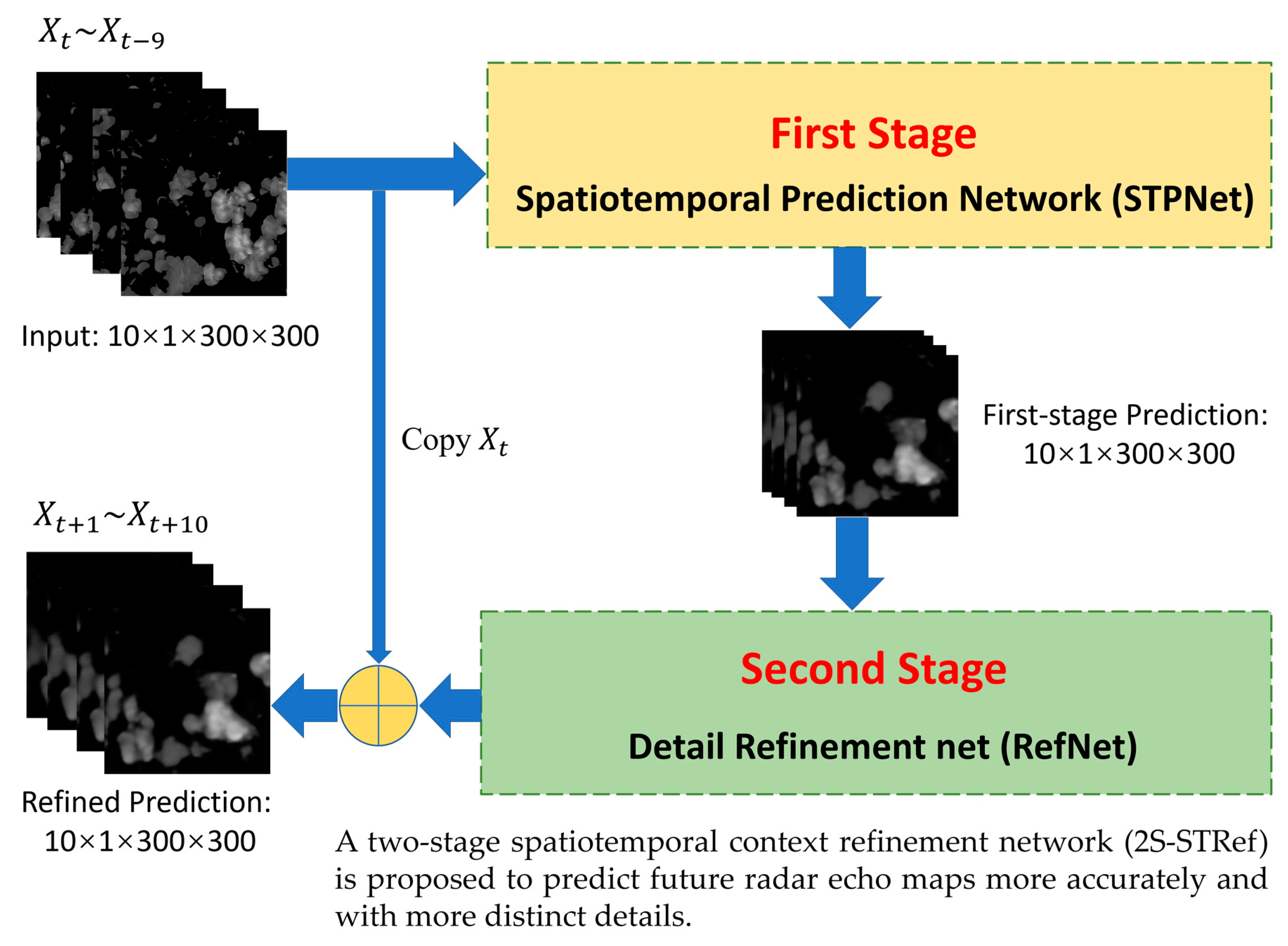
Precipitation nowcasting by radar echo extrapolation using machine learning algorithms is a field worthy of further study, since rainfall prediction is essential in work and life. Current methods of predicting the radar echo images need further improvement in prediction accuracy as well as in presenting the predicted details of the radar echo images. In this paper, we propose a two-stage spatiotemporal context refinement network (2S-STRef) to predict future pixel-level radar echo maps (deterministic output) more accurately and with more distinct details. The first stage is an efficient and concise spatiotemporal prediction network, which uses the spatiotemporal RNN module embedded in an encoder and decoder structure to give a first-stage prediction. The second stage is a proposed detail refinement net, which can preserve the high-frequency detailed feature of the radar echo images by using the multi-scale feature extraction and fusion residual block. We used a real-world radar echo map dataset of South China to evaluate the proposed 2S-STRef model. The experiments showed that compared with the PredRNN++ and ConvLSTM method, our 2S-STRef model performs better on the precipitation nowcasting, as well as at the image quality evaluating index and the forecasting indices. At a given 45 dBZ echo threshold (heavy precipitation) and with a 2 h lead time, the widely used CSI, HSS, and SSIM indices of the proposed 2S-STRef model are found equal to 0.195, 0.312, and 0.665, respectively. In this case, the proposed model outperforms the OpticalFlow method and PredRNN++ model.

1. Introduction

Nowcasting convective precipitation, which refers to the methods for near-real-time prediction of the intensity of rainfall in a particular region, has long been a significant problem in weather forecasting for its strong relation with agricultural and industrial production, as well as daily life [1,2,3]. It can issue citywide rainfall alerts to avoid casualties, provide weather guidance for regional aviation to enhance flight safety, and predict road conditions to facilitate drivers [4]. High precision and high promptness of the nowcasting precipitation leads to early prevention of major catastrophe, which means the core task of the problem is to improve the accuracy and to accelerate the prediction process [5,6]. Due to the inherent complexities of the atmosphere and relevant dynamical processes, as well as higher forecasting resolution requirement than with respect to other traditional forecasting tasks like weekly average temperature prediction, the precipitation nowcasting problem is quite challenging and has emerged as a hot research topic [7,8,9].

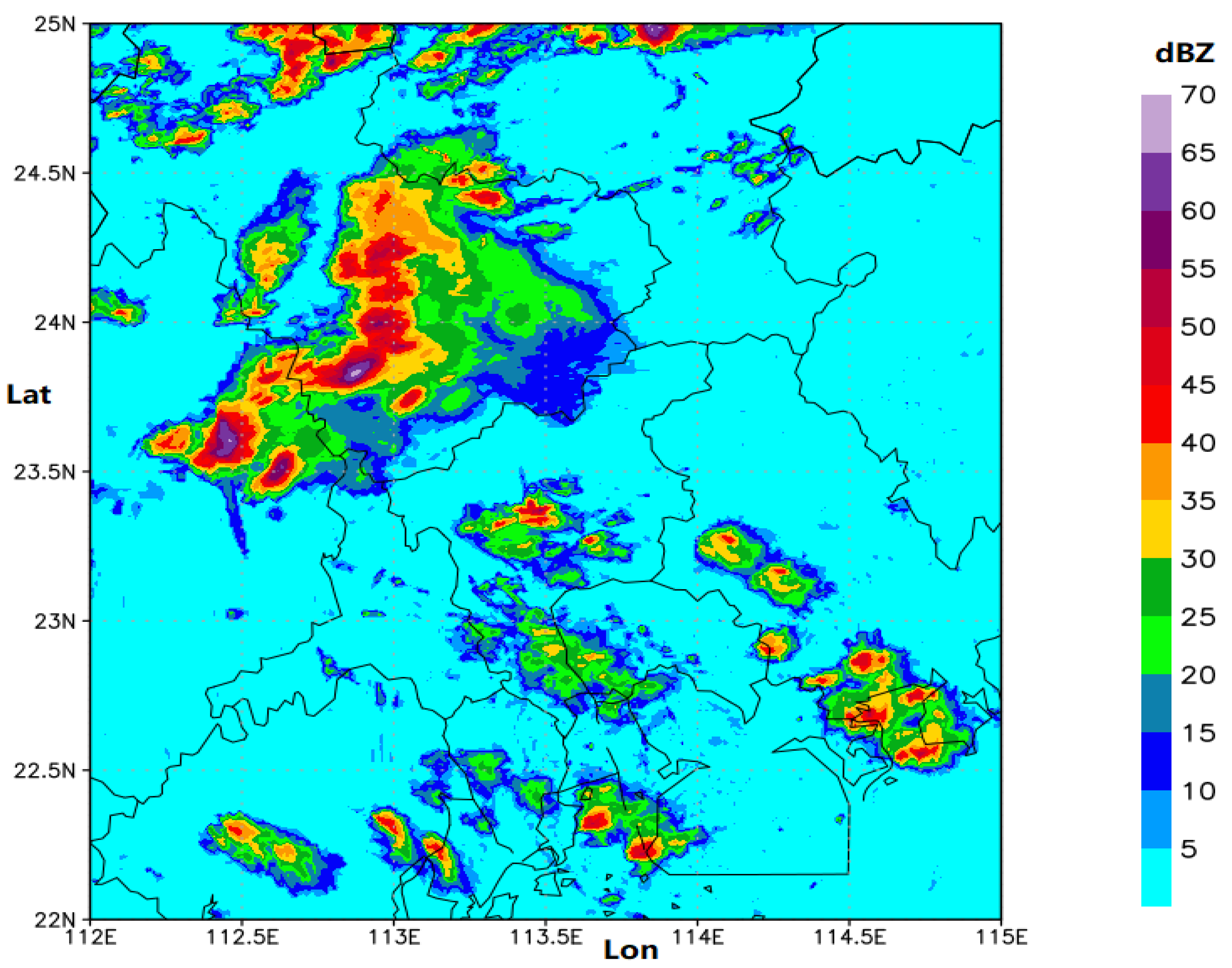
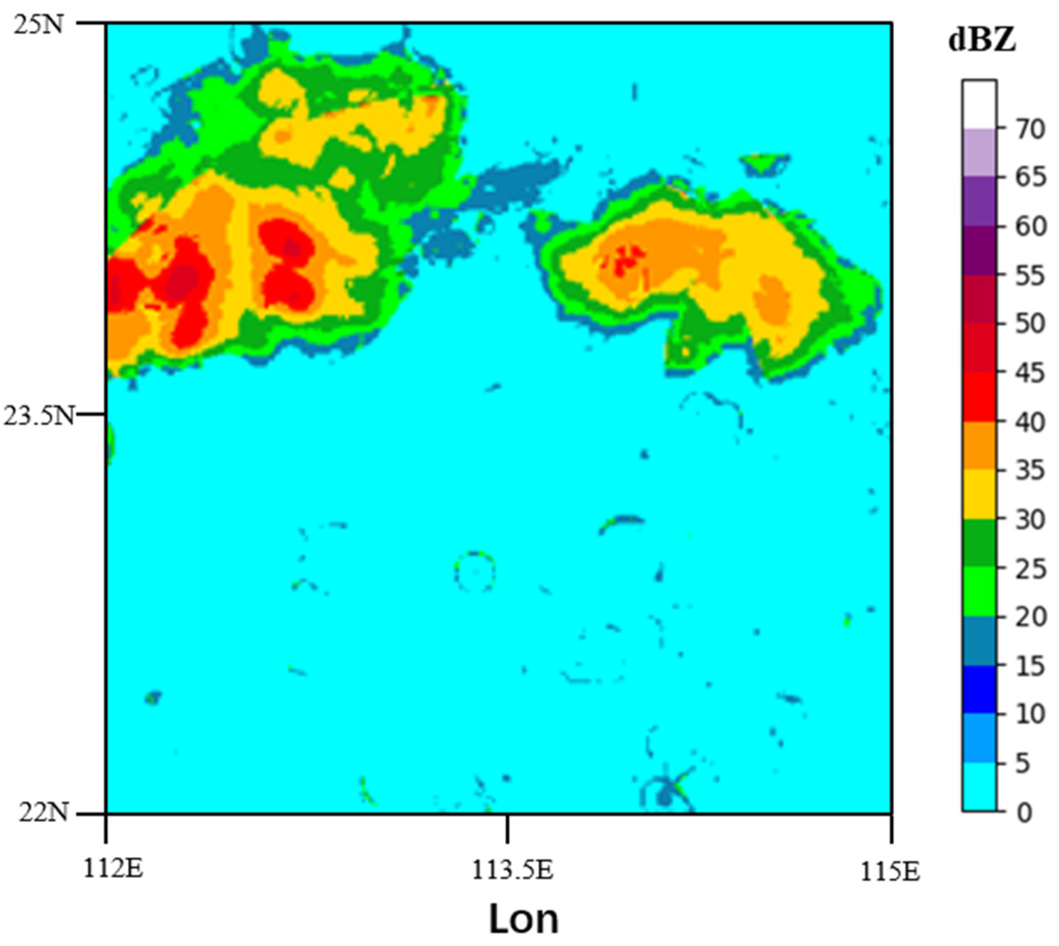
Methods to solve the problem of precipitation nowcasting can be divided into two categories [2], including methods based on the numerical weather prediction (NWP) model, and methods based on radar echo reflectivity extrapolation. Methods based on NWP calculate the prediction using massive and various meteorological data, through a complex and meticulous simulation of the physical equations in the atmosphere [10]. However, unsatisfactory prediction results are obtained if inappropriate initial states are set. For nowcasting purposes, NWP-based models are quite ineffective, especially if high-resolution and large domains are needed. Moreover, NWP-based approaches do not take full advantage of the vast amount of existing historical observation data [11,12]. Since radar echo reflectivity maps can be converted to rainfall intensity maps through the Marshall–Palmer relationship, Z(radar reflectivity)-R(precipitation intensity) relationship, and some other methods [13], nowcasting convective precipitation can be accomplished by the faster and more accurate radar echo reflectivity extrapolation [9]. The radar echo reflectivity dataset in this paper is provided by Guangdong Meteorological Bureau. An example of a radar echo reflectivity image acquired in the south China with the study area framed is shown in Figure 1. This is the radar CAPPI (Constant Altitude Plan Position Indicator) reflectivity image, which is taken from an altitude of 3 km and covers a 300 km × 300 km area centered in Guangzhou City. It is obtained from seven S-band radars, which are located at Guangzhou, Shenzhen, Shaoguan, etc. Radar echo reflectivity intensities are colored corresponding to the class thresholds defined in Figure 1.

Traditional radar echo extrapolation includes centroid tracking [13], tracking radar echoes by cross-correlation (TREC) [14], and the optical flow method [15,16,17]. The centroid tracking method is mainly suitable for the tracking and short-term prediction of heavy rainfall with strong convection. TREC is one of the most classical radar echo tracking algorithms, which calculates the correlation coefficient of radar echo in the first few moments and obtains the displacement of echo to predict the future radar echo motion. Instead of computing the maximum correlation to obtain the motion vector like TREC, the McGill Algorithm for Precipitation nowcasting using Lagrangian Extrapolation (MAPLE [18,19]) employs the variational method to minimize a cost function to define the motion field that then advects the radar echo images for nowcasting [20]. The major drawback of the extrapolation-based nowcasting is that capturing the growth and decay of the weather system and the displacement uncertainty is difficult [20]. To overcome this issue, blending techniques are applied to improve nowcasting systems, such as the Short-Term Ensemble Prediction System (STEPS [21]). In [20], a blending system is formed by synthesizing the wind information from the model forecast with the echo extrapolation motion field via a variational algorithm to improve the nowcasting system. The blending scheme performed especially well after a typhoon made landfall in Taiwan [20]. Moreover, some nowcasting rainfall models based on the advection-diffusion equation with non-stationary motion vectors are proposed in [22] to obtain smoother rainfall predictions for lead times and increase skill scores. The motion vectors are updated in each time step by solving the two-dimensional (2-D) Burgers’ equations [22]. The optical flow-based methods are proposed and widely utilized by various observatory stations [17]. The well-known Pysteps [23] supplies many optical flow-based methods, such as Extrapolation nowcast using the Lucas–Kanade tracking approach and Deterministic nowcast with S-PROG (Spectral Prognosis) [21]. In the S-PROG nowcast method, the motion field is estimated using the Lucas–Kanade optical flow and then is used to generate a deterministic nowcast with the S-PROG model, which implements a scale filtering approach in order to progressively remove the unpredictable spatial scales during the forecast [23]. The optical flow-based methods first estimate the convective precipitation cloud movements from the observed radar echo maps and then predict the future radar echo maps using semi-Lagrangian advection [9]. However, two key assumptions limit its performance: (1) the total intensity remains constant; (2) the motion contains no rapid nonlinear changes and is very smooth [24,25]. Actually, the radar echo intensity may vary over time and the motion is highly dynamic in the radar echo map extrapolation. Moreover, the radar echo extrapolation step is separated from the flow estimation step, and then the model parameters are not easy to determine to obtain good prediction performance. Furthermore, many optical flow-based methods do not only make the most of abundant historical radar echo maps in the database, but also utilize the given radar echo map sequence for prediction.

With the improvement of computing power, machine learning algorithms have boosted great interest in radar echo extrapolation [26,27,28,29], which is essentially a spatiotemporal sequence forecasting problem [30,31]. The sequences of past radar echo maps are input, and the future radar echo sequences are output. Recurrent neural network (RNN) and especially long short-term memory (LSTM) encoder-decoder frameworks in [32,33,34] are proposed to capture the sequential correlations and provide new solutions to solve the sequence-to-sequence prediction problem. Klein et al. [35] proposed a “dynamic convolutional layer” for extracting spatial features and forecasting rain and snow.

To capture the spatiotemporal dependency and predict radar echo image sequence, Shi et al. [9] developed conventional LSTM and designed convolutional LSTM (ConvLSTM), which can capture the dynamic features among the image sequence. Additionally, they further proposed the trajectory gated recurrent unit (TrajGRU) model [4], which is more flexible than ConvLSTM by the location-variant recurrent connection structure and outperforms on the grid-wise precipitation nowcasting task. Wang et al. [36] presented a predictive recurrent neural network (PredRNN) and utilized a unified memory pool to memorize both spatial appearances and temporal variations. PredRNN++ [37] further introduced a gradient unit module to capture the long-term memory dependence and achieved better performance than the previous TrajGRU and ConvLSTM methods. In addition, hybrid methods combine the effective information of observation data (radar echo data and other meteorological parameters) and numerical weather prediction (NWP) data to further enhance the prediction accuracy. A Unet-based model on the fusion of rainfall radar images and wind velocity produced by a weather forecast model is proposed in [7] and improves the prediction for high precipitation rainfalls. Moreover, the dual-input dual-encoder network structures are also proposed to extract simulation-based and observation-based features for prediction [38,39]. The limitation of the existing deep learning models lies in the defect of the extracting ability of spatiotemporal characteristics. Moreover, detailed information loss in the long-term extrapolation often occurs, which leads to blurry prediction images [40,41,42,43]. To further enhance the prediction accuracy and preserve the sharp details of predicted radar echo maps, we propose a new model, the two-stage spatiotemporal context refinement network for precipitation nowcasting (2S-STRef), in this work. The proposed model generates first-stage prediction using a spatiotemporal predictive model, then it refines the first-stage results to obtain higher accuracy and more details. We use a real-world radar echo map dataset of South China to evaluate 2S-STRef, which outperforms the traditional optical flow method and two representative deep learning models (ConvLSTM as well as and PredRNN++) in both image and forecasting evaluation metrics.

The remainder of this paper is organized as follows. Section 2 introduces the problem statement and details the proposed 2S-STRef framework, followed by descriptions of the dataset, the evaluation index, and the performance evaluation of real-world radar echo experiments in Section 3. Section 4 is a general conclusion to the whole research.

2. Methods

The short-term precipitation prediction algorithms based on radar echo images need to extrapolate a fixed length of the future radar echo maps in a local region from the previously observed radar image sequence first [44], and then obtain the short-term precipitation prediction according to the relationship between the echo reflectivity factor and rainfall intensity value. In practical applications, the radar echo maps are usually sampled from the weather radar every 6 or 12 min in China (5 min in some public datasets [23]) and forecasting is usually done for lead times from 5, 6, or 12 min to 2 h [9,23], i.e., to predict the 10 frames ahead in this work (one frame every 12 min). The reviewed methods of spatiotemporal series prediction have limited ability of extracting spatiotemporal features and the fine-level information can be lost, which leads to unsatisfactory prediction accuracy. To achieve fine-grained spatiotemporal feature learning, this paper designs a two-stage spatiotemporal context refinement network.

In general, there are three main innovation ideas:

• A new two-stage precipitation prediction framework is proposed. On the basis of the spatiotemporal sequence prediction model capturing the spatiotemporal sequence, a two-stage model is designed to refine the output.
• An efficient and concise prediction model of the spatiotemporal sequence is constructed to learn spatiotemporal context information from past radar echo maps and output the predicted sequence of radar echo maps in the first stage.
• In the second stage, a new structure of the refinement network (RefNet) is proposed. The details of the output images can be improved by multi-scale feature extraction and fusion residual block. Instead of predicting the radar echo map directly, our RefNet outputs the residual sequence for the last frame, which further improves the whole model’s ability to predict the radar echo maps and enhances the details.

In this section, the precipitation nowcasting problem will be formulated and a two-stage prediction and refinement model will be proposed.

2.1. Formulation of Prediction Problem

Weather radar is one of the best instruments to monitor the precipitation system. The intensity of radar echo is related to the size, shape, state of precipitation particles, and the number of particles per unit volume. Generally, the stronger the reflected signal is, the stronger the precipitation intensity is. Therefore, the intensity and distribution of precipitation in a weather system can be judged by the radar echo map.

The rainfall rate values (mm/h) can be calculated by the radar reflectivity values using the Z–R relationship. Z is the radar reflectivity values and R is the rain-rate level.

It means that if we can predict the following radar echo images by inputting the previous frames, we can achieve the goal of precipitation nowcasting.

In this work, the 2-D radar echo image at every timestamp is divided into tiled non-overlapping patches, whose pixels are measurements. The short-term and temporary precipitation nowcasting naturally becomes capturing the spatiotemporal features and extrapolating the sequences of future radar echo images. The observation image can be represented as a tensor $X_t\in R^{C\times W\times H}$, representing the image at time t, where R denotes the observed feature domain, $C$ refers to the channel number of feature maps, and $W$ and $H$ represent the width and height of the state and input tensors, respectively. ${\widehat{X}}_t$ is used to represent the predicted radar echo image at time t. Therefore, the problem can be described as (1):

$${\widehat{X}}_{t+1} \dots ,{\widehat{X}}_{t+K}=\underset{X_{t+1},\dots ,X_{t+K}}{\mathrm{argmax}}p(X_{t+1},\dots ,X_{t+K}|{\tilde{X}}_{t-J+1},{\tilde{X}}_{t-J+2},\dots ,{\tilde{X}}_t),$$

(1)

The main task is to predict the most likely length-K radar echo maps ${\widehat{X}}_{t+1} \dots ,{\widehat{X}}_{t+K}$ based on the previous J observations including the current one (${\tilde{X}}_{t-J+1},{\tilde{X}}_{t-J+2},\dots ,{\tilde{X}}_t$) and make them as close as possible to the real observations $X_{t+1},\dots ,X_{t+K}$ for the next time slots. In this paper, 10 frames are put into the network and the next 10 frames are expected to be output, i.e., $K=10, J=10$ in (1).

2.2. Network Structure

Figure 2 illustrates the overall architecture of 2S-STRef. The network framework is composed of two stages.

The first stage, named the spatiotemporal prediction network (STPNet), is an encoder-decoder structure based on the spatiotemporal recurrent neural network (ST-RNN), which is inspired by ConvLSTM [9] and TrajGRU [4] and has convolutional structures in both the input-to-state and state-to-state transitions. We input the previous radar echo observation sequence into the encoder of STPNet and obtain n layers of RNN states, then utilize another n layers of RNNs to generate the future radar echo predictions based on the encoded status. The prediction is the first-stage result and is an intermediate result.

The second stage, named the detail refinement stage, proposed in this paper acts as a defuzzification network for the predicted radar echo images, and also improves the ability of spatial and temporal feature extraction for echo image detail information. We input the first-stage prediction into the detail refinement stage to acquire a refined prediction, which is also the final result with improvement of the radar echo image quality and promotion of precipitation prediction precision.

Two stages will be introduced in detail in the following subsections.

2.2.1. First Stage: Spatiotemporal Prediction Net

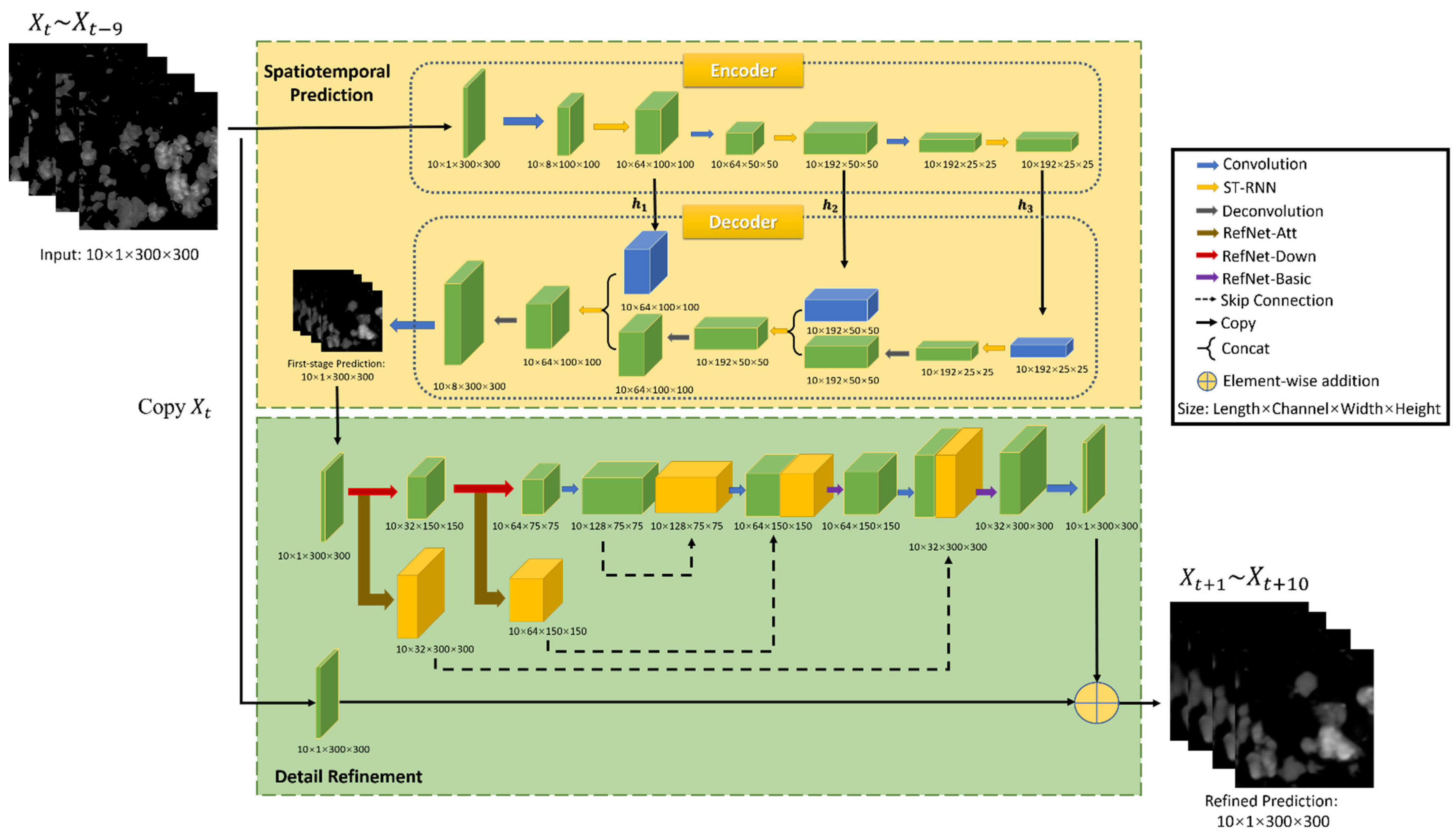
Inspired by the models [4,9,35], an end-to-end spatiotemporal prediction network (STPNet) based on the encoder-decoder network frame is designed to compensate the translation invariance of convolution when capturing spatiotemporal correlations. For moving and scaling in the precipitation area, the local correlation structure should be changed with different timestamp and spatial locations. STPNet can effectively represent such a location–variant connection relationship, whose structure is shown in the dotted box with a yellow background of Figure 2.

ST-RNN. The precipitation process based on radar echo maps will naturally have random rotation and elimination. In ConvLSTM, location-invariant filters are used by the convolution operation to the input, which is thus inefficient. We designed ST-RNN, which employs the current input and the state of the previous step to obtain a local neighborhood set of each location at each timestamp. A set of continuous flows is used to represent the discrete and non-differentiable location indices. The specific formula of ST-RNN is given in Equation (2):

$$\begin{array}{cc}\hfill {\mathcal{U}}_t,{\mathcal{V}}_t=& \gamma ({\mathcal{X}}_t,{\mathscr{H}}_{t-1})\hfill \\ \hfill i_t=& \sigma ({\mathcal{W}}_{xi}\ast {\mathcal{X}}_t+{\sum }_{l=1}^L{W}_{hi}^l\ast g({\mathscr{H}}_{t-1},{\mathcal{U}}_{t,l},{\mathcal{V}}_{t,l}))\hfill \\ \hfill f_t=& \sigma ({\mathcal{W}}_{xf}\ast {\mathcal{X}}_t+{\sum }_{l=1}^L{W}_{hf}^l\ast g({\mathscr{H}}_{t-1},{\mathcal{U}}_{t,l},{\mathcal{V}}_{t,l}))\hfill \\ \hfill {\tilde{\mathcal{C}}}_t=& \tan \mathrm{h}({\mathcal{W}}_{xc}\ast {\mathcal{X}}_t+{\sum }_{l=1}^L{W}_{hc}^l\ast g({\mathscr{H}}_{t-1},{\mathcal{U}}_{t,l},{\mathcal{V}}_{t,l}))\hfill \\ \hfill {\mathcal{C}}_t=& f_t\circ {\mathcal{C}}_{t-1}+i_t\circ {\tilde{\mathcal{C}}}_t\hfill \\ \hfill o_t=& \sigma ({\mathcal{W}}_{xo}\ast {\mathcal{X}}_t+{\sum }_{l=1}^L{W}_{ho}^l\ast g({\mathscr{H}}_{t-1},{\mathcal{U}}_{t,l},{\mathcal{V}}_{t,l}))\hfill \\ \hfill {\mathscr{H}}_t=& o_t\circ \tan \mathrm{h}({\mathcal{C}}_t)\hfill \end{array}$$

(2)

In the formula, ‘*’ is the convolution operation and ‘∘’ is the Hadamard product. $\sigma$ is the sigmoid activation function. L is the number of links and ${\mathcal{U}}_t,{\mathcal{V}}_t\in {ℝ}^{L\times H\times W}$ are the flow fields storing local connections, whose generating network is $\gamma$. ${\mathcal{W}}_{hi}^l, {\mathcal{W}}_{hf}^l , {\mathcal{W}}_{hc}^l,{\mathcal{W}}_{ho}^l$ refers to the weights for projecting the channels. Function $g(ℐ, U,V)$ is used to generate location information from ${\mathcal{U}}_t,{\mathcal{V}}_t$ by double linear sampling [4]. We represent $ℳ=g(ℐ, U,V)$, where $ℳ,ℐ\in {ℝ}^{C\times H\times W}$ and $U,V\in {ℝ}^{H\times W}$, which can be stated as Equation (3):

$$\begin{array}{c}\hfill {ℳ}_{c,i,j}={\displaystyle \sum _{m=1}^H}{\displaystyle \sum _{n=1}^W}{ℐ}_{c,m,n}\times max(0,1-|i+V_{i,j}-m|)\\ \hfill \times max(0,1-|j+U_{i,j}-n|)\end{array}$$

(3)

The connection topology can be obtained from the parameters of the subnetwork $\gamma$, whose input is the concatenation of ${\mathcal{X}}_t \mathrm{and} {\mathscr{H}}_{t-1}$. The subnetwork $\gamma$ adopts a simple convolutional neural network and nearly no additional computation cost is added.

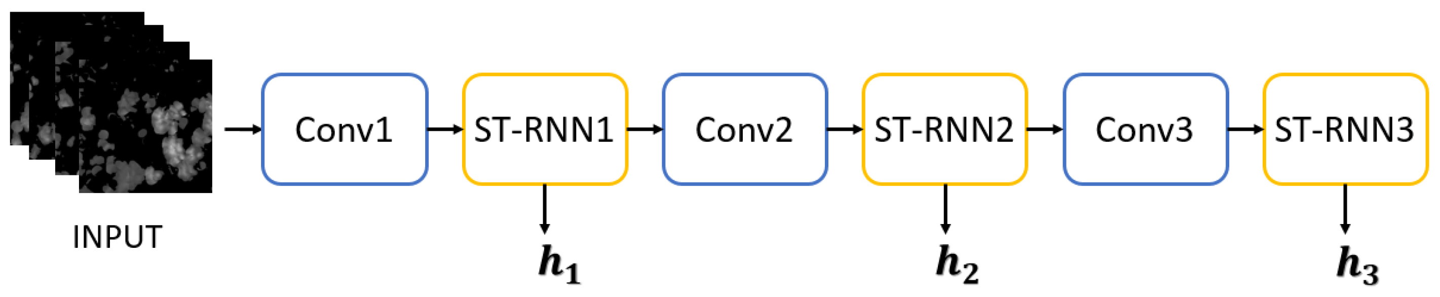
For our spatiotemporal sequence forecasting problem, ST-RNN net is the key building block used in the whole encoder-decoder network structure. This structure is similar to the predictor model in [4,9]. The encoder network (shown in Figure 3) is in charge of compressing the recent radar echo observation sequence ${[{\tilde{X}}_t]}_{t=t-J+1}^t$ into $n$ layers of ST-RNNs and the decoder network (shown in Figure 4) unfolds these encoder states to generate the most likely length-$K$ predictions ${[{\widehat{X}}_t]}_{t=t+1}^{t+K}$. Three-dimensional tensors are employed in the input and output elements to preserve the spatial information.

$$\begin{array}{c}{\widehat{X}}_{t+1} \dots ,{\widehat{X}}_{t+K}=\underset{X_{t+1},\dots ,X_{t+K}}{\mathrm{argmax}}p(X_{t+1},\dots ,X_{t+K}|{\tilde{X}}_{t-J+1},{\tilde{X}}_{t-J+2},\dots ,{\tilde{X}}_t)\\ \approx g_{decoder}(f_{encoder}({\tilde{X}}_{t-J+1},{\tilde{X}}_{t-J+2},\dots ,{\tilde{X}}_t))\end{array}$$

(4)

Encoder. The structure of the encoder, shown in Figure 3, is formed by stacking Convolution, ST-RNN, Down Sampling, ST-RNN, Down Sampling, and ST-RNN. The input sequence of radar echo images first passes through the first convolution layer to extract the spatial feature information of each echo image. The resolution is reduced, and the output feature image size is 100 × 100. Then, the local spatiotemporal feature information of the echo images is extracted at a low scale through the ST-RNN layer, and the hidden state $h_1$ is output. At the same time, the output feature map is sent to the lower sampling layer to extract the spatial features of high-level spatial scale, whose size is now 50 × 50. The second ST-RNN layer is used to extract the spatial and temporal features of mesoscale and output the hidden state $h_2$. The output result of the second layer ST-RNN is transferred to the second lower sampling layer whose size is 25 × 25. The last convolution layer extracts the spatial features of higher spatial scale, and outputs the feature map to the last ST-RNN layer, which outputs the hidden state $h_3$. In this paper, three stacked ST-RNN layers are used [4]. Few ST-RNN layers do not have strong enough representational power for spatiotemporal features and prediction accuracy will be affected. A large number of ST-RNN layers will increase the difficulty of training and the network is easy to overfit.

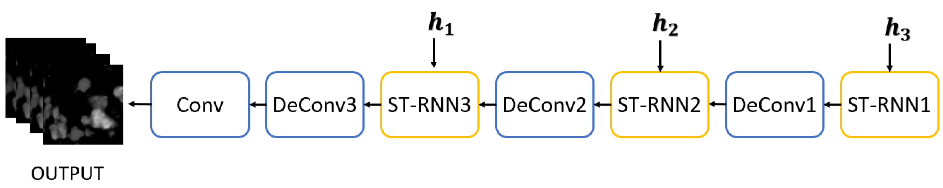
Decoder. The structure of the decoder, shown in Figure 4, is dual to that of the encoder, including ST-RNN, Up Sampling, ST-RNN, Up Sampling, ST-RNN, Deconvolution, and Convolution. The order of the decoder network is reversed, where the high-level states capturing the global spatiotemporal representation are utilized to influence the update of the low-level states. When the decoder is initialized, all ST-RNN layers receive the hidden states $h_1$, $h_2$, and $h_3$ from the encoder, respectively. Firstly, the encoder sends $h_3$ to the top-level ST-RNN, and transmits the output results to the upper sampling layer to fill in details at high scale. The output feature map size is now 50 × 50. Then, through the middle ST-RNN layer, the prediction is carried out on the mesoscale with the received hidden state $h_2$. The predicted output feature map is sent to the second upsampling layer to fill in the details on the mesoscale, and the size of the output feature map is 100 × 100. The lowest level ST-RNN layer receives the hidden state $h_1$ and the mesoscale feature map, and makes prediction on the small scale. Finally, through the deconvolution layer, by combining features and filling in the small-scale image details, the first-stage radar echo prediction image sequence is output.

Table 1. General structure of the encoder of the proposed spatiotemporal RNN model (stage 1).

Name	Kernel	Stride	L	Channels Input/Output
Conv1	5 × 5	3 × 3	−	1/8
ST-RNN1	3 × 3	1 × 1	13	8/64
Conv2	3 × 3	2 × 2	−	64/64
ST-RNN2	3 × 3	1 × 1	13	64/192
Conv3	3 × 3	2 × 2	−	192/192
ST-RNN3	3 × 3	1 × 1	9	192/192

and

Table 2. General structure of the decoder of the proposed spatiotemporal RNN model (stage 1).

Name	Kernel	Stride	L	Channels Input/Output
ST-RNN1	3 × 3	1 × 1	9	192/192
DeConv1	4 × 4	2 × 2	−	192/192
ST-RNN2	3 × 3	1 × 1	13	192/192
DeConv2	4 × 4	2 × 2	−	192/192
ST-RNN3	3 × 3	1 × 1	13	192/64
DeConv3	5 × 5	3 × 3	−	64/8

show the detailed structure settings of the encoder and decoder of our spatiotemporal RNN model. Kernel is a matrix that moves over the input data, and performs the dot product with the sub-region of input data. Stride defines the step size of the kernel when sliding through the image. L is the number of links in the state-to-state transition.

2.2.2. Second Stage: Detail Refinement Net

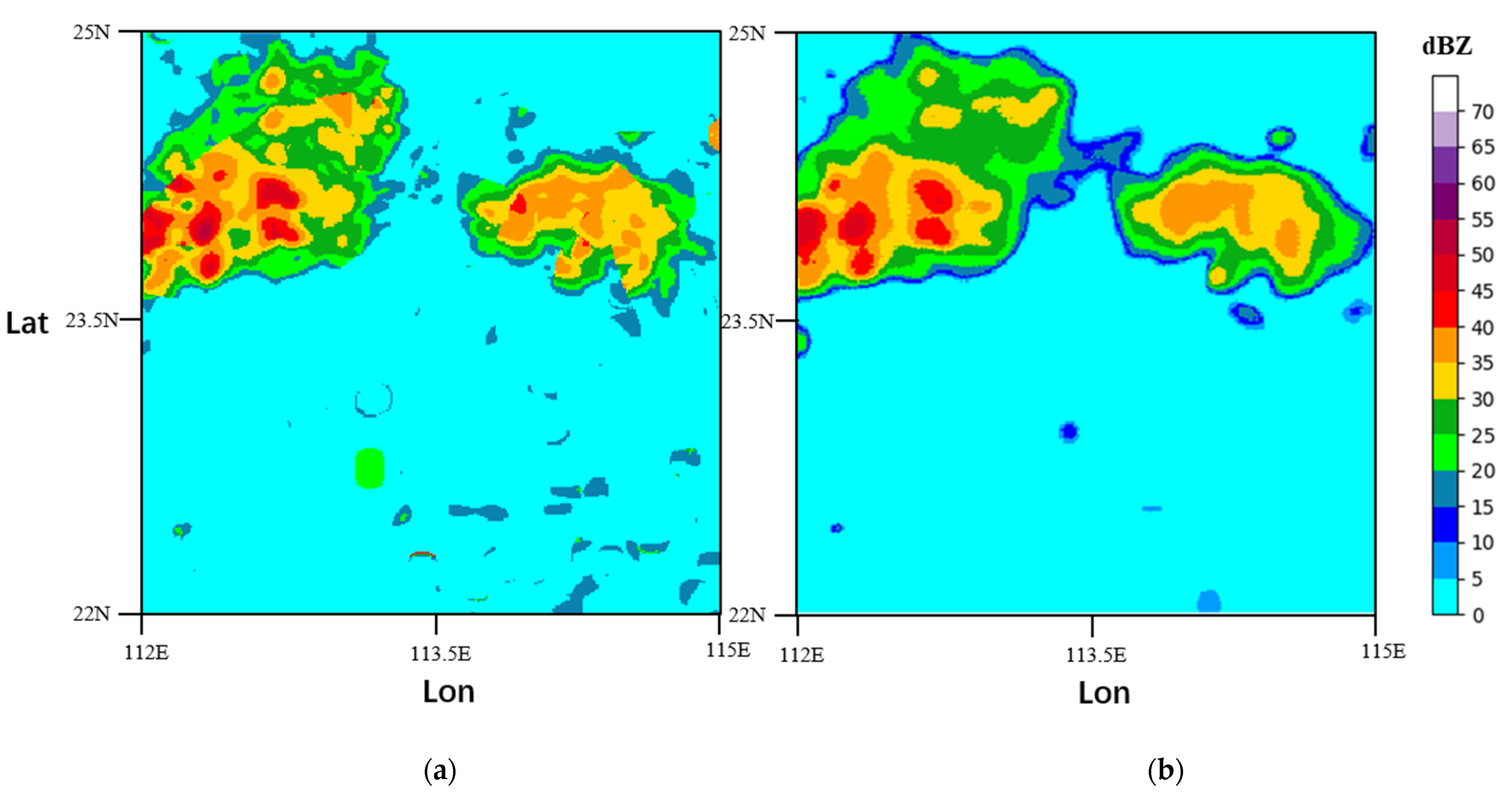
Although the predicted images by the first-stage STPNet already perform well and have high prediction accuracy, the extrapolation radar echo images still seem to be blurred and lack details [9,45,46], as shown in Figure 5b. Therefore, the second-stage network (RefNet) is proposed to further extract spatiotemporal features and refine the predicted radar echo sequences.

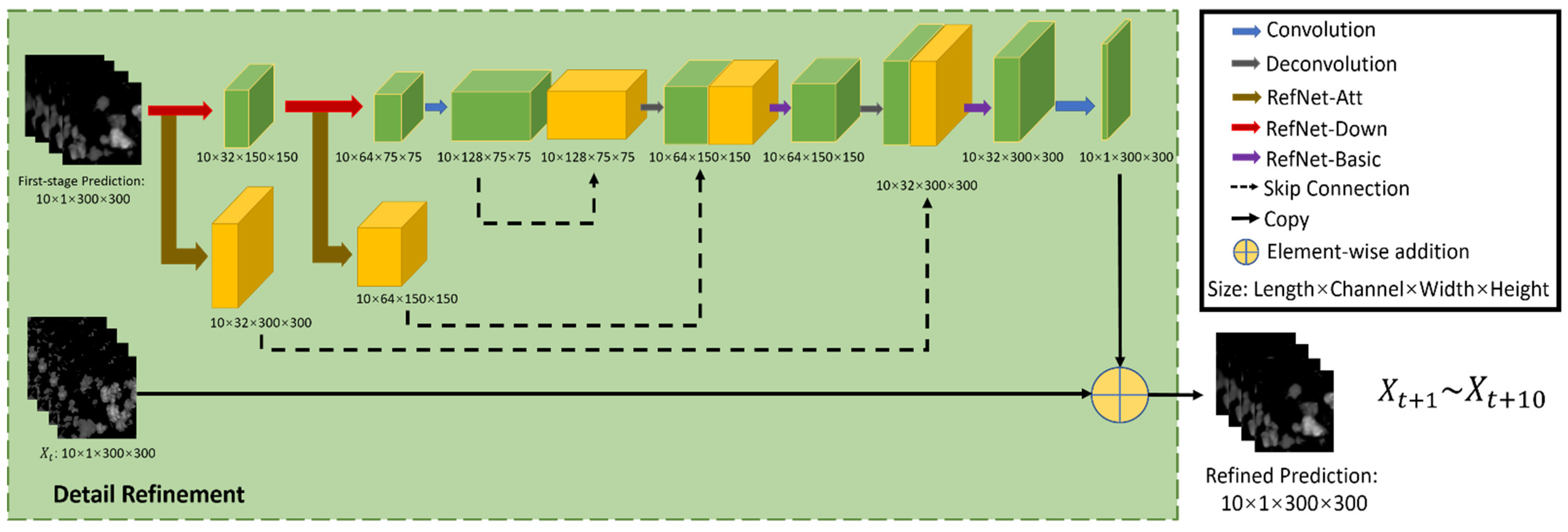
The overall architecture of the proposed RefNet is shown in Figure 6. The details of the predicted radar echo images can be improved by multi-scale feature extraction and fusion residual block. An encoder–decoder network is utilized to implement high-frequency enhancement, which serves as a feature selector for focusing on the locations full of tiny textures. Meanwhile, multi-level skip connection is employed between different-scale features for feature sharing and reuse. Both local and global residual learning is integrated for preserving the low-level features and decreasing the difficulty of training and learning. Different hierarchical features are combined to generate finer features, which favor the reconstruction of high-resolution images. The widely used stride r = 2 is chosen in the downsampling layers and upsampling layers. Finally, a 1 ×1 convolution layer at the end of the RefNet outputs the residual sequence for the last frame. This operation could further improve the whole model’s ability to predict the radar echo map sequence and enhance the details.

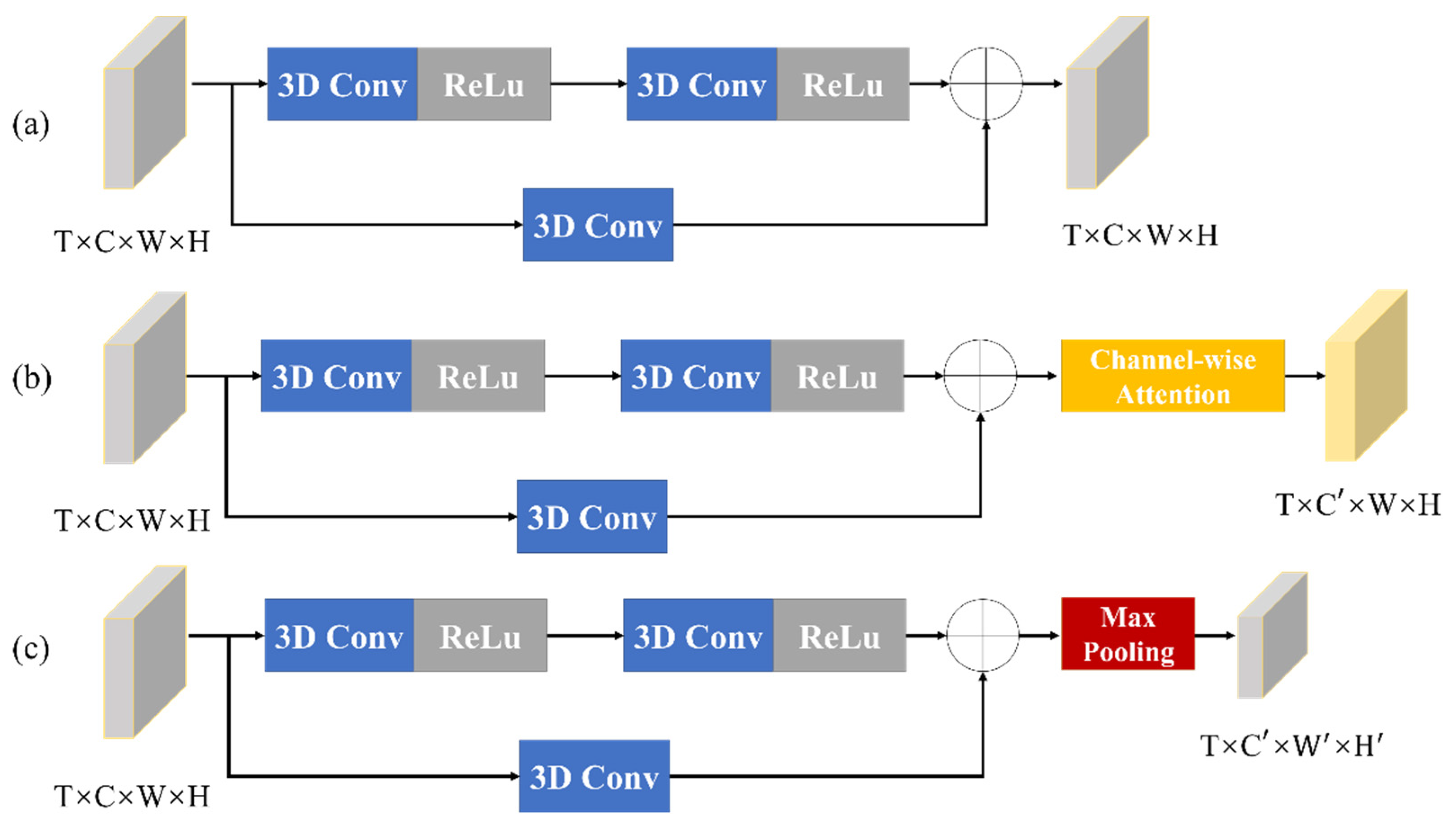
Three subnets are defined to build up the RefNet, named RefNet-Basic (purple arrow in Figure 6), RefNet-Att (brown arrow in Figure 6), and RefNet-Down (red arrow in Figure 6). The blue arrow denotes the convolution operation. Among those modules, RefNet-Basic, shown in Figure 7a, is the basic module of the other two modules. The RefNet-Basic module is composed of 3-D conv layers with different depths. It generates and combines different hierarchical features that are useful for low-level feature learning [47]. The low-level feature means edge, texture, and contours in images. The high-level feature means sematic information. Different hierarchical high-level features are fused to help the reconstruction of low-level features. Residual connections are employed for both local and global feature extraction, which make the multi-scale feature information flow more efficiently in the network and mitigate the difficulty of network training.

Intuitively, the high-resolution feature maps have more high-frequency details than those of low-resolution feature maps [48,49]. In each RefNet-Basic module, multiple local features are extracted in the encode process, and then reused in the decode process. The fusion operation will merge multi-level feature maps from different phases into decoded feature maps. The operation $\oplus$ in Figure 6 and Figure 7 is performed using a shortcut connection and element-wise addition.

As shown in Figure 7b, RefNet-Att is a RefNet-Basic module followed by channel-wise attention operation to preserve the discriminative features and details to the most extent. In this work, the SE (squeeze-and-excitation) operation [50] is incorporated as an attention mechanism for learning the spatio-temporal feature importance, and producing the importance weight matrix for input feature map sequences. In Figure 7c, the RefNet-Down is a RefNet-Basic module followed by the max-pooling operation, which is used to compress the input feature map. The input feature maps are progressively downsampled into small-scale abstractions through successive RefNet-Down modules. Specifically, the RefNet-Down with stride r = 2 is utilized as the downsampling layer. In the expansive part, the deconvolution layers are then used to upsample the obtained abstractions back to the previous resolution. Therefore, the deconvolution layer with stride r = 2 is utilized to upsample the upper features.

Figure 8 presents an example of predicted radar echo images with just the first-stage STPNet method and the whole 2S-STRef method. From Figure 5b and Figure 8, it is clear that the proposed 2S-STRef method integrating the second-stage RefNet is able to produce sharper predicted radar echo images with more details compared with only the first-stage STPNet method.

2.3. Loss Function

In addition, the frequencies of different intensities of rainfall are outstandingly imbalanced, so weighted loss is utilized to alleviate this problem. As defined in Equation (5), we designed different weights for different radar echo reflectivity Z (denoting different rainfall intensities):

$$w(z)=\{\begin{array}{cc}1,\hfill & Z<20 \mathrm{dBZ}\hfill \\ 2,\hfill & 20 \mathrm{dBZ}\le Z<35 \mathrm{dBZ}\hfill \\ 6,\hfill & 35 \mathrm{dBZ}\le Z<45 \mathrm{dBZ}\hfill \\ 60, \hfill & Z\ge 45 \mathrm{dBZ}\hfill \end{array},$$

(5)

The weighted loss function we designed is shown in Equation (6):

$$\begin{array}{c}ℒ=\frac{1}{N}{\sum }_{n=1}^N{\sum }_{i,j}(w_{n,i,j}({({\tilde{y}}_{n,i,j}-y_{n,i,j})}^2+|{\tilde{y}}_{n,i,j}-y_{n,i,j}|)\\ +1-\mathrm{SSIM}({\tilde{y}}_{n,i,j},y_{n,i,j}))\end{array}$$

(6)

where N represents the number of all images in the predicted sequence, and $w_{n,i,j}$ represents the weight of the (i, j)th pixel at the n-th frame. $y_{n,i,j}$ and ${\tilde{y}}_{n,i,j}$ are the values of (i, j)th of the n-th ground-truth radar echo image and the n-th predicted image, respectively. $\frac{1}{N}{\sum }_{n=1}^N{\sum }_{i,j}{w}_{n,i,j}{({\tilde{y}}_{n,i,j}-y_{n,i,j})}^2$ can be denoted as B(Balanced)-MSE and $\frac{1}{N}{\sum }_{n=1}^N{\sum }_{i,j}{w}_{n,i,j}|{\tilde{y}}_{n,i,j}-y_{n,i,j}|$ as B-MAE. More weights are assigned to bigger radar echo reflectivity in the calculation of MSE and MAE to enhance the prediction performance for heavy precipitation. In this way, a lack of samples with heavy rain can be compensated. Our main goal is to learn a network to ensure that the predicted radar echo image ${\tilde{y}}_{n,i,j}$ is as close as possible to the ground truth image $y_{n,i,j}$. The SSIM (structural similarity) loss is combined with the loss function, which can further enhance the details of the output images [51].

2.4. Implementation

All models are optimized using the Adam optimizer with a learning rate equal to 10−4. These models are trained with early stopping on the sum of SSIM, B-MSE, and B-MAE. In the ROVER, the mean of the last two flow fields is employed to initialize the motion field [9]. The training batch size in the RNN models is set to 4. For the STPNet and ConvLSTM models, a 3-layer encoding-forecasting structure is used and the numbers of filters for the RNNs are set to 64, 192, and 192. The kernel sizes (5 × 5, 5 × 5, 3 × 3) are used in the ConvLSTM models. For the STPNet model, the numbers of links are set as 13, 13, and 9.

The implementation details of the proposed RefNet are shown in

Table 3. Implementation details of the proposed method.

Hyper-Parameter	Value
numbers of hidden states	64, 128, 256
kernel sizes	3 × 3
Rotation angle	30°
Optimizer	Adam (β1 = 0.9, β2 = 0.999)
Minibatch size	4
Learning rate	1 × 10−4
Framework	Pytorch 1.7
GPU	NVIDIA RTX 3090

. A 3-layer encoding-forecasting structure is utilized and the numbers of hidden states (64, 128, 256) are set. The kernel sizes of all convolutional layers except that in the output operations (the kernel size is 1 × 1) are set as 3 × 3. Zero padding around the boundaries of radar echo images is performed before convolution to keep the size of the feature maps unchanged. All training data are randomly rotated by 30° and flipped horizontally. The model is trained with the Adam optimizer [52] by setting β1 = 0.9, β2 = 0.999. The minibatch size is 4. The learning rate is initialized as 1 × 10⁻⁴ and decreased by 0.7 at every 10 epoch.

We implemented the proposed method with the Pytorch 1.7 framework and trained it using NVIDIA RTX 3090 GPU and Cuda 11.0. The default weight initialization method in Pytorch 1.7 was used.

3. Experiments

3.1. Radar Echo Image Dataset

Introduction to dataset. As shown in Equation (1), rainfall intensity can be inferred by radar reflectivity values. Precipitation nowcasting accomplished by deep learning methods needs a large number of radar echo images. In this paper, the radar echo dataset is a subset of the three-year weather radar echo images provided by Guangdong Meteorological Bureau from 2017 to 2019. The spatial resolution is 1 km and the observation area is Southern China. In order to reduce the cost of image storage, the region covering 300 km × 300 km of the Pearl River Delta is selected, covering longitude ranges from 112° to 115° E and latitude from 22° to 25° N. The observation interval of weather radar is 12 min and there are 120 frames per day. The size of each image is 300 × 300, with each pixel representing the echo intensity within one square kilometer. Figure 1 is an example of the radar echo image.

Pre-process of the radar echo data. In general, most of the radar echo intensity lower than 10 dBZ is due to clutter caused by ground dust [53], which is noise for precipitation nowcasting, so that all pixel grid points lower than 10 dBZ in the image are set to 0. Moreover, to alleviate the noise impact in training and evaluation, the pixel values of some noisy regions are further removed by applying K-means clustering to the monthly pixel average [9]. Then, the original radar reflectivity factor will be linearly converted into the range of pixel value (0~255) in the image domain using Equation (7):

$$\mathrm{pixel} =\lfloor 255\times \frac{\mathrm{dBZ}}{70}+0.5\rfloor ,$$

(7)

Since rainfall events occur sparsely, a lack of precipitation events is actually not conducive to the network learning the spatial and temporal information of precipitation. For the validity of the dataset, those days on which there is rain are removed. The radar echo data in precipitation daily events including discontinuous rainfall in the Pearl River Delta from 2017 to 2019 are selected to form our dataset, including 356 precipitation events and 42,720 radar echo images. The details are shown in

Table 4. Details of the dataset.

Year	Images	Daily Event
2017	17,400	145
2018	13,080	109
2019	12,240	102

. Among them, the 2017 and 2018 datasets are used as the training set and verification set, with a ratio of 8:2. The 2019 dataset is used as the test set. Each daily radar echo sequence is partitioned into non-overlapping frame blocks, from which the data instances are sliced by a 20-frame-wide sliding window.

3.2. Evaluation

Image quality evaluation index. To verify the better performance of our network on rendering image details, SSIM [51] is used for evaluating the results. It is used to measure the similarity between two images, focusing on brightness, contrast, and structure [51]. It is an image quality evaluation standard in line with human intuition. The formulation is given below in Equation (8):

$$\mathrm{SSIM}(x,y)=\frac{(2{\mu }_x{\mu }_y+C_1)(2{\sigma }_{xy}+C_2)}{({\mu }_x^2+{\mu }_y^2+C_1)({\sigma }_x^2+{\sigma }_y^2+C_2)},$$

(8)

In Equation (8), $x,y$ represent the predicted radar echo image and the real image, respectively. $\mu$ represents the mean value of the image; $\sigma$ is the standard deviation of the image. ${\sigma }_{xy}$ is the covariance of $x$ and $y$, and $C_1$ and $C_2$ are constants in order to avoid the calculation error caused by division by zero. The larger the value calculated by SSIM, the more the two images are similar.

Forecasting evaluation index. The following four commonly used precipitation nowcasting metrics are used to evaluate the accuracy of the prediction, including the Critical Success Index (CSI), Heidke Skill Score (HSS), Probability of Detection (POD), and False Alarm Rate (FAR). Since our predictions are done at the pixel level, we project them back to radar echo intensities and calculate the rainfall at every cell of the grid [9]. These four evaluation indexes are similar to the classification indexes, and their main focus is whether the predicted location point hits within a certain threshold range. For example, if the threshold is 20 dBz, then 19 dBz will be converted to 0 and 21 dBz will be converted to 1 after binarization. After converting every pixel value in prediction and ground-truth to 0/1, we calculate the TP (true positive, prediction = 1, truth = 1), FN (false negative, prediction = 0, truth = 1), FP (false positive, prediction = 1, truth = 0), and TN (true negative, prediction = 0, truth = 0). Then, these four indicators can be calculated by using Equation (9). In this work, in order to obtain a full appreciation of the algorithm’s performance, the skill scores at three thresholds that correspond to different rainfall levels are calculated [54]. We choose 20 dBZ (0.5 mm/h), 35 dBZ (5 mm/h), and 45 dBZ (30 mm/h) as the thresholds to evaluate the prediction performance:

$$\begin{array}{cc}\hfill \mathrm{CSI}=& \frac{\mathrm{TP}}{\mathrm{TP}+\mathrm{FP}+\mathrm{FN}}\hfill \\ \hfill \mathrm{HSS}=& \frac{2\times (\mathrm{TP}\times \mathrm{TN}-\mathrm{FP}\times \mathrm{FN})}{(\mathrm{TP}+\mathrm{FN})(\mathrm{FN}+\mathrm{TN})+(\mathrm{TP}+\mathrm{FP})(\mathrm{FP}+\mathrm{FN})}\hfill \\ \hfill \mathrm{POD}=& \frac{\mathrm{TP}}{\mathrm{TP}+\mathrm{FN}}\hfill \\ \hfill \mathrm{FAR}=& \frac{\mathrm{FP}}{\mathrm{TP}+\mathrm{FP}}\hfill \end{array},$$

(9)

For the larger CSI, HSS, and POD that are closer to 1, the higher nowcasting accuracy of the algorithm is obtained. This is just contrary to FAR.

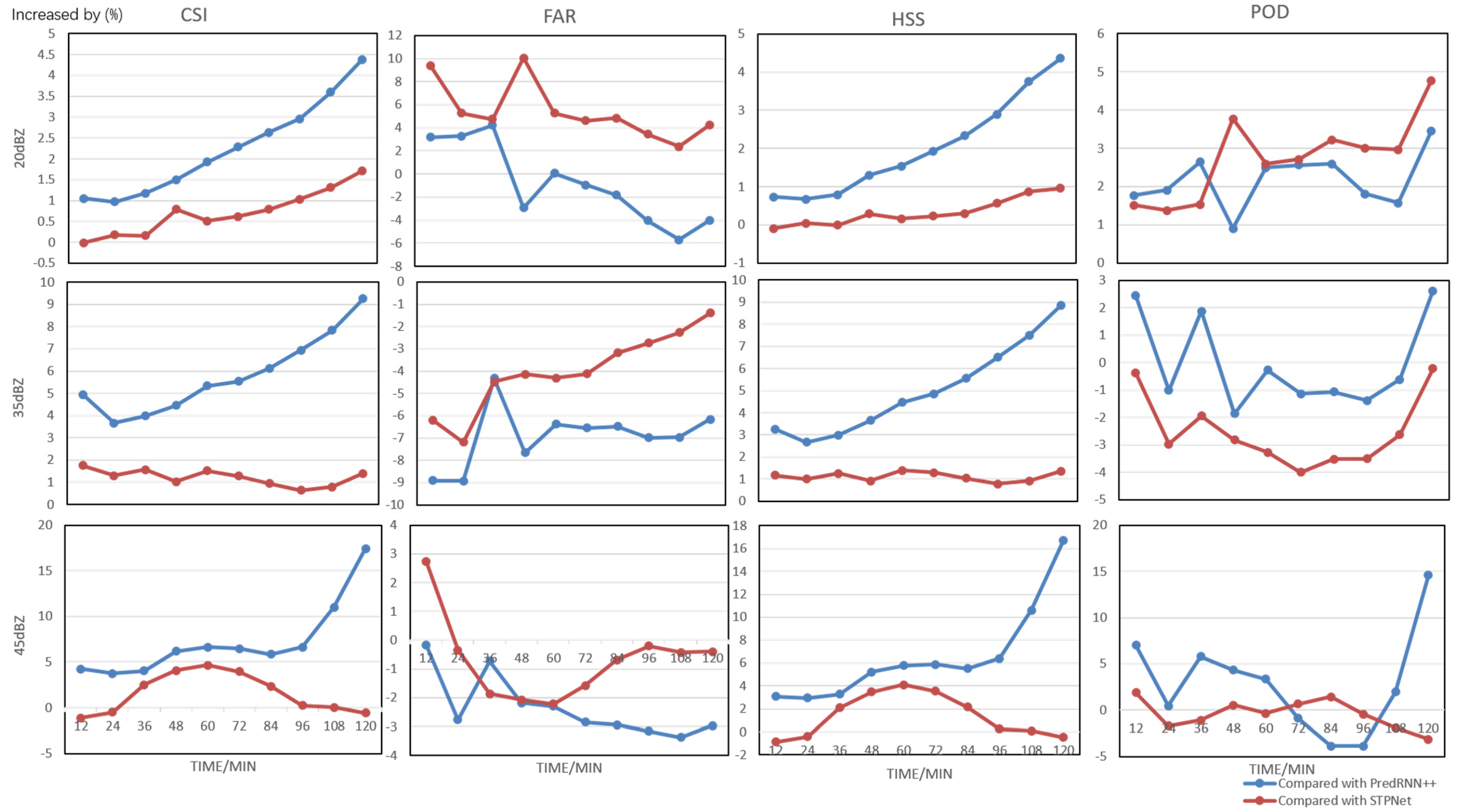
In order to depict the performance comparisons more clearly between the PredRNN++, STPnet method, and the proposed 2S-STRef method, an increasing rate is defined in Equation (10):

$$\begin{array}{cc}\mathrm{Increasing}\mathrm{rate}(\mathrm{PredRNN}++)& =\frac{\mathrm{Metric}\mathrm{scores}(2\mathrm{S}-\mathrm{STRef})-\mathrm{Metric}\mathrm{scores}(\mathrm{PredRNN}++)}{\mathrm{Metric}\mathrm{scores}(\mathrm{PredRNN}++)}\times 100\%\\ \mathrm{Increasing}\mathrm{rate}(\mathrm{STPnet})& =\frac{\mathrm{Metric}\mathrm{scores}(2\mathrm{S}-\mathrm{STRef})-\mathrm{Metric}\mathrm{scores}(\mathrm{STPnet})}{\mathrm{Metric}\mathrm{scores}(\mathrm{STPnet})}\times 100\%\end{array}$$

(10)

3.3. Results

In this section, we compare our two-stage spatiotemporal context refinement network (2S-STRef) with three typical optical flow-based methods (ROVER [17] and Pysteps [23]), and three deep learning methods (ConvLSTM [9], PredRNN++ [37], and STPNet (the first stage of our model)) on the image quality evaluation index SSIM, and on the forecasting evaluation indexes CSI, HSS, POD, and FAR.

ROVER (Real-time Optical flow by Variational methods for Echoes of Radar) [17] proposed by the Hong Kong Observatory (HKO) calculates the optical flow of consecutive radar maps and performs semi-Lagrangian advection on the flow field to accomplish the prediction [9]. The extrapolation method and deterministic nowcast method with S-PROG in Pysteps [23] are also implemented and tested. Pysteps [23] is a well-known open-source Python library for precipitation nowcasting. Extrapolation nowcast in Pysteps [23] estimates the motion field using a local tracking approach (Lucas–Kanade) and is then simply advected along this motion field for production. The deterministic nowcast method with S-PROG in Pysteps [23] also estimates the motion field using the Lucas–Kanade approach and then generates a deterministic nowcast with the S-PROG model. ConvLSTM [9] and PredRNN++ [37] are two representative deep learning methods for precipitation nowcasting [7,31,46].

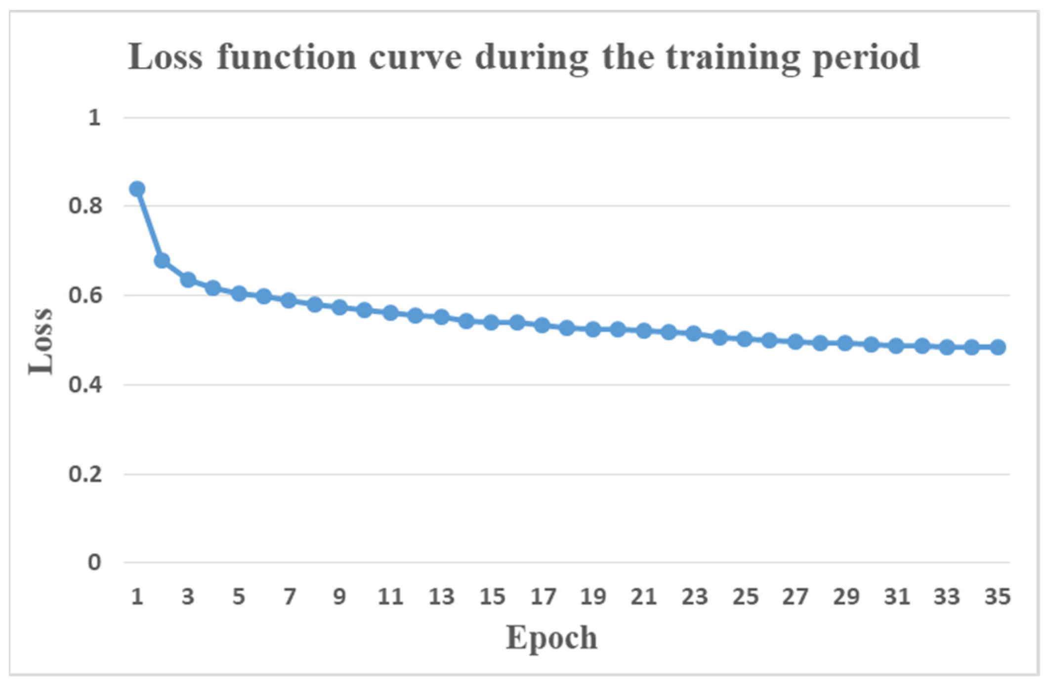
The loss function curve of the proposed model during the training period is shown in Figure 9. It is clear that the model can effectively converge.

Experiment Analysis: Both quantitative and qualitative evaluations with well-known baseline approaches were conducted.

Table 5. Image quality comparisons of radar echo prediction.

MODEL	SSIM (One-Hour Prediction) ↑	SSIM (Two-Hour Prediction) ↑
OpticalFlow [17] (ROVER)	0.616	0.577
Pysteps [23] (Extrapolation)	0.626	0.589
Pysteps [23] (S-PROG)	0.678	0.645
ConvLSTM [9]	0.634	0.579
PredRNN++ [37]	0.676	0.648
STPNet	0.675	0.654
2S-STRef	0.694	0.665

shows the SSIM results of the seven models on the one-hour prediction and two-hour prediction. In this table, ‘↑’ means the higher value is better.

From this table, all the deep learning models outperform the optical flow-based ROVER algorithm [17]. Both the extrapolation method and deterministic nowcast method with S-PROG in Pysteps [23] also obtain a better SSIM performance than ROVER [17]. Note that the deterministic nowcast method with S-PROG can achieve sharp prediction and better SSIM performance even than some deep leaning methods. Among the deep learning models, the performance of ConvLSTM is unsatisfactory. The STPNet (0.675, the first stage of our model) achieves a similar result to the PredRNN++ model (0.676) on the one-hour prediction, whereas the proposed 2S-STRef performs the best and improves the SSIM score of PredRNN++ from 0.675 to 0.693 (increase by 2.5% on the one-hour prediction), and from 0.648 to 0.665 (increase by 2.62% on the two-hour prediction). Compared with the STPNet, it is also 0.018 higher, increased by 2.67% on the one-hour prediction. It further shows that the proposed second-stage refinement model RefNet is beneficial to generate sharper meteorological imagery predictions with more details.

Furthermore, the prediction accuracies by these methods were evaluated using several widely used precipitation nowcasting metrics. To make a fair comparison and full appreciation of the algorithms’ performance, we also calculated CSI, HSS, POD, and FAR over different radar reflectivity thresholds, including 20 dBZ (about 0.5 mm/h), 35 dBZ, and 45 dBZ.

Table 6. Skill score at R > 20 dBZ (two-hour prediction).

MODEL	CSI ↑	HSS ↑	POD ↑	FAR ↓
OpticalFlow [17] (ROVER)	0.490	0.563	0.627	0.322
Pysteps [23] (Extrapolation)	0.480	0.554	0.600	0.312
Pysteps [23] (S-PROG)	0.501	0.578	0.620	0.293
ConvLSTM [9]	0.552	0.645	0.725	0.289
PredRNN++ [37]	0.576	0.653	0.731	0.277
STPNet	0.584	0.663	0.728	0.259
2S-STRef	0.588	0.665	0.747	0.272

,

Table 7. Skill score at R > 35 dBZ (two-hour prediction).

MODEL	CSI ↑	HSS ↑	POD ↑	FAR ↓
OpticalFlow [17] (ROVER)	0.317	0.441	0.455	0.519
Pysteps [23] (Extrapolation)	0.315	0.438	0.442	0.512
Pysteps [23] (S-PROG)	0.326	0.452	0.458	0.502
ConvLSTM [9]	0.352	0.508	0.602	0.510
PredRNN++ [37]	0.378	0.513	0.611	0.516
STPNet	0.393	0.530	0.626	0.500
2S-STRef	0.398	0.536	0.611	0.480

and

Table 8. Skill score at R > 45 dBZ (two-hour prediction).

MODEL	CSI ↑	HSS ↑	POD ↑	FAR ↓
OpticalFlow [17] (ROVER)	0.129	0.212	0.207	0.772
Pysteps [23] (Extrapolation)	0.133	0.214	0.209	0.768
Pysteps [23] (S-PROG)	0.127	0.198	0.197	0.789
ConvLSTM [9]	0.166	0.277	0.319	0.743
PredRNN++ [37]	0.184	0.296	0.362	0.740
STPNet	0.192	0.308	0.373	0.728
2S-STRef	0.195	0.312	0.373	0.721

show the precipitation nowcasting metric results for the two-hour prediction. $R \ge \tau$ denotes the skill score at the τ dBZ echo reflectivity threshold.

In these tables, ‘↑’ means the higher value is better, and ‘↓’ means the lower value is better. The best result is also marked with bold face. It can be found that among the typical models, the OpticalFlow-based ROVER [17] method and two methods in Pysteps [23] (extrapolation method and deterministic nowcast with S-PROG) have relatively poor prediction performance, and there is a gap in the evaluation indices compared with the deep learning models. Moreover, the extrapolation method in Pysteps [23] can obtain a similar prediction performance with the OpticalFlow-based ROVER [17] method. Compared with the ROVER method, deterministic nowcast with S-PROG in Pysteps [23] can achieve better nowcasting scores at the 20 dBZ and 35 dBZ thresholds. For the heavy precipitation (45 dBZ), its prediction performance decreases more. In deep learning approaches, the nonlinear and convolutional structure of the network is able to learn some complex spatiotemporal patterns in the dataset. However, updating the future flow fields reasonably is hard in the optical flow-based methods. Next, we focus on the three competitive methods (PredRNN++, STPNet, and 2S-STRef) and compare their performances. It is clear that the proposed 2S-STRef or STPNet achieves better nowcasting scores than PredRNN++ for all the four precipitation nowcasting metrics, and especially has an obvious improvement at the 35 dBZ (5 mm/h) and 45 dBZ (30 mm/h) thresholds. At the 45 dBZ echo threshold, the CSI of the proposed 2S-STRef is over 0.066 higher than that of the OpticalFlow-based ROVER method (increase by about 51%), and also 0.011 higher than that of the PredRNN++ model (increase by nearly 6%). Additionally, the HSS is much improved, by about 47% than that of the OpticalFlow-based ROVER method, and by over 5.4% than that of the PredRNN++ method. It means that the proposed method has better prediction performance for heavy rainfall, which is usually a difficult task. In addition, compared with those of STPNet (the first stage of our model), besides the SSIM index, the four important precipitation nowcasting metric performances of the proposed 2S-STRef are also more excellent. It is verified that the proposed RefNet (the second stage of our model) effectively improves the prediction image details and enhances nowcasting accuracy.

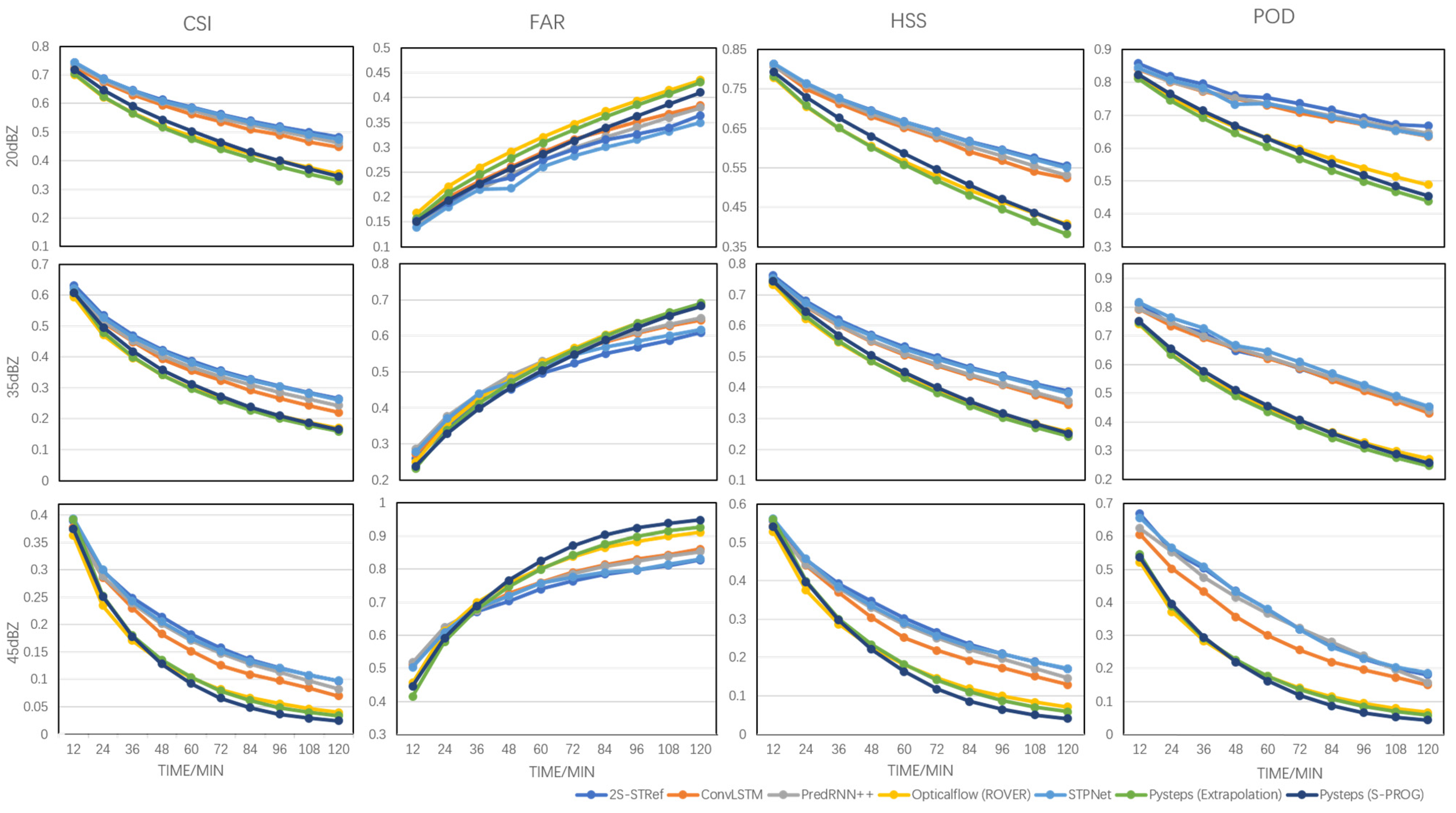
Furthermore, the precipitation nowcasting metric scores for the 12- to 120-min lead times are shown in Figure 10 for a more complete performance verification. The results in Figure 10 and Figure 11 are the average scores for the whole test dataset. In this part, extrapolation nowcast and deterministic nowcast with S-PROG in Pysteps [23] are also added for comparison. Extrapolation nowcast using a local tracking approach (Lucas–Kanade) with default configurations in Pysteps [23] is utilized in this paper. This configuration makes the performance of Pysteps (Extrapolation) similar to the OpticalFlow-based ROVER method. At the 20 dBZ and 35 dBZ thresholds, Pysteps (S-PROG) has better prediction performance than Pysteps (Extrapolation) and the OpticalFlow-based ROVER method. However, its nowcasting performance degrades faster at the 45 dBZ threshold as the lead time increases. Moreover, from this figure, it is clear that the deep learning method outperform the OpticalFlow-based ROVER method [17], Extrapolation, and S-PROG nowcasts in Pysteps [23], as the lead time increases.

The increasing rate curves comparing the proposed 2S-STRef with PredRNN++ and STPnet are presented in Figure 11. From this figure, the proposed 2S-STRef has significant accuracy improvement compared with PredRNN++, especially for the important CSI and HSS metrics. Moreover, the second-stage network RefNet can further enhance the forecasting accuracy for the 12- to 120-min lead times.

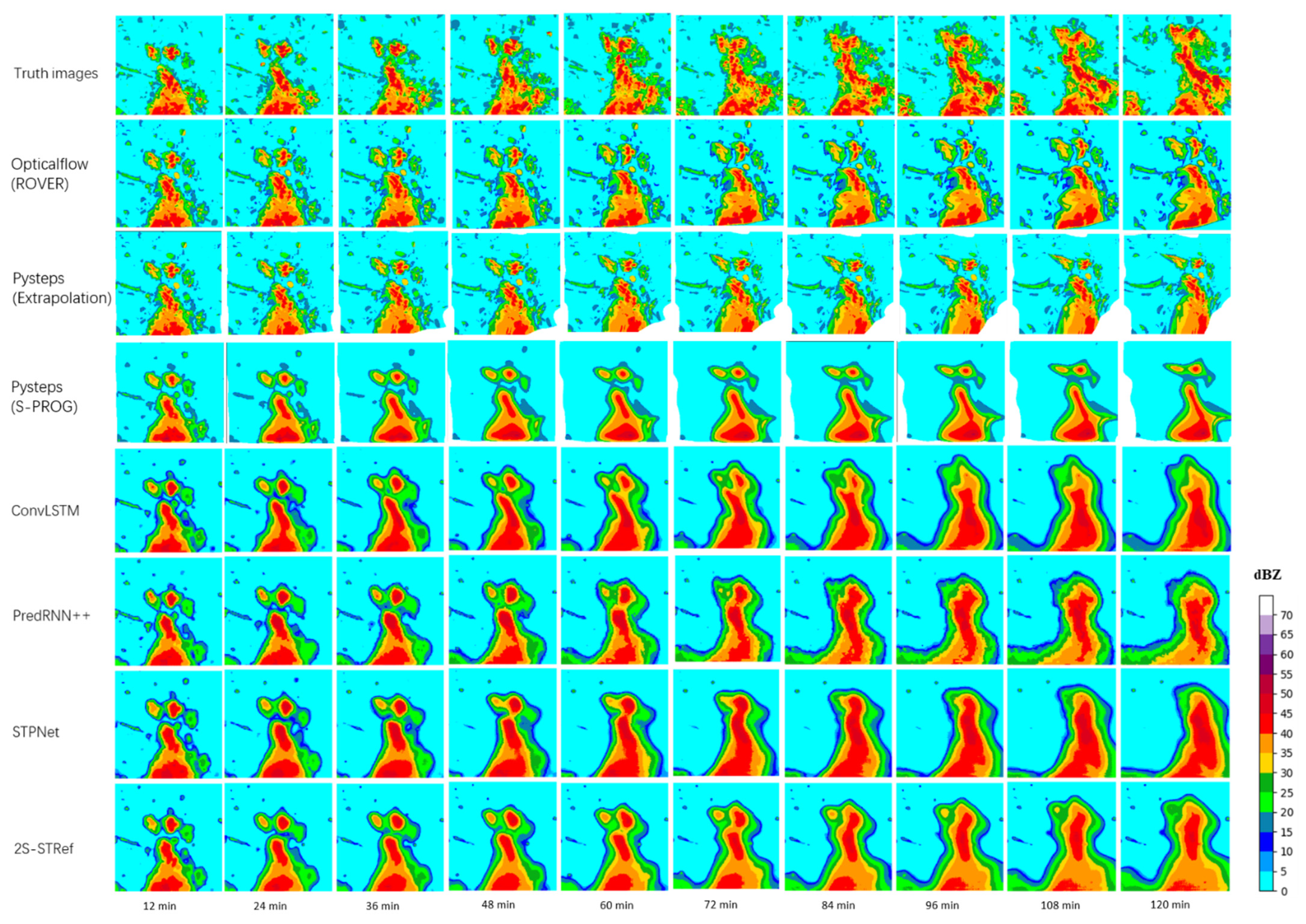
In addition, visualization of the comparison among the evaluated methods is shown in Figure 12. Although the OpticalFlow-based ROVER method [17], extrapolation nowcast, and deterministic nowcast with S-PROG in PySteps [23] can give sharper predictions than the deep learning methods, they trigger more false alarms and are less precise than deep learning methods in general. Moreover, the small-scale details in extrapolations by deep learning methods are gradually lost and the boundaries become smooth as the lead time increases. Deep blue contours in deep learning methods are actual predicted values by the network and are not processed manually. The blurring effect of deep learning methods may be caused by the inherent uncertainties of the task. Since sharp and accurate predictions of the whole radar maps in longer-term predictions are quite difficult, blurring the predictions to alleviate the error and decrease the MAE or MSE-based loss caused by this type of uncertainty is utilized. Thus, more effective loss functions can be tried and designed to improve the quality of the nowcast images in the future work.

4. Conclusions

In this paper, 2S-STRef was proposed for precipitation nowcasting by radar echo extrapolation. The first stage is STPNet using the encoder-decoder structure, which extracts the dynamic spatial and temporal correlations in a sequence of radar echo images and outputs a first-stage prediction. In the second stage, the RefNet is proposed, employing multi-scale feature extraction and fusion residual block to acquire a better performance on details and prediction accuracy of the nowcasting radar echo images. Experimental results from a real-world radar echo of South China dataset demonstrated that the proposed 2S-STRef method outperforms the conventional OpticalFlow, PySteps methods, and ConvLSTM and PredRNN++ methods on both image quality evaluation and forecasting evaluation metrics. The radar echo images predicted by the proposed network present more details and accomplish higher prediction accuracy.

The challenges are that sharp and accurate predictions of the whole radar maps in longer-term predictions are quite difficult.

The limitation of such a deep learning method is that:

• The input and output dimensions of the model are fixed, and it does not deal with length or dimension variant input sequences. If different input numbers or input dimensions of radar echo maps are input, the model must be redesigned and retrained.
• The lack of explainability of deep learning models should be improved.

Future research should investigate:

• Developing new models to further improve the prediction accuracy as well as enhance the predicted details of the radar echo images, especially for heavy rainfall.
• Since the lifetime of radar echo is finite, the predictability of radar echoes gradually deteriorates over time. When the lead time exceeds the echo lifetime, it is hard to predict the future radar echo in the initial state only based on radar data. Other meteorological parameters, such as wind, should be introduced into the extrapolation model in the future to improve the prediction accuracy of radar echo change and further increase the lead time of radar extrapolation.
• More radar echo reflectivity images in summer and winter periods will be selected and used to train the proposed network separately to enhance the prediction accuracy, since the physics and evolution behind each type is not the same.
• We will also try to build an operational nowcasting system using the proposed algorithm.

References

- Gneiting, T.; Raftery, A.E. Weather forecasting with ensemble methods. Science 2005, 310, 248–249. [Google Scholar] [CrossRef] [PubMed] [Green Version]
- Jones, N. Machine learning tapped to improve climate forecasts. Nature 2017, 548, 379–380. [Google Scholar] [CrossRef] [PubMed]
- Schmid, F.; Wang, Y.; Harou, A. Nowcasting guidelines—A summary. In WMO-No. 1198; World Meteorological Organization: Geneva, Switzerland, 2017; Chapter 5. [Google Scholar]
- Shi, X.; Gao, Z.; Lausen, L.; Wang, H.; Yeung, D.Y.; Wong, W.K.; Woo, W.C. Deep learning for precipitation nowcasting: A benchmark and a new model. In Proceedings of the 30th International Conference on Neural Information Processing Systems (NeurIPS), Long Beach, CA, USA, 4–9 December 2017; pp. 5617–5627. [Google Scholar]
- Bromberg, C.L.; Gazen, C.; Hickey, J.J.; Burge, J.; Barrington, L.; Agrawal, S. Machine learning for precipitation nowcasting from radar images. In Proceedings of the Machine Learning and the Physical Sciences Workshop at the 33rd Conference on Neural Information Processing Systems (NeurIPS), Vancouver, BC, Canada, 8–14 December 2019; pp. 1–4. [Google Scholar]
- Qiu, M.; Zhao, P.; Zhang, K.; Huang, J.; Shi, X.; Wang, X.; Chu, W. A short-term rainfall prediction model using multi-task convolutional neural networks. In Proceedings of the IEEE International Conference on Data Mining, New Orleans, LA, USA, 18–21 November 2017; pp. 395–404. [Google Scholar]
- Bouget, V.; Béréziat, D.; Brajard, J.; Charantonis, A.; Filoche, A. Fusion of rain radar images and wind forecasts in a deep learning model applied to rain nowcasting. Remote Sens. 2021, 13, 246. [Google Scholar] [CrossRef]
- Ham, Y.G.; Kim, J.H.; Luo, J.J. Deep learning for multi-year ENSO forecasts. Nature 2019, 573, 568–572. [Google Scholar] [CrossRef]
- Shi, X.; Chen, Z.; Wang, H.; Yeung, D.Y.; Wong, W.K.; Woo, W.C. Convolutional LSTM network: A machine learning approach for precipitation nowcasting. In Proceedings of the 28th International Conference on Neural Information Processing Systems (NeurIPS), Montreal, QC, Canada, 7–12 December 2015; pp. 802–810. [Google Scholar]
- Marchuk, G. Numerical Methods in Weather Prediction; Elsevier: Amsterdam, The Netherlands, 2012. [Google Scholar]
- Tolstykh, M.A.; Frolov, A.V. Some current problems in numerical weather prediction. Izv. Atmos. Ocean. Phys. 2005, 41, 285–295. [Google Scholar]
- Juanzhen, S.; Ming, X.; James, W.W.; Zawadzki, I.; Ballard, S.P.; Onvlee-Hooimeyer, J.; Pinto, J. Use of NWP for nowcasting convective precipitation: Recent progress and challenges. Bull. Am. Meteorol. Soc. 2014, 95, 409–426. [Google Scholar]
- Crane, R.K. Automatic cell detection and tracking. IEEE Trans. Geosci. Electron. 1979, 17, 250–262. [Google Scholar] [CrossRef]
- Rinehart, R.E.; Garvey, E.T. Three-dimensional storm motion detection by conventional weather radar. Nature 1978, 273, 287–289. [Google Scholar] [CrossRef]
- Bowler, N.E.; Pierce, C.E.; Seed, A. Development of a precipitation nowcasting algorithm based upon optical flow techniques. J. Hydrol. 2004, 288, 74–91. [Google Scholar] [CrossRef]
- Bellon, A.; Zawadzki, I.; Kilambi, A.; Lee, H.C.; Lee, Y.H.; Lee, G. McGill algorithm for precipitation nowcasting by lagrangian extrapolation (MAPLE) applied to the South Korean radar network. Asia-Pac. J. Atmos. Sci. 2010, 46, 369–381. [Google Scholar] [CrossRef]
- Woo, W.-C.; Wong, W.-K. Operational application of optical flow techniques to radar-based rainfall nowcasting. Atmosphere 2017, 8, 48. [Google Scholar] [CrossRef] [Green Version]
- Germann, U.; Zawadzki, I. Scale-dependence of the predictability of precipitation from continental radar images. Part I: Description of the methodology. Mon. Weather Rev. 2002, 130, 2859–2873. [Google Scholar] [CrossRef]
- Germann, U.; Zawadzki, I. Scale dependence of the predictability of precipitation from continental radar images. Part II: Probability forecasts. J. Appl. Meteorol. 2004, 43, 74–89. [Google Scholar] [CrossRef]
- Chung, K.S.; Yao, I.A. Improving radar echo Lagrangian extrapolation nowcasting by blending numerical model wind information: Statistical performance of 16 typhoon cases. Mon. Weather Rev. 2020, 148, 1099–1120. [Google Scholar] [CrossRef]
- Seed, A.W. A dynamic and spatial scaling approach to advection forecasting. J. Appl. Meteorol. 2003, 42, 381–388. [Google Scholar] [CrossRef]
- Ryu, S.; Lyu, G.; Do, Y.; Lee, G. Improved rainfall nowcasting using Burgers’ equation. J. Hydrol. 2020, 581, 124140. [Google Scholar] [CrossRef]
- Pulkkinen, S.; Nerini, D.; Pérez Hortal, A.A.; Velasco-Forero, C.; Seed, A.; Germann, U.; Foresti, L. Pysteps: An open-source Python library for probabilistic precipitation nowcasting (v1. 0). Geosci. Model Dev. 2019, 12, 4185–4219. [Google Scholar] [CrossRef] [Green Version]
- Tian, L.; Li, X.; Ye, Y.; Pengfei, X.; Yan, L. A generative adversarial gated recurrent unit model for precipitation nowcasting. IEEE Geosci. Remote Sens. Lett. 2019, 17, 601–605. [Google Scholar] [CrossRef]
- Hernández, E.; Sanchez-Anguix, V.; Julian, V.; Palanca, J.; Duque, N. Rainfall prediction: A deep learning approach. In Proceedings of the International Conference on Hybrid Artificial Intelligence Systems, Seville, Spain, 18–20 April 2016; pp. 151–162. [Google Scholar]
- Cyril, V.; Marc, M.; Christophe, P.; Marie-Laure, N. Numerical weather prediction (NWP) and hybrid ARMA/ANN model to predict global radiation. Energy 2012, 39, 341–355. [Google Scholar]
- McGovern, A.; Elmore, K.L.; Gagne, D.J.; Haupt, S.E.; Karstens, C.D.; Lagerquist, R.; Williams, J.K. Using artificial intelligence to improve real-time decision-making for high-impact weather. Bull. Am. Meteorol. Soc. 2017, 98, 2073–2090. [Google Scholar] [CrossRef]
- Wang, B.; Lu, J.; Yan, Z.; Luo, H.; Li, T.; Zheng, Y.; Zhang, G. Deep uncertainty quantification: A machine learning approach for weather forecasting. In Proceedings of the International Conference on Knowledge Discovery and data Mining (SIGKDD) 2019, Anchorage, AK, USA, 4–8 August 2019; pp. 2087–2095. [Google Scholar]
- Imam Cholissodin, S. Prediction of rainfall using improved deep learning with particle swarm optimization. Telkomnika 2020, 18, 2498–2504. [Google Scholar] [CrossRef]
- Lin, T.; Li, Q.; Geng, Y.A.; Jiang, L.; Xu, L.; Zheng, D.; Zhang, Y. Attention-based dual-source spatiotemporal neural network for lightning forecast. IEEE Access 2019, 7, 158296–158307. [Google Scholar] [CrossRef]
- Basha, C.Z.; Bhavana, N.; Bhavya, P.; Sowmya, V. Rainfall prediction using machine learning & deep learning techniques. In Proceedings of the International Conference on Electronics and Sustainable Communication Systems (ICESC), Coimbatore, India, 2–4 July 2020; pp. 92–97. [Google Scholar]
- Sapankevych, N.I.; Sankar, R. Time series prediction using support vector machines: A survey. IEEE Comput. Intell. Mag. 2009, 4, 24–38. [Google Scholar] [CrossRef]
- Sutskever, I.; Vinyals, O.; Le, Q.V. Sequence to sequence learning with neural networks. In Proceedings of the 31st International Conference on Neural Information Processing Systems (NIPS), Montreal, QC, Canada, 8–13 December 2014; pp. 3104–3112. [Google Scholar]
- Salman, A. Single layer & multi-layer long short-term memory (LSTM) model with intermediate variables for weather forecasting. Procedia Comput. Sci. 2018, 135, 89–98. [Google Scholar]
- Benjamin, K.; Lior, W.; Yehuda, A. A dynamic convolutional layer for short range weather prediction. In Proceedings of the 2015 IEEE Conference on Computer Vision and Pattern Recognition (CVPR), Boston, MA, USA, 7–12 June 2015; pp. 4840–4848. [Google Scholar]
- Wang, Y.; Long, M.; Wang, J.; Gao, Z.; Yu, P.S. PredRNN: Recurrent neural networks for predictive learning using spatiotemporal lstms. In Proceedings of the 31st International Conference on Neural Information Processing Systems, Long Beach, CA, USA, 4–9 December 2017; pp. 879–888. [Google Scholar]
- Wang, Y.; Gao, Z.; Long, M.; Wang, J.; Philip, S.Y. PredRNN++: Towards a resolution of the deep-in-time dilemma in spatiotemporal predictive learning. In Proceedings of the International Conference on Machine Learning (PMLR), Beijing, China, 14–16 November 2018; pp. 5123–5132. [Google Scholar]
- Geng, Y.; Li, Q.; Lin, T.; Jiang, L.; Xu, L.; Zheng, D.; Yao, W.; Lyu, W.; Zhang, Y. Lightnet: A dual spatiotemporal encoder network model for lightning prediction. In Proceedings of the 25th ACM SIGKDD International Conference on Knowledge Discovery & Data Mining, Anchorage, AK, USA, 4–8 August 2019; pp. 2439–2447. [Google Scholar]
- Zhang, F.; Wang, X.; Guan, J.; Wu, M.; Guo, L. RN-Net: A deep learning approach to 0–2 h rainfall nowcasting based on radar and automatic weather station data. Sensors 2021, 21, 1981. [Google Scholar] [CrossRef] [PubMed]
- Xu, Z.; Du, J.; Wang, J.; Jiang, C.; Ren, Y. Satellite image prediction relying on GAN and LSTM neural networks. In Proceedings of the IEEE International Conference on Communications (ICC), Shanghai, China, 20–24 May 2019; pp. 1–6. [Google Scholar]
- Ravuri, S.; Lenc, K.; Willson, M.; Kangin, D.; Lam, R.; Mirowski, P.; Mohamed, S. Skillful Precipitation nowcasting using deep generative models of radar. arXiv 2021, arXiv:2104.00954. [Google Scholar]
- Li, Y.; Lang, J.; Ji, L.; Zhong, J.; Wang, Z.; Guo, Y.; He, S. Weather forecasting using ensemble of spatial-temporal attention network and multi-layer perceptron. Asia-Pac. J. Atmos. Sci. 2020, 2020, 1–14. [Google Scholar] [CrossRef] [Green Version]
- Khan, M.I.; Maity, R. Hybrid deep learning approach for multi-step-ahead daily rainfall prediction using GCM simulations. IEEE Access 2020, 8, 52774–52784. [Google Scholar] [CrossRef]
- Eddy, I.; Nikolaus, M.; Tonmoy, S.; Margret, K.; Alexey, D.; Thomas, B. Flownet 2.0: Evolution of optical flow estimation with deep networks. In Proceedings of the IEEE Conference on Computer Vision and Pattern Recognition (CVPR), Honolulu, HI, USA, 21–26 July 2017; pp. 2462–2470. [Google Scholar]
- Liu, H.B.; Lee, I. MPL-GAN: Toward realistic meteorological predictive learning using conditional GAN. IEEE Access 2020, 8, 93179–93186. [Google Scholar] [CrossRef]
- Schultz, M.G.; Betancourt, C.; Gong, B.; Kleinert, F.; Langguth, M.; Leufen, L.H.; Stadtler, S. Can deep learning beat numerical weather prediction? Philos. Trans. R. Soc. A 2021, 379, 20200097. [Google Scholar] [CrossRef] [PubMed]
- Seed, A.W.; Pierce, C.E.; Norman, K. Formulation and evaluation of a scale decomposition-based stochastic precipitation nowcast scheme. Water Resour. Res. 2013, 49, 6624–6641. [Google Scholar] [CrossRef]
- Qin, J.; Huang, Y.; Wen, W. Multi-scale feature fusion residual network for single image super-resolution. Neurocomputing 2020, 379, 334–342. [Google Scholar] [CrossRef]
- Zhou, Y.; Dong, J.; Yang, Y. Deep fractal residual network for fast and accurate single image super resolution. Neurocomputing 2020, 398, 389–398. [Google Scholar] [CrossRef]
- Hu, J.; Shen, L.; Sun, G. Squeeze-and-excitation networks. In Proceedings of the IEEE Conference on Computer Vision and Pattern Recognition (CVPR), Salt Lake City, UT, USA, 18–22 June 2018; pp. 7132–7141. [Google Scholar]
- Wang, Z.; Bovik, A.C.; Sheikh, H.R.; Simoncelli, E.P. Image quality assessment: From error visibility to structural similarity. IEEE Trans. Image Process. 2004, 13, 600–612. [Google Scholar] [CrossRef] [Green Version]
- Diederik, K.; Jimmy, B. Adam: A method for stochastic optimization. arXiv 2015, arXiv:1412.6980. [Google Scholar]
- Hansoo, L.; Sungshin, K. Ensemble classification for anomalous propagation echo detection with clustering-based subset-selection method. Atmosphere 2017, 8, 11. [Google Scholar]
- Song, K.; Yang, G.; Wang, Q.; Xu, C.; Liu, J.; Liu, W.; Zhang, W. Deep learning prediction of incoming rainfalls: An operational service for the city of Beijing, China. In Proceedings of the 2019 International Conference on Data Mining Workshops (ICDMW), Beijing, China, 8–11 November 2019; pp. 180–185. [Google Scholar]
Figure 1.
An example of radar echo image in the Southern China (around Guangzhou City) at 6 March 2021 00:00(UTC).
Figure 2.
The overall architecture of our 2S-STRef network, which is composed of two stages including the spatiotemporal prediction stage and detail refinement stage. Detailed structure parameters can be found in Table 1 and Table 2.
Figure 3.
The encoder structure of STPNet, including three stacked ST-RNN layers and downsampling layers.
Figure 4.
The decoder structure of STPNet, including three stacked ST-RNN layers and upsampling layers.
Figure 5.
Predicted radar echo image with the lead time: 12 min (a) ground truth; (b) with the STPNet method. The radar echo images are of Southern China (around Guangzhou City) at 31 March 2019.