
Time-Series Landsat Data for 3D Reconstruction of Urban History


1
State Key Laboratory of Urban and Regional Ecology, Research Center for Eco-Environmental Sciences, Chinese Academy of Sciences, Beijing 100085, China
2
College of Resources and Environment, University of Chinese Academy of Sciences, Beijing 100049, China
3
Beijing Urban Ecosystem Research Station, Research Center for Eco-Environmental Sciences, Chinese Academy of Sciences, Beijing 100085, China
4
Beijing-Tianjin-Hebei Urban Megaregion National Observation and Research Station for Eco-Environmental Change, Research Center for Eco-Environmental Sciences, Chinese Academy of Sciences, Beijing 100085, China
5
State Environmental Protection Scientific Observation and Research Station for Ecology and Environment of Rapid Urbanization Region, Shenzhen Environmental Monitoring Center, Shenzhen 518049, China
*
Author to whom correspondence should be addressed.
Remote Sens. 2021, 13(21), 4339; https://0-doi-org.brum.beds.ac.uk/10.3390/rs13214339
Submission received: 11 September 2021
/
Revised: 21 October 2021
/
Accepted: 26 October 2021
/
Published: 28 October 2021
(This article belongs to the Special Issue Smart City Development and Remote Sensing Application in Urban Ecology)
Abstract
:Accurate quantification of vertical structure (or 3D structure) and its change of a city is essential for understanding the evolution of urban form, and its social and ecological consequences. Previous studies have largely focused on the horizontal structure (or 2D structure), but few on 3D structure, especially for long time changes, due to the absence of such historical data. Here, we present a new approach for 3D reconstruction of urban history, which was applied to characterize the urban 3D structure and its change from 1986 to 2017 in Shenzhen, a megacity in southern China. This approach integrates the contemporary building height obtained from the increasingly available data of building footprint with building age estimated based on the long-term observations from time-series Landsat imagery. We found: (1) the overall accuracy for building change detection was 87.80%, and for the year of change was 77.40%, suggesting that the integrated approach provided an effective method to cooperate horizontal (i.e., building footprint), vertical (i.e., building height), and temporal information (i.e., building age) to generate the historical data for urban 3D reconstruction. (2) The number of buildings increased dramatically from 1986 to 2017, by eight times, with an increased proportion of high-rise buildings. (3) The old urban areas continued to have the highest density of buildings, with increased average height of buildings, but there were two emerging new centers clustered with high-rise buildings. The long-term urban 3D maps allowed characterizing the spatiotemporal patterns of the vertical dimension at the city level, which can enhance our understanding on urban morphology.
1. Introduction
Rapid urbanization is increasingly becoming one of the most pressing issues worldwide [1,2]. With massive population moving into cities, the cities tend to grow more vertically in addition to outward expansion [3,4]. Such changes in urban form have remarkable social and ecological consequences, and thereby urban sustainability [4,5,6,7]. Numerous studies have been conducted to characterize urban form and its change from a horizontal (i.e., 2D) perspective, and to examine the social and ecological impacts [8,9,10,11,12,13]. However, while the importance of the vertical dimension (i.e., 3D) of a city has been widely recognized, far fewer studies have been conducted from the vertical dimension perspective, with a few exceptions [14,15,16,17]. This is largely due to the lack of historical data that can be used to quantify the 3D structure of cities. It is important, therefore, to develop approaches that can accurately quantify vertical structure (or 3D structure) and its change of a city.
With the wide availability of Light Detection and Ranging (LiDAR) data and the satellite and airborne stereo imagery, Digital Elevation Models (DEMs) and Digital Surface Models (DSMs) can be obtained at a large spatial extent for urban 3D structure study [18,19,20,21]. Recently, the building footprints with the height attribute, typically measured as the number of floors, have been increasingly available for many cities [16,17,22]. Based on the data mentioned above, the spatial pattern of vertical structure can be characterized by building physical indexes such as building height and volume, and building geometry, such as density, surface roughness, sky view factor, and canopy breadth ratio [4,15,23,24]. However, such data in general only include contemporary information of buildings. Without the information of building age (i.e., when the buildings were built), we are not able to quantitatively examine the changes in the 3D structure of cities, as what is frequently carried out for the 2D structure of cities.
Integrating the contemporary information of building height with the temporal information of building age detected based on long-term observations from time-series remotely sensed imagery may provide an effective method to address this issue. Facilitated by the archive opening and the technological advances in data storage and processing, numerous studies have been conducted to develop approaches to identify when the land cover change occurs by using time-series Landsat or Sentinel imagery [25,26,27,28]. Using this temporal information, such as when cropland was abandoned and re-cultivated [29] or when forest was recovered from pest disease and/or fire disturbance [30], appropriate management strategies of vegetation can be developed. These approaches were also applied to identify the year when urban expansion occurred [31,32] and to examine the trajectories of impervious surface cover [33]. While few studies have been conducted to directly identify when buildings were constructed, there are a few studies based on similar topics. For example, Uhl and Leyk (2019) conducted built-up area change analysis based on Landsat time-series data, using building footprints as spatial constrained [34]. Huang et al. (2020) and Wen et al. (2019) used time-series satellite images with a very high spatial resolution to detect newly constructed building areas [35,36]. Such successful cases indicated that the integration of contemporary building height with change detection on building age using long-term observations from time-series remotely sensed data has the potential for urban 3D reconstruction.
In this study, we present a new approach for 3D reconstruction of urban history, which was applied to characterize the urban 3D structure and change, using the city of Shenzhen as a case study. This approach integrates the contemporary building footprint with long-term time-series Landsat imagery. Specifically, the objectives are to: (1) develop a new approach that can be used for 3D reconstruction of urban history; (2) test the new approach in the megacity of Shenzhen and investigated the spatiotemporal patterns of the 3D structure of the city from 1986 to 2017.
2. Study Area and Data
2.1. Study Area
We selected Shenzhen, a megacity in southeast coastal China to test our approach. Shenzhen consists of ten urban districts and has an area of 1997 km2 (Figure 1). It has a total population of 13.43 million in 2019, with a population density of 6,729 person/km2. Developed land in Shenzhen has been expanding dramatically since the later 1970s. The size of developed land in 2017 was more than 30 times to that in the1970s [37]. Additionally, Shenzhen also grew dramatically in the vertical dimension [38]. Building density, shape, height, and spatial configuration varied greatly in Shenzhen, showing remarkable spatial heterogeneity (Figure.1). Such diversity and complexity of buildings in Shenzhen make it ideal to test our approach.
2.2. Data
2.2.1. Annual Landsat Imagery and Land Cover Maps
We estimated the year in which the building was built (i.e., building age) based on annual time-series land cover maps from 1986 to 2017, generated using time-series Landsat imagery acquired in 1986–2017. These maps included four land cover types, vegetation, water, developed land, and barren land, and the overall accuracies of them ranged from 88.00% to 95.50% [39]. For the map generation, we first acquired the Landsat TM, ETM+, and OLI imagery which covers the path/row of 122/44 and 121/44 by referencing the Worldwide Reference System-2 (WRS-2) from the United States Geological Survey (USGS). We then selected 68 scenes with cloud cover under 10% and mosaicked the imagery to obtain the annual Landsat data which covers the entire study area. In order to reduce the seasonal impacts caused by cloud cover removal and make the most use of each scene, we generated the time-series of maximum Normalized Difference Vegetation Index (NDVI) on the Google Earth Engine (GEE) platform (https://earthengine.google.com/, accessed on 30 September 2021) and used them as auxiliary data. The land cover map for each year was generated using the random forest classifier which the maximum number of resulting decision trees was 100 and the active variable for determining the best splits for each tree was 3 [40,41].
2.2.2. Building Footprint
The building footprint in 2017 with height attribute, formatted in a vector layer, was obtained from the Bureau of Planning and Natural Resources in Shenzhen. This data, generated by photogrammetry and field investigation [42], covers the entire city of Shenzhen and contains approximately 567,000 buildings. We classified the buildings into four types according to the standard from the Code for Design of Civil Buildings, including low-rise building (1–3 stories), multi-story building (4–6 stories), middle-rise building (7–9 stories), and high-rise building (≥10 stories). The percentages of the four types of buildings were 51.9%, 31.0%, 12.5%, and 4.5% in 2017, respectively. We also collected the transportation network in 2017 from the Open Street Map, which was used to generate the analysis units. Such transportation network consists of highways and trunk roads at primary, secondary, and tertiary levels.
3. Method
The proposed approach for the 3D reconstruction of urban history includes two steps. First, the approach detects the constructed year (building age) for each contemporary building by change detection based on the long-term observations from the time-series Landsat imagery/land cover data and thereby generates a map of buildings with the attribute of constructed year (age). Second, the approach transfers the current building heights to the building footprint with ages for the historical 3D mapping (Figure 2). Here, we conducted the post-classification comparison for change analysis to determine the building age for each building. We additionally compared the availability of different spatial units because we found buildings in a city varied greatly in size, with some smaller than a pixel with a spatial resolution of 30 m and some covering several pixels. We then chose the unit with the best accuracy on building age estimation and applied the approach to characterize the spatiotemporal pattern of urban 3D structures from 1986 to 2017 in Shenzhen.
3.1. Change Detection for Building Age Estimation
Two methods, post-classification comparison and pre-classification change detection, can be used to detect the developed land change and then identify the year in which the building was built [43,44,45]. Here, we used the post-classification comparison for change detection. We first calculated the time series of fractional land cover (TSFLC) for every land cover type in each analysis unit and constructed the land cover trajectories. We then segmented the time-series into fragments based on the TSFLC change magnitude and detected the land cover change. The year in which the change occurred was recorded in this process. Here, the key step is to determine the threshold of the TSFLC change magnitude. We used two thresholds, that is, threshold b for detecting the abrupt and gradual changes of land cover, and threshold a for constraining the error generated from the land cover classification accuracy. If the TSFLC change magnitude between two neighboring years was larger than b, we considered abrupt change occurred. If cumulative change magnitude for more than two years was larger than b, we considered gradual change. More details can be found in Jing et al. (2021) [39]. As we focused on the building change in this study, the fractional changes of developed land were used to identify the constructed year, which is to capture the latest year of the developed land change.
Different spatial units, such as street block, parcel, and pixel, have been used to detect the land cover change and then identify the timing of the occurrence of change [33,46,47,48]. Buildings in a city can vary greatly in size, ranging from smaller than the size of a Landsat TM/ETM+/OLI pixel (i.e., 30 m) to containing quite a few pixels (Figure 3c). Therefore, the choice of analysis unit may affect the accuracy of change detection. Consequently, we compared the impact of different analysis units on the accuracy of change detection to choose the appropriate analytical unit. Specifically, we tested the approach using four different units, including street block, building group, single building, and pixel (Figure 3a,b) and validated the accuracies of age estimation.
Street blocks, labeled as Unit 1, are commonly considered the basic management units in urban areas. Here, we generated Unit 1 by the transportation network in 2017 and the values of a and b were 2% and 20%, respectively [33]. The building group, labeled as Unit 2, was determined by buildings with the same height in a street block and the threshold a and b were set as 10% and 50% [49,50]. The single building was labeled as Unit 3 and the thresholds of a and b were also set as 10% and 50%, respectively. A pixel, labeled as Unit 4, is the basic unit of land cover maps and there is no fractional change. Consequently, the values of a and b were 0 and 100%, respectively. Once the constructed year of each unit was determined, the timing information was aggregated to the buildings, except for the unit of a single building.
3.2. Accuracy Assessment
We used two matrices to assess the accuracies of change detection, including accuracy on building position (spatial accuracy) and that on building age (temporal accuracy). We first evaluated the accuracy of distinguishing change from no change because buildings that were constructed before 1986 had existed. We then validated the accuracies of the building age estimation by comparing the observed year and reference year of building construction [46]. We randomly sampled 1000 buildings in the method testing area by the stratified random sampling method and then implemented the visual interpretation by referencing the Landsat images, the very high-resolution historical imagery from Google Earth, and the LianjiaTM, a housing market platform for the building age validation.
3.3. Urban 3D Reconstruction
After estimating the building ages, we further transferred the current building height to the building footprint with different ages for the historical data generation. Here, we introduced the building footprint with height attribute in 2016 as an example. Based on the building age map in 1986–2017, we removed the buildings that were built after 2016 and then transferred the contemporary building height, acquired from the building footprint with height attribute in 2017, to generate the 3D map in 2016. We then generated the annual 3D maps in 1986–2015 by the same method and statistically analyzed the spatiotemporal pattern of the 3D structure by two basic indices, building number and building height.
4. Results
4.1. Comparisons of Change Detection for Building Age Estimation
A comparison of the results from the accuracy assessment showed that the change detection using Unit 2, building group, achieved the highest overall accuracy in distinguishing change from no-change, as well as the best user’s accuracy and producer’s accuracy, with values of 87.80%, 87.20%, and 90.17%, respectively (Table 1). For the change detection using the other three units, the overall accuracies were greater than 84.00%. The user’s accuracies of change for Unit 1 and 3 were close (83.36% and 83.39%, respectively), whereas that for Unit 4 was slightly lower (81.68%), suggesting these three units were less able to identify the spatial information on building location, compared with Unit 2.
However, the temporal accuracies of building age estimation varied greatly when using different units of analysis (Figure 4). The building-based validation between the visually interpreted reference and the change detected revealed that Unit 2 had the highest overall accuracy on building age identification, with the value of 77.40% (two-year tolerance), which was higher than that by the other units, with the overall accuracies of 69.40%, 71.30%, and 68.60%, respectively (Figure 4). The error matrix displayed by the bubble chart also revealed that the proportion of those yearly producer’s accuracy below 50% was nearly 40%; that is, the samples emerged below the diagonal in the matrix, suggesting all of the units caused many omission errors on building age estimation. Comparatively, except for the omission errors, the user’s accuracies from Unit 3 and 4 were also lower, indicating the commission errors occurred at the same time when using the single building and the pixel as units of analysis to identify building age (Figure 4c,d).
Comparing the building age maps generated by the change detection using the four units in the testing area, the spatial patterns were similar, in which the relatively new buildings appeared along with the urban expansion from the west to the east (Figure 5). However, the details varied by different unit sizes. The building age from the street block and the building group were similar, but the street block had more homogenous timing information. The ages identified by the single building and pixel were more heterogeneous, which the buildings in the group with the same roof shape and height were identified as having different constructed years (Figure 5). For example, building construction years in the same residential area were identified as 1986, 1991, 1994, 1999, and 2009.
We update the building age attribute for each building based on the approach that used building group as the analysis unit. Results showed that older buildings that were constructed before the 1990s largely clustered in the Luohu district, with some old buildings dispersed in the western coastal regions (Figure 6). In contrast, the relatively new buildings that were constructed after the 2010s were distributed in the northeast and northwest of the city. The results also demonstrated the detailed representation of the settlement structure in which the old buildings were more crowded, whereas those were primarily new buildings that had more open space (Figure 6a,b).
4.2. Spatiotemporal Patterns of the 3D Structure in Shenzhen
The number of buildings in Shenzhen increased dramatically from 71,000 in 1986 to 567,000 in 2017, but with varied rates of increase during different periods. The annual growth rate in number of buildings was 3.3% in 1986–1990, but dramatically increased to 18.3% in 1990–1995, and then reached the highest value of 24.5% in 1995–2000. After the year 2000, the growth rate showed a slowdown trend, with an annual growth rate of 6.7% in 2000–2005, 2.6% in 2005–2010, and 1.7% in 2010–2017, respectively (Figure 7a).
Shenzhen was dominated by low-rise buildings, but the percentage of low-rise buildings decreased from 62.1% in 1986 to 51.9% in 2017. The percentage of middle-rise buildings also exhibited a similar change: change decreased from 15.6% in 1986 to 12.5% in 2017. In contrast, the percentage of the multi- and high-rise buildings increased from 19.8% in 1986 to 31.0% in 2017, and 2.5% to 4.5%, respectively. The average value of building height increased from 10.8 m to 12.3 m in 1986–2017, but the change magnitude of the new buildings between two neighboring years varied from different periods. The newly constructed buildings in 2007–2017 were higher than those in the other periods, with average values from 13.7 m to 28.0 m (Figure 7b).
The average of building height smoothly increased in the entire city, but with great variations in space and time. Changes in building height showed that urban form in Shenzhen shifted from a single center to multiple centers (Figure 8). The contemporary building height in 2017 exhibited a highly spatial heterogeneity, with the high-rise and middle-rise buildings mostly clustered in four regions, including location 1 in the Luohu and Futian districts, location 2 in the Nanshan district, location 3 in the Longgang district, and location 4 in the Longhua district, and the low-rise buildings dominantly distributed in the northwestern and northeastern areas of Shenzhen (Figure 8). However, in the 1980s, there was only one center located in the Luohu district, the oldest urban area in Shenzhen (Figure 6 and Figure 8). Comparing the maps of building height in 1986–2017, the creation of these four centers was corresponding with the urban growth process (Figure 8). The changes in the building height also showed that the buildings in older urban areas were higher than those in new urban areas.
5. Discussion
5.1. The Approach Reliability for 3D Reconstruction of Urban History
The results indicated that change detection using building group as the unit of analysis provided an effective method to estimate the building age, with the overall accuracy of 87.80% for building location identification and 77.40% for building age estimation (Table 1 and Figure 4). In this study, the accuracy of change detection depends on the change magnitude calculated from the developed land proportion within the analysis unit. We found the size and shape of building footprint varied greatly within the city, with some of them covering several pixels whereas others were smaller than one pixel (Figure 3). Consequently, it is crucially important to select the appropriate unit for analysis, in which the annual developed land with a spatial resolution of 30 m would be aggregated to the analytical unit to identify the building age.
First, using a fixed unit, especially an object-based unit without considering the boundary change, to measure the imagery spectral/land cover over time will cause partial change on the space within a unit during the process of land cover change [51,52]. Such partial change within a unit flatted the abrupt changes on the imagery spectral/land cover trajectory and thus fuzzed the change magnitude for the change detection [28,47,48]. When using the block as the unit, once the magnitude of developed land reached the threshold b, the timing information was recorded and then was assigned to all of the buildings inside the block, including those were built later than the year where changes were identified. This would result in omission errors for building age estimation (Table 1, Figure 4a). Although the gradual change was also considered in the change detection process, the variations of the block size reduced the change detection ability of a fixed threshold. Comparatively, grouping buildings within a block can reduce the unit size and then improve the impact from the partial change. Additionally, unlike a street block, it consists of several groups that might be constructed in different periods; the building group that was used as unit of analysis in this study is likely to be built in the same time [35]. Consequently, using building group as a unit to identify the time of change can effectively reduce omission errors (Table 1, Figure 3 and Figure 4b).
However, continually reducing the unit size does not result in higher temporal accuracy on building age estimation (Table 1 and Figure 4). Although the pixel-based change detection has been successfully used for capturing the time of land cover change [53,54], its application to identify the building age was not very successful because the trajectory of developed land proportion in a single building polygon, overlaying across pixels, are fluctuant when the sources of annual land cover maps are imprecise. Such temporal inconsistency significantly affects the temporal segmentation on the trajectory of land cover proportion by simply setting a certain threshold [33]. As a result, numerous omission and commission errors occurred at the same time when using the single building, as well as the pixel, to identify the building age. This problem, however, can be largely eliminated by the building group because enlarging the unit size allowed us to temporally smooth the time series of continuous products, and then remove such noise.
Relatively few studies investigate the changes of urban 3D structure at the city level largely due to the limitation of data availability. In this study, the approach provides an effective method to incorporate the contemporary building height with the year in which the building was built, and thereby generates the historical maps for the urban 3D structure (Figure 5 and Figure 6, and Figure 8). The building age can be considered as an intermediate to reconstruct the urban 3D history, although the Landsat data cannot provide the vertical information. The advantages of long-term observation, temporal density, and ready availability from the Landsat satellite and the increasing availability of building footprint/cadastral parcel greatly improve the application of this integrated approach. Although the historical building footprints with height information can be derived from the dataset of LiDAR, DEM, and nDSM alone, the data preprocessing is expensive, complicated, and time consuming compared with the integrated approach presented in this study. More importantly, such a dataset is often not available in most of the cities worldwide.
The integrated approach presented in this study also has limitations caused by some uncertainties. First, the unit of building groups was only determined by the building height, without considering the geometrical characteristic. The buildings can be very different in shape, structure, and their use, with buildings having similar typological characteristics being likely to have the same ages [35,50]. Consequently, more indicators, especially the morphology-based indicators, might be useful to help identify building groups. Second, the approach did not consider the building demolition and replacement so that the 3D reconstruction of urban history can only represented the change of the buildings that still exist today. Several studies revealed that many megacities in China have been shifting the urban growth model from outward expansion to internal optimization, with older buildings’ removal and replacement of impervious surfaces with greenspace [2,55]. Combining the cartographic records, such as old cadastral and topographic maps, or very-high-resolution imagery can potentially extract the missing building footprints and associated height information.
5.2. Implications of the 3D Reconstruction at City Scale
The spatiotemporal patterns of the vertical structure can be combined with the horizontal structure for further understanding of the urban form along with the urban growth. Previous studies showed a dramatic urban sprawl in the city of Shenzhen from a 2D structure perspective [56,57]. However, our results that the proportional number of low-rise buildings decreased and that of the multi- and high-rise buildings increased in 1986–2017, suggested that the urban form became more compact and thereby land use became more efficient (Figure 8). We also observed that the land use efficiency in older urban areas was higher than that in new ones, indicated by the contemporary pattern of the multi- and high-rise buildings. Such difference used to exist in the early stage of urban development although another two centers of high-rise building appeared in 2005–2017 (Figure 8). These morphological statuses and changes may be correlated to the urban planning in which the Luohu, Futian, and Nanshan districts were used to become the Special Economic Zone and the dominant functions of business and residence promoted the high-rise building construction [38].
Beyond urban expansion, the changes of urban 3D structure at the city level revealed more detailed information on the urban form. Several studies have been conducted to investigate the contemporary urban 3D structure at continental and finer scales [3,4,36]. Our results revealed similar findings that the buildings in downtown were higher. However, we also found some more details that the multiple centers clustered with high buildings emerged in new urban areas, which was quite different from the patterns in American and European cities. The fact that the first center in Shenzhen continued to have the most clustered high-rise buildings may differ from the patterns in some other Chinese cities [14].
More importantly, understanding the social and ecological consequences of the changes of vertical structure at the city level can enhance our understanding on the interactions between the anthropogenic and natural processes, which can provide insights for urban management. Previous studies revealed that the buildings with various heights shifted the landscapes from space and then resulted in negative effects on environments [15,22]. For example, the high buildings in Luohu and Futian districts turned off the corridors for migratory birds [22]. Understanding the information on how the building growth changed the bird’s movements by incorporating the historical 3D structure will support the corridor restoration. Studies have also shown positive environmental effects of the growth of 3D structures [16,58]. For example, higher buildings can increase shade for urban heat mitigation [16]. Additionally, cities growing in the vertical dimension may provide more space for greening, which may have significant benefits for human physical and mental health.
6. Conclusions
The information on urban form characterized by 3D structure and its change is essential for understanding the social and ecological effects of a city. Previously, numerous studies have focused on the change in 2D structure, but few on 3D structure, especially for long-term change due to the limitation of historical data. Here, we first developed a new approach for the 3D reconstruction of urban history and then applied it to investigate the urban 3D structure and change over time, using the city of Shenzhen as a case study. Such an approach integrates the contemporary building height obtained from the increasingly available data of building footprint with building age estimated based on long-term observations from time-series remotely sensed imagery. Our results suggested this integrated approach provided an effective method to incorporate the horizontal, vertical, and temporal information for 3D reconstruction of urban history. The long-term urban 3D maps allow characterizing the urban growth in the vertical dimension at the city level that promotes the urban morphology understanding.
Author Contributions
Conceptualization, W.Z.; methodology, W.Y. and C.J.; validation, W.Y., C.J. and Z.Z.; writing—original draft preparation, W.Y.; writing—review and editing, W.Z., W.W.; funding acquisition, W.Y., W.Z. and W.W. All authors have read and agreed to the published version of the manuscript.
Funding
This research was funded by National Natural Science Foundation of China, grant number 41801178, and 41771203, the Shenzhen Environmental Monitoring Center, grant number SZDL2020335165, and the Shenzhen Municipal Ecology and Environment Bureau, grant number SZCG2018161498.
Data Availability Statement
Not applicable.
Conflicts of Interest
The authors declare no conflict of interest.
References
- Seto, K.C.; Guneralp, B.; Hutyra, L.R. Global forecasts of urban expansion to 2030 and direct impacts on biodiversity and carbon pools. Proc. Natl. Acad. Sci. USA 2012, 109, 16083–16088. [Google Scholar] [CrossRef] [Green Version]
- Zhou, W.; Yu, W.; Qian, Y.; Han, L.; Pickett, S.T.A.; Wang, J.; Li, W.; Ouyang, Z. Beyond city expansion: Multi-scale environmental impacts of urban megaregion formation in China. Natl. Sci. Rev. 2021. [Google Scholar] [CrossRef]
- Chen, T.K.; Qiu, C.; Schmitt, M.; Zhu, X.; Sabel, C.E.; Prishchepov, A.V. Mapping horizontal and vertical urban densification in Denmark with Landsat time-series from 1985 to 2018: A semantic segmentation solution. Remote Sens. Environ. 2020, 251, 112096. [Google Scholar] [CrossRef]
- Li, M.; Koks, E.; Taubenböck, H.; van Vliet, J. Continental-scale mapping and analysis of 3D building structure. Remote Sens. Environ. 2020, 245, 111859. [Google Scholar] [CrossRef]
- Golany, G.S. Urban design morphology and thermal performance. Atmos. Environ. 1996, 30, 455–465. [Google Scholar] [CrossRef]
- Stewart, I.D.; Oke, T.R. Local Climate Zones for Urban Temperature Studies. Bull. Am. Meteorol. Soc. 2012, 93, 1879–1900. [Google Scholar] [CrossRef]
- Zhou, W.; Pickett, S.T.A.; McPhearson, T. Conceptual frameworks facilitate integration for transdisciplinary urban science. Npj Urban Sustain. 2021, 1, 1. [Google Scholar] [CrossRef]
- Ewing, R.; Hamidi, S. Compactness versus sprawl: A review of recent evidence from the United States. J. Plan. Lit. 2015, 30, 413–432. [Google Scholar] [CrossRef]
- Luck, M.; Wu, J.G. A gradient analysis of urban landscape pattern: A case study from the Phoenix metropolitan region, Arizona, USA. Landsc. Ecol. 2002, 17, 327–339. [Google Scholar] [CrossRef]
- Schneider, A.; Woodcock, C.E. Compact, dispersed, fragmented, extensive? A comparison of urban growth in twenty-five global cities using remotely sensed data, pattern metrics and census information. Urban Stud. 2008, 45, 659–692. [Google Scholar] [CrossRef]
- Tsai, Y.H. Quantifying urban form: Compactness versus’ sprawl’. Urban Stud. 2005, 42, 141–161. [Google Scholar] [CrossRef]
- Wu, J.; Jenerette, G.D.; Buyantuyev, A.; Redman, C.L. Quantifying spatiotemporal patterns of urbanization: The case of the two fastest growing metropolitan regions in the United States. Ecol. Complex. 2011, 8, 1–8. [Google Scholar] [CrossRef]
- Zhou, W.; Jiao, M.; Yu, W.; Wang, J. Urban sprawl in a megaregion: A multiple spatial and temporal perspective. Ecol. Indic. 2019, 96, 54–66. [Google Scholar] [CrossRef]
- Cao, Q.; Luan, Q.; Liu, Y.; Wang, R. The effects of 2D and 3D building morphology on urban environments: A multi-scale analysis in the Beijing metropolitan region. Build. Environ. 2021, 192, 107635. [Google Scholar] [CrossRef]
- Edussuriya, P.; Chan, A.; Ye, A. Urban morphology and air quality in dense residential environments in Hong Kong. Part I: District-level analysis. Atmos. Environ. 2011, 45, 4789–4803. [Google Scholar] [CrossRef]
- Huang, X.; Wang, Y. Investigating the effects of 3D urban morphology on the surface urban heat island effect in urban functional zones by using high-resolution remote sensing data: A case study of Wuhan, Central China. Isprs J. Photogramm. Remote Sens. 2019, 152, 119–131. [Google Scholar] [CrossRef]
- Zheng, Z.; Zhou, W.; Yan, J.; Qian, Y.; Wang, J.; Li, W. The higher, the cooler? Effects of building height on land surface termperature in residential areas of Beijing. Phys. Chem. Earth Parts A/B/C 2019, 110, 149–156. [Google Scholar] [CrossRef]
- Huang, X.; Wen, D.; Li, J.; Qin, R. Multi-level monitoring of subtle urban changes for the megacities of China using high-resolution multi-view satellite imagery. Remote Sens. Environ. 2017, 196, 56–75. [Google Scholar] [CrossRef]
- Haala, N.; Kada, M. An update on automatic 3D building reconstruction. Isprs J. Photogramm. Remote Sens. 2010, 65, 570–580. [Google Scholar] [CrossRef]
- Priestnall, G.; Jaafar, J.; Duncan, A. Extracting urban features from LiDAR digital surface models. Computers, Environment and Urban Syst. 2000, 24, 65–78. [Google Scholar] [CrossRef]
- Yan, W.; Shaker, A.; El-Ashmawy, N. Urban land cover classification using airborne LiDAR data: A review. Remote Sens. Environ. 2015, 158, 295–310. [Google Scholar] [CrossRef]
- Liu, Z.; Huang, Q.; Tang, G. Identification of urban flight corridors for migratory birds in the coastal regions of Shenzhen city based on three-dimensional landscapes. Landsc. Ecol. 2020, 36, 2043–2057. [Google Scholar] [CrossRef]
- Grimmond, C.; Oke, T.R. Aerodynamic properties of urban areas derived from analysis of surface form. J. Appl. Meteorol. Climatol. 1999, 38, 1262–1292. [Google Scholar] [CrossRef]
- Jamei, E.; Rajagopalan, P.; Seyedmahmoudian, M.; Jamei, Y. Review on the impact of urban geometry and pedestrian level greening on outdoor thermal comfort. Renew. Sust. Energy Rev. 2016, 54, 1002–1017. [Google Scholar] [CrossRef]
- Dong, Y.; Ren, Z.; Fu, Y.; Miao, Z.L.; Yang, R.; Sun, Y.; He, X. Recording Urban Land Dynamic and Its Effects during 2000–2019 at 15-m Resolution by Cloud Computing with Landsat Series. Remote Sens. 2020, 12, 2451. [Google Scholar] [CrossRef]
- Kennedy, R.E.; Yang, Z.; Cohen, W.B. Detecting trends in forest disturbance and recovery using yearly Landsat time series: 1. LandTrendr—Temporal segmentation algorithms. Remote Sens. Environ. 2010, 114, 2897–2910. [Google Scholar] [CrossRef]
- Li, D.; Lu, D.; Wu, M.; Shao, X.; Wei, J. Examining Land Cover and Greenness Dynamics in Hangzhou Bay in 1985–2016 using Landsat time-series data. Remote Sens. 2018, 10, 32. [Google Scholar] [CrossRef] [Green Version]
- Zhu, Z.; Woodcock, C.E. Continuous change detection and classification of land cover using all available Landsat data. Remote Sens. Environ. 2014, 144, 152–171. [Google Scholar] [CrossRef] [Green Version]
- Dara, A.; Baumann, M.; Kuemmerle, T.; Pflugmacher, D.; Rabe, A.; Griffiths, P.; Hölzel, N.; Kamp, J.; Freitag, M.; Hostert, P. Mapping the timing of cropland abandonment and recultivation in northern Kazakhstan using annual Landsat time series. Remote Sens. Environ. 2018, 213, 49–60. [Google Scholar] [CrossRef]
- Souza, J.; Carlos, M.; Siqueira, J.V.; Sales, M.H.; Fonseca, A.V.; Ribeiro, J.G.; Numata, I.; Cochrane, M.A.; Barber, C.P.; Roberts, D.A.; et al. Ten-Year Landsat Classification of Deforestation and Forest Degradation in the Brazilian Amazon. Remote Sens. 2013, 5, 5493–5513. [Google Scholar] [CrossRef] [Green Version]
- Li, X.; Zhou, Y.; Zhu, Z.; Liang, L.; Yu, B.; Cao, W. Mapping annual urban dynamics (1985–2015) using time series of Landsat data. Remote Sens. Environ. 2018, 216, 674–683. [Google Scholar] [CrossRef]
- Liu, X.; Huang, Y.; Xu, X.; Li, X.; Li, X.; Ciais, P.; Lin, P.; Gong, K.; Ziegler, A.; Chen, A.; et al. High-spatiotemporal-resolution mapping of global urban change from 1985 to 2015. Nat. Sustain. 2020, 3, 564–570. [Google Scholar] [CrossRef]
- Song, X.; Sexton, J.Q.; Huang, C.; Channan, S.; Townshend, J.R. Characterizing the magnitude, timing and duration of urban growth from time series of Landsat-based estimates of impervious cover. Remote Sens. Environ. 2016, 175, 1–13. [Google Scholar] [CrossRef]
- Uhl, J.H.; Leyk, S. Towards a novel backdating strategy for creating built-up land time series data using contemporary spatial constraints. Remote Sens. Environ. 2019, 238, 111197. [Google Scholar] [CrossRef]
- Huang, X.; Cao, Y.; Li, J. An automatic change detection method for monitoring newly constructed building areas using time-series multi-view high-resolution optical satellite images. Remote Sens. Environ. 2020, 224, 111802. [Google Scholar] [CrossRef]
- Wen, D.; Huang, X.; Zhang, A.; Ke, X. Monitoring 3D Building Change and Urban Redevelopment Patterns in Inner City Areas of Chinese Megacities Using Multi-View Satellite Imagery. Remote Sens. 2019, 11, 763. [Google Scholar] [CrossRef] [Green Version]
- Yu, W.; Zhang, Y.; Zhou, W.; Wang, W.; Tang, R. Urban expansion in Shenzhen since 1970s: A retrospect of change from a village to a megacity from the space. Phys. Chem. Earth Parts A/B/C 2019, 110, 21–30. [Google Scholar] [CrossRef]
- Lin, J.; Wan, H.; Cui, Y. Analyzing the spatial factors related to the distributions of building heights in urban areas: A comparative case study in Guangzhou and Shenzhe. Sustain. Cities Soc. 2020, 52, 101854. [Google Scholar] [CrossRef]
- Jing, C.; Zhou, W.; Qian, Y.; Yu, W.; Zheng, Z. A novel approach for quantifying high-frequency urban land cover changes at the block level with scarce clear-sky Landsat observations. Remote Sens. Environ. 2021, 255, 112293. [Google Scholar] [CrossRef]
- Qian, Y.; Zhou, W.; Yu, W.; Han, L.; Li, W.; Zhao, W. Integrating backdating and transfer learning in an object-based framework for high resolution image classification and change analysis. Remote Sens. 2020, 12, 4049. [Google Scholar] [CrossRef]
- Rodriguez-Galiano, V.F.; Ghimire, B.; Rogan, J.; Chica-Olmo, M.; Rigol-Sanchez, J.P. An assessment of the effectiveness of a random forest classifier for land-cover classification. Isprs J. Photogramm. 2012, 67, 93–104. [Google Scholar] [CrossRef]
- Abdul-Rahman, A.; Zlatanova, S.; Coors, V. Innovations in 3D geo information systems. Lecture Notes in Geoinformation and Cartography; Springer: Berlin/Heidelberg, Germany, 2007. [Google Scholar]
- Yu, W.; Zhou, W.; Qian, Y.; Yan, J. A new approach for land cover classification and change analysis: Integrating backdating and an object-based method. Remote Sens. Environ. 2016, 177, 37–47. [Google Scholar] [CrossRef]
- Zhou, W.; Troy, A.; Grove, M. Object-based land cover classification and change analysis in the Baltimore metropolitan area using multitemporal high resolution remote sensing data. Sensors 2008, 8, 1613–1636. [Google Scholar] [CrossRef] [Green Version]
- Zhu, Z. Change detection using landsat time series: A review of frequencies, preprocessing, algorithms, and applications. Isprs J. Photogramm. Remote Sens. 2017, 130, 370–384. [Google Scholar] [CrossRef]
- Kennedy, R.E.; Cohen, W.B.; Schroeder, T.A. Trajectory-based change detection for automated characterization of forest disturbance dynamics. Remote Sens. Environ. 2007, 110, 370–386. [Google Scholar] [CrossRef]
- Yin, H.; Prishchepov, A.V.; Kuemmerle, T.; Bleyhl, B.; Buchner, J.; Radeloff, V.C. Mapping agricultural land abandonment from spatial and temporal segmentation of Landsat time series. Remote Sens. Environ. 2018, 210, 12–24. [Google Scholar] [CrossRef]
- Yu, W.; Zhou, W.; Jing, C.; Zhang, Y.; Qian, Y. Quantifying highly dynamic urban landscapes: Integrating object-based image analysis with Landsat time series data. Landsc. Ecol. 2021, 36, 1845–1861. [Google Scholar] [CrossRef]
- Herold, H.; Hecht, R. 3D Reconstruction of Urban History Based on Old Maps. In Digital Research and Education in Architectural Heritage; Springer: Cham, Switzerland, 2018; pp. 63–79. [Google Scholar]
- Loga, T.; Bach, N. Use of Building Typologies for Energy Performance Assessment of National Building Stocks. Existent Experiences in European Countries and Common Approach; First TABULA Synthesis Report; Institut Wohnen und Umwelt GmbH: Darmstadt, Germany, 2010. [Google Scholar]
- Bontemps, S.; Bogaert, P.; Titeux, N.; Defourny, P. An object-based change detection method accounting for temporal dependences in time series with medium to coarse spatial resolution. Remote Sens. Environ. 2008, 112, 3181–3191. [Google Scholar] [CrossRef]
- Chen, G.; Thill, J.C.; Anantsuksomsri, S.; Tontisirin, N.; Tao, R. Stand age estimation of rubber (Hevea brasiliensis) plantations using an integrated pixel- and object-based tree growth model and annual Landsat time series. Isprs J. Photogramm. Remote Sens. 2018, 144, 94–104. [Google Scholar] [CrossRef]
- Kennedy, R.E.; Andrefouet, S.; Cohen, W.B.; Gomez, C.; Griffiths, P.; Hais, M.; Healey, S.P.; Helmer, E.H.; Hostert, P.; Lyons, M.B.; et al. Bringing an ecological view of change to Landsat-based remote sensing. Front. Ecol. Environ. 2014, 12, 339–346. [Google Scholar] [CrossRef]
- Woodcock, C.E.; Loveland, T.R.; Herold, M.; Bauer, M.E. Transitioning from change detection to monitoring with remote sensing: A paradigm shift. Remote Sens. Environ. 2020, 238, 111558. [Google Scholar] [CrossRef]
- Fu, Y.; Li, J.; Weng, Q.; Zheng, Q.; Li, L.; Dai, S.; Guo, B. Characterizing the spatial pattern of annual urban growth by using time series Landsat imagery. Sci. Total Environ. 2019, 666, 274–284. [Google Scholar] [CrossRef]
- Dou, P.; Chen, Y. Dynamic monitoring of land-use/land-cover change and urban expansion in Shenzhen using Landsat imagery from 1988 to 2015. Isprs J. Photogramm. Remote Sens. 2017, 38, 5388–5407. [Google Scholar] [CrossRef]
- Peng, J.; Liu, Y.; Wu, J.; Lv, H.; Hu, X. Linking ecosysterm services and landscape patterns to assess urban ecosystem health: A case study in Shenzhen City, China. Landsc. Urban Plan. 2015, 143, 56–68. [Google Scholar] [CrossRef]
- Frolking, S.; Milliman, T.; Seto, K.C.; Friedl, M. A global fingerprint of macro-scale changes in urban structure from 1999 to 2009. Environ. Res. Lett. 2013, 8, 021004. [Google Scholar] [CrossRef]
Figure 1.
The geographical location of Shenzhen. The parcel in the lower left shows the building footprint in 2017 and the pictures display four types of building with different floors.
Figure 1.
The geographical location of Shenzhen. The parcel in the lower left shows the building footprint in 2017 and the pictures display four types of building with different floors.

Figure 2.
Overview of the flowchart for the approach that integrates the contemporary building height with change detection on building age estimation by using the time-series remote sensing data and its application for the urban 3D structure characterization.
Figure 2.
Overview of the flowchart for the approach that integrates the contemporary building height with change detection on building age estimation by using the time-series remote sensing data and its application for the urban 3D structure characterization.

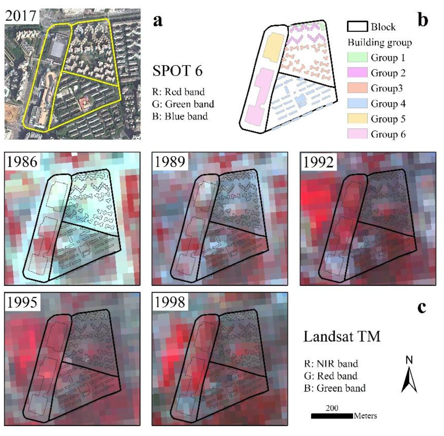
Figure 3.
Comparisons between the size of analysis units and the spatial resolution of Landsat imagery. (a) shows the contemporary buildings with different sizes in the street blocks, represented by the SPOT 6 imagery with a spatial resolution of 1.5 m. (b) shows the analysis units of street block, building group, and single building. (c) shows the differences between buildings with different sizes and Landsat imagery with the spatial resolution of 30 m, and changes within the analysis units.

Figure 4.
The temporal accuracies of building age estimation by using the four analysis units. The panels (a–d) represent the error matrixes for assessing the ability to identify the building age. The first column is the validation from year by year and the second one is from two-year tolerance verification, respectively. The size of the bubble indicates the number of samples.

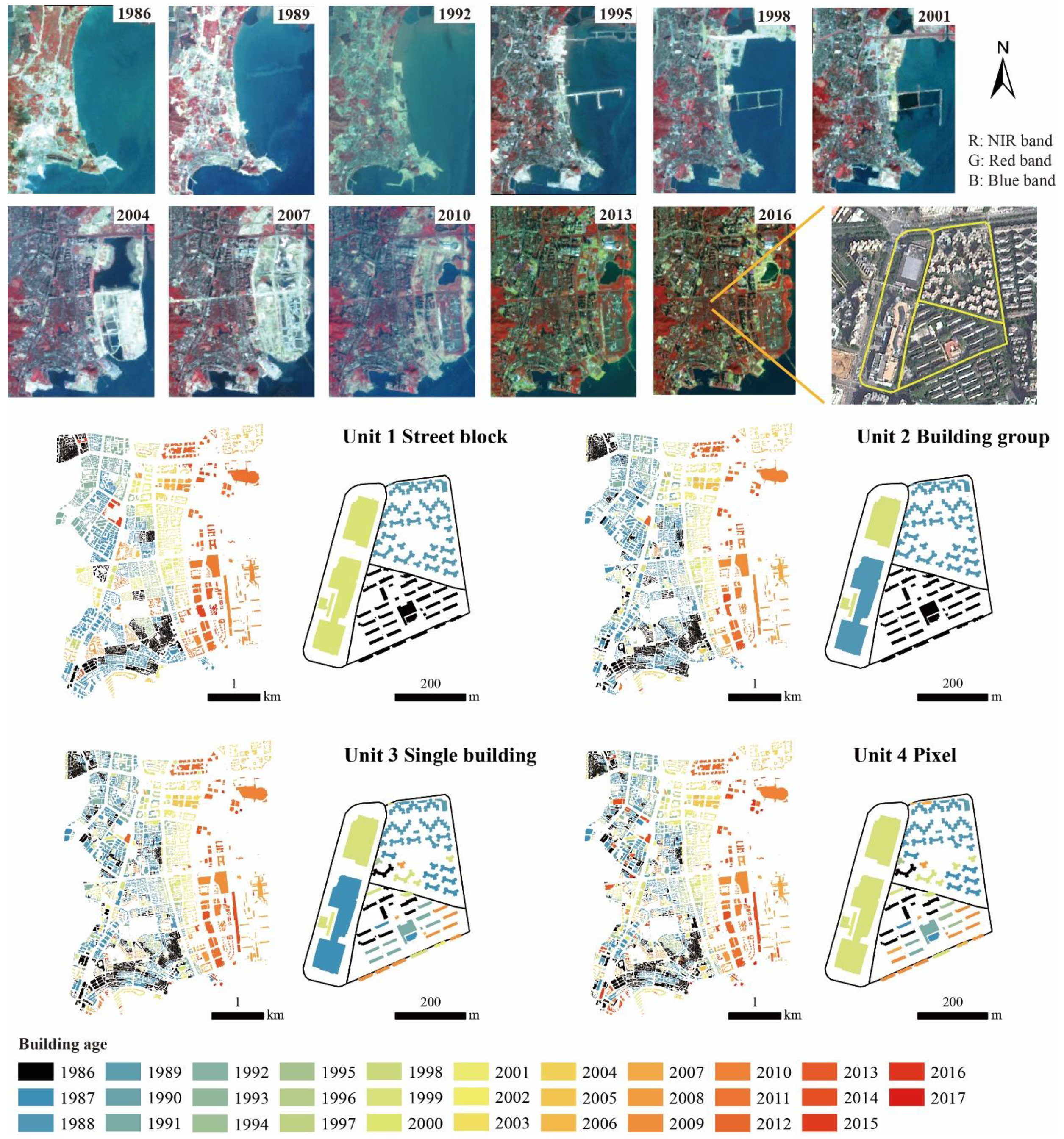
Figure 5.
The building age that estimated by the change detection with four units. The first two rows display the Landsat images from 1986 to 2016 and the subset display by the SPOT 6 in 2017. The last two rows are the building age estimated by using street block, building group, single building, and pixel.

Figure 6.
The spatial pattern of building age in Shenzhen during the period of 1986–2017. Panel (a) represents the spatial patterns of the older buildings and (b) shows that of the relatively new buildings.
Figure 6.
The spatial pattern of building age in Shenzhen during the period of 1986–2017. Panel (a) represents the spatial patterns of the older buildings and (b) shows that of the relatively new buildings.

Figure 7.
Building change in Shenzhen from 1986–2017. (a) is the building number and percentage of four levels; (b) is the building height of newly constructed ones and of all in one year.
Figure 7.
Building change in Shenzhen from 1986–2017. (a) is the building number and percentage of four levels; (b) is the building height of newly constructed ones and of all in one year.

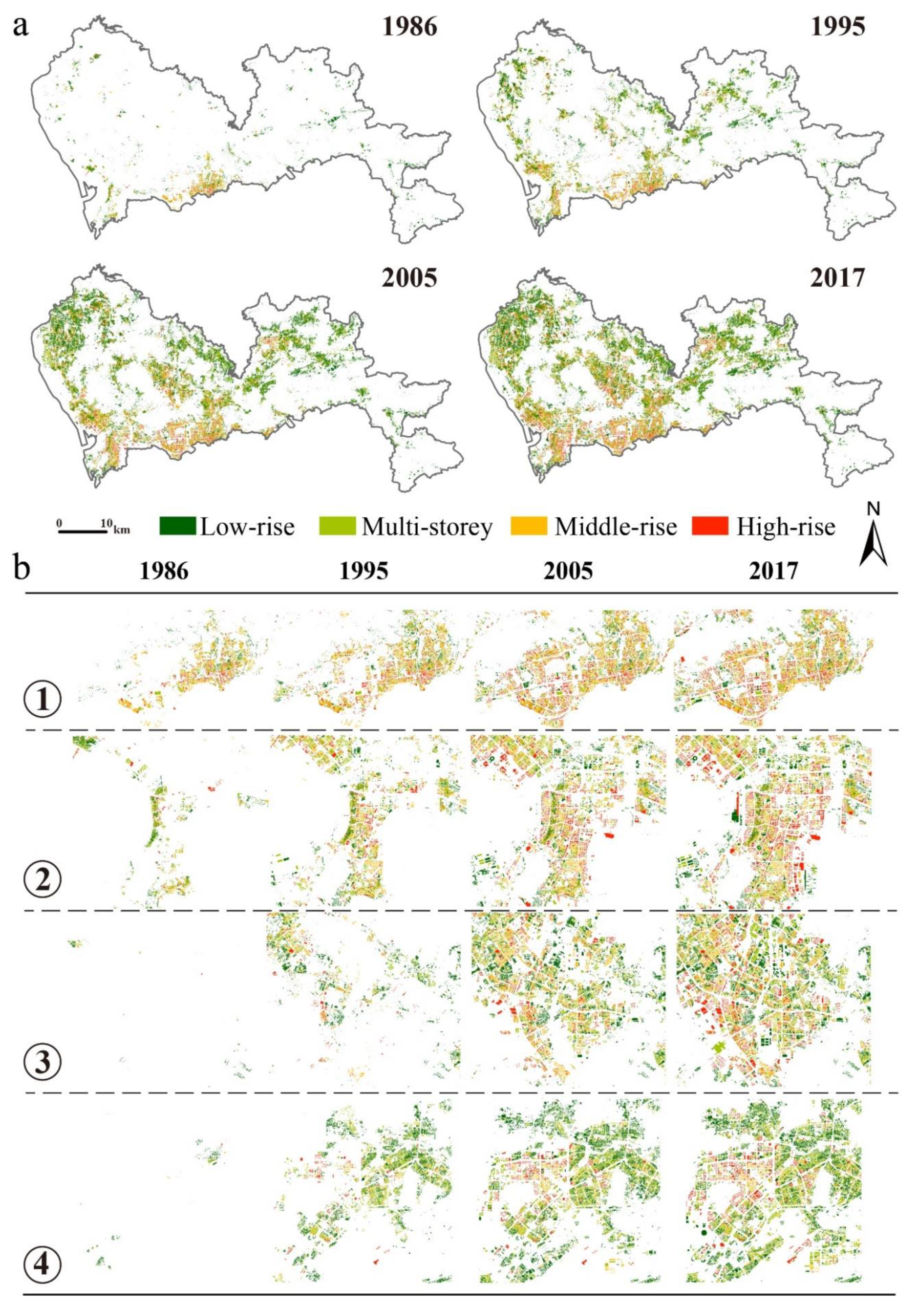
Figure 8.
The spatiotemporal patterns of urban 3D structure from 1986 to 2017. (a) shows the spatial patterns of buildings with different height levels and (b) shows the subsets of the four centers with high-rise buildings.
Figure 8.
The spatiotemporal patterns of urban 3D structure from 1986 to 2017. (a) shows the spatial patterns of buildings with different height levels and (b) shows the subsets of the four centers with high-rise buildings.


Table 1.
Error matrix for assessing the ability to distinguish the change from no-change categories.
Table 1.
Error matrix for assessing the ability to distinguish the change from no-change categories.
| Unit 1 Street Block | Reference | ||||
| No-Change | Change | Total | User’s Acc. (%) | ||
| Detected | No-change | 373 | 38 | 411 | 90.75 |
| Change | 98 | 491 | 589 | 83.36 | |
| Total | 471 | 529 | 1000 | ||
| Producer’s Acc. (%) | 79.19 | 92.82 | |||
| Overall Acc. (%) | 86.40 | ||||
| Unit 2 Building Group | Reference | ||||
| No-Change | Change | Total | User’s Acc. (%) | ||
| Detected | No-change | 401 | 52 | 453 | 88.52 |
| Change | 70 | 477 | 547 | 87.20 | |
| Total | 471 | 529 | 1000 | ||
| Producer’s Acc. (%) | 85.14 | 90.17 | |||
| Overall Acc. (%) | 87.80 | ||||
| Unit 3 Single Building | Reference | ||||
| No-Change | Change | Total | User’s Acc. (%) | ||
| Detected | No-change | 377 | 57 | 434 | 86.87 |
| Change | 94 | 472 | 566 | 83.39 | |
| Total | 471 | 529 | 1000 | ||
| Producer’s Acc. (%) | 80.04 | 89.22 | |||
| Overall Acc. (%) | 84.90 | ||||
| Unit4 Pixel | Reference | ||||
| No-change | Change | Total | User’s Acc. (%) | ||
| Detected | No-change | 364 | 52 | 416 | 87.50 |
| Change | 107 | 477 | 584 | 81.68 | |
| Total | 471 | 529 | 1000 | ||
| Producer’s Acc. (%) | 77.28 | 90.17 | |||
| Overall Acc. (%) | 84.10 | ||||
Note: Acc. represents accuracy.
Publisher’s Note: MDPI stays neutral with regard to jurisdictional claims in published maps and institutional affiliations. |
© 2021 by the authors. Licensee MDPI, Basel, Switzerland. This article is an open access article distributed under the terms and conditions of the Creative Commons Attribution (CC BY) license (https://creativecommons.org/licenses/by/4.0/).
Share and Cite
MDPI and ACS Style
Yu, W.; Jing, C.; Zhou, W.; Wang, W.; Zheng, Z. Time-Series Landsat Data for 3D Reconstruction of Urban History. Remote Sens. 2021, 13, 4339. https://0-doi-org.brum.beds.ac.uk/10.3390/rs13214339
AMA Style
Yu W, Jing C, Zhou W, Wang W, Zheng Z. Time-Series Landsat Data for 3D Reconstruction of Urban History. Remote Sensing. 2021; 13(21):4339. https://0-doi-org.brum.beds.ac.uk/10.3390/rs13214339
Chicago/Turabian StyleYu, Wenjuan, Chuanbao Jing, Weiqi Zhou, Weimin Wang, and Zhong Zheng. 2021. "Time-Series Landsat Data for 3D Reconstruction of Urban History" Remote Sensing 13, no. 21: 4339. https://0-doi-org.brum.beds.ac.uk/10.3390/rs13214339
Note that from the first issue of 2016, this journal uses article numbers instead of page numbers. See further details here.