
Zero-Shot Pipeline Detection for Sub-Bottom Profiler Data Based on Imaging Principles


1
School of Geodesy and Geomatics, Wuhan University, Wuhan 430079, China
2
Institute of Marine Science and Technology, Wuhan University, Wuhan 430079, China
*
Author to whom correspondence should be addressed.
Remote Sens. 2021, 13(21), 4401; https://0-doi-org.brum.beds.ac.uk/10.3390/rs13214401
Submission received: 22 September 2021
/
Revised: 28 October 2021
/
Accepted: 30 October 2021
/
Published: 1 November 2021
(This article belongs to the Special Issue Deep Learning for Radar and Sonar Image Processing)
Abstract
:With the increasing number of underwater pipeline investigation activities, the research on automatic pipeline detection is of great significance. At this stage, object detection algorithms based on Deep Learning (DL) are widely used due to their abilities to deal with various complex scenarios. However, DL algorithms require massive representative samples, which are difficult to obtain for pipeline detection with sub-bottom profiler (SBP) data. In this paper, a zero-shot pipeline detection method is proposed. First, an efficient sample synthesis method based on SBP imaging principles is proposed to generate samples. Then, the generated samples are used to train the YOLOv5s network and a pipeline detection strategy is developed to meet the real-time requirements. Finally, the trained model is tested with the measured data. In the experiment, the trained model achieved a [email protected] of 0.962, and the mean deviation of the predicted pipeline position is 0.23 pixels with a standard deviation of 1.94 pixels in the horizontal direction and 0.34 pixels with a standard deviation of 2.69 pixels in the vertical direction. In addition, the object detection speed also met the real-time requirements. The above results show that the proposed method has the potential to completely replace the manual interpretation and has very high application value.
1. Introduction
As the offshore oil and gas industry grows, more and more pipelines are being laid into the ocean [1]. On the one hand, the pipeline routes and buried depth should be surveyed in time and stored as historical data [2,3]. On the other hand, the condition of the pipeline needs to be checked periodically in order to prevent damage to the pipeline from fishing activities, turbulence, tidal abrasion or sediment instability [4,5,6,7]. Sub-bottom profiler, as a kind of specially designed sonar to explore the first layers of sediment below the seafloor (usually over a thickness that commonly reaches tens of meters) [8] (p. 372), can detect not only exposed and suspended pipelines but also buried pipelines, and is therefore widely used in underwater pipeline survey tasks.
Due to the working principle of SBP, pipeline measurements need to be performed along the direction perpendicular to the pipeline. In order to fully obtain the location information of the pipeline, repeated measurements are required at different positions of the pipeline. Therefore, it is crucial to identify the pipeline in the measured data in time so as to improve the measurement efficiency. In addition, unmanned measurement technology is gradually popularized, real-time and robust discovery of pipelines is also of great significance for surveying robots to plan routes autonomously [9,10,11,12].
Many researchers have studied the use of SBP for underwater pipeline detection [13,14,15,16], but the data processing still remains at the stage of manual interpretation, which is time-consuming and labor-intensive, and the detection results are easily affected by the mental state of the workers. A pipeline target presents a hyperbola shape in the SBP image. Therefore, the detection of a pipeline in the SBP image is similar to the detection of buried objects in ground penetrating radar (GPR) data. There is extensive literature about the detection of buried objects in GPR. Most of them are based on the curve fitting method [17,18,19,20,21,22,23], which has good enlightening significance for pipeline detection in SBP data. Traditional machine learning methods [24,25] are also used in the detection of hyperbola, but the performances are limited by the quality of samples. Recently, Li et al. proposed an efficient pipeline detection method based on edge extraction [26], which achieves a high correct detection rate, but computational efficiency is slow. Affected by a variety of imaging factors, the shape of pipeline in SBP images varies greatly, leading to difficulties in feature extraction, which makes it hard to detect the submarine pipelines automatically [27].
Recently, object detection methods based on DL have been widely used in various industries. Artificial neural networks, with their powerful feature learning capability, are able to extract significant information from complex data and achieve better performance than traditional methods [28,29,30]. Therefore, it is of great significance to introduce DL techniques to the automatic detection of pipelines. However, in order to obtain excellent trained models, DL methods require massive representative samples. The difficulty of acquiring sonar image samples limits the application of DL methods. In order to solve the problem, some researchers have studied the simulation of the samples for side-scan sonar (SSS) and achieved encouraging results [31,32,33,34], which is a good insight to solve the problem of lacking SBP pipeline samples. The working principle of SBP is different from that of side-scan sonar. Therefore, specialized sample synthesis methods need to be investigated. In addition, the SBP image usually has a large size, while the pipeline image has a simple structure and occupies a relatively small area of the image, which means that well-designed detection strategies are required to achieve fast and accurate detection of pipelines.
Given the problems of pipeline detection in SBP image, this paper proposes a real-time automatic pipeline detection method without using the measured samples. First, the imaging principle of SBP and the characteristics of pipeline in SBP image are introduced in detail. Next, based on the imaging principle, an efficient pipeline sample synthesis method is proposed to generate representative samples. Then, YOLOv5s are trained with the simulated samples. Finally, the measured data are used to test the effectiveness of the trained model. In addition, the performance of the proposed real-time pipeline detection method is also verified.
2. Materials and Methods
This section begins with a brief introduction of the working principle of sub-bottom profiler and the pipeline imaging mechanism is analyzed. Then, the sample synthesis method is introduced in detail. Finally, the real-time detection method of pipeline in sub-bottom images is presented.
2.1. Sub-Bottom Profiler Working Principle and Pipeline Imaging Mechanism
2.1.1. Sub-Bottom Profiler Working Principle
Technologically speaking, sub-bottom profilers are usually single-beam sounders working at high level and low frequency (1~10 kHz) [8] (p. 372). Some models are based on nonlinear acoustics and have a narrow beam in spite of small transducers and virtually no side lobes [27]. However, no matter what type of shallow profiler, their working principle is basically the same, they are all based on the specular reflection echo instead of a backscattered signal.
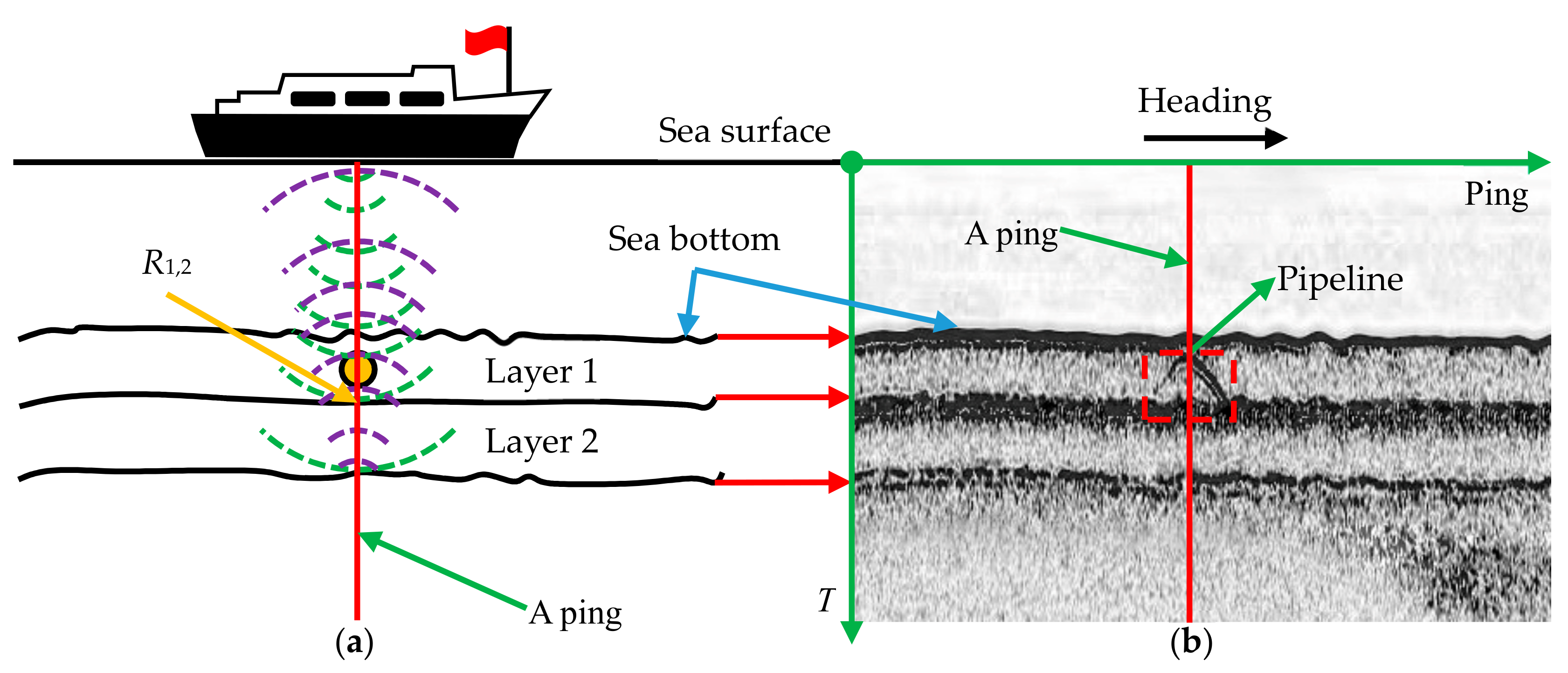
During the measurement, the transducer periodically emits acoustic pulses vertically downward toward the seafloor. The acoustic wave transmitted first propagates in the water column and the transducer only receives background noise or echoes from mid-water targets. When the acoustic pulse reaches the seafloor, some of the energy will bounce off the seafloor, while the remaining energy will penetrate the seafloor and continue to propagate [34]. When the acoustic impedance of adjacent strata changes greatly, the acoustic pulse will be strongly reflected, as shown in Figure 1a. The reflection coefficient R1,2 of adjacent layers can be calculated by:
where ρ is the density of sediments; c is propagation velocity of sound waves in sediments. When the intensity of the incident sound wave at the interfaces between layers is Aincident, the reflection intensity can be calculated by Equation (2).
The echo signals are recorded by the receiver and each acoustic pulse results in a sequence of echoes, also called a ping, reflecting any sort of density disturbance at the nadir of the sonar [35]. The successive echo sequences are arranged in order along the track to form a geophysical cross-section of the sediment layering, which will assist the user to visualize the morphology of the sedimentary layers and buried features.
2.1.2. Imaging Mechanism of Pipeline Target
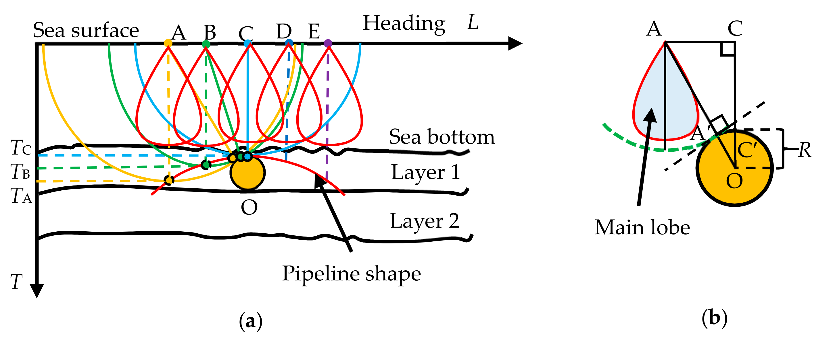
When the measurement is carried out along the direction perpendicular to the pipeline, a specular reflection signal will occur and be recorded, as long as the pipeline is within the effective range of the SBP. The reflection point is exactly the tangent point of the spherical surface and the pipeline, as shown in Figure 2.
Assuming that the propagation speed of sound waves is c (ignoring the variation of sound speed), the shape of the pipeline in the raw SBP waterfall image can be expressed as Equation (3):
where TC represents the Two-Way Travel Time (TWTT) for the sound wave to propagate from the sea surface directly above the pipeline to its upper edge; TA is the TWTT of the echo from the pipeline in each ping; R is the pipeline radius; xA and yA are the ping number and the sampling number, respectively, corresponding to the horizontal coordinate and vertical coordinate in the waterfall image; p is the ping rate (ping/s); v is the average ship speed (m/s); ΔT is the sampling interval. It can be seen that the size of the pipeline in the waterfall image is mainly related to the radius of the pipeline, the distance from the pipeline to the water surface, and the effective beam angle of the SBP.
Although the pipeline shape in the SBP image can be predicted by Equation (3), there are many factors that can affect the imaging of the pipeline target, resulting in a large discrepancy between the actual imaging results and the ideal results, making it difficult for automatic pipeline detection. Some of the main influencing factors can be summarized as follows:
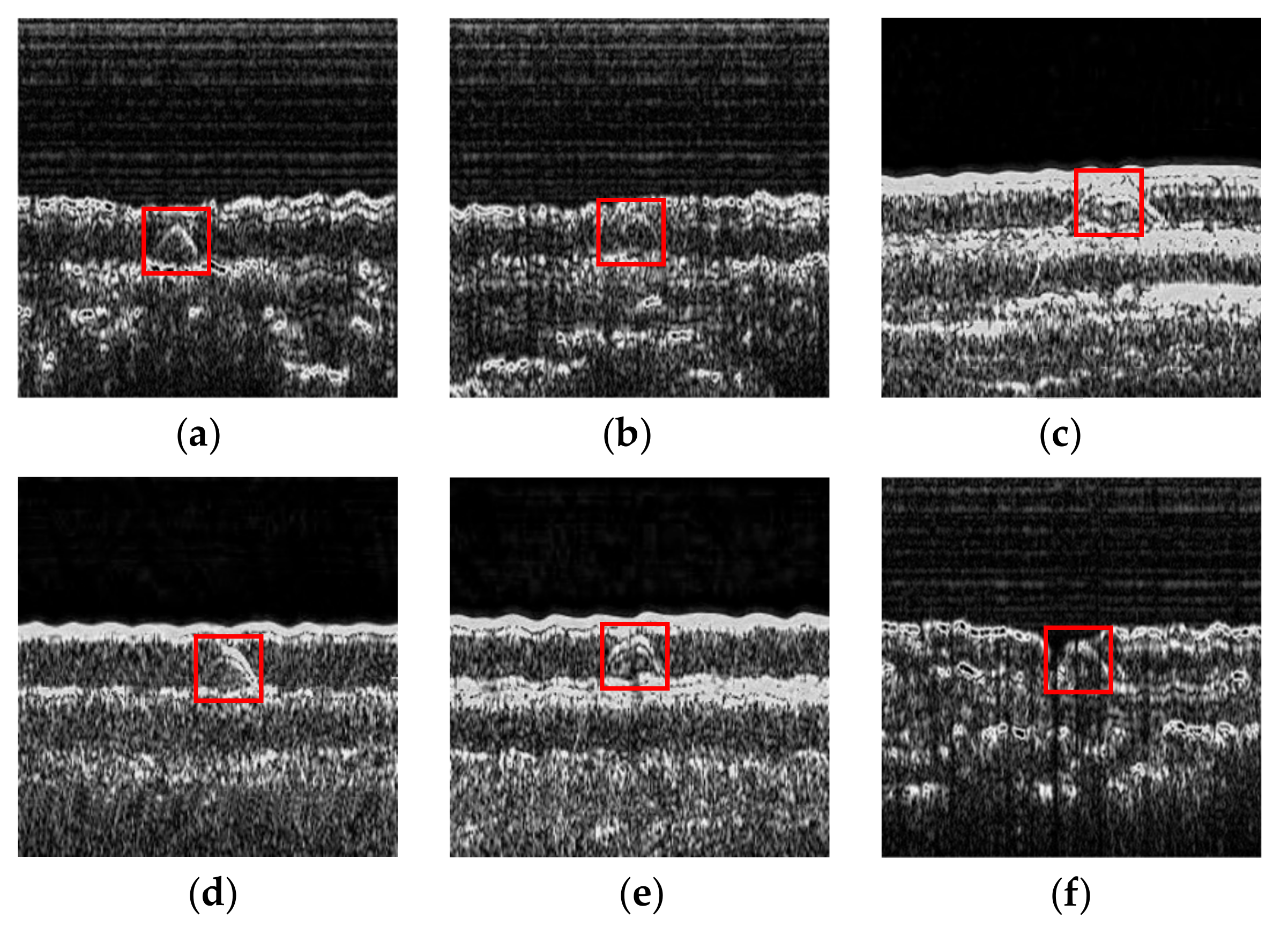
- High noise: The noise sources can be grouped into four categories, namely ambient noise, self-noise, reverberation and acoustic interference [8] (p. 123). The existence of noise greatly degrades the SBP image, resulting in low image contrast and blurred pipeline images. The images shown in Figure 3 are all disturbed by different degrees of noise.
- Small size: As described in Equation (3), if the pipeline is close to the water surface and the effective beam angle of the sonar is small, the size of the pipeline in the image will also be small, which is not conducive to distinguishing the pipeline from other reflectors, as shown in Figure 3a,b.
- Unfavorable position: The pipeline is usually buried at a lower depth in strata, when near the seafloor or layer boundaries, the echoes from the pipeline will be mixed with those from interfaces between media with different acoustic properties due to the limited vertical resolution of SBP, which makes it difficult to detect the pipeline automatically in the SBP image [27], as shown in Figure 3c.
- Small reflection coefficients: According to Equation (1), if the pipeline and the surrounding sediments have similar acoustic impedance, the reflection coefficients at the interface will be small. The echo from the pipeline at this time is weak and not easy to distinguish from the background, as shown in Figure 3d.
- Irregular movement: During the measurement, the survey ship will move up and down with the surge. If the SBP is fixed on the vessel, the distance from the equipment to the pipeline will also change accordingly, resulting in the deformation of the shape of the pipeline in the image. In addition, the uneven speed of the platform will also cause the pipeline imaging results to be compressed or stretched to varying degrees in the horizontal direction, as shown in Figure 3e.
- Missing pings: When there are a large number of bubbles around the sonar in the water, the mechanical vibrations generated by the transducer cannot be transmitted to the water in the form of acoustic pulses. As a result, the SBP cannot receive the effective echo signal, resulting in missing image information, as shown in Figure 3f.
2.2. General Data Pre-Processing Method
2.2.1. Quantization of Raw SBP Data
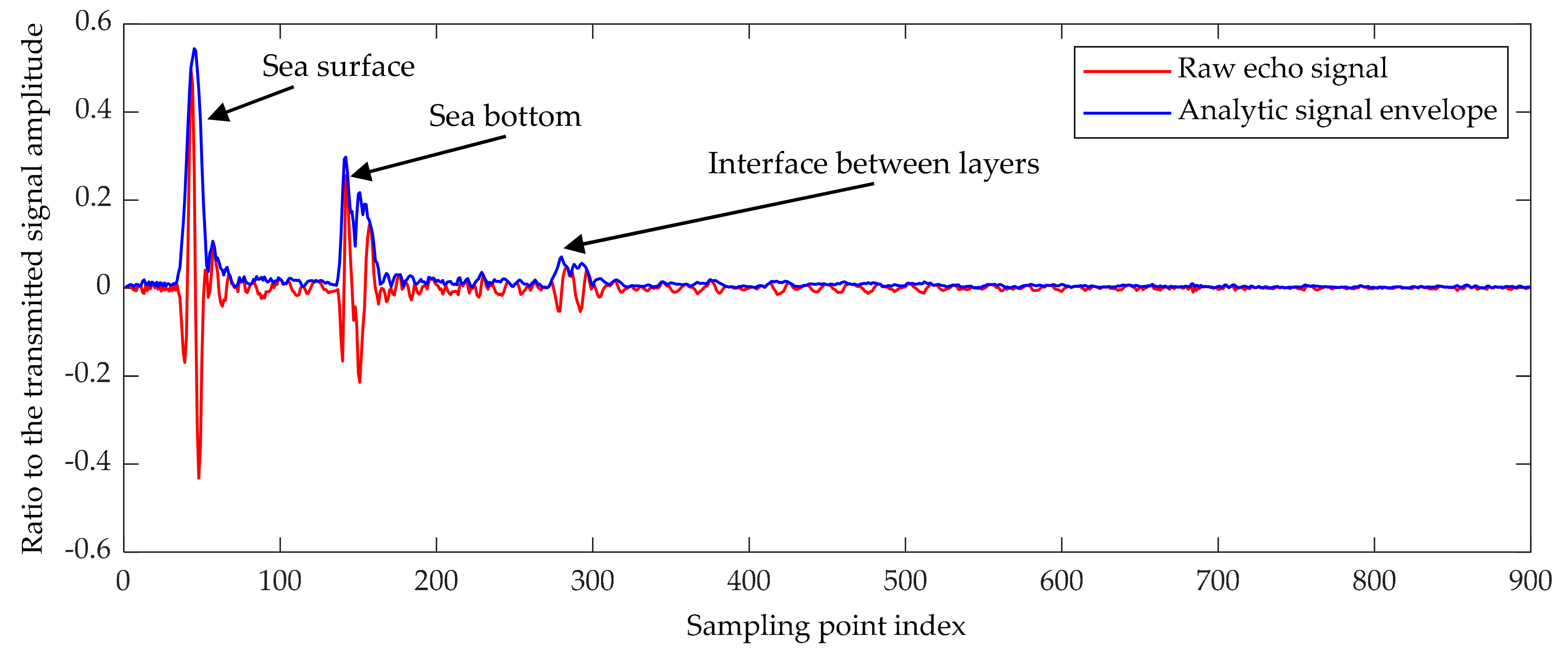
The raw echo data recorded by SBP are usually the ratio of the instantaneous sampling value of the echo signal to the amplitude of the emitted sound wave, as shown in Figure 4. In order to convert the raw echo data into grayscale values of pixels in the waterfall image, the instantaneous amplitude of the recorded echo sequence needs to be extracted first. For an echo signal sequence X(t), its Hilbert transform Y(t) can be expressed as Equation (6):
Thereby, the analytic signal of X(t) can be expressed as:
and finally, the envelope A(t) of the analytic signal g(t) is obtained by:
Then, the gray value of each sampling point is obtained by mapping the instantaneous amplitude of the sampling point to 0~255. The mapping process can be represented by Equation (9).
where As denotes the instantaneous amplitude of the sampling point, and Amin and Amax are the maximum and minimum amplitudes in each ping, respectively. Each ping of the raw echo data is processed as described above and arranged in order to form the raw SBP waterfall image.
2.2.2. Unification of Image Resolution
For the raw SBP waterfall image, the vertical resolution rv is related to the sampling period Ts of the sonar as well as the sound velocity c, as expressed by:
The sampling interval of the device is usually unchanged, while the propagation speed of sound waves in the medium is varying (typically, 1400 m/s~1600 m/s in water [36] and 1500 m/s~1800 m/s in shallow strata [37]). Therefore, the vertical resolution of raw SBP waterfall image is not a constant.
Similarly, the horizontal resolution rh is related to the ship speed v and the acoustic pulse emission period Tp, as expressed in Equation (11). Usually, the ship speed is not constant, therefore, the actual distance between adjacent pings is also constantly changing.
The inconsistent horizontal and vertical resolutions of the raw SBP waterfall map and their respective non-constancy will not only cause the deformation of the pipeline, but also lead to some layer boundaries with very similar shapes to the pipeline, causing interference to the pipeline detection.
To unify the vertical resolution, the sound velocity along the propagation path needs to be known, which is unrealistic in most cases. In order to simplify the calculation process and to keep the target deformation caused by inaccurate sound velocity within a reasonable range, an average sound velocity of 1600 m/s is used uniformly in this paper.
Generally, the vertical average resolution is higher than the horizontal one. In order to retain more target information after unifying the resolution, the average vertical resolution remains unchanged, and the raw waterfall image is interpolated horizontally, as shown in Figure 5.
For higher computational efficiency, the linear interpolation method is used in this paper. The pixel value Ii,j between adjacent pings can be calculated by:
where Lj = j × rv, denotes the actual distance of the j-th column of the interpolated image relative to the first column of the image, and Ln denotes the distance of the n-th ping of data relative to the first ping of data along the trajectory direction. Wi,n denotes the grayscale value of the i-th sampling point in the n-th column of the raw waterfall image. The result of a raw waterfall image after interpolation is shown in Figure 6.
2.3. An Efficient Sample Synthesis Method Based on SBP Imaging Principles
For data-driven object detection methods, it is very important for improving the correct detection rate to establish a dataset containing samples under various conditions. In reality, sufficient object samples are difficult to obtain, but we can easily obtain a large number of SBP data that do not contain pipeline targets. Although these data alone are not enough to build the pipeline detection model, they contain rich stratigraphic distribution information and can provide diverse backgrounds. In view of this, we propose an efficient method to generate representative pipeline samples by using the measured data without pipeline targets, which fully considers the imaging mechanism of the pipeline and various influencing factors while preserving the real measurement environment. The basic process is shown schematically in the Figure 7.
The raw data are firstly pre-processed to obtain the SBP image. Secondly, through the noise separation step, the noise image and the filtered image are obtained. Then, the filtered image is used to generate the pipeline image according to the imaging mechanism of the pipeline and considering the influencing factors during the measurement. Next, the pipeline image and the filtered image are merged to generate a synthetic image. Finally, the noise is added to the synthetic image to obtain the final synthetic sample. The specific methods in the key steps are described separately below.
- Noise Separation
There is a lot of noise in the image I obtained from the raw SBP data. These noises are caused by the real measurement environment and equipment themselves, therefore, they are important features of the image and it is extremely necessary to retain them during the sample synthesis process. The noises n act as external additions perturbing the expected signals [8] (p. 123), as expressed in Equation (13):
At present, there are many excellent de-noising algorithms. Among them, the non-local low-rank algorithm proposed in the literature [38] achieved excellent performance by taking advantage of the inherent layering structures of the SBP image and is therefore used for noise separation of SBP image in this paper. A more detailed description of this method can be found in the original text.
As shown in Figure 8, the noises are well separated by the de-noising algorithm. The noise image is saved for adding to the synthetic image in the final stage of sample synthesis, while the de-noised image is further used for generating the synthesized image.
- Pipeline Image Generation Based on Imaging Mechanism
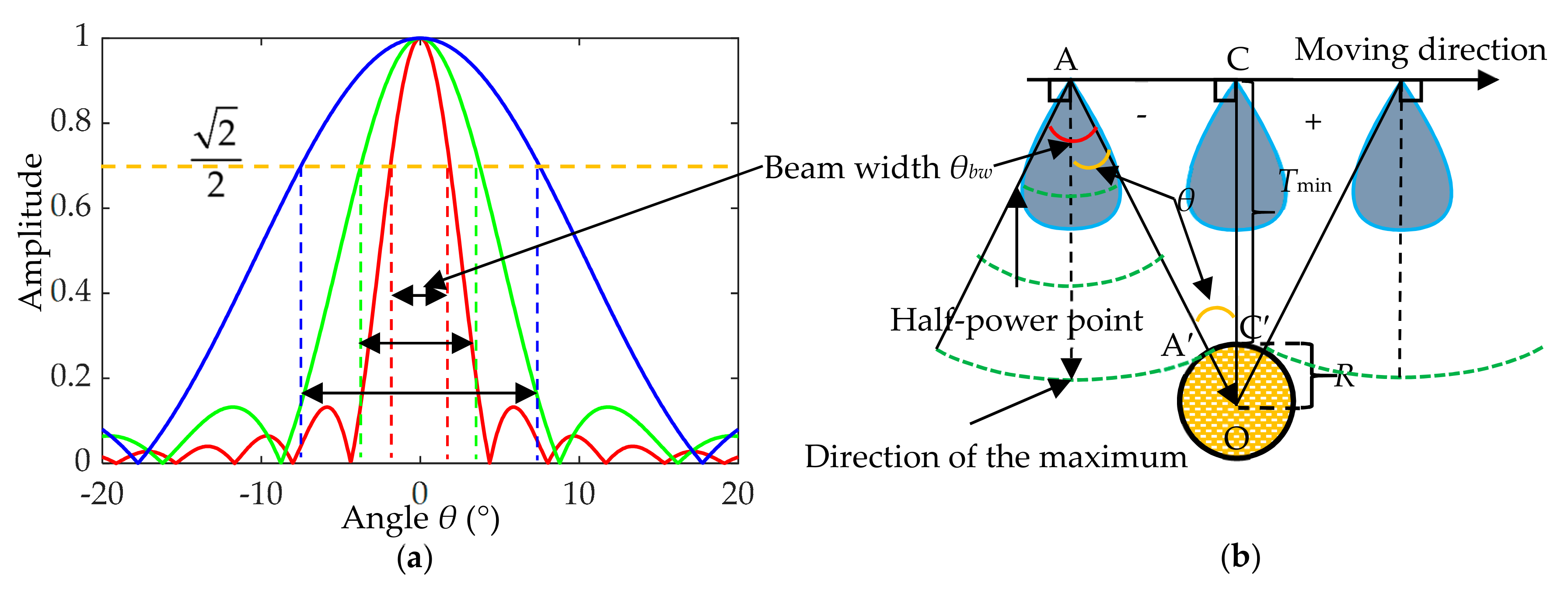
Transducer directivity is an important property of SBP, indicating the angular distribution of the acoustic energy radiated into the propagation medium in transmission and the electric response as a function of the arriving direction of the acoustic wave in reception. For a circular piston transducer with a diameter D, the far-field directivity can be calculated using the Bessel function of the first kind J1(x):
where λ denotes the acoustic wavelength. As shown in Figure 9a, there is usually a main lobe surrounded by a series of side lobes. The beam width θbw is corresponding to the angle between −3 dB on each side of the main lobe’s maximum. For a given transducer, the higher the frequency, the narrower the width of the beam.
When the carrier platform passes above the pipeline, the angle θ between the direction of the pipeline relative to the transducer and the direction of the maximum of the directivity pattern changes from −θbw/2 to +θbw/2, assuming that the angle value is negative when the transducer is on the left side of the line and positive on the other side, as shown in Figure 9b. The amplitude variation of the sound pulse hitting the pipeline can be exactly expressed by the directivity function Γ(θ). If the echo signal is also received by the same directivity pattern, assuming that the position change of the transducer during transmission and reception is negligible, the variation of the echo intensity from the pipeline caused by the directivity pattern can be expressed as:
As acoustic waves propagate in the medium, there are geometric spreading losses and absorption losses. When the pipeline is at the nadir of the transducer (θ = 0), the propagation distance is the shortest, therefore, the energy loss is the smallest. Taking the amplitude of the pipeline echo at this time as a reference, the relative values of the pipeline echo amplitude at different θ can be expressed as [8] (p. 23):
where Dmin is the minimum distance between the transducer and the pipeline; γ is the attenuation; Dθ is the sound propagation distance at different θ, and can be expressed as:
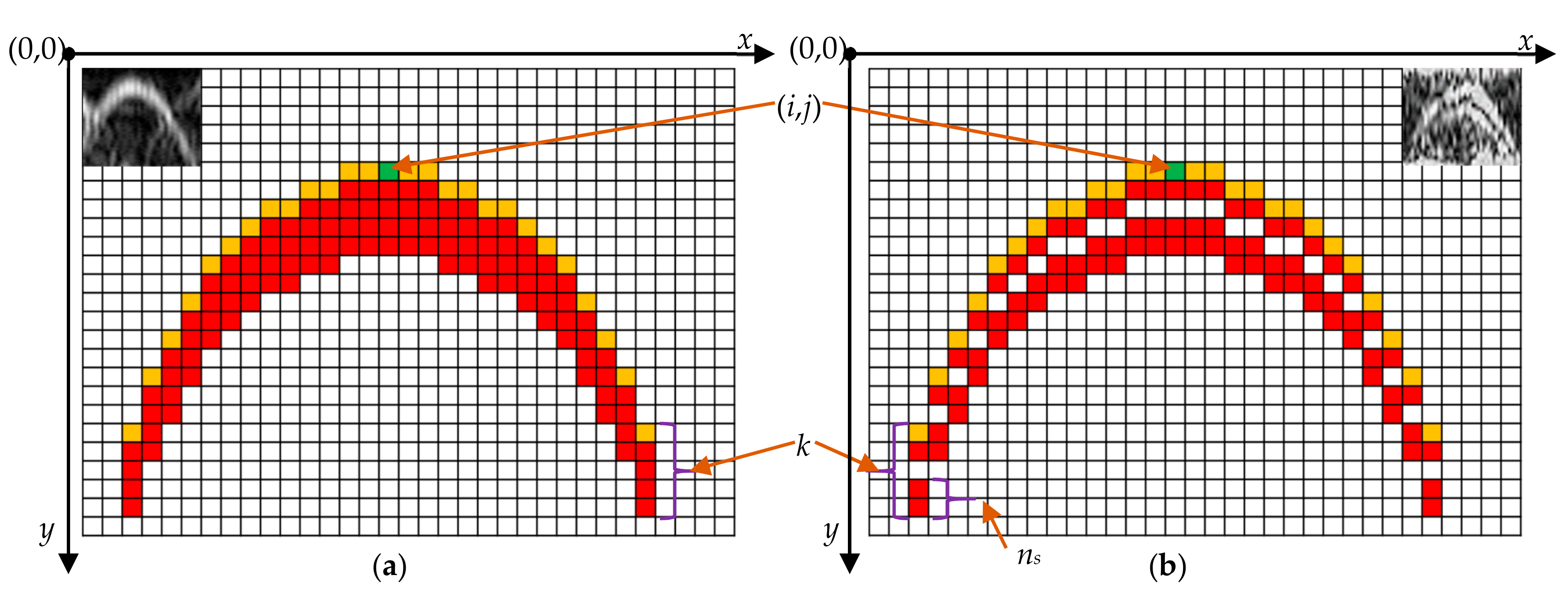
We have introduced the imaging mechanism of the pipeline in Section 2.1.2. The shape of the pipeline in the raw waterfall image can be described by Equation (3). While in the pre-processed SBP image, the shape Sp composed of the echoes from the upper edge of the pipeline (marked in yellow as shown in Figure 10) is expressed as:
where (i, j) is the coordinates of the highest point of the pipeline; (xp, yp) is the image coordinate of the pipeline shape, r is the unified image resolution and equal to the average vertical resolution rv.
The measurement resolution of a SBP is its ability to distinguish the echoes from two close distinct targets, which also has a significant impact on the appearance of the pipeline image. The range resolution can be calculated by:
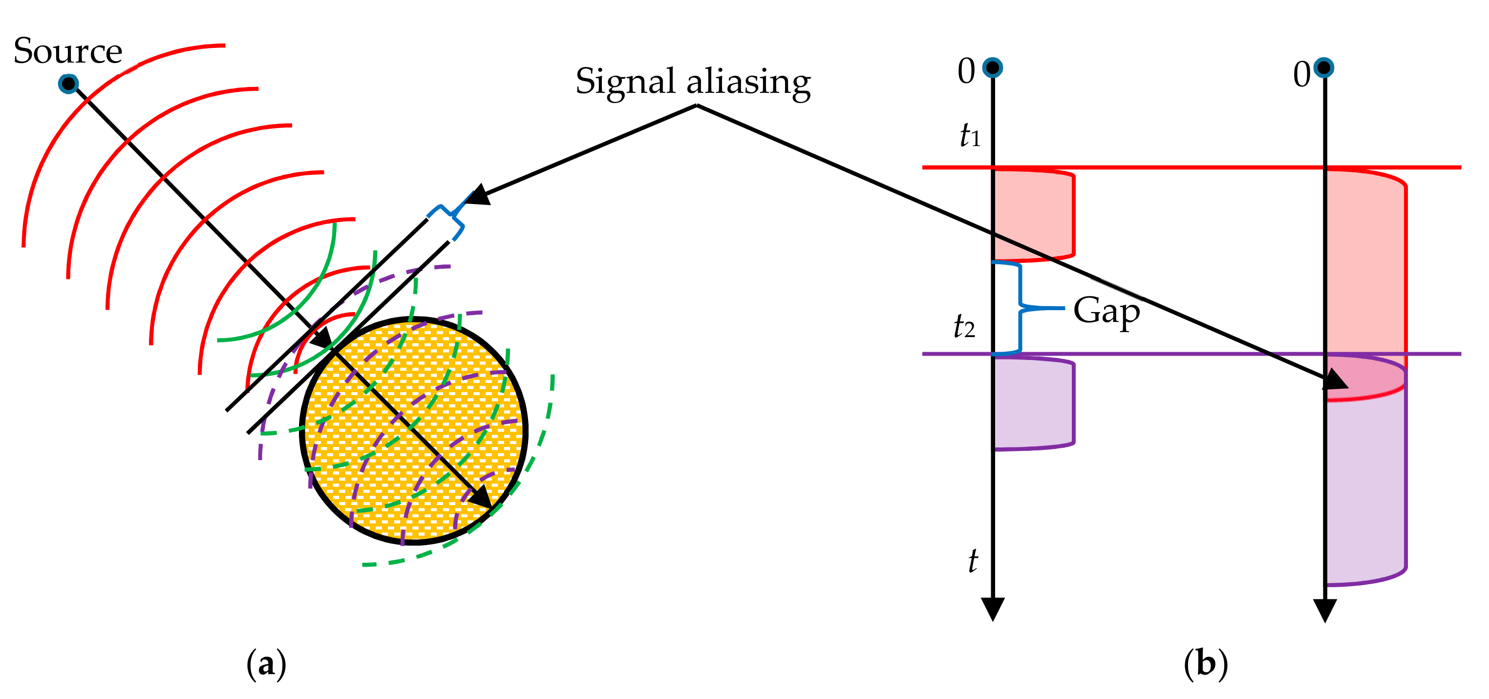
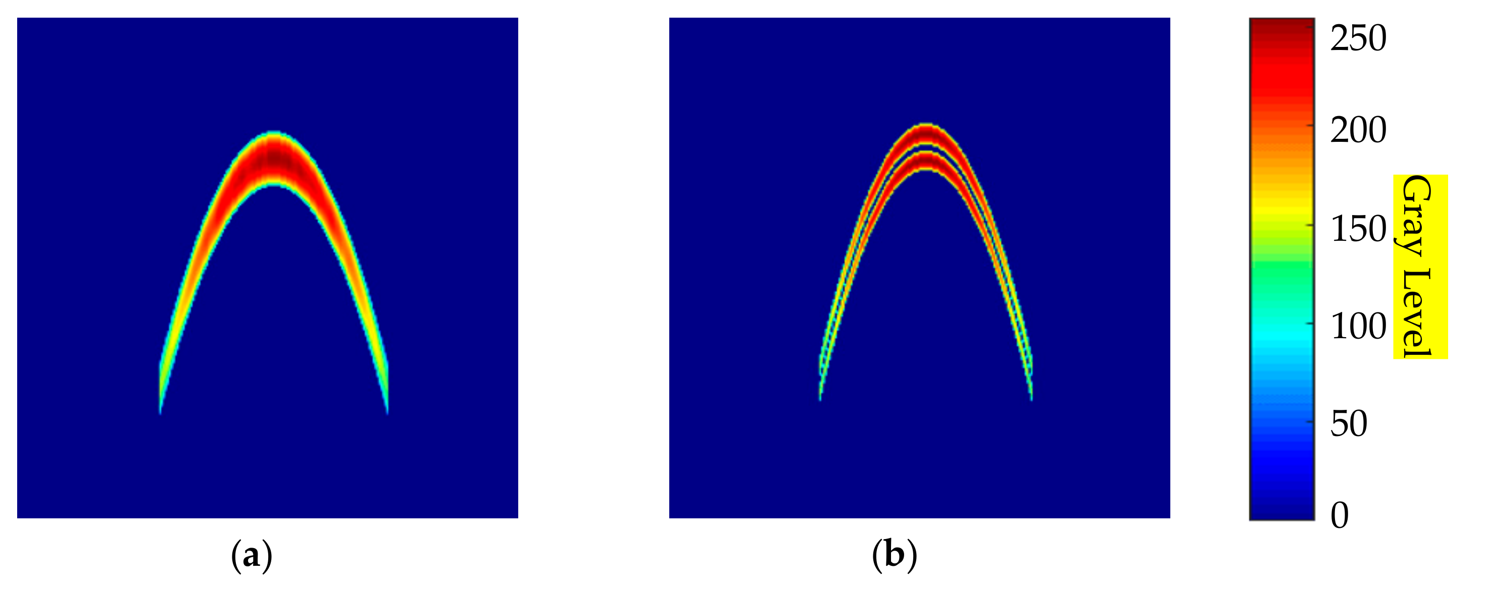
where c is the sound velocity, and Te is the effective pulse duration due to transmitter pulse length, directivity and bottom reverberation. When the diameter of the pipeline is smaller than the resolution of the SBP, the echoes from the upper surface of the pipeline will be mixed with the echoes from the lower surface, as shown in Figure 11, and the imaging results will be similar to Figure 10a. Otherwise, as seen in Figure 10a,b, there is a gap between the echoes from different surfaces.
The sampling interval of the transducer is generally much smaller than the length of the acoustic pulse it emits, so the echo signal from the pipeline will produce multiple pixels in a column of the image. The pixel number ns can be calculated by:
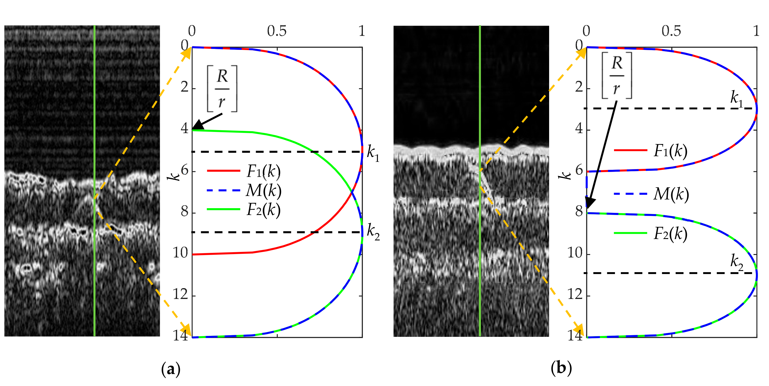
The actual measured pipeline echo signal is ridged in each ping, the main reasons for this phenomenon are the transient effect of the acoustic signal, scattering echoes, etc. For simplicity, we use the exponential form of a sinusoidal function to describe the ridge:
where k is pixel index relative to the first pipeline echo in each column of the image, ∈ [0, ns]; β is used to control the steepness of the function edge. For pipelines with different diameters, we uniformly use function Υ(k) to describe the changes in echo amplitude, as shown in Figure 12. Assuming that F1(k) and F2(k) correspond to the arrival period of echoes from different interfaces, when their intersection point value is greater than 0.5, the value of Υ(x) in the [k1, k2] segment is 1, otherwise the larger values of F1(k) and F2(k) are taken as the value of M(x) in [k1, k2].
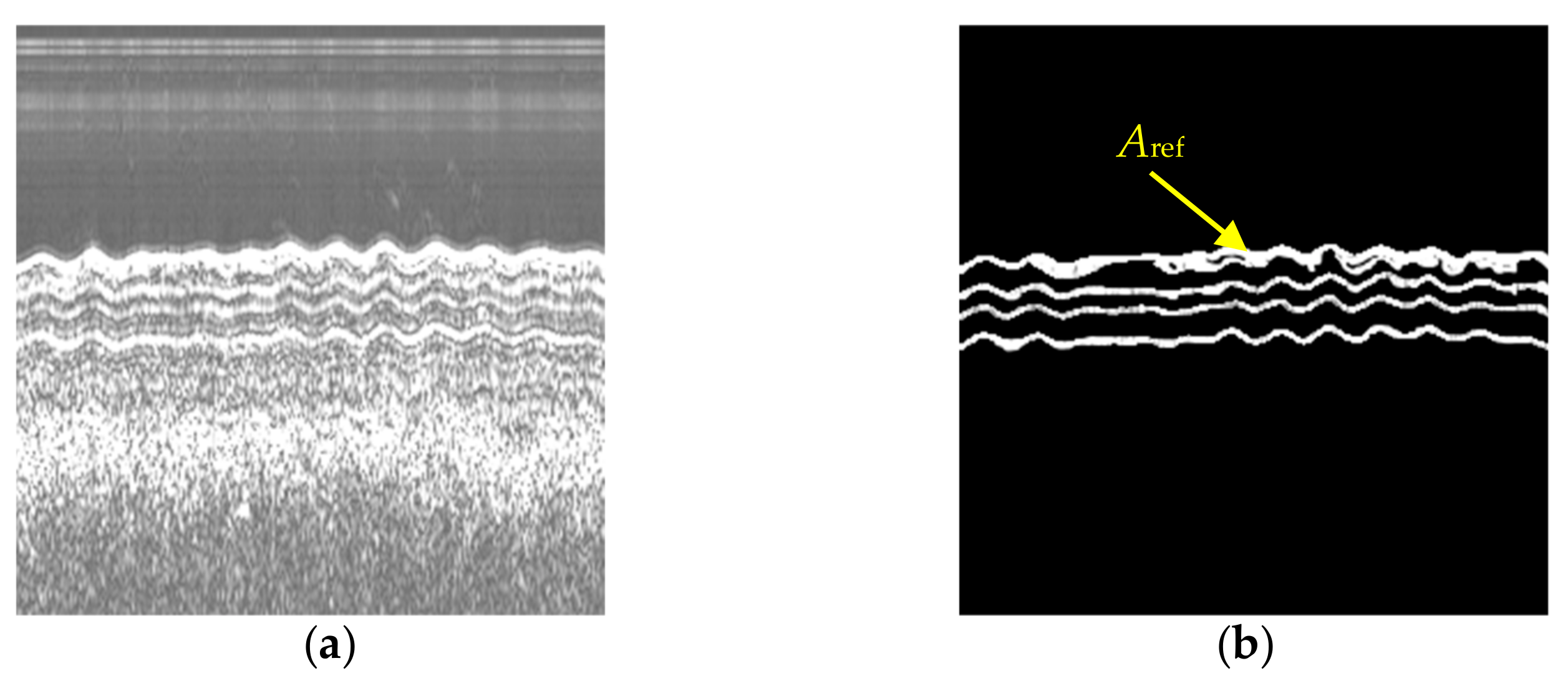
Most of the SBP data are measured by un-calibrated equipment, thus, the reflection coefficients as well as absorption coefficients associated with the sediment layers cannot be retrieved from these data [8] (p. 373), and accordingly, the echo intensity of pipelines with different burial depths cannot be accurately estimated either. In addition, the gain information of some SBP data is not recorded during the field measurement, resulting in uncorrectable radiometric distortions in the images. In summary, the echo intensity of pipelines is variable in different SBP images. Therefore, we can randomly select the amplitude of the echoes from the horizons in the SBP image as the reference value Aref, as shown in Figure 13, while the echoes from horizons in the SBP image can be easily extracted by manual or automatic methods proposed in the literature [39,40].
At this point, we can obtain the complete expression of the pipeline target in the SBP image under ideal conditions.
By changing the variables in the above equation, different pipeline images can be obtained. Figure 14 shows two generated pipeline images.
- Image Modification by Influencing Factors
- (1).
- Heave of carrier platform
The heave of the carrier platform will cause a change in the propagation distance of acoustic waves in the water, and since each column of the SBP image is aligned according to the propagation distance, the presence of carrier platform heave will lead to longitudinal deformation of the target in the image. Therefore, the heave of the carrier platform is considered as an influencing factor in sample synthesis, and it can be simulated by superimposing multiple sine waves:
where l is the number of sine waves, usually a value of 2 is sufficient. Ai, ωi, and φi are the amplitude, angular velocity and phase of the i-th sine wave, respectively.
- (2).
- Missing effective pipeline echoes
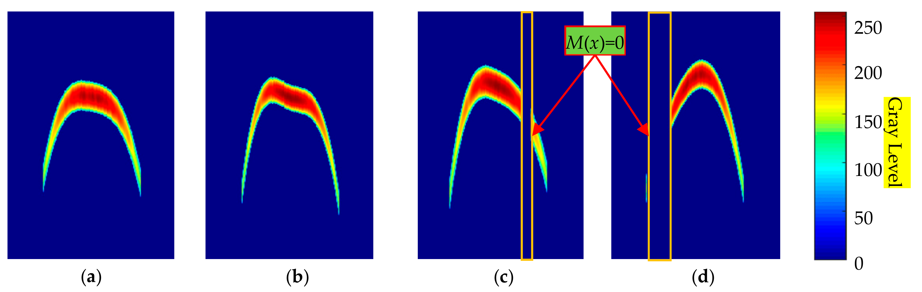
There may be no effective pipeline echoes in successive columns of the SBP image, which is due to the similarity of the acoustic impedance of the pipeline to its surrounding sediments, or the presence of missing pings during the measurement. We use a mask function to indicate whether a column of the pipeline image has valid echoes or not.
When the x-th column contains effective pipeline echoes, the function value is 1, otherwise it is 0. After adding the above two influencing factors to the imaging formula, we finally obtain the complete expression of the pipeline in the image:
Some generated pipeline images applied with the above influencing factors are shown in Figure 15.
- Merge
After obtaining the pipeline image, the next step is to fuse it with the filtered image from the noise separation step. To increase the representativeness of the samples, the position of the pipelines can be randomly selected with reference to the interfaces between layers, so as to simulate pipelines with different deployment states. Usually, the weaker echoes will be submerged in the stronger echoes. Therefore, the following formula is used for fusion:
Then, the noise is superimposed on the synthesized sample again, that is,
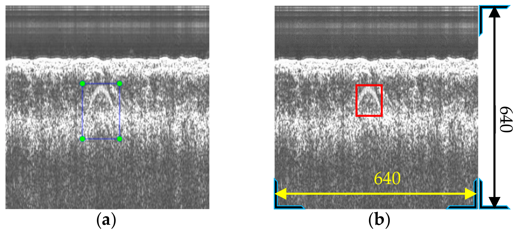
Finally, we obtain an image containing the pipeline target, and at the same time, the size and position of the target’s bounding box can be obtained, as shown in Figure 16a. However, due to the variable background, the actual distinguishable bounding box of the target can vary greatly in the synthesized sample. Therefore, skilled operators are required to optimize the labeling of the sample and eliminate unreasonable samples, as shown in Figure 16b. In this way, the operator’s experience is embedded in the samples. Thus, the network can also learn from human experience when trained with these samples.
2.4. Real-Time Pipeline Detection
2.4.1. Building Pipeline Detection Model
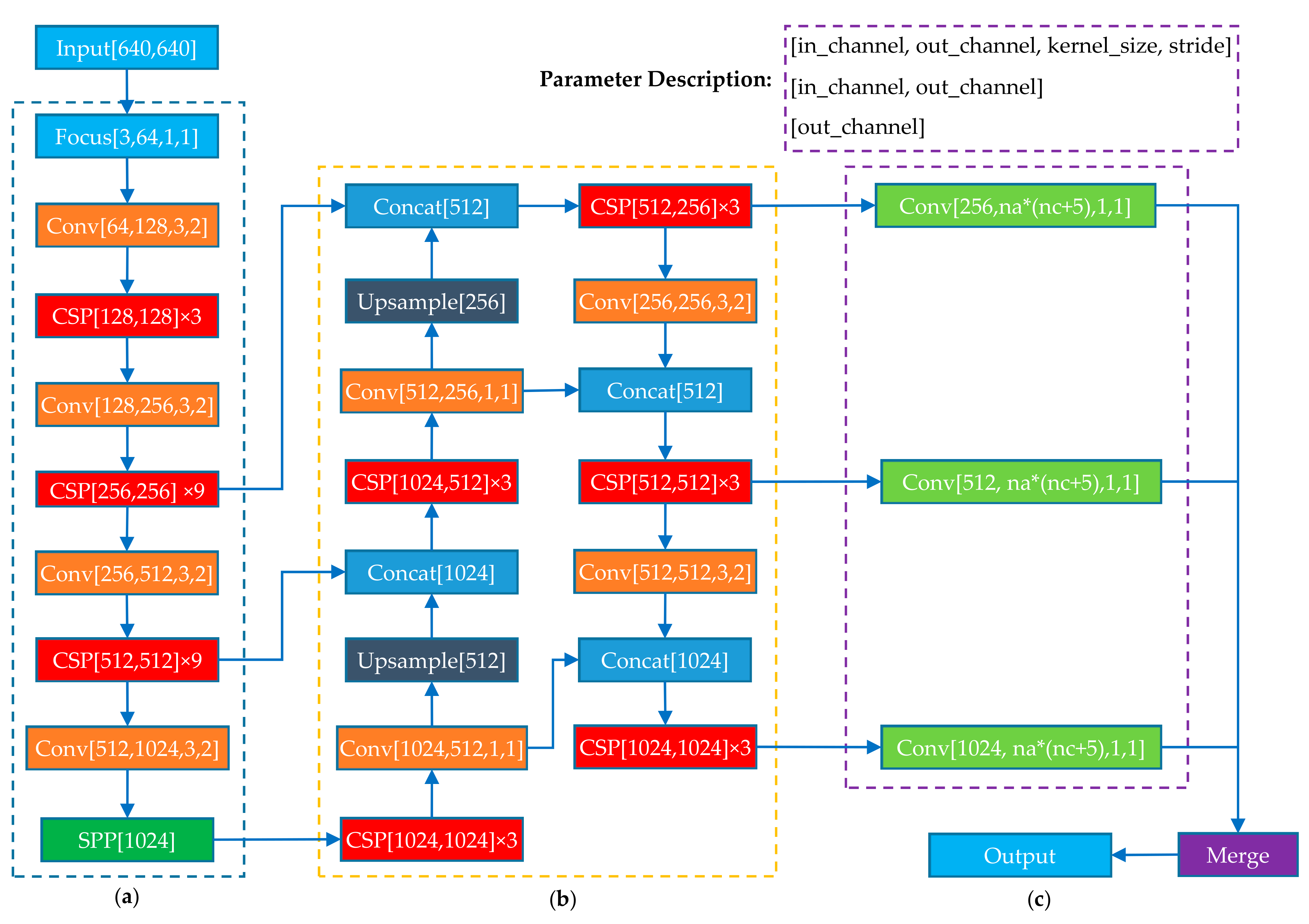
At this stage, many target detection network architectures have been proposed, such as R-CNN [41], SSD [42], Faster-RCNN [43] and YOYO series [44], and their powerful performance has been proven on various public datasets. Among them, YOLOv5, as the latest architecture of the YOLO series, not only has fast detection speed, but also high accuracy, and is widely used in real-time object detection. Considering the timeliness, this paper uses the YOLOv5s to construct the pipeline detection model. The basic structure of YOLOv5s is shown in Figure 17.
The network structure of YOLOv5s consists of three parts: backbone, neck and head. The backbone, CSPDarknet [45], can effectively extract feature information from the input image through multiple down-sampling. The neck is responsible for aggregating the image features extracted by the backbone with the cascade structure of FPN and bottom-up PANET. The head contains three output branches, which predict the bounding boxes and categories of objects of different sizes. The input image is divided into an S × S grid. For each grid cell, YOLOv5s predicts B bounding boxes. Each bounding box includes 3 categories of parameters, they are the position (x, y, w, h) corresponding to (center coordinate (x, y), width, height) of a bounding box, object confidence C and prediction probabilities P of N classes. Therefore, the loss function is composed of bounding box position loss, object confidence loss and class probability loss, as expressed in Equation (28). The bounding box position loss adopted here is the GIOU loss proposed in the literature [46]. The object confidence loss and class probability loss are calculated by the cross-entropy loss function.
where is defined as 1 if object presents inside j-th predicted bounding box in i-th cell, and 0 for otherwise. is the opposite. λcoord and λnoobj are the loss weights.
For the application in this paper, there is only one class of object. The network is trained end-to-end with the synthesized samples. When the accuracy of the trained model is not increasing, it is saved for the detection of measured data.
2.4.2. Real-Time Pipeline Detection Strategy
In the real-time pipeline detection scenario, whenever new ping data arrive, the newly added data need to be detected once, and the detection process needs to be completed before the next ping data arrive. The specific steps are as follows:
- Data pre-processing. First, the ship speed is estimated based on the already measured navigation data. Then, according to the time difference Δt between the new ping and the previous ping, the distance between adjacent pings can be calculated, and finally, the ping is quantified with the method described in Section 2.2.1 and the image between this ping and the previous ping is interpolated using the method introduced in Section 2.2.2.
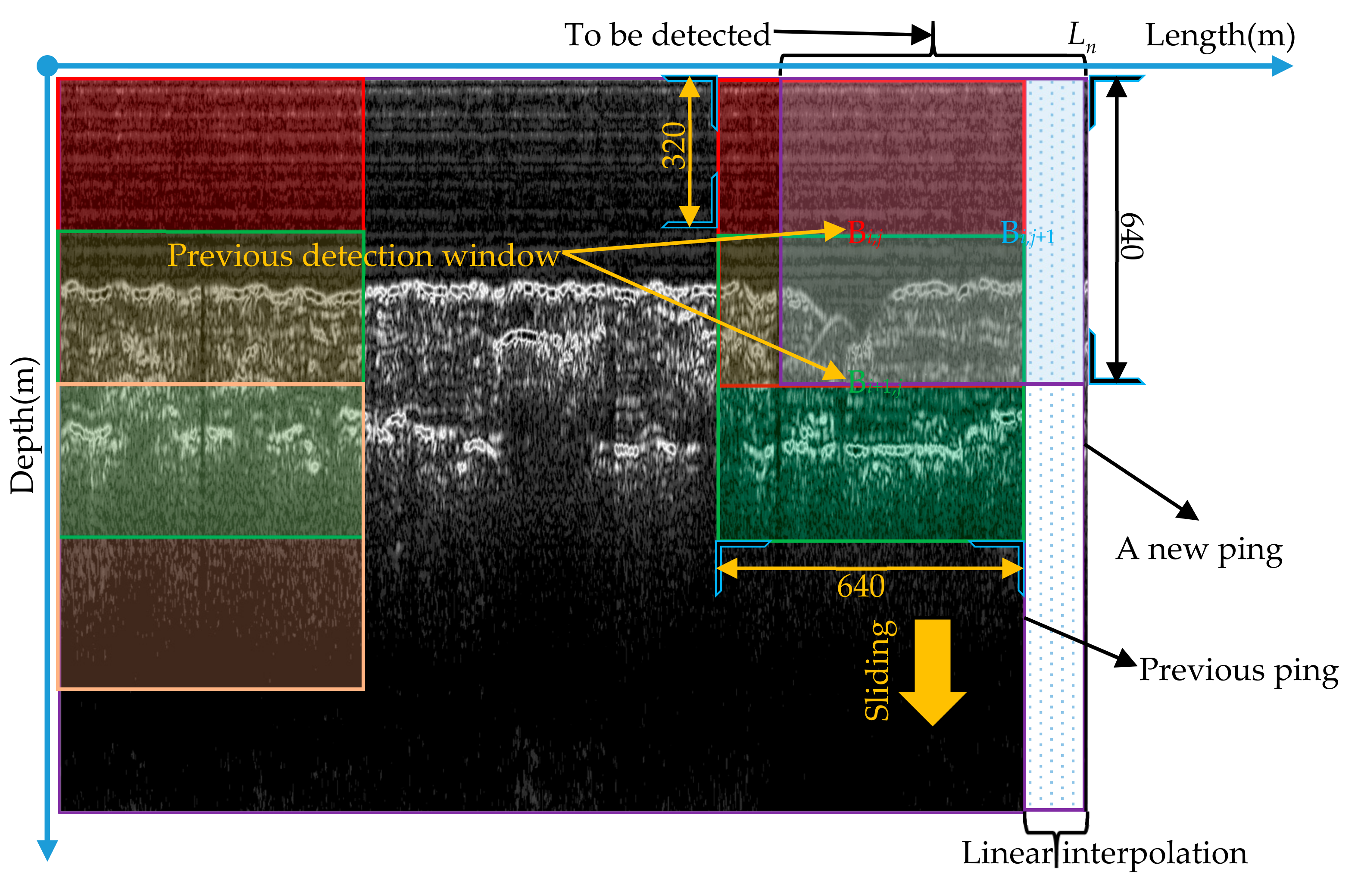
- Sliding window detection. For the newly-added image part, pipeline detection is performed with a sliding window of 640 × 640 using the detection model constructed in Section 2.4.1, and adjacent windows have a 50% overlap, as shown in Figure 18.
- Bounding box fusion. Since any two adjacent detection windows have different degrees of overlap, the same target may be detected multiple times. In addition, the detection is performed using a sliding window; therefore, it can happen that only part of the target is inside the window, and the detected bounding box is incomplete at that time. In order to ensure the uniqueness and completeness of the detection results for the same target, it is necessary to fuse the detected bounding boxes of the same target in different detection windows. Whether it is the same target can be determined by Equation (29).where Bi and Bj are the bounding boxes detected in the adjacent windows Wi and Wj. Woverlap is the overlap of the adjacent windows, equal to Wi ∩ Wj. If IoUoverlap > 0.8, the targets in Bi and Bj are judged to be the same target, and the union of Bi and Bj is taken as the new bounding box of the target. By judging all detection windows with overlapping parts, the fusion of the same target bounding box is realized.
3. Experiments and Results
To verify the effectiveness of the proposed method, the raw SBP data collected by C-Boom in Jiaozhou Bay, EdgeTech 3100P in Zhujiang Estuary and Parasound P70 in South China Sea, in which there are no pipe targets, are selected for sample synthesis, and the pipeline investigation data collected by Chirp III in Yangtze Estuary and Edgetech 3200XS in Bohai Bay are used to test the performance of the trained model. All the data were recorded in the SEG-Y data format, and they were pre-processed with the method presented in Section 2.2. The test data were disturbed by the influencing factors described in Section 2.1.2, which are highly representative and cover most complex situations.
3.1. Sample Synthesis
The proposed sample synthesis method involves numerous variables, and some reasonable value ranges are listed in Table 1, depending on the actual circumstances that may be encountered during the measurement.
For the diversity of samples, all the involved values are randomly selected from these intervals for sample synthesis, and the influences of carrier platform heave and missing effective pipeline echoes are applied to the generated pipeline images with probabilities of 0.35 and 0.3, respectively. Some synthetic samples are shown in Figure 19. b1~b5 are measured images by EdgeTech 3100P, Parasound P70, EdgeTech 3200XS, C-Boom and Chirp III, respectively. By fully considering the pipeline imaging mechanism and various influencing factors, the synthetic samples have high visual similarity compared with the measured pipeline data and 1389 images are generated for building the detection model.
3.2. Training the Network
Firstly, the synthesized samples are divided into training set and validation set at a ratio of 3:1, and 62 measured pipeline images are used to test the performance of the trained model. Then, the network is initialized with the pre-trained weights on COCO dataset in order to accelerate the network convergence. Finally, the pipeline detection model is obtained by fine-tuning the pre-trained weights through repeated iteration. During the training, the input image is divided into a 7 × 7 grid. For each grid cell, the network predicts 3 bounding boxes. The detailed hyperparameter settings can be found in the literature [47].
The performance of the trained model is usually measured by the mean Average Precision (mAP). Taking the object detection recall and precision as the abscissa and ordinate, a two-dimensional curve called the P-R curve can be obtained, and the area under the curve is known as the Average Precision (AP). The mAP is calculated by taking the mean AP of each kind of the targets. For this paper, there is only one class of target, therefore, the AP of the pipeline is also the mAP of the model. The recall R and accuracy P can be calculated using Equation (30).
where TP (True Positive) is the number of the predicted bounding boxes that contain a pipeline target, and the Intersection over Union (IoU) of the predicted bounding box and the ground truth is greater than a preset threshold. FP (False Positive) is the number of the predicted bounding boxes that the IoU is less than the preset threshold. FN (False Negative) is the number of missed pipeline targets.
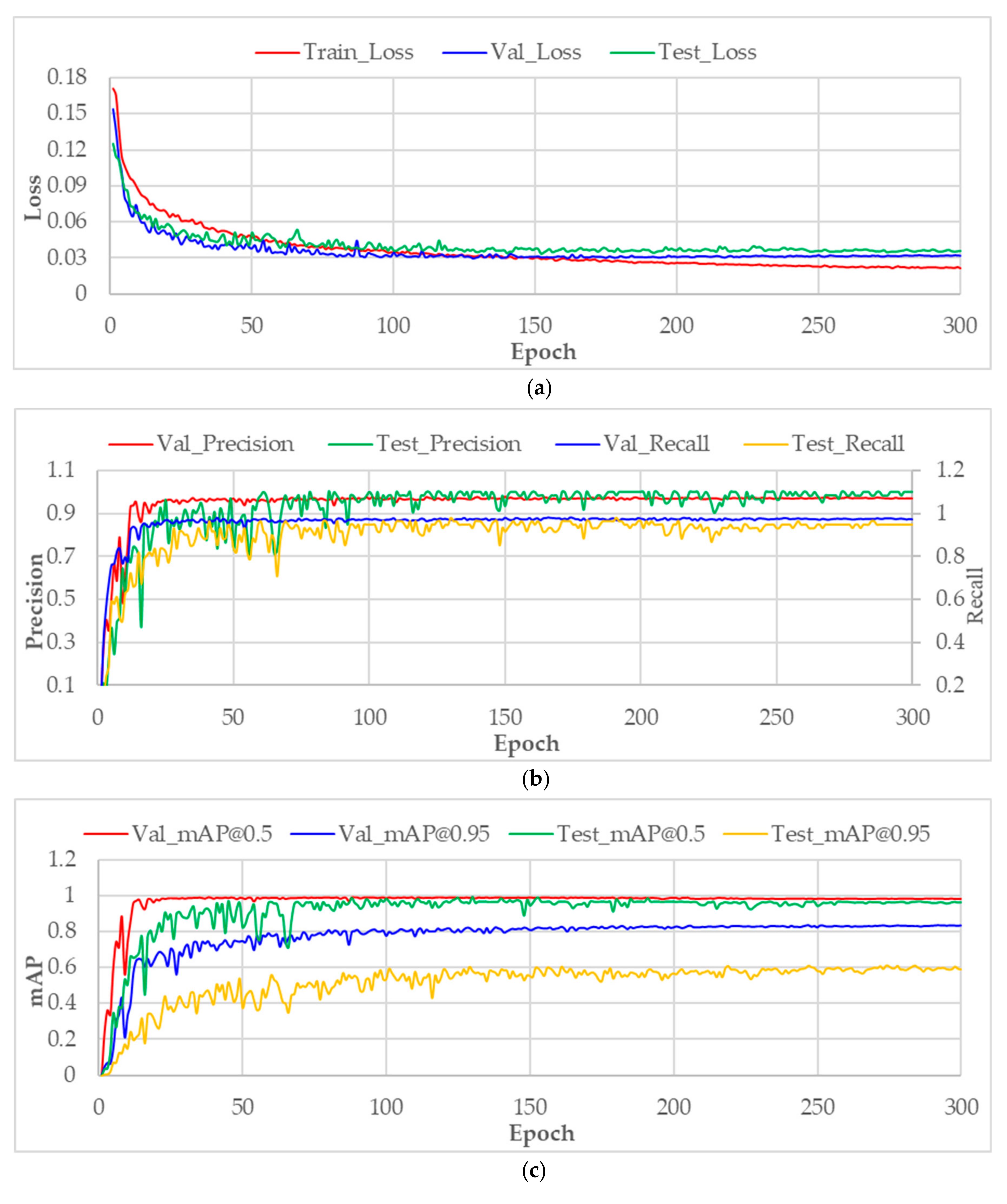
The changes of various indicators during the training process are shown in Figure 20. From about the 100th epoch, the loss values on the validation set and test set tend to stabilize, while the loss value on the training set continues declining slowly, indicating that the fitting of the network to the training set is increasing. At last, the loss has the smallest value on the training set, followed by on the validation, and the largest value on the test set. The precision, recall and mAP of the trained model rise gradually with the increasing training epoch, and also tend to be stable after the 100th epoch. Since the test set is relatively small, the variation curve of these indicators on the test set jitters a little more than on other datasets.
The specific performance statistics of the trained model are shown in Table 2. Although the trained model achieves 100% precision on the test set, the recall is lower than that on the validation set, indicating that the detection model has more missed detections on the test set. There is also a drop of 0.022 in mAP on the test set under the IoU threshold of 0.5 compared to that on the validation set, while under the threshold of 0.95, the mAP on the test set decreases significantly, indicating that there are a considerable number of predicted bounding boxes that have an IoU between 0.5 and 0.95 with the manual annotation; therefore, such a large IoU threshold is not adopted in practical applications. In general, the differences of various indicators between validation set and test set are not significant, which fully demonstrates the effectiveness of the proposed sample synthesis method and the strong generalization ability of the trained model.
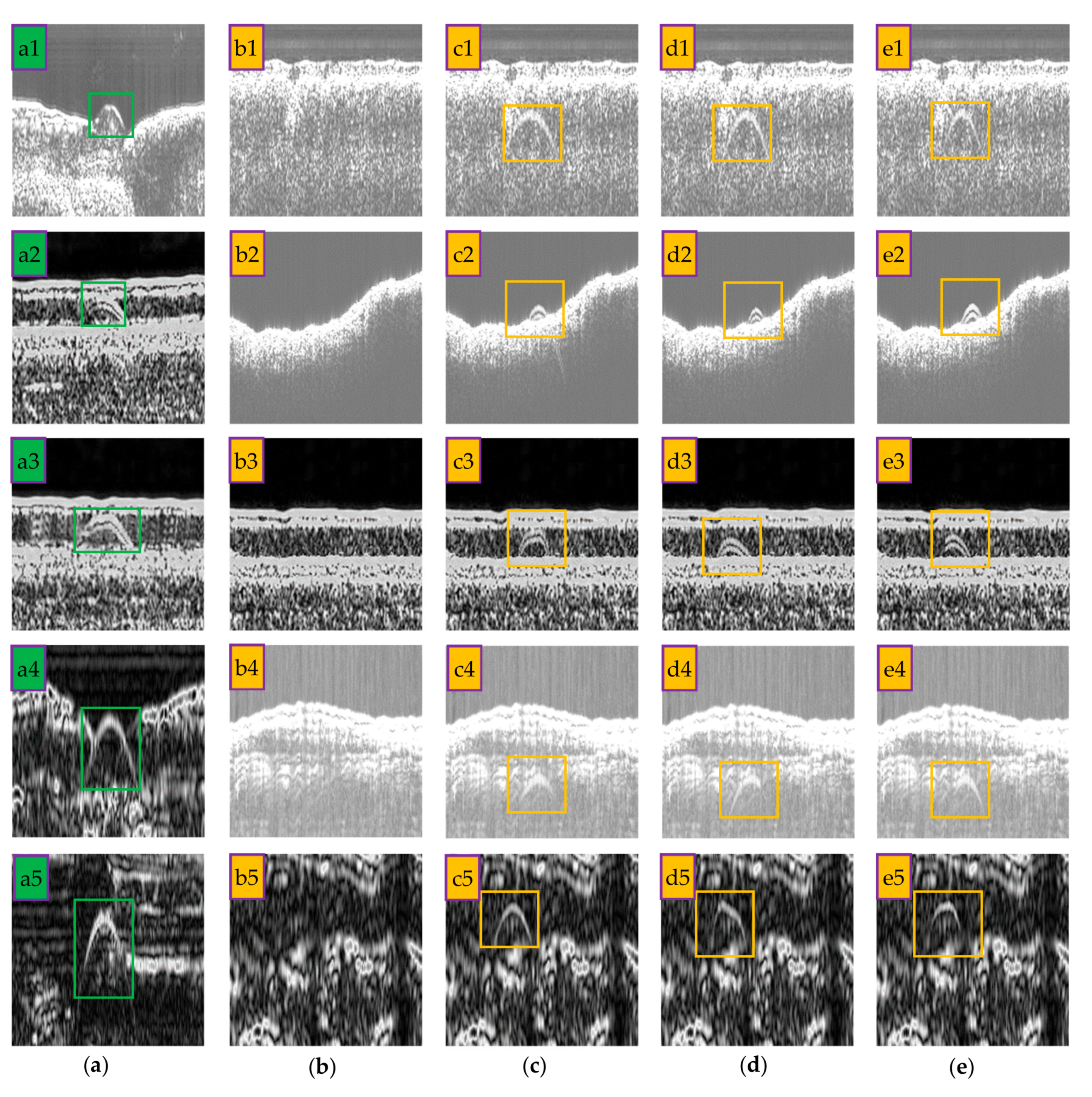
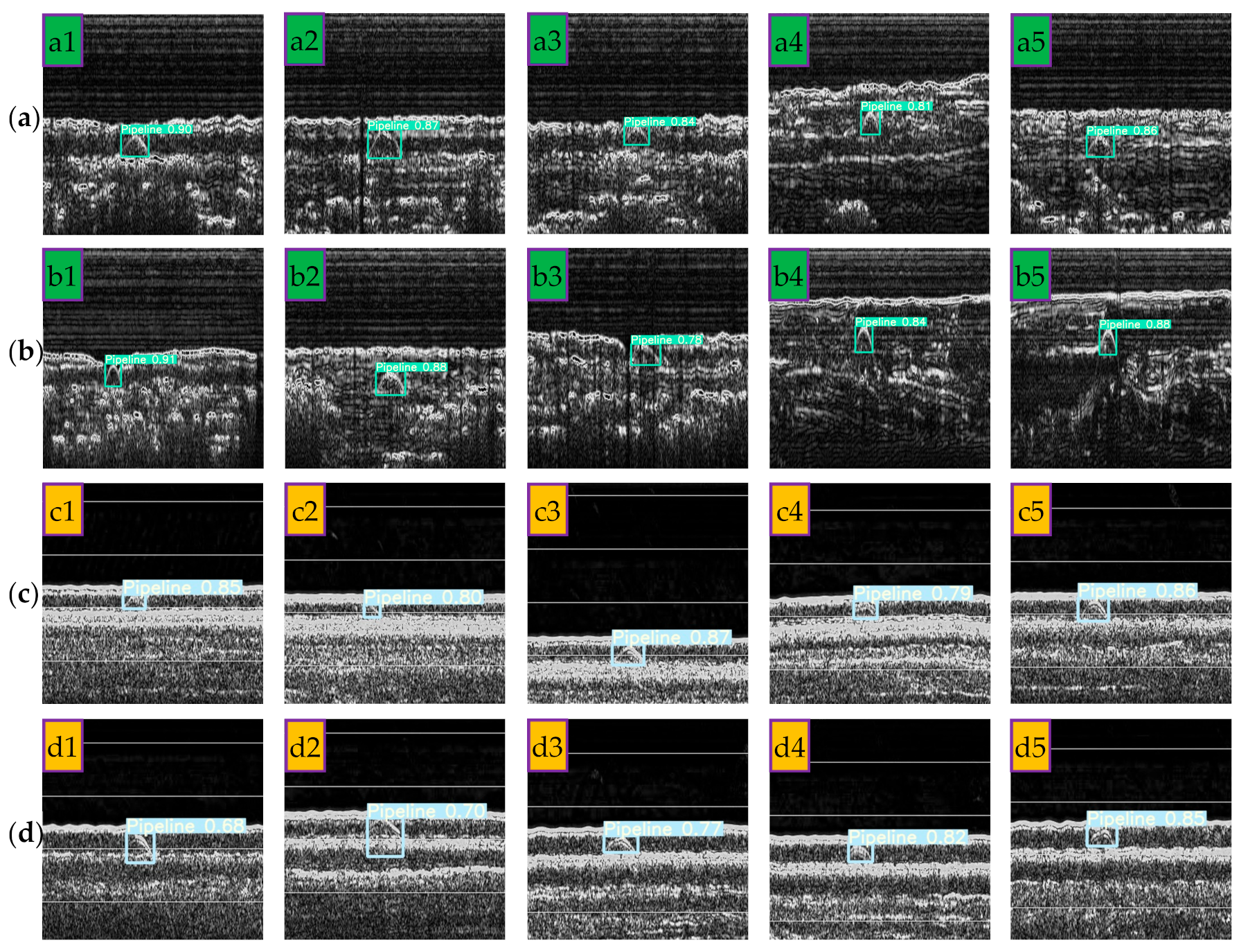
Part of the correct detection results on the test set are shown in Figure 21. Some poorly imaged pipeline targets (a2, a5, b3, c2, c4, d2, etc.) can still be detected, which indicates that the proposed sample synthesis method can well simulate the pipeline imaging results under complex conditions and the trained model has strong pipeline detection capabilities in various SBP images.
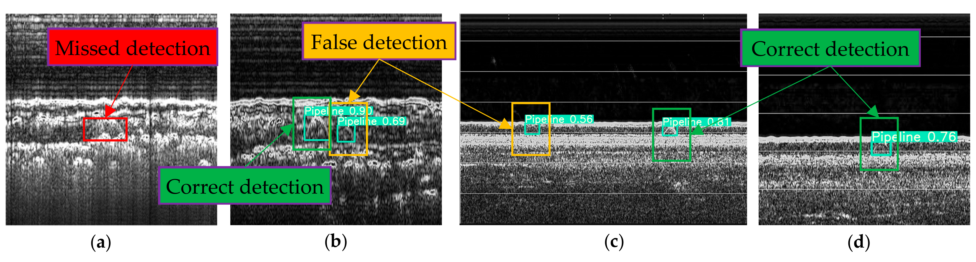
Some of the missed and false detection results are shown in Figure 22. The contrast between the pipeline target in Figure 22a and the background is too low, as a result, the pipeline target in the image is unable to be detected effectively. The false detection targets in Figure 22b,c have high similarity with the real pipeline shapes in appearance, so they are incorrectly recognized as pipelines. For these data, even skilled workers need to make further judgments with the help of historical survey data or magnetic data, and it is understandable that the trained model cannot effectively identify them.
For pipeline investigation, the most important information is the position of the pipeline in the image, which can be obtained from the bounding box predicted by the trained model. In addition, the position prediction deviation (Δx, Δy) can be expressed as:
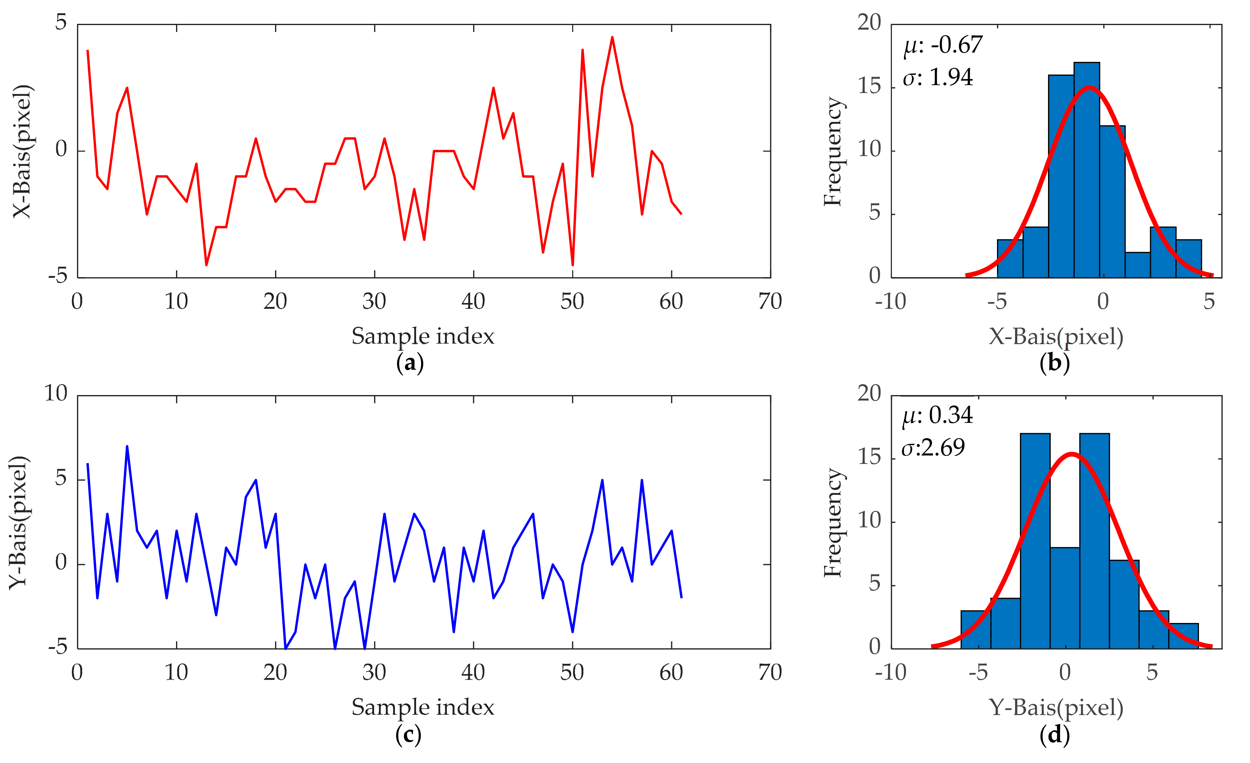
where (xpre, ypre) and hpre is the center coordinate and the height of the predicted bounding box, respectively. (xGT, yGT) and hGT are those of the manual annotation. The pipeline position prediction deviation statistics for each correctly detected sample in the test set are shown in Figure 23. The mean deviation along the x-axis of the image is −0.67 pixels with a standard deviation of 1.94 pixels, corresponding to values of 0.34 and 2.69 along the y-axis. This result shows that the pipeline detection model built in this paper has the potential to completely replace manual measurement.
3.3. Method Comparison
To further validate the generalization capability of the model, a new dataset with 22 samples measured by EdgeTech 3400 in Zhejiang Province of China was used for the experiment. The stratigraphic distribution in the data is significantly different from the data used for sample synthesis, and the state of the pipeline targets is also different from that in the test set. Meanwhile, the latest pipeline detection method proposed in the literature [26] was also implemented as a comparison. The detection results are shown in Table 3.
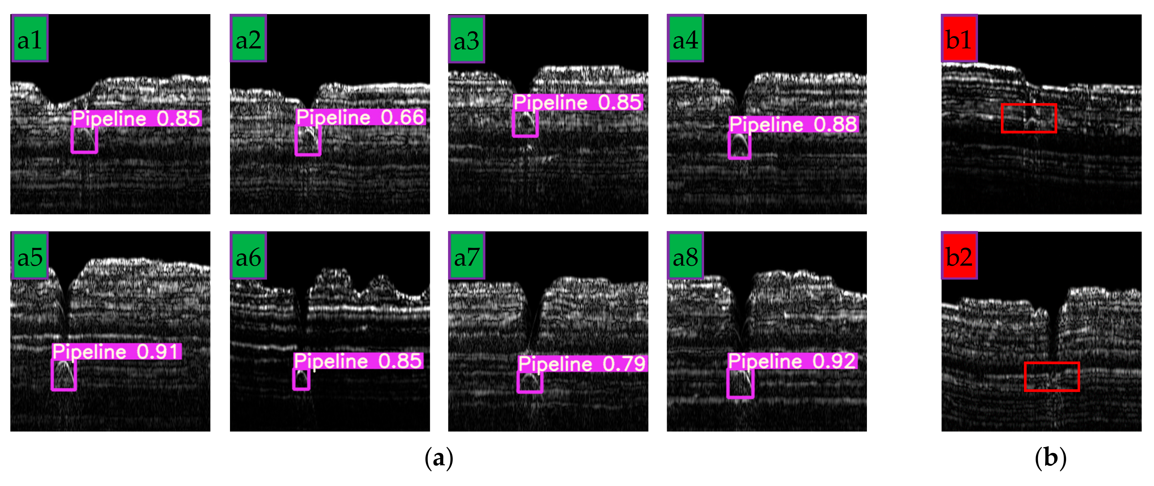
As can be seen from Table 3, even for data measured by different devices in different environments, the trained model still achieves high precision and recall, and outperforms the method proposed in the literature [26]. Some of the correct detection results are shown in Figure 24a. It can be seen that the trained model is able to predict the location of the pipeline with high confidence as well as accuracy, which fully demonstrates the robustness as well as the superiority of the method in this paper. There are two false detection results as shown in Figure 24b. The pipeline in sample b1 is connected to the stratigraphic boundary and has few effective pixels, while the pipeline in b2 is not distinguishable at all. We believe that it is normal for the model to make mistakes in these two cases.
3.4. Real-Time Pipeline Detection
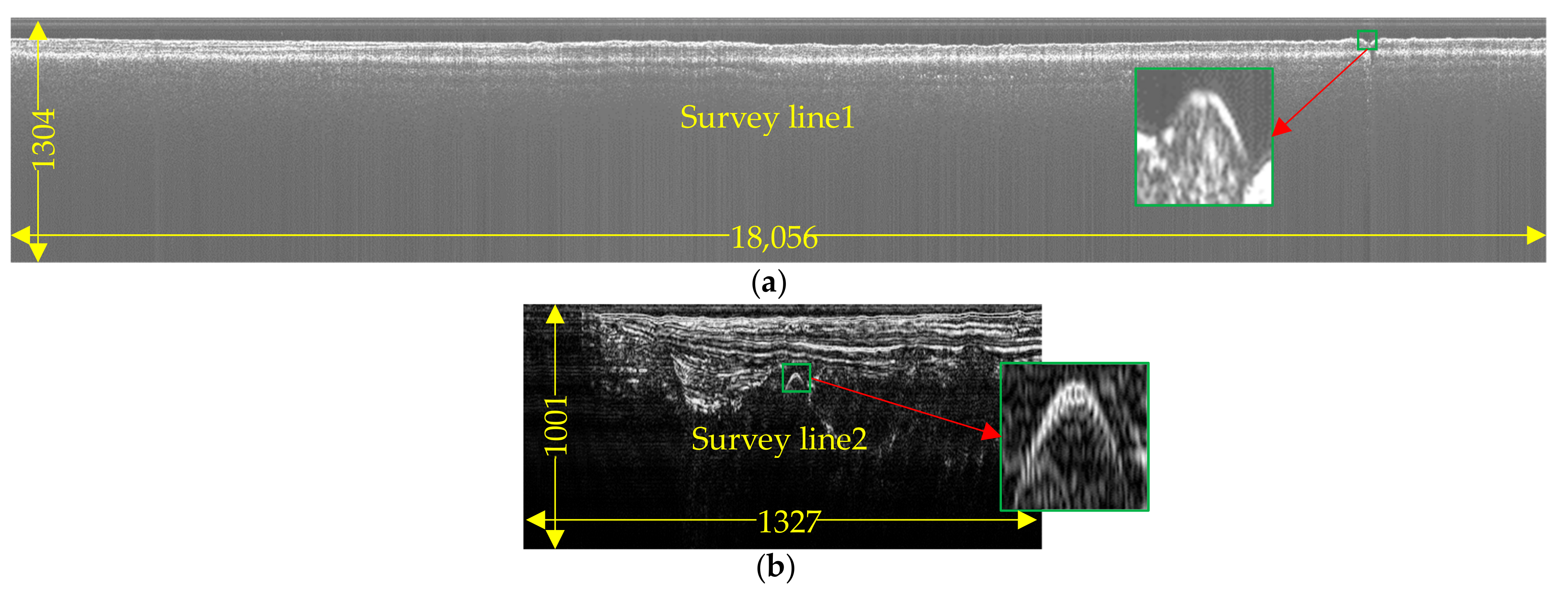
Two complete survey lines of SBP data were used for the real-time pipeline detection experiment, one measured by EdgeTech 3100p in Zhujiang Estuary with 1304 samples per ping for a total of 18,056 pings, and the other measured by Chirp III in Yangtze Estuary, with 1001 samples per ping for a total of 1327 pings, as shown in Figure 25.
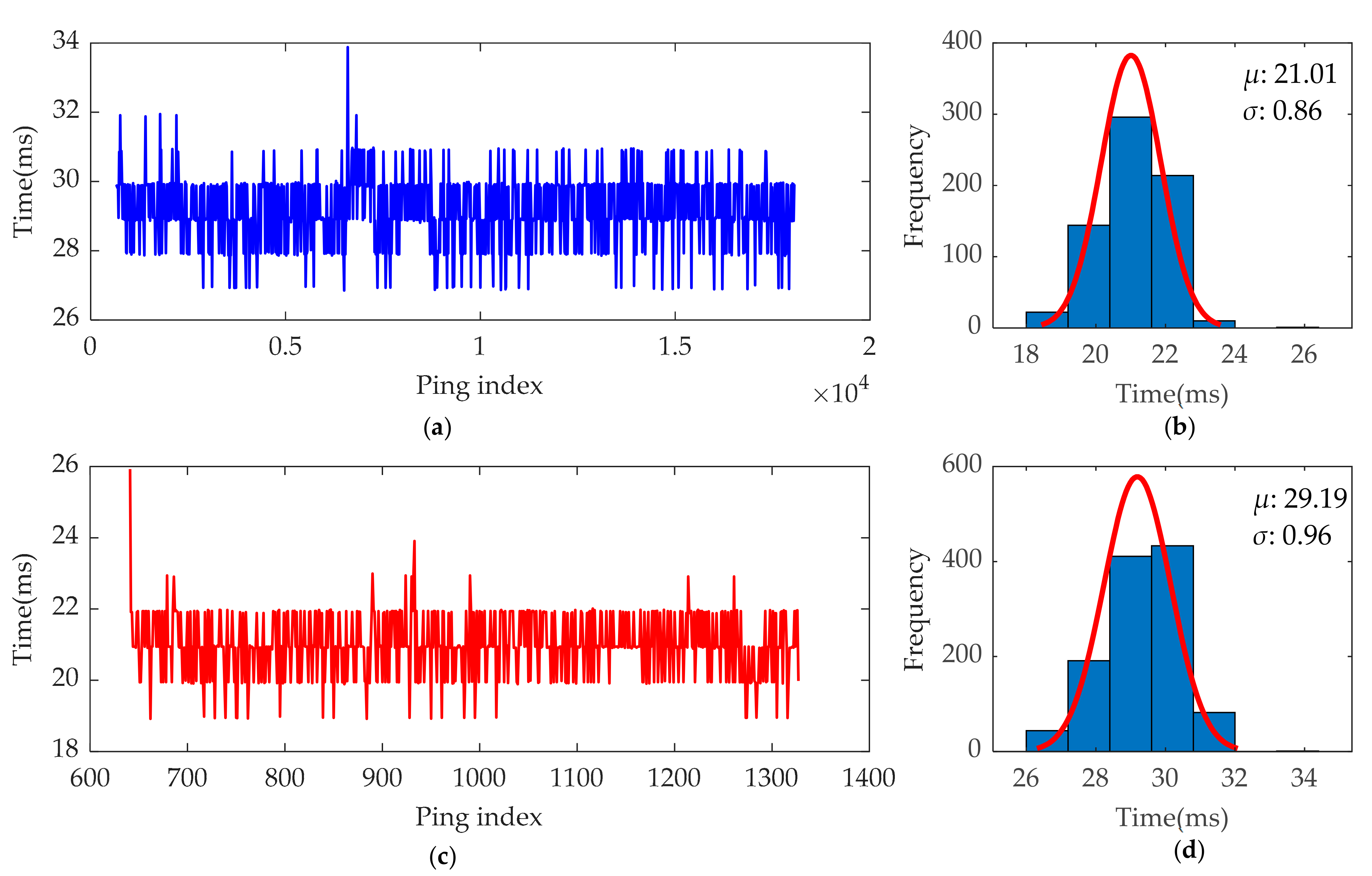
The real-time pipeline detection experiment was carried out on a desktop computer equipped with older hardware (CPU: i7-8700, GPU: GTX1070) according to the method described in Section 2.4.2. In addition, the statistical results of the time spent on each ping are shown in Figure 26.
The object detection time spent on each ping is mainly related to the number of sampling points in the ping. For survey line 1, three sliding windows are detected whenever a new ping arrives, while survey line 2 requires two sliding windows to be detected. Therefore, the time spent per ping in survey line 1 is less than that in survey line 2. The time interval between adjacent pings of SBP data is usually greater than 40 ms, while the average time spent on pipeline detection per ping is 21.01 ms for survey line1 and 29.19 ms for survey line 2, which proves that this method can meet the requirement of real-time detection of pipeline targets.
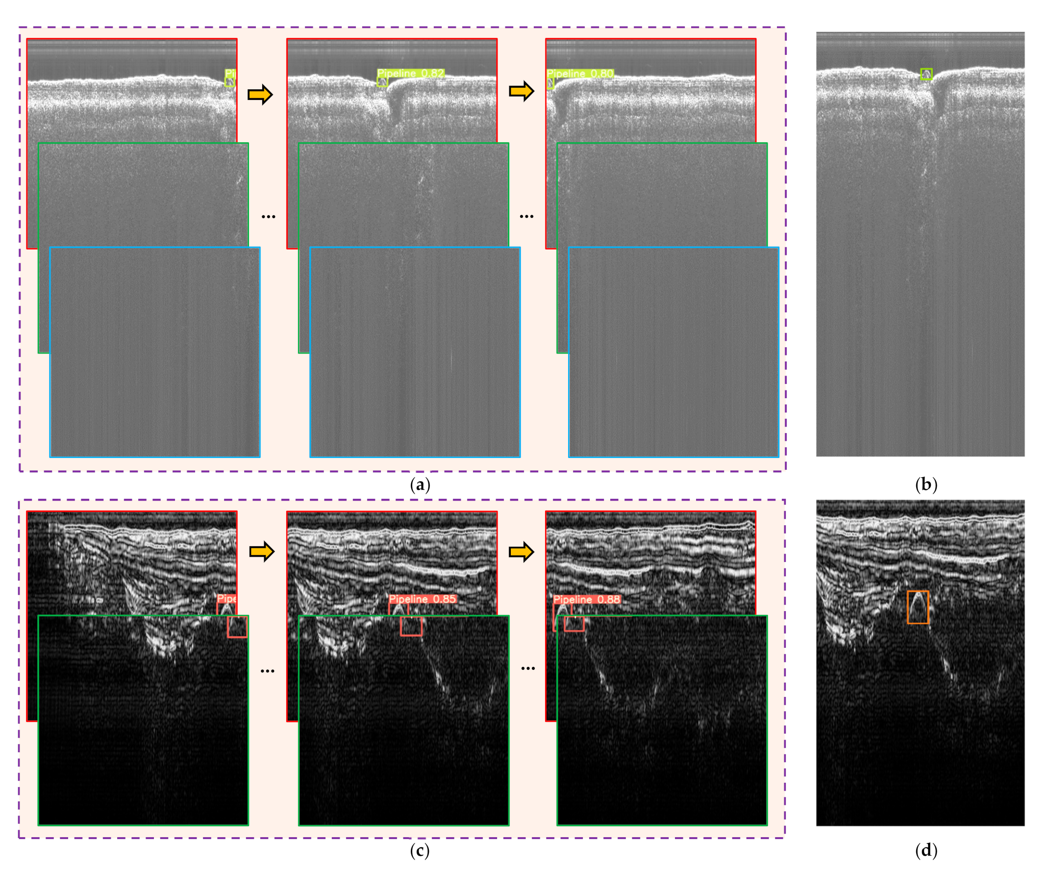
The same target was detected several times during the experiment, and some of the detection results are shown in Figure 27. The detection results were fused according to the method described in Section 2.4.2, and the corresponding results are shown in Figure 27b,d. The pipelines in both survey lines were detected correctly, which proves the effectiveness of the proposed bounding box fusion method.
4. Discussion
4.1. Superiority
Traditional target recognition methods require human extraction of features and selection of classifiers, and the significance of features and the performance of classifiers can directly affect the accuracy of target recognition. The artificial neural network can automatically extract the nonlinear significant features of the target through end-to-end training, and achieve high-precision target recognition with its powerful mapping capability, which is more robust to various complex situations and thus outperforms traditional methods.
However, artificial neural networks require a large number of training samples, and the representativeness of the training samples directly affects the final generalization ability of the trained models. The sample synthesis method proposed in this paper not only considers the SBP imaging principle, but also takes various influencing factors into account. More importantly, it uses the measured data for sample synthesis, so that the synthesized samples retain the real measurement environment and the working characteristics of the measurement instrument. Therefore, the synthesized samples are highly representative of the measured data, which makes it possible to perform object detection based on artificial neural networks in the absence of real samples.
4.2. Efficiency
At present, object detection network can be divided into one-stage (YOLO, SSD, etc.) and two-stage (R-CNN, Faster R-CNN, etc.) networks. Target classification and localization are performed separately in the two-stage networks, while in the one-stage networks, both of the two processes are carried out simultaneously. Therefore, the detection speed of the one-stage network is generally faster. In addition, the real-time detection method designed in this paper is computationally small. While ensuring the integrity of detected targets, there are fewer sliding windows to be detected for each ping, so as to ensure the real-time detection of pipeline.
4.3. Anti-Noise Ability
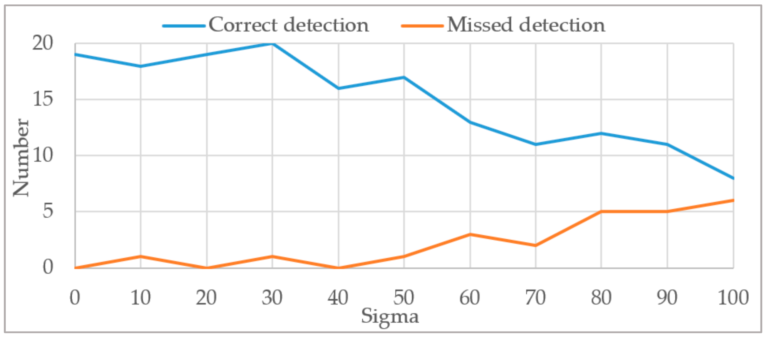
To test the anti-noise ability of the trained model, we apply different levels of Gaussian white noise to the dataset used in Section 3.3 and count the detection results under different noise levels. As shown in Figure 28, when σ ∈ [0, 30], the number of correct and false detections do not change significantly, which indicates that the method in this paper has good resistance to noise. When σ > 30, the number of correct detections gradually decreases and the number of false detections gradually increases.
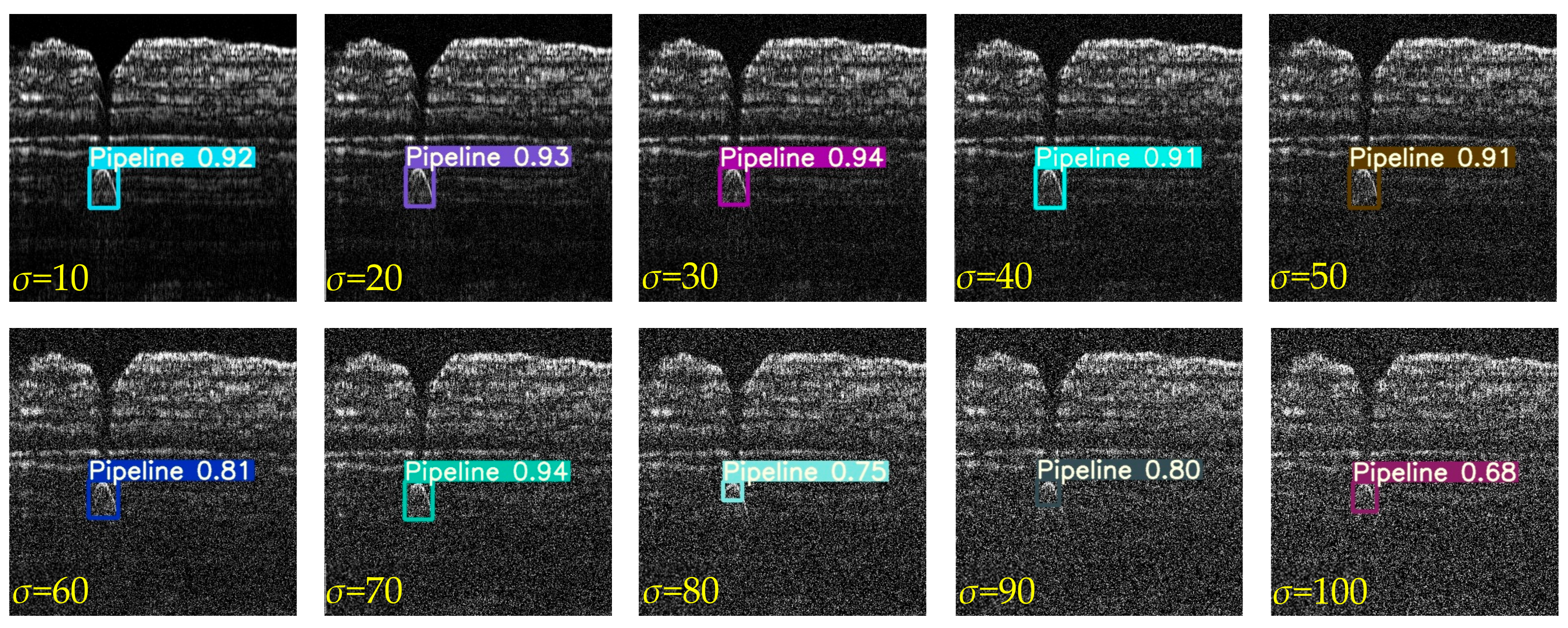
The detection results of a sample under different noise levels with the trained model are shown in Figure 29. With the increase of noise, the confidence of detection results shows a downward trend. Nevertheless, this method can give a robust prediction in a large noise range.
4.4. Exceptional Situations
Although the sample synthesis method proposed in this paper takes into account many influencing factors and the generated samples are highly representative, there are still some cases that can lead to missed and false detections:
- Since the pipeline detection method in this paper is mainly based on the shape characteristics of the pipeline in the SBP image, when the contrast between the pipeline target and the background is so low that it is difficult to distinguish the pipeline visually, the trained model cannot effectively detect the pipeline at this time, and it is necessary to use other survey methods, such as magnetic measurement, to provide more basis for judgment.
- Targets such as independent rocks in stratum and fish in the water will produce similar reflections as the pipeline does, resulting in false detections. At this time, historical survey data or magnetic data are needed to assist decision-making.
4.5. Future Research Directions
From the experiments in this paper, it can be seen that only relying on SBP data for pipeline detection will cause missed and false detections. Future research should combine other measurement data, such as multi-beam bathymetric data and magnetic data to achieve more reliable detection of underwater pipelines.
5. Conclusions
Based on the imaging principles of SBP, a real-time pipeline detection method with zero samples is proposed in this paper. Firstly, an efficient sample synthesis method is proposed to generate highly representative samples. Secondly, the synthesized samples were used for network training. Finally, the trained models were tested on the measured data. The results showed that both the mAP ([email protected]) and the predicted pipeline positions (a mean deviation of −0.67 pixels with a standard deviation of 1.94 pixels along the x-axis, corresponding to values of 0.34 and 2.69 along the y-axis) in the images were comparable to manual interpretation, which fully illustrates the superb representativeness of the synthesized samples and strong generalization ability of the trained model. The experimental results also prove that the proposed method can meet the requirements of real-time pipeline detection of SBP data. The same idea can also be applied to other imaging sonars, such as forward-looking sonar, side-scan sonar, etc., which will greatly promote the development of underwater target detection applications with deep learning methods.
Author Contributions
Conceptualization, G.Z., J.Z. and S.L.; methodology, G.Z.; software, G.Z.; validation, J.Z., S.L. and J.F.; formal analysis, J.Z.; investigation, J.F.; resources, J.Z., S.L. and J.F.; data curation, G.Z.; writing—original draft preparation, G.Z.; writing—review and editing, J.Z.; visualization, G.Z., S.L. and J.F.; supervision, J.Z.; project administration, J.Z.; funding acquisition, J.Z. All authors have read and agreed to the published version of the manuscript.
Funding
This research was funded by National Natural Science Foundation of China under Grant 42176186. This research was also funded by the Key Research & Development Program of New Energy Engineering Limited Company of China Communications Construction Company Third Harbor Engineering Limited Company under Grant 2019-ZJKJ-ZDZX-01-0349 and Class-A project of New Energy Engineering Limited Company of China Communications Construction Company Third Harbor Engineering Limited Company under Grant 2020-04.
Data Availability Statement
Access to the data will be considered upon request by the authors.
Acknowledgments
We would like to thank the editor and anonymous reviewers for their valuable comments and suggestions that greatly improved the quality of this paper. We would also like to thank the open-source project of Ultralytics-YOLOv5.
Conflicts of Interest
The authors declare no conflict of interest.
References
- Kaiser, M.J. A review of deepwater pipeline construction in the U.S. Gulf of Mexico–Contracts, cost, and installation methods. J. Mar. Sci. Appl. 2016, 15, 288–306. [Google Scholar] [CrossRef]
- Hansen, A.S.; Antunes, B.R.; Solano, R.F.; Roberts, G.; Bedrossian, A. Assessment of Lateral Buckles in a HP/HT Pipeline Using Sidescan Sonar Data. In Proceedings of the International Conference on Ocean, Offshore and Arctic Engineering, Rotterdam, The Netherlands, 19–24 June 2011; pp. 897–904. [Google Scholar] [CrossRef]
- Song, S.M.; Li, Y.; Li, Z.G.; Hu, Z.Q.; Li, S.; Cho, G.R.; Li, J.H. Seabed Terrain 3D Reconstruction Using 2D Forward-Looking Sonar: A Sea-Trial Report From The Pipeline Burying Project. Ifac Pap. 2019, 52, 175–180. [Google Scholar] [CrossRef]
- Zhao, X.-F.; Ba, Q.; Li, L.; Gong, P.; Ou, J.-P. A three-index estimator based on active thermometry and a novel monitoring system of scour under submarine pipelines. Sens. Actuators A Phys. 2012, 183, 115–122. [Google Scholar] [CrossRef]
- Tian, W.M. Forensic Investigation of a Breakdown Waste Water Pipeline off Penghu Islands, Taiwan. Aer. Adv. Eng. Res. 2014, 7, 532–535. [Google Scholar]
- Kaiser, M.J. US Gulf of Mexico deepwater pipeline construction—A review of lessons learned. Mar Policy 2017, 86, 214–233. [Google Scholar] [CrossRef]
- Jialei, Z.; Xiang, X. Application of PSO on Electromagnetic Induction-Based Subsea Cable Detection. In Proceedings of the 2019 4th International Conference on Automation, Control and Robotics Engineering, Shenzhen, China, 19–21 July 2019; pp. 1–6. [Google Scholar]
- Lurton, X. An Introduction to Underwater Acoustics: Principles and Applications, 2nd ed.; Springer: New York, NY, USA, 2011; pp. 23–373. [Google Scholar]
- Gauer, R.C.; McFadzean, A.; Reid, C. An automated sidescan sonar pipeline inspection system. Oceans. In Proceedings of the ‘99 Mts/IEEE: Riding the Crest into the 21st Century, Seattle, WA, USA, 13–16 September 1999; Volume 2, pp. 811–816. [Google Scholar]
- Antich, J.; Ortiz, A. Underwater Cable Tracking by Visual Feedback. In Proceedings of the IbPRIA 2003, Puerto de Andratx, Mallorca, Spain, 4–6 June 2003; pp. 53–61. [Google Scholar] [CrossRef]
- Zhang, J.; Xiang, X. Subsea cable tracking by a 5-DOF AUV. In Proceedings of the 2017 36th Chinese Control Conference (CCC), Dalian, China, 26–28 July 2017; pp. 4796–4800. [Google Scholar] [CrossRef]
- Zhang, J.; Zhang, Q.; Xiang, X. Automatic inspection of subsea optical cable by an autonomous underwater vehicle. In Proceedings of the OCEANS 2017, Aberdeen, UK, 19–22 June 2017; pp. 1–6. [Google Scholar] [CrossRef]
- Tian, W.-M. Integrated method for the detection and location of underwater pipelines. Appl. Acoust. 2008, 69, 387–398. [Google Scholar] [CrossRef]
- Xiong, C.B.; Li, Z.; Zhai, G.J.; Lu, H.L. A New Method for Inspecting the Status of Submarine Pipeline Based on a Multi-Beam Bathymetric System. J. Mar. Sci. Tech.-Taiwan 2016, 24, 876–887. [Google Scholar]
- Xiong, C.B.; Li, Z.; Sun, X.; Zhai, J.S.; Niu, Y.B. An Effective Method for Submarine Pipeline Inspection Using Three-Dimensional (3D) Models Constructed from Multisensor Data Fusion. J. Coast. Res. 2018, 34, 1009–1019. [Google Scholar] [CrossRef]
- Guan, M.L.; Cheng, Y.X.; Li, Q.Q.; Wang, C.S.; Fang, X.; Yu, J.W. An Effective Method for Submarine Buried Pipeline Detection via Multi-Sensor Data Fusion. IEEE Access 2019, 7, 125300–125309. [Google Scholar] [CrossRef]
- Liu, Y.; Wang, M.; Cai, Q. The target detection for GPR images based on curve fitting. In Proceedings of the 2010 3rd International Congress on Image and Signal Processing, Yantai, China, 16–18 October 2010; pp. 2876–2879. [Google Scholar]
- Yang, F.; Qiao, X.; Zhang, Y.Y.; Xu, X.L. Prediction Method of Underground Pipeline Based on Hyperbolic Asymptote of OPR Image. In Proceedings of the 2014 15th International Conference on Ground Penetrating Radar (Gpr 2014), Brussels, Belgium, 30 June–4 July 2014; pp. 674–678. [Google Scholar]
- Mertens, L.; Persico, R.; Matera, L.; Lambot, S. Automated Detection of Reflection Hyperbolas in Complex GPR Images With No A Priori Knowledge on the Medium. IEEE Trans. Geosci. Remote Sens. 2015, 54, 580–596. [Google Scholar] [CrossRef]
- Chandra, G.R.; Rajiv, K.; Rao, B.B. A distinctive similarity rendering approach to reconstitute hyperbola apices in GPR images. In Proceedings of the TENCON 2017—2017 IEEE Region 10 Conference, Penang, Malaysia, 5–8 November 2017; pp. 350–353. [Google Scholar] [CrossRef]
- Dou, Q.; Wei, L.; Magee, D.R.; Cohn, A.G. Real-Time Hyperbola Recognition and Fitting in GPR Data. IEEE Trans. Geosci. Remote Sens. 2016, 55, 51–62. [Google Scholar] [CrossRef] [Green Version]
- Zhou, X.; Chen, H.; Li, J. An Automatic GPR B-Scan Image Interpreting Model. IEEE Trans. Geosci. Remote Sens. 2018, 56, 3398–3412. [Google Scholar] [CrossRef]
- Kim, M.; Kim, S.-D.; Hahm, J.; Kim, D.; Choi, S.-H. GPR Image Enhancement Based on Frequency Shifting and Histogram Dissimilarity. IEEE Geosci. Remote Sens. Lett. 2018, 15, 684–688. [Google Scholar] [CrossRef]
- Pasolli, E.; Melgani, F.; Donelli, M. Automatic Analysis of GPR Images: A Pattern-Recognition Approach. IEEE Trans. Geosci. Remote Sens. 2009, 47, 2206–2217. [Google Scholar] [CrossRef]
- Noreen, T.; Khan, U.S. Using Pattern Recognition with HOG to Automatically Detect Reflection Hyperbolas in Ground penetrating Radar Data. In Proceedings of the 2017 International Conference on Electrical and Computing Technologies and Applications (ICECTA), Ras Al Khaimah, United Arab Emirates, 21–23 November 2017; pp. 465–470. [Google Scholar]
- Li, S.; Zhao, J.; Zhang, H.; Zhang, Y. Automatic Detection of Pipelines from Sub-bottom Profiler Sonar Images. IEEE J. Ocean. Eng. 2021, 1–16. [Google Scholar] [CrossRef]
- Wunderlich, J.; Wendt, G.; Müller, S. High-resolution Echo-sounding and Detection of Embedded Archaeological Objects with Nonlinear Sub-bottom Profilers. Mar. Geophys. Res. 2005, 26, 123–133. [Google Scholar] [CrossRef]
- Wang, C.; Jiang, Y.; Wang, K.; Wei, F. A field-programmable gate array system for sonar image recognition based on convolutional neural network. Proc. Inst. Mech. Eng. Part I J. Syst. Control. Eng. 2020, 235, 1808–1818. [Google Scholar] [CrossRef]
- Yu, Y.; Zhao, J.; Gong, Q.; Huang, C.; Zheng, G.; Ma, J. Real-Time Underwater Maritime Object Detection in Side-Scan Sonar Images Based on Transformer-YOLOv5. Remote Sens. 2021, 13, 3555. [Google Scholar] [CrossRef]
- Zheng, G.; Zhang, H.; Li, Y.; Zhao, J. A Universal Automatic Bottom Tracking Method of Side Scan Sonar Data Based on Semantic Segmentation. Remote Sens. 2021, 13, 1945. [Google Scholar] [CrossRef]
- Huo, G.; Wu, Z.; Li, J. Underwater Object Classification in Sidescan Sonar Images Using Deep Transfer Learning and Semisynthetic Training Data. IEEE Access 2020, 8, 47407–47418. [Google Scholar] [CrossRef]
- Bore, N.; Folkesson, J. Modeling and Simulation of Sidescan Using Conditional Generative Adversarial Network. IEEE J. Ocean. Eng. 2020, 46, 195–205. [Google Scholar] [CrossRef]
- Jiang, Y.; Ku, B.; Kim, W.; Ko, H. Side-Scan Sonar Image Synthesis Based on Generative Adversarial Network for Images in Multiple Frequencies. IEEE Geosci. Remote Sens. Lett. 2020, 18, 1505–1509. [Google Scholar] [CrossRef]
- Li, C.; Ye, X.; Cao, D.; Hou, J.; Yang, H. Zero shot objects classification method of side scan sonar image based on synthesis of pseudo samples. Appl. Acoust. 2020, 173, 107691. [Google Scholar] [CrossRef]
- Sub-Bottom Profilers | Geoscience Australia. Available online: https://www.ga.gov.au/scientific-topics/marine/survey-techniques/sonar/shallow-water-sub-bottom-data (accessed on 15 September 2021).
- Sub Bottom Profiler—JW Fishers. Available online: http://jwfishers.com/products/sbp1.html (accessed on 16 September 2021).
- Wang, F.; Ding, J.; Tao, C.; Lin, X. Sound velocity characteristics of unconsolidated sediment based on high-resolution sub-bottom profiles in Jinzhou Bay, Bohai Sea of China. Cont. Shelf Res. 2021, 217, 104367. [Google Scholar] [CrossRef]
- Li, S.; Zhao, J.; Zhang, H.; Bi, Z.; Qu, S. A Non-Local Low-Rank Algorithm for Sub-Bottom Profile Sonar Image Denoising. Remote Sens. 2020, 12, 2336. [Google Scholar] [CrossRef]
- Li, S.; Zhao, J.; Zhang, H.; Qu, S. An Integrated Horizon Picking Method for Obtaining the Main and Detailed Reflectors on Sub-Bottom Profiler Sonar Image. Remote Sens. 2021, 13, 2959. [Google Scholar] [CrossRef]
- Feng, J.; Zhao, J.; Zheng, G.; Li, S. Horizon Picking from SBP Images Using Physicals-Combined Deep Learning. Remote Sens. 2021, 13, 3565. [Google Scholar] [CrossRef]
- Girshick, R.; Donahue, J.; Darrell, T.; Malik, J. Rich feature hierarchies for accurate object detection and semantic segmentation. In Proceedings of the 2014 IEEE Conference on Computer Vision and Pattern Recognition, Columbus, OH, USA, 23–28 June 2014; pp. 580–587. [Google Scholar]
- Liu, W.; Anguelov, D.; Erhan, D.; Szegedy, C.; Reed, S.; Fu, C.Y.; Berg, A.C. SSD: Single Shot MultiBox Detector. In Proceedings of the Computer Vision—ECCV 2016, Amsterdam, The Netherlands, 11–14 October 2016; Volume 9905, pp. 21–37. [Google Scholar]
- Ren, S.Q.; He, K.M.; Girshick, R.; Sun, J. Faster R-CNN: Towards Real-Time Object Detection with Region Proposal Networks. IEEE Trans. Pattern Anal. 2017, 39, 1137–1149. [Google Scholar] [CrossRef] [Green Version]
- Redmon, J.; Farhadi, A. YOLOv3: An Incremental Improvement. arXiv 2018, arXiv:1804.02767. [Google Scholar]
- Wang, C.-Y.; Liao, H.-y.; Wu, Y.-H.; Chen, P.-Y.; Hsieh, J.-W.; Yeh, I.H. CSPNet: A New Backbone that can Enhance Learning Capability of CNN. In Proceedings of the 2020 IEEE/CVF Conference on Computer Vision and Pattern Recognition, Seattle, WA, USA, 14–19 June 2020; pp. 1571–1580. [Google Scholar]
- Rezatofighi, H.; Tsoi, N.; Gwak, J.; Sadeghian, A.; Reid, I.; Savarese, S. Generalized Intersection over Union: A Metric and A Loss for Bounding Box Regression. In Proceedings of the 2019 IEEE/Cvf Conference on Computer Vision and Pattern Recognition (Cvpr 2019), Long Beach, CA, USA, 15–20 June 2019; pp. 658–666. [Google Scholar]
- GitHub—ultralytics/yolov5: YOLOv5 in PyTorch > ONNX > CoreML > TFLite. Available online: https://github.com/ultralytics/yolov5 (accessed on 15 September 2021).
Figure 1.
SBP working principle. (a) Echo signal generation process; (b) measured SBP waterfall image with a pipeline target.
Figure 1.
SBP working principle. (a) Echo signal generation process; (b) measured SBP waterfall image with a pipeline target.

Figure 2.
Pipeline imaging mechanism. (a) Pipeline shape formation process; (b) geometric relationship between the pipeline and the transducer when the transmitted acoustic signal reaches the pipeline.
Figure 2.
Pipeline imaging mechanism. (a) Pipeline shape formation process; (b) geometric relationship between the pipeline and the transducer when the transmitted acoustic signal reaches the pipeline.

Figure 3.
Influence of various factors on pipeline images. (a–f) are measured pipeline images disturbed by some common influencing factors.
Figure 3.
Influence of various factors on pipeline images. (a–f) are measured pipeline images disturbed by some common influencing factors.

Figure 4.
A ping of raw echo data recorded by SBP and the analytic signal envelope.

Figure 5.
Interpolation process of the raw SBP waterfall image. (a) Select two adjacent pings in order; (b) calculate the actual distance of each ping relative to the first ping along the track; (c) calculate the corresponding image range between the two pings and perform interpolation calculation for each pixel in the range based on the average vertical resolution rv.

Figure 6.
Raw SBP waterfall image interpolation. (a) Raw waterfall image collected by C-boom; (b) interpolated image.
Figure 6.
Raw SBP waterfall image interpolation. (a) Raw waterfall image collected by C-boom; (b) interpolated image.

Figure 7.
Pipeline sample synthesis flow chart.

Figure 8.
Noise separation of SBP image with the non-local low-rank algorithm. (a) Waterfall image disturbed by noise; (b) de-noised image; (c) noise image.
Figure 8.
Noise separation of SBP image with the non-local low-rank algorithm. (a) Waterfall image disturbed by noise; (b) de-noised image; (c) noise image.

Figure 9.
Influence of directivity pattern on pipeline imaging. (a) Examples of transducer directivity pattern; (b) energy variation of the sound pulse hitting the pipeline during the movement of the transducer.
Figure 9.
Influence of directivity pattern on pipeline imaging. (a) Examples of transducer directivity pattern; (b) energy variation of the sound pulse hitting the pipeline during the movement of the transducer.

Figure 10.
Examples of pipeline shape in the pre-processed SBP image. (a) Pipeline diameter is less than SBP resolution; (b) pipeline diameter is larger than the SBP resolution. k is the pixel index relative to the first pipeline echo in each column of the image. The empty spaces in the pipeline image are the gaps between echoes from the upper and lower surfaces of the pipeline. ns is the number of the pixels produced by the echo signal from the pipeline.

Figure 11.
Influence of pulse duration on pipeline echo signal. (a) Reflection of acoustic pulses by pipelines; (b) variation of echo signal with time at different pulse lengths.
Figure 11.
Influence of pulse duration on pipeline echo signal. (a) Reflection of acoustic pulses by pipelines; (b) variation of echo signal with time at different pulse lengths.

Figure 12.
Simulation of the pipeline echo variation in a certain column of the image. (a) There is signal aliasing; (b) the pipeline diameter is greater than the propagation distance of sound waves within the effective pulse duration.
Figure 12.
Simulation of the pipeline echo variation in a certain column of the image. (a) There is signal aliasing; (b) the pipeline diameter is greater than the propagation distance of sound waves within the effective pulse duration.

Figure 13.
Pipeline echo intensity determination with the measured SBP data. (a) Waterfall image generated from measured SBP Data; (b) echoes from the interfaces between layers (the white part of the image).
Figure 13.
Pipeline echo intensity determination with the measured SBP data. (a) Waterfall image generated from measured SBP Data; (b) echoes from the interfaces between layers (the white part of the image).

Figure 14.
Pipeline image generated according to the theoretical formula. (a) Pipeline image with signal aliasing; (b) pipeline image without signal aliasing.
Figure 14.
Pipeline image generated according to the theoretical formula. (a) Pipeline image with signal aliasing; (b) pipeline image without signal aliasing.

Figure 15.
Pipeline images after applying various factors. (a,b) are only influenced by the heave of the carrier platform; (c,d) suffer both the heave of the carrier platform and missing effective pipeline echoes.
Figure 15.
Pipeline images after applying various factors. (a,b) are only influenced by the heave of the carrier platform; (c,d) suffer both the heave of the carrier platform and missing effective pipeline echoes.

Figure 16.
A generated pipeline sample. (a) Bounding box obtained during the sample synthesis process; (b) bounding box with manual optimization.
Figure 16.
A generated pipeline sample. (a) Bounding box obtained during the sample synthesis process; (b) bounding box with manual optimization.

Figure 17.
YOLO5s structure. (a) The backbone; (a) the neck; (c) the output.

Figure 18.
Schematic diagram of real-time pipeline inspection process.

Figure 19.
Sample synthesis results with the proposed method. (a) Measured pipeline images; (b) measured SBP images without pipeline targets; (c–e) synthesized samples with different parameter settings.
Figure 19.
Sample synthesis results with the proposed method. (a) Measured pipeline images; (b) measured SBP images without pipeline targets; (c–e) synthesized samples with different parameter settings.

Figure 20.
Variation in various indicators during the training. (a) Loss curves on training set, validation set and test set; (b) variation in precision and recall on validation set and test set; (c) variation of mAP on validation set and test set under the IoU thresholds of 0.5 and 0.95.
Figure 20.
Variation in various indicators during the training. (a) Loss curves on training set, validation set and test set; (b) variation in precision and recall on validation set and test set; (c) variation of mAP on validation set and test set under the IoU thresholds of 0.5 and 0.95.

Figure 21.
Part of the correct detection results on the test set. (a,b) Pipeline images collected by Chirp III; (c,d) pipeline images collected by EdgeTech 3200XS.
Figure 21.
Part of the correct detection results on the test set. (a,b) Pipeline images collected by Chirp III; (c,d) pipeline images collected by EdgeTech 3200XS.

Figure 22.
False detection and missed detection results. (a) Missed detection; (b) false detection; (c) false detection; (d) correct detection.
Figure 22.
False detection and missed detection results. (a) Missed detection; (b) false detection; (c) false detection; (d) correct detection.

Figure 23.
Statistical results of pipeline position deviations. (a) Deviation along the x-axis of the image; (b) deviation distribution along the x-axis; (c) deviation along the y-axis of the image; (d) deviation distribution along the y-axis.
Figure 23.
Statistical results of pipeline position deviations. (a) Deviation along the x-axis of the image; (b) deviation distribution along the x-axis; (c) deviation along the y-axis of the image; (d) deviation distribution along the y-axis.

Figure 24.
Part of the correct detection results of the proposed method. (a) Part of the correct detection results; (b) missed detection results.
Figure 24.
Part of the correct detection results of the proposed method. (a) Part of the correct detection results; (b) missed detection results.

Figure 25.
Complete survey lines for real-time pipeline detection experiment. (a) SBP data collected by EdgeTech 3100P in Zhujiang Estuary; (b) SBP data collected by Chirp III in Yangtze Estuary.
Figure 25.
Complete survey lines for real-time pipeline detection experiment. (a) SBP data collected by EdgeTech 3100P in Zhujiang Estuary; (b) SBP data collected by Chirp III in Yangtze Estuary.

Figure 26.
Statistical results of the time spent on pipeline detection for each ping. (a) Pipeline detection time spent on each ping of survey line 1; (b) pipeline detection time distribution for each ping of survey line 2; (c) pipeline detection time spent on each ping of survey line 2; (d) distribution of the time spent on each ping of survey line 2.

Figure 27.
Part of the real-time detection results of the two survey lines. (a) Part of the detection results of the same pipeline in survey line 1; (b) bounding box fusion result of the pipeline in survey line 1; (c) part of the detection results of the same pipeline in survey line 2; (d) bounding box fusion result of the pipeline in survey line 2.

Figure 28.
Variation of detection results with increasing noise.

Figure 29.
Detection results of the same sample at different noise levels.


Table 1.
Variable values used in sample synthesis.
| Variable Name | Value | Unit |
|---|---|---|
| θbw | [5, 15] | 1 |
| Dmin | [5, 25] | m |
| R | [0.2, 0.8] | m |
| γ | [0.001, 0.1] | Neper/km |
| Ts | [20, 120] | μs |
| Te | [40, 240] | μs |
| c | 1600 | m/s |
| β | [0.3, 1.2] | - 1 |
| Ai | [0, 10] | pixel |
| ωi | [0.01, 0.1] | rad/pixel |
| φi | [0, 2π] | rad |
| M | [0, 40] | % |
1 Dimensionless.
Table 2.
Performance statistics of the trained model on validation set and test set.
| Dataset | Precision | Recall | [email protected] 1 | [email protected] 2 |
|---|---|---|---|---|
| Validation set | 97.4% | 97.3% | 0.984 | 0.836 |
| Test set | 100% | 95.2% | 0.962 | 0.589 |
1 mAP under the IoU threshold of 0.5. 2 mAP under the IoU threshold of 0.95.
Table 3.
Performance statistics of different methods.
| Method | Correct Detection | False Detection | Precision | Recall |
|---|---|---|---|---|
| Li et al. | 19 | 2 | 90.5% | 86.4% |
| Ours | 20 | 0 | 100% | 90.0% |
Publisher’s Note: MDPI stays neutral with regard to jurisdictional claims in published maps and institutional affiliations. |
© 2021 by the authors. Licensee MDPI, Basel, Switzerland. This article is an open access article distributed under the terms and conditions of the Creative Commons Attribution (CC BY) license (https://creativecommons.org/licenses/by/4.0/).
Share and Cite
MDPI and ACS Style
Zheng, G.; Zhao, J.; Li, S.; Feng, J. Zero-Shot Pipeline Detection for Sub-Bottom Profiler Data Based on Imaging Principles. Remote Sens. 2021, 13, 4401. https://0-doi-org.brum.beds.ac.uk/10.3390/rs13214401
AMA Style
Zheng G, Zhao J, Li S, Feng J. Zero-Shot Pipeline Detection for Sub-Bottom Profiler Data Based on Imaging Principles. Remote Sensing. 2021; 13(21):4401. https://0-doi-org.brum.beds.ac.uk/10.3390/rs13214401
Chicago/Turabian StyleZheng, Gen, Jianhu Zhao, Shaobo Li, and Jie Feng. 2021. "Zero-Shot Pipeline Detection for Sub-Bottom Profiler Data Based on Imaging Principles" Remote Sensing 13, no. 21: 4401. https://0-doi-org.brum.beds.ac.uk/10.3390/rs13214401
Note that from the first issue of 2016, this journal uses article numbers instead of page numbers. See further details here.