Bagging and Boosting Ensemble Classifiers for Classification of Multispectral, Hyperspectral and PolSAR Data: A Comparative Evaluation

Abstract

In recent years, several powerful machine learning (ML) algorithms have been developed for image classification, especially those based on ensemble learning (EL). In particular, Extreme Gradient Boosting (XGBoost) and Light Gradient Boosting Machine (LightGBM) methods have attracted researchers’ attention in data science due to their superior results compared to other commonly used ML algorithms. Despite their popularity within the computer science community, they have not yet been well examined in detail in the field of Earth Observation (EO) for satellite image classification. As such, this study investigates the capability of different EL algorithms, generally known as bagging and boosting algorithms, including Adaptive Boosting (AdaBoost), Gradient Boosting Machine (GBM), XGBoost, LightGBM, and Random Forest (RF), for the classification of Remote Sensing (RS) data. In particular, different classification scenarios were designed to compare the performance of these algorithms on three different types of RS data, namely high-resolution multispectral, hyperspectral, and Polarimetric Synthetic Aperture Radar (PolSAR) data. Moreover, the Decision Tree (DT) single classifier, as a base classifier, is considered to evaluate the classification’s accuracy. The experimental results demonstrated that the RF and XGBoost methods for the multispectral image, the LightGBM and XGBoost methods for hyperspectral data, and the XGBoost and RF algorithms for PolSAR data produced higher classification accuracies compared to other ML techniques. This demonstrates the great capability of the XGBoost method for the classification of different types of RS data.

1. Introduction

Earth observations (EO) image classification is one of the most widely used analysis techniques in the remote sensing (RS) community. Image classification techniques are used to automatically and analytically interpret a significant amount of data from various EO sensors for diverse applications, such as change detection, crop mapping, forest monitoring, and wetland classification [1,2]. Thanks to the unique characteristics of EOs, which provide spatial, spectral, temporal, and polarimetric information, they have been frequently used in classification tasks for mapping various land use/land covers (LULC). To improve the classification accuracy of remotely sensed imagery, the application of multi-source EO data collected using different portions of the electromagnetic spectrum has been extensively increased in the past decade [3].

In general, satellite image classification methods in the RS community can be categorized as two major types: unsupervised algorithms and supervised algorithms [4,5]. The former group is associated with the methods in which there is no need to have prior knowledge and labeled patterns of the study area. The latter group includes methods that use prior knowledge and manually designed features of the study area [5]. Ensemble learning (EL) methods or multiple classifier systems are among supervised classification approaches that combine multiple learners, which improve predictive performance compared to utilizing a single classifier (see Figure 1).

The core idea behind EL methods is to assemble “weak learners” to create a “robust learner” in order to achieve a better classification result [6,7]. In other words, since the EL methods are based on one classification algorithm as the base classifier, to improve the classification result, several diverse algorithms are combined. Note that in this case, the difference between various classifiers is not considered, and this is a key disadvantage of such techniques [8,9]. EL approaches have been recently used in RS applications for improving the LULC classification results [10] and for overcoming the instability of some ML classifiers [11].

Bagging (acronym for Bootstrap AGGregatING) and boosting are two families of the most commonly used integrated or so-called ensemble decision tree classifiers [12,13], which are based on manipulating training samples [14]. Bagging is a kind of regular ensemble classifier technique in which several predictors are made independently and combined using some model averaging methods such as weighted average or majority vote [15]. In contrast, Boosting is an EL technique in which the models are not built independently but sequentially, and successive predictors are used in an attempt to correct the errors generated by previous predictors [16,17]. There are some essential differences between Bagging and Boosting techniques that are listed in

Table 1. Main differences between Bagging and Boosting.

Bagging	Boosting
Predictors/models are independent of each other.	Predictors/models are not independent of each other.
There is no concept of learning from each other.	Each of the individual predictors in the chain learns to fix or minimize the prediction error of the previous one while moving sequentially forward.
Aims to decrease variance.	Seeks to lower the bias.

.

Random Forest (RF) is one of the most well-known, commonly used Bagging techniques for RS image classification in a variety of applications [18]. Additionally, over the last two decades, several decision-tree-based boosting algorithms have been introduced, which paved the way for data analysis. Adaptive boosting (AdaBoost), Gradient boosting machine (GBM), Extreme gradient boosting (XGBoost), and Light gradient boosting machine (LightGBM) are among the methods that fall under the category of Boosting techniques in EL. XGBoost and LightGBM methods are examples of the new generation EL algorithms and have been used in RS in the recent years [19,20,21]. For instance, Georganos et al., (2018) compared XGBoost with other classifiers, such as support vector machine (SVM), RF, k-nearest neighborhood, and recursive partitioning methods for land cover classification using high-resolution satellite imagery [19]. They applied several feature selection algorithms to evaluate the performance of ML classifiers in terms of accuracy. Their study concluded that the XGBoost method achieves high accuracy with fewer features. Shi et al., (2019) evaluated the performance of the LightGBM method in the classification of airborne LiDAR point cloud data in urban areas [22] and showed the effectiveness of EL approaches.

A comparison of XGBoost and RF algorithms’ performance in the process of early-season mapping of sugarcane was conducted in [23] using sentinel-1 imagery time series. Their results indicated that the XGBoost accuracy in detecting target areas was slightly lower than the RF accuracy, but its computation speed is several times faster. Moorthy et al., (2020) assessed the performances of three different supervised models, namely RF, XGBoost, and LightGBM methods for classifying leaf and wooded areas using LiDAR point cloud data of forests [24].

Zhong et al., (2019) made use of deep learning, XGBoost, SVM, and RF methods for the classification of agricultural products [25]. Among non-deep-learning classifiers that they used, XGBoost produced the best outcomes and its accuracy was slightly lower than the proposed deep learning model. Saini and Ghosh (2019) used Sentinel-2 images in their study and compared the efficiency of XGBoost, RF, and SVM algorithms in crop classification of agricultural environment [26]. They verified the outperformance of XGBoost method over the rest of the classifiers. In a study conducted by Dey et al., (2020), they used RF and XGBoost classifiers for crop-type mapping using full polarimetric Radarsat-2 PolSAR satellite images [27]. Based on their assessment in two different case studies, the accuracy of XGBoost is strongly higher than RF. In [28], Gašparovic and Dobrinic analyzed various ML methods, including RF, SVM, XGBoost, and AdaBoost for urban vegetation mapping using multitemporal Sentinel-1 imagery and concluded that SVM and AdaBoost achieved higher accuracy than the other models.

Overall, and according to the reported literature, the ensemble classifiers have the possibility to be utilized in a wide range of RS applications and LULC mapping. It is concluded that the bagging and boosting methods such as RF, XGBoost and LightGBM have remarkable performance relative to other ML approaches. The objective of this study is to evaluate six different ML methods for classifying RS data. Some of the newly proposed EL methods (e.g., XGBoost and LightGBM) are limited in applications to date. Therefore, a comparative evaluation of the prediction power of these techniques is necessary to guide application-oriented research. To the best of our knowledge, a comparative evaluation of the possibility of utilizing these two EL categories (i.e., bagging and boosting methods) in the classification of various RS data does not yet appear in the literature. Therefore, in this paper, we aim at analyzing and comparing some of the well-known approaches to deal with the classification of the three most popular and widely used benchmark RS datasets.

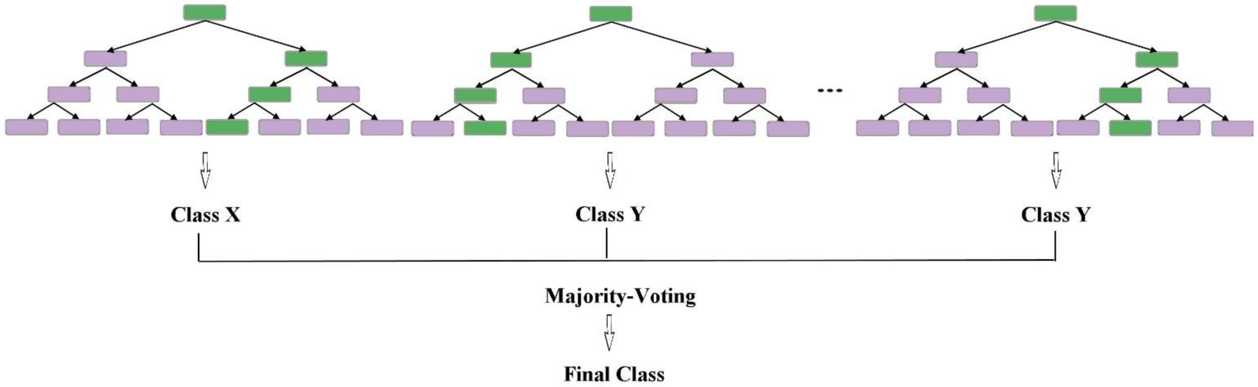
2. Ensemble Learning Classifiers

In the bagging algorithms, the model is built on bootstrap replicates of the original training dataset with replacement. Each training data replica is then used in a classification iteration using a ML algorithm (e.g., DT). To assign classes’ labels, the outputs from all iterations are combined, by taking the average or voting principle [13]. The bagging approach does not weight the samples. Rather, all classifiers in the bagging algorithm are given equal weights during the voting [14].

As intimated in the introduction, the Boosting algorithm is a general supervised technique that utilizes an iterative re-training procedure in which the weights of the incorrectly classified observations are reduced, and the correct predictions receive more weight during a successive iteration. Unlike bagging, the classifiers’ votes in boosting are entirely dependent on their relative accuracy performance [14,29], and this decreases the variance and bias in the classification task [11]. This could lead to more accuracy in results compared to other EL techniques. Despite these benefits and their accurate results, some of the Boosting methods like GBM are generally noise sensitivity and demand high computational cost [14].

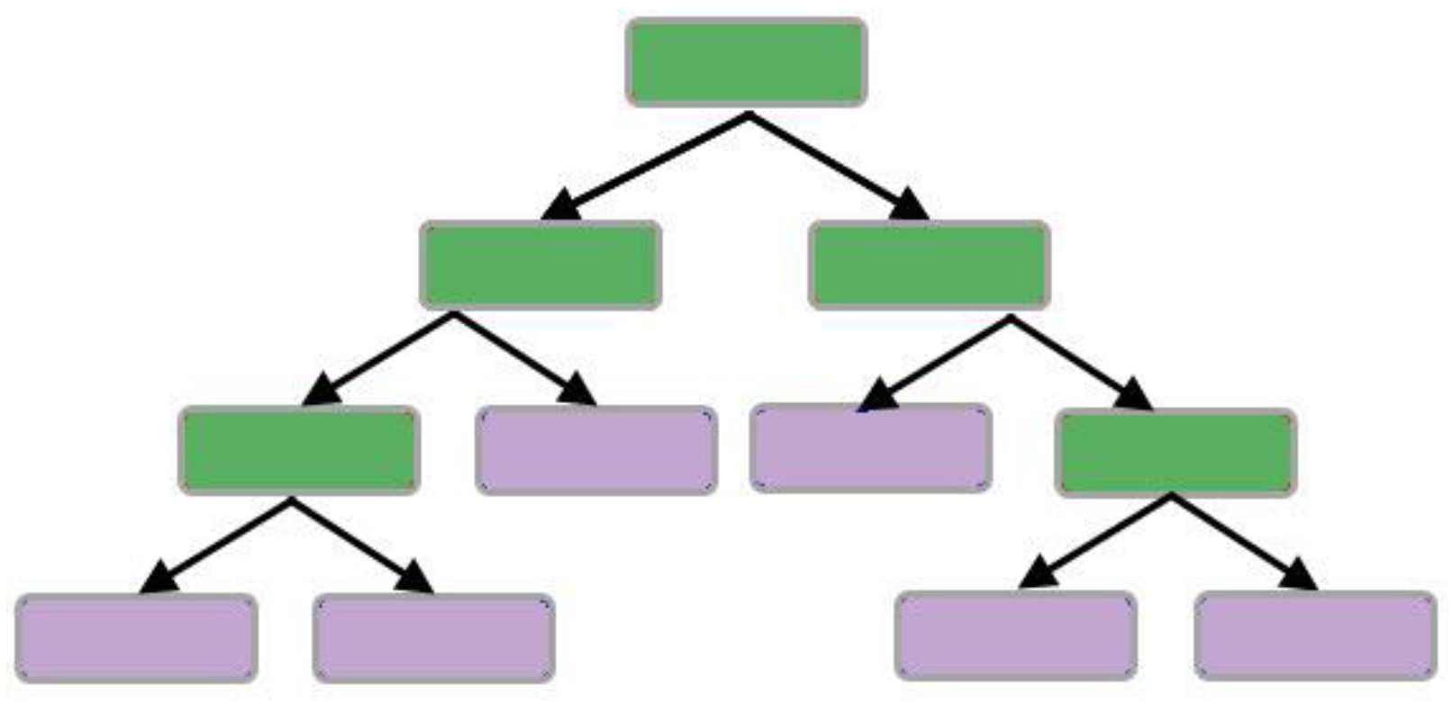
2.1. Decision Tree (DT)

DT is a non-parametric, simple structure classification algorithm with an ability to control nonlinear relations between features and classes [30]. In particular, DT is a tree-based hierarchy of rules and can be defined as a procedure that partitions/splits the input data into smaller and smaller subsets recursively [30,31]. The splitting process is based on a set of thresholds delineated in each of the internal nodes in the tree (see Figure 2). Internal nodes split input data from the root node—the first node in the DT- into sub-nodes, and split sub-nodes into further sub-nodes [30,32]. Through this sequentially binary subdivision, the input data are classified in which the end of nodes called leaf nodes (leaves) represent the ultimate target classes [33,34]. There are some problems in using DTs. The most important of them are generating a non-optimal solution and overfitting [34]. A DT may not produce an optimal final model as it only relies on a single tree. Overfitting is also another common problem that needs to be taken into account when using DT.

The main advantages and disadvantages of using DT method are listed in

Table 2. Advantages and disadvantages of DT.

Advantages	Disadvantages
Generates rules which are easy to understand and interpret without any statistical knowledge.	Over fitting is a common flaw of DT.
Can make classifications based on both numerical and categorical variables.	Less applicable for estimation tasks, in the case of predicting the value of a continuous feature.
Performs the classification with less computational complexity.	Results in a loss of information when applying DT to continuous values.
Non-parametric	Non-optimal solution

.

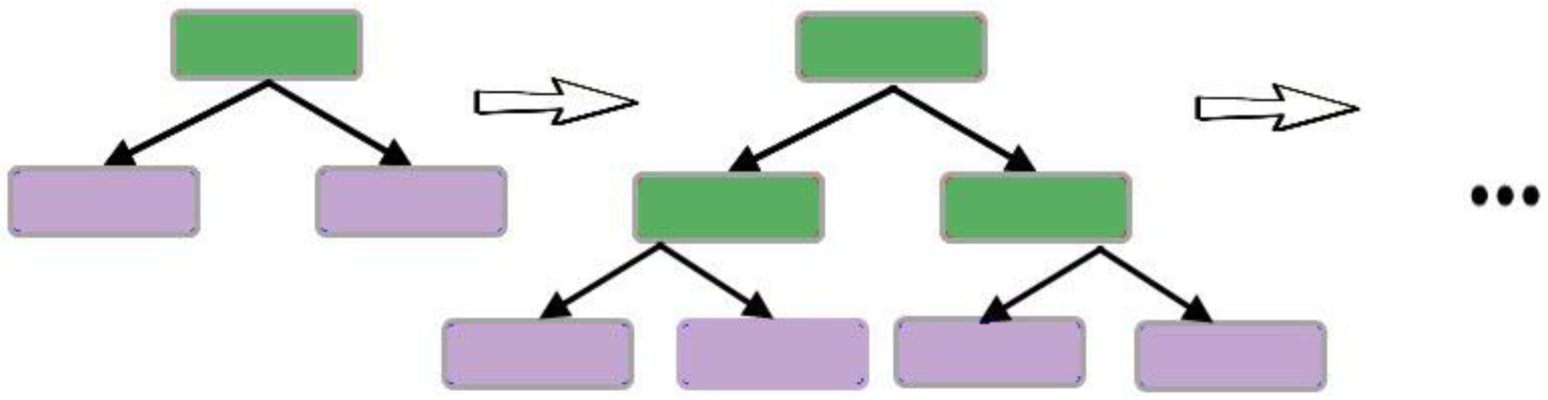
2.2. Adaptive Boosting (AdaBoost)

Boosted DTs are also members of the EL family. As the models are built in such methods, they are adapted to minimize the errors of the previous trees [35,36]. AdaBoost is a type of boosted DT and works on the same principle of boosting, meaning that it retrains samples which are difficult to classify [14,37]. As can be seen in Figure 3, the AdaBoost is sequentially growing DTs, which are made by only one node and two leaves, named stump. In other words, the AdaBoost method is a forest of stumps that incorporates all the trees and uses an iterative approach where at each level of prediction, except the first, a weight is assigned to each of the training items [38].

Unlike boosted DTs in which only the incorrectly classified records from DT are passed on to another stump, in AdaBoost both records are allowed to pass. Here, the strategy is that the incorrectly classified samples are assigned a higher weight and easily classified observations are assigned a lower weight, so they will have a higher probability in the next round of prediction. The second stumps is therefore grown on this weighted data. This process is continued for a specific number of iterations to generate subsequent trees. Once the classifiers are trained, for each classifier a weight will be assigned and the final prediction, which is based on weighted majority vote, will be appraised. To gain reasonable results, a more accurate classifier will receive higher weight, so that it will have more effect in the final prediction. The biggest advantage of this method is that the optimum solution is obtained based on the combination of all the trees and not just the final tree.

The main advantages and disadvantages of using AdaBoost method are listed in

Table 3. Advantages and disadvantages of AdaBoost.

Advantages	Disadvantages
Easy to understand and to visualize	Extremely sensitive to noisy data.
Has only a few hyper-parameters that need to be tuned.	Operates poorer than RF and XGBoost when irrelevant features are included.
Relatively robust to overfitting in low noise datasets.	Is not optimized for speed.
Can be used in both regression and classification problems.

.

2.3. Gradient Boosting Machine (GBM)

GBM is a decision tree-based prediction algorithm [39], which gradually, additively and sequentially produces a model in the form of linear combinations of DTs [40]. Understanding of AdaBoost makes it easy to explain GBM because they are established on the same basis. The most important difference between AdaBoost and GBM methods is the way that they control the shortcomings of weak classifiers. As explained in the previous subsection, in AdaBoost the shortcomings are identified by using high-weight data points that are difficult to fit, but in GBM shortcomings are identified by gradients. The methodology summary here is modeling data with simple base classifiers, analyzing errors, focusing on those hard-to-fit data to get them correct and finally giving some weights to each predictor to combine all predictions to achieve a final result. This technique has shown considerable success in dealing with a wide range of applications and [41,42,43], including text classification [44], web searching [45], landslide susceptibility assessment [46], image classification [47], etc. However, gradient boosting may not have acceptable performance for exceptionally noisy data, as this can result in overfitting. The schematic diagram of the GBM classifier is depicted in Figure 4.

The main advantages and disadvantages of using GBM method are listed in

Table 4. Advantages and disadvantages of GBM.

Advantages	Disadvantages
Works great with categorical and numerical values.	Can cause overfitting.
Can be used in both regression and classification problems.	Less interpretable.
	Can be time and memory exhaustive.

.

2.4. Extreme Gradient Boosting (XGBoost)

XGBoost is a gradient tree boosting method developed by Chen and Guestrin in [42], which applies some improvements over regular GBM. Some of the unique features of XGBoost that make it more powerful are regularization (helps to avoid overfitting), tree pruning (uses Maximum Tree Depth (MTD) parameter to specify tree depth at first and prune tree backward instead of pruning on loss criteria, leading to better computation performance), and parallelism (design of block structure for parallel learning to enable faster computation) [25]. Overall, XGBoost uses a DT as a booster, and has demonstrated excellent performance in many classification, regression, and ranking tasks [43]. However, XGBoost has not been widely studied in the RS image classification tasks in conjunction with spectral and spatial features from views such as classification accuracy, computational effectiveness, and crucial parameter influence. The schematic diagram of this method is shown in Figure 5.

The main advantages and disadvantages of using XGBoost method are listed in

Table 5. Advantages and disadvantages of XGBoost.

Advantages	Disadvantages
Supports parallel processing to be much faster than GBM.	Less interpretable, difficult to visualize and to tune compared to AdaBoost and RF.
Continuous splitting until the MTD specified and then starts pruning the tree backwards to eliminate extra splits beyond which there is no positive gain	It cannot handle categorical values by itself.
Can be used in both regression and classification problems.	Only numerical values are accepted for processing.

.

2.5. Light Gradient Boosting Machine (LightGBM)

The LightGBM algorithm is a gradient boosting framework proposed based on the series of DTs [48]. LightGBM algorithm can effectively reduce the amount of computation while ensuring good accuracy [22,39,48]. An essential difference of the LightGBM framework from other decision-tree-based EL methods is related to the tree growth procedure. Unlike the other methods, which grow trees level-wise (i.e., grows the tree horizontally), the LightGBM algorithm grows trees leaf-wise (i.e., grows tree vertically (see Figure 6)), which leads to an increase in the complexity of its structure [49]. Although the implementation of XGBoost and LightGBM are relatively similar, the LightGBM method is upgraded over the XGBoost in terms of training speed and the size of the data set it can handle. However, improving the classification performance and achieving reliable results in both approaches require extensive parameter tuning compared to other methods like RF.

The main advantages and disadvantages of using LightGBM method are listed in

Table 6. Advantages and disadvantages of using LightGBM.

Advantages	Disadvantages
Avoids overfitting.	It is less used than other ensemble learning methods due to less documentation available.
Better accuracy than other boosting methods.
Get better trees with smaller computational cost.
Handle both categorical and continuous values.
Outperforms XGBoost in terms of computational speed and memory consumptions.
Speeds up the training process of conventional GBM.
Parallel learning supported.

.

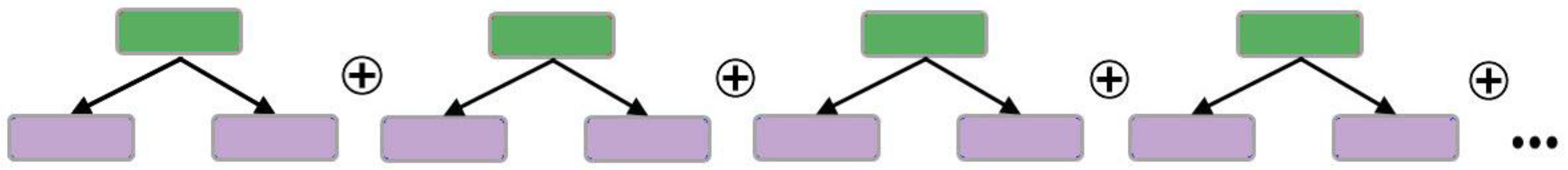
2.6. Random Forest (RF)

RF is a robust EL method consisting of several DT classifiers to overcome the limitations of a single classifier in obtaining the optimal solution (e.g., DT) [50,51,52]. Therefore, an RF algorithm addresses this limitation by incorporating many trees rather than a single tree and uses the majority vote technique to assign a final class label (Figure 7). This idea is further expanded to resolve the issues regarding the handling of the high number of variables in the model. Indeed, the training of each tree in the model is restricted to its self-randomly generated subset of the training data and just employs a subset of that tree’s variables. Although the combination of reduced training data and reduced number of variables decreases the performance of each individual tree, yet there is a smaller correlation between trees and this makes the ensemble as a whole more reliable. Since there are multiple classifiers in the RF algorithm, it is not required to prune the individual trees [50].

The main advantages and disadvantages of using RF method are listed in

Table 7. Advantages and disadvantages of RF.

Advantages	Disadvantages
Handling overfitting and helps to improve the accuracy.	May change considerably by a small change in the data.
Flexible to both classification and regression problems.	Computations may go far more complex.
Handles both categorical and continuous values.	Not easily interpretable.
The power of handle large data sets with higher dimensionality.	Only numerical values are accepted for processing.

.

3. Remote Sensing Datasets

This paper uses three real-world benchmark datasets collected from different types of sensors, including multispectral, hyperspectral, and PolSAR data sets. These data are commonly used in the RS community to evaluate and analyze the performance of state-of-the-art ML and deep learning tools.

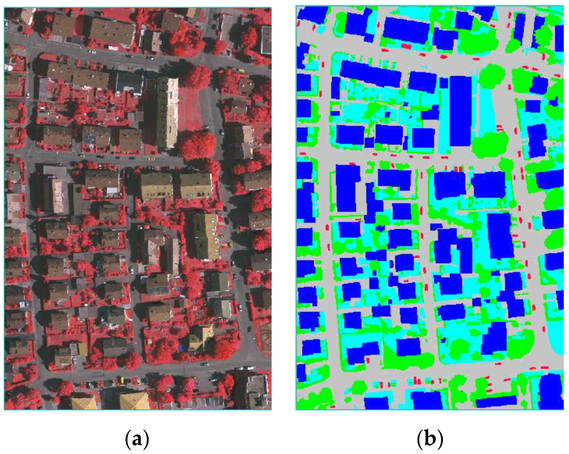
3.1. ISPRS Vaihingen Dataset

This high-resolution multispectral image is a benchmark dataset of the International Society for Photogrammetry and Remote Sensing (ISPRS) 2D semantic labeling challenge in Vaihingen [53]. Vaihingen, Germany is a relatively small village with many detached buildings and small multi-story buildings. The dataset consists of a true ortho-photo with three bands (IRRG: Infrared, Red, and Green), and covers an area of 2006 × 3007 pixels at a GSD (Ground Surface Distance) of about 9 cm. There are five labeled land-cover classes in this dataset: impervious surface, building, low vegetation, tree, and car (listed in

Table 8. The population of samples in the Vaihingen dataset.

#	Class	Samples	Color Code
1	Impervious surfaces	2,059,368
2	Building	1,632,260
3	Low vegetation	1,157,157
4	Tree	1,127,394
5	Car	55,863

). This dataset was acquired using an Intergraph/ZI DMC (Digital Mapping Camera) by the RWE Power company [54]. The study image and its corresponding ground-truth image are shown in Figure 8.

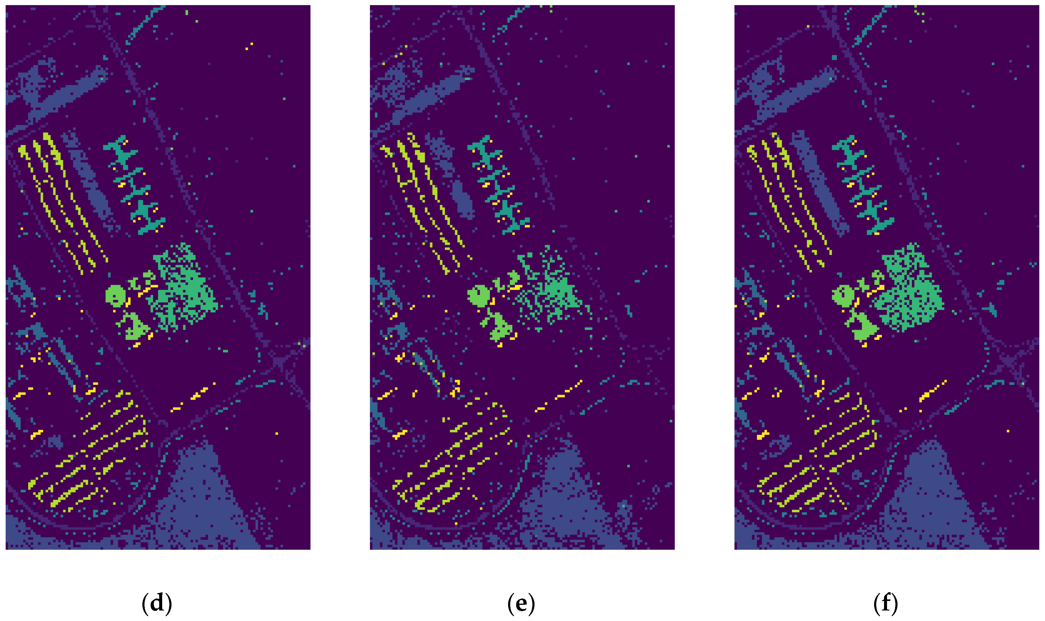
3.2. Pavia University Scene

The second dataset is a hyperspectral image captured by the reflective optics system imaging spectrometer (ROSIS-3) with a GSD of 1.3 meters and 103 spectral bands over Pavia University’s campus in the north of Italy. This scene covers an area of 610 × 340 pixels, including nine land-cover classes. They comprise various urban materials (as listed in

Table 9. Distribution of samples for the Pavia University dataset.

#	Class	Samples	Color Code
1	Asphalt	6631
2	Meadows	18,649
3	Gravel	2099
4	Trees	3064
5	Painted metal sheets	1345
6	Bare Soil	5029
7	Bitumen	1330
8	Self-Blocking Bricks	3682
9	Shadows	947

). The ground truth map of this data covers 50% of the whole surface [55,56]. A false-color composite image (using spectral bands 10, 27, and 46 as R-G-B) and the corresponding ground truth are shown in Figure 9.

3.3. San Francisco Bay SAR Data

Over the past decade, the fully PolSAR C-band data of San Francisco’s bay area has been one of the most employed datasets in the SAR-RS community for polarimetry analysis and classification research. These data cover both northern and southern San Francisco bay with 1380 × 1800 pixels, with a GSD of 8 m collected by RADARSAT-2 on 2 April 2008. It provides a good coverage of both natural (e.g., water and vegetation) and human-made land-covers (e.g., high-density and low-density developed areas) [57]. The Pauli-coded pseudo-color image and the ground truth map of this dataset are shown in Figure 10. The ground truth map represents five land-cover classes listed in

Table 10. Distribution of samples for the San Francisco dataset.

#	Class	Samples	Color Code
1	Water	852,078
2	Vegetation	237,237
3	High-Density Urban	351,181
4	Low-Density Urban	282,975
5	Developed	80,616

.

4. Experiments and Results

4.1. User-Set Parameters

Most ML algorithms have many user-defined parameters that affect classification performance. In

Table 11. Parameter Configuration of algorithms.

Algorithm	Most Important User-Defined Parameters	Example References
DT	maximum tree depth ([0, ∞])	[33,58]
	minimum sample split ([0, ∞])
	minimum sample split ([0, ∞])
	minimum number of samples at a leaf node
AdaBoost	learning rate ([0, 1])	[35]
	number of boosted trees ([0, ∞])
GBM	maximum tree depth ([0, ∞])	[59]
	number of gradient boosted trees
	minimum sample split ([0, ∞])
	learning rate ([0, 1])
XGBoost	maximum tree depth ([0, ∞])	[43]
	number of gradient boosted trees ([0, ∞])
	minimum sample split ([0, ∞])
	learning rate ([0, 1])
LightGBM	maximum tree depth ([0, ∞])	[22,24]
	number of boosted trees ([0, ∞])
	learning rate ([0, 1])
RF	number of decision trees ([0, ∞])	[18,50]
	maximum tree depth ([0, ∞])
	number of variables in each node split
	minimum number of samples at a leaf node
	minimum sample split ([0, ∞])

, there is a list of some of the main parameters according to their function across different models. In this study, we will cover and tune only the important ones, which are listed below. Although the default values are often used for user-set parameters, empirical testing is needed to determine the optimum values for these parameters and thus, make ensure that the best achievable classification result has been obtained. Parameters like Number of Base Classifiers (NBCs), Learning Rate (LR), and MTD, etc. could be optimally selected through validation techniques like k-fold cross-validation. To this end, ‘GridSearchCV’ is set to create a grid search hyper-parameter tuner on the training set.

Some algorithms are particularly interesting because they require few user-defined parameters. For example, the AdaBoost implementation of boosted DT only requires the NBCs in the ensemble and the LR parameter that shrinks each classifier’s contribution. In this study, however, the hyper-parameter optimization experiments for each method are performed based on two user-defined parameters. In other words, we optimize each model via the tuning of two parameters: DT (MTD and Minimum Sample Split (MSS)), AdaBoost (NBCs and LR), GBM (MTD and NBCs), XGBoost (MTD and NBCs), LighGBM (MTD and NBCs), and RF (MTD and NBCs).

The most critical hyper-parameters of six tree-based methods are presented in Table 11. The range of values and the optimal value chosen for each of the parameters are given in the following subsection.

4.1.1. Hyper-Parameter Tuning for Multispectral Data

To provide a comparative analysis of the contribution of inputs/parameters, the mean test accuracy score (MTA) was measured and visualized by plotting the relations of each method’s parameters. The MTA describes the mean accuracy of scores accumulated when predicting the test dataset and is used to rank the competing parameter combinations. For the DT method (Figure 11a), on the ordinate is the MTA of a range of input values calculated for Minimum Sample Split (MSS) while the horizontal axis represents the MTD in the ensemble. As can be seen, by increasing the minimum number of samples, the classifier’s accuracy increases while the MTD is less than 100. On the other hand, the classifier’s accuracy for any given values for the MSS parameter (in this case, 2, 5, 8, and 10) is constant, as the MTD is higher than 100. For the DT method, it makes sense to choose 10 and 100 as the optimum values for MSS and MTD parameters, respectively.

For the AdaBoost method (Figure 11b), on the ordinate is the MTA of a range of input values for LR (i.e., 0.1, 0.3, 0.5, 0.7, and 1) obtained, while on the horizontal axis is the NBCs (i.e., 10, 25, 80 and 100) in the ensemble. Unlike other plots in Figure 11, various tuning parameters substantially affect the AdaBoost algorithm’s accuracy. As shown in Figure 11b, the AdaBoost method has a high accuracy when the LR is set to 1. Moreover, the classification accuracy is almost constant for all input values of the LR while the NBCs is higher than 80. Therefore, from the accuracy and processing time viewpoint, the optimum values for the NBCs and the LR are 80 and 1, respectively, using the AdaBoost method.

To analyze the parameter tuning for GBM, XGBoost, LightGBM, and RF methods, the NBCs and the MTD have been chosen as the most critical parameters in the accuracy of classification results. In Figure 11c–f, on the ordinate is the MTA of a range of input values for MTD (i.e., 10, 20, 30, 40, and 50) measured, while on the horizontal axis is the NBCs in the ensemble. No significant fluctuation in the GBM method’s graphs was observed when different hyper-parameters were set (see Figure 11c). The GBM is a time-consuming method; therefore, the best tuning values for the NBCs and MTD are both 30. In Figure 11d, MTD showed a negative correlation with the accuracy. Overall, the XGBoost method (with MTD = 20 and NBCs = 30) has the best performance.

The smooth trend of the LightGBM method’s graphs illustrates that setting different hyper-parameters does not highly affect classification accuracy. Based on the results, the LightGBM method achieves a high accuracy when the NBCs and MTD are set to 80 and 20, respectively. Note that to decrease the computational cost, setting the NBCs to 50 with a MTD of 10 can also produce acceptable results.

Assessment of the RF classifier’s results shows that increasing of the MTD may cause an increase in computational cost without a positive effect on the accuracy. Figure 11f illustrates that the optimum tuning values for the MTD and the NBCs parameters in the RF method are 20 and 80, respectively.

4.1.2. Hyper-Parameter Tuning for Hyperspectral Data

Changes in the DT method’s input variables do not alter the accuracy when the MTD is set to a value higher than 100. The results of this method, however, reach a high accuracy when the MSS = 8 and MTD = 200. It is interesting to see that this method has a similar trend in both multispectral and hyperspectral datasets.

According to Figure 12b, tuned parameters significantly affect the AdaBoost technique’s accuracy. A similar function was performed in the multispectral dataset too. Yet, increases in the LR value lead to increased accuracy, but increases in the NBCs do not positively affect classification results. As shown in Figure 12b, the best values for the mentioned tuning parameters are 1 and 25, respectively.

According to Figure 12c, the MTD values greater than 30 have degraded the classification results of the GBM method; then, the value of 30 is the optimum MTD. Moreover, for the NBCs higher than 25, the classification accuracy decreases; therefore, the optimum value for NBCs is 25. The XGBoost algorithm also follows a similar trend in multispectral and hyperspectral datasets (see Figure 12d). On the whole, this method with MTD and the NBCs equal to 30 and 50, respectively, had the best performance.

The LightGBM and RF methods by hyperspectral data do not follow the trends when multispectral data have been utilized. Here, the NBCs and MTD do not have a predictable relationship in the LightGBM method. An excessive increase in these two parameters adversely affects classification results (see Figure 12e). According to Figure 12f, the RF method does not have good results for a MTD of 10. When the MTD is higher than 10, the accuracy is almost constant for any given input values of the NBCs. However, the best classification results for the RF method are attained when the NBCs = 250 and MTD = 50.

4.1.3. Hyper-Parameter Tuning for PolSAR Data

Based on Figure 13a, for the San Francisco dataset, the high value of MSS decreases the accuracy of the DT method when the MTD is lower than 150. In addition, for any given input values of the MSS parameter (i.e., 2, 5, 8, 10) when MTD is greater than 150, the classification result is constant. Therefore, the optimum tuning values for MSS and MTD, are 5 and 150, respectively.

Like AdaBoost’s performance for multispectral and hyperspectral datasets, it also has a high dependency on input tuning parameters by PolSAR data. In other words, by increasing the NBCs and LR values, the accuracy increases. The AdaBoost method’s best results were obtained when the NBCs and LR were set to 80 and 0.8, respectively (Figure 13b).

Figure 13c,d show that variation in tuning parameters (i.e., NBCs and MTD) does not alter the accuracy of classification results using GBM and XGBoost algorithms. However, high accuracy for these two methods is achieved when the input variables for GBM and XGBoost are set to (NBCs = 80, MTD = 30) and (NBCs = 50, MTD = 30), respectively.

As illustrated in Figure 13e, there are high variations in the results of the LightGBM method using different input values for the NBCs and MTD parameters. High accuracy is acquired when these parameters are set to 100 and 30, respectively. In addition, the results of the RF approach are also highly dependent on input values. As depicted in Figure 13e, the optimum tuning values for these parameters are NBCs = 150, MTD = 20.

4.2. Classification Results

In this section, the experimental results will be illustrated and the qualitative and quantitative analysis of classification methods will be discussed.

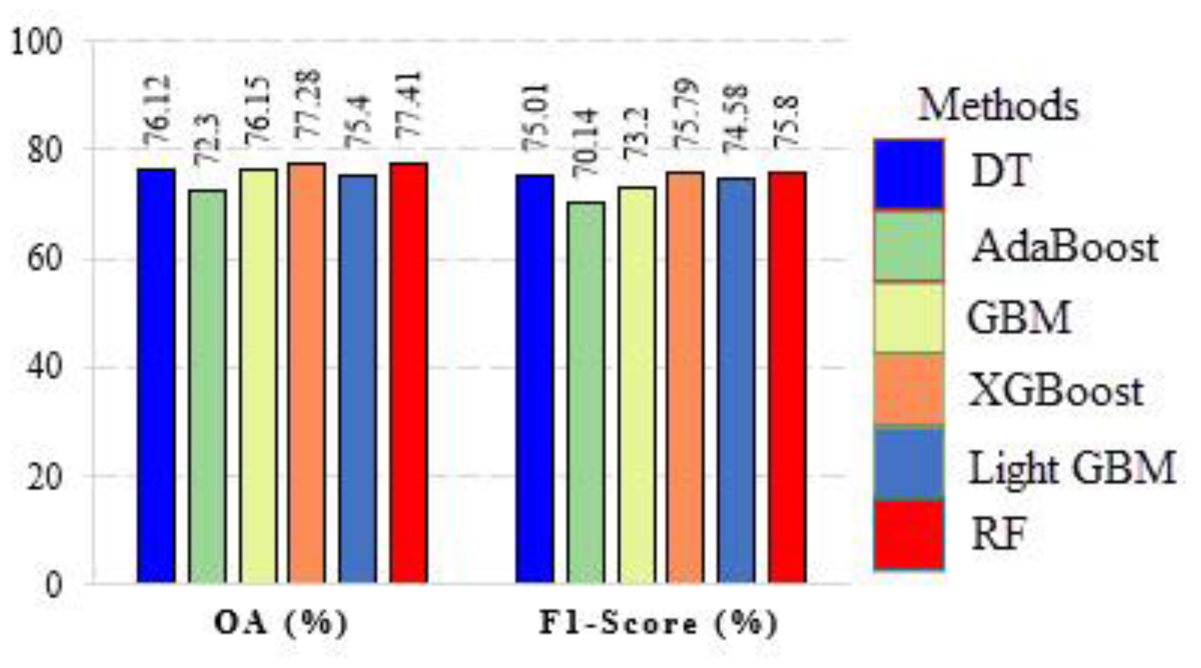
4.2.1. Land-Cover Mapping from Multispectral Data

The classification results of the six implemented ML algorithms using the ISPRS Vaihingen multispectral dataset are demonstrated in Figure 14.

From the quantitative viewpoint, we made a numerical evaluation of classification results. Numerous metrics have been introduced in the literature to evaluate the quality and accuracy of different RS methods. In this paper, the classification methods’ results were assessed by the overall accuracy (OA) and F1-Score (the reader is referred to [60] for more information regarding these metrics). According to Figure 14 and Figure 15, the comparison of classification results demonstrates reliable performances for the RF, XGBoost, and DT classifiers using the multispectral data.

4.2.2. Classification Results of Hyperspectral Data

The classification maps obtained from the six discussed approaches using the Pavia University hyperspectral dataset are illustrated in Figure 16.

From a visual inspection of results in Figure 16, an initial qualitative conclusion can be obtained about the most effective classification algorithms for the Pavia University dataset. Considering the visual assessment of the resulting outputs, the LightGBM and XGBoost models seem to be more effective than other types of approaches in classifying the objects in the scene. The numerical evaluation in Figure 17 supports this conclusion.

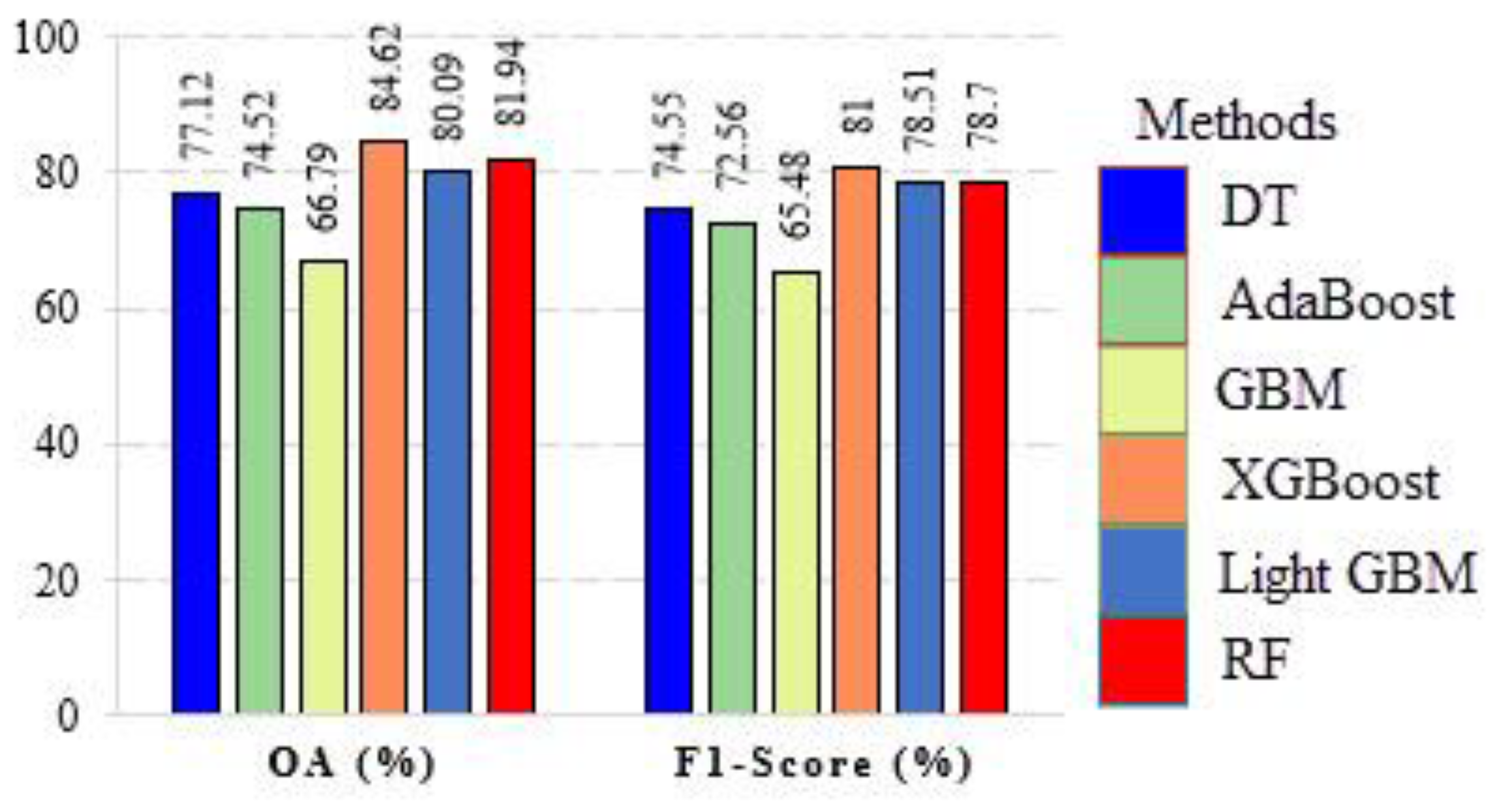
4.2.3. Classification Results of PolSAR Dataset

The classification results for the six implemented ML algorithms using the San Francisco PolSAR dataset are shown in Figure 18.

After the initial visualization, a numerical assessment was performed on the classification maps. As presented in Figure 19, the XGBoost, RF, and LightGBM provided high accuracy; thus, similar to the visual analysis, the classified maps’ numerical evaluation endorsed the effectiveness of these methods.

4.2.4. The Final Summary of Classification Results

Table 12. Comparison between the performance of different methods on the classification of multispectral, hyperspectral, and PolSAR datasets.

Datasets	Metrics	Methods
		DT	AdaBoost	GBM	XGBoost	LightGBM	RF
Multispectral	OA	76.12%	72.3%	76.15%	77.28%	75.4%	77.41%
	F1-Score	75.01%	70.14%	73.2%	75.79%	74.58%	75.8%
Hyperspectral	OA	80.51%	78.29%	83.84%	85.94%	86.34%	85.52%
	F1-Score	79%	72.8%	82.21%	84.48%	83.01%	83.44%
PolSAR	OA	77.12%	74.52%	66.79%	84.62%	80.09%	81.94%
	F1-Score	74.55%	72.56%	65.48%	81%	78.51%	78.7%

gives the summary of different results obtained for each dataset using the six ML methods. Based on this table, the classification of multispectral data with the RF and XGBoost methods achieved OA of 77.41% and 77.28%, respectively, which are the highest accuracies compared to the accuracy of other methods. Moreover, the LightGBM and XGBoost methods using hyperspectral data with OA of 86.34% and 85.94%, respectively, and XGBoost and RF algorithms using PolSAR data with the OA of 84.62% and 81.94%, respectively, produced the higher classification accuracies compared to other ML techniques. In this paper, in terms of the pixel-based classification, the XGBoost method produced better results than the other methods investigated and has a high potential in the classification of different RS data types.

5. Conclusions

In this study, six well-known EL methods, namely AdaBoost, GBM, XGBoost, LightGBM, and RF were compared in their classification of multispectral, hyperspectral, and PolSAR datasets. The performance comparison was based on both hyper-parameter tuning and model accuracy. According to Table 12, analyzing the final results can be examined from two viewpoints: (1) from the methodology viewpoint: since the XGBoost and LightGMB methods are the improved versions of EL algorithms, in the most cases in the current study, they provided the best results; and (2) from the dataset viewpoint: it is interesting to see that all of the techniques produce higher accuracy when dealing with the hyperspectral dataset. Such a result proves that EL algorithms can show a better performance when a high number of features are fed into their models.

Overall, our experimental results showed that the LightGBM, XGBoost, and RF methods were superior to the other techniques in classifying various RS data. However, finding the most suitable parameters for these methods is a challenging and time-consuming process. The input parameters’ optimum values may vary depending on the size of the input dataset and the number/complexity of the class types in the scene. Consequently, setting the appropriate parameters is an important step and affects the classification results.

References

1. Aredehey, G.; Mezgebu, A.; Girma, A. Land-Use Land-Cover Classification Analysis of Giba Catchment Using Hyper Temporal MODIS NDVI Satellite Images. Int. J. Remote Sens. 2018, 39, 810–821. [Google Scholar] [CrossRef]
2. Xia, M.; Tian, N.; Zhang, Y.; Xu, Y.; Zhang, X. Dilated Multi-Scale Cascade Forest for Satellite Image Classification. Int. J. Remote Sens. 2020, 41, 7779–7800. [Google Scholar] [CrossRef]
3. Briem, G.J.; Benediktsson, J.A.; Sveinsson, J.R. Boosting, Bagging, and Consensus Based Classification of Multisource Remote Sensing Data. In Proceedings of the Multiple Classifier Systems; Kittler, J., Roli, F., Eds.; Springer: Berlin/Heidelberg, Germany, 2001; pp. 279–288. [Google Scholar]
4. Jamshidpour, N.; Safari, A.; Homayouni, S. Spectral–Spatial Semisupervised Hyperspectral Classification Using Adaptive Neighborhood. IEEE J. Sel. Top. Appl. Earth Obs. Remote Sens. 2017, 10, 4183–4197. [Google Scholar] [CrossRef]
5. Halder, A.; Ghosh, A.; Ghosh, S. Supervised and Unsupervised Landuse Map Generation from Remotely Sensed Images Using Ant Based Systems. Appl. Soft Comput. 2011, 11, 5770–5781. [Google Scholar] [CrossRef]
6. Chen, Y.; Dou, P.; Yang, X. Improving Land Use/Cover Classification with a Multiple Classifier System Using AdaBoost Integration Technique. Remote Sens. 2017, 9, 1055. [Google Scholar] [CrossRef] [Green Version]
7. Maulik, U.; Chakraborty, D. A Robust Multiple Classifier System for Pixel Classification of Remote Sensing Images. Fundam. Inform. 2010, 101, 286–304. [Google Scholar] [CrossRef]
8. Nowakowski, A. Remote Sensing Data Binary Classification Using Boosting with Simple Classifiers. Acta Geophys. 2015, 63, 1447–1462. [Google Scholar] [CrossRef] [Green Version]
9. Kavzoglu, T.; Colkesen, I.; Yomralioglu, T. Object-Based Classification with Rotation Forest Ensemble Learning Algorithm Using Very-High-Resolution WorldView-2 Image. Remote Sens. Lett. 2015, 6, 834–843. [Google Scholar] [CrossRef]
10. Rokach, L. Ensemble Methods for Classifiers. In Data Mining and Knowledge Discovery Handbook; Maimon, O., Rokach, L., Eds.; Springer US: Boston, MA, USA, 2005; pp. 957–980. ISBN 978-0-387-25465-4. [Google Scholar]
11. Dietterich, T.G. An Experimental Comparison of Three Methods for Constructing Ensembles of Decision Trees: Bagging, Boosting, and Randomization. Mach. Learn. 2000, 40, 139–157. [Google Scholar] [CrossRef]
12. Miao, X.; Heaton, J.S.; Zheng, S.; Charlet, D.A.; Liu, H. Applying Tree-Based Ensemble Algorithms to the Classification of Ecological Zones Using Multi-Temporal Multi-Source Remote-Sensing Data. Int. J. Remote Sens. 2012, 33, 1823–1849. [Google Scholar] [CrossRef]
13. Halmy, M.W.A.; Gessler, P.E. The Application of Ensemble Techniques for Land-Cover Classification in Arid Lands. Int. J. Remote Sens. 2015, 36, 5613–5636. [Google Scholar] [CrossRef]
14. Briem, G.J.; Benediktsson, J.A.; Sveinsson, J.R. Multiple Classifiers Applied to Multisource Remote Sensing Data. IEEE Trans. Geosci. Remote Sens. 2002, 40, 2291–2299. [Google Scholar] [CrossRef] [Green Version]
15. Breiman, L. Bagging Predictors. Mach. Learn. 1996, 24, 123–140. [Google Scholar] [CrossRef] [Green Version]
16. Benediktsson, J.A.; Chanussot, J.; Fauvel, M. Multiple Classifier Systems in Remote Sensing: From Basics to Recent Developments. In Proceedings of the Multiple Classifier Systems; Haindl, M., Kittler, J., Roli, F., Eds.; Springer: Berlin/Heidelberg, Germany, 2007; pp. 501–512. [Google Scholar]
17. Pal, M. Ensemble Learning with Decision Tree for Remote Sensing Classification. Int. J. Comput. Inf. Eng. 2007, 1, 3852–3854. [Google Scholar]
18. Mahdianpari, M.; Jafarzadeh, H.; Granger, J.E.; Mohammadimanesh, F.; Brisco, B.; Salehi, B.; Homayouni, S.; Weng, Q. A Large-Scale Change Monitoring of Wetlands Using Time Series Landsat Imagery on Google Earth Engine: A Case Study in Newfoundland. GISci. Remote Sens. 2020, 57, 1102–1124. [Google Scholar] [CrossRef]
19. Georganos, S.; Grippa, T.; Vanhuysse, S.; Lennert, M.; Shimoni, M.; Kalogirou, S.; Wolff, E. Less Is More: Optimizing Classification Performance through Feature Selection in a Very-High-Resolution Remote Sensing Object-Based Urban Application. GISci. Remote Sens. 2018, 55, 221–242. [Google Scholar] [CrossRef]
20. Ustuner, M.; Balik Sanli, F. Polarimetric Target Decompositions and Light Gradient Boosting Machine for Crop Classification: A Comparative Evaluation. ISPRS Int. J. Geo-Inf. 2019, 8, 97. [Google Scholar] [CrossRef] [Green Version]
21. Abdi, A.M. Land Cover and Land Use Classification Performance of Machine Learning Algorithms in a Boreal Landscape Using Sentinel-2 Data. GISci. Remote Sens. 2020, 57, 1–20. [Google Scholar] [CrossRef] [Green Version]
22. Shi, X.; Cheng, Y.; Xue, D. Classification Algorithm of Urban Point Cloud Data Based on LightGBM. IOP Conf. Ser. Mater. Sci. Eng. 2019, 631, 052041. [Google Scholar] [CrossRef]
23. Jiang, H.; Li, D.; Jing, W.; Xu, J.; Huang, J.; Yang, J.; Chen, S. Early Season Mapping of Sugarcane by Applying Machine Learning Algorithms to Sentinel-1A/2 Time Series Data: A Case Study in Zhanjiang City, China. Remote Sens. 2019, 11, 861. [Google Scholar] [CrossRef] [Green Version]
24. Krishna Moorthy, S.M.; Calders, K.; Vicari, M.B.; Verbeeck, H. Improved Supervised Learning-Based Approach for Leaf and Wood Classification from LiDAR Point Clouds of Forests. IEEE Trans. Geosci. Remote Sens. 2020, 58, 3057–3070. [Google Scholar] [CrossRef] [Green Version]
25. Zhong, L.; Hu, L.; Zhou, H. Deep Learning Based Multi-Temporal Crop Classification. Remote Sens. Environ. 2019, 221, 430–443. [Google Scholar] [CrossRef]
26. Saini, R.; Ghosh, S.K. Crop Classification in a Heterogeneous Agricultural Environment Using Ensemble Classifiers and Single-Date Sentinel-2A Imagery. Geocarto Int. 2019, 1–19. [Google Scholar] [CrossRef]
27. Dey, S.; Mandal, D.; Robertson, L.D.; Banerjee, B.; Kumar, V.; McNairn, H.; Bhattacharya, A.; Rao, Y.S. In-Season Crop Classification Using Elements of the Kennaugh Matrix Derived from Polarimetric RADARSAT-2 SAR Data. Int. J. Appl. Earth Obs. Geoinf. 2020, 88, 102059. [Google Scholar] [CrossRef]
28. Gašparović, M.; Dobrinić, D. Comparative Assessment of Machine Learning Methods for Urban Vegetation Mapping Using Multitemporal Sentinel-1 Imagery. Remote Sens. 2020, 12, 1952. [Google Scholar] [CrossRef]
29. Chan, J.C.W.; Huang, C.; Defries, R. Enhanced Algorithm Performance for Land Cover Classification from Remotely Sensed Data Using Bagging and Boosting. IEEE Trans. Geosci. Remote Sens. 2001, 39, 693–695. [Google Scholar] [CrossRef]
30. Friedl, M.A.; Brodley, C.E. Decision Tree Classification of Land Cover from Remotely Sensed Data. Remote Sens. Environ. 1997, 61, 399–409. [Google Scholar] [CrossRef]
31. Song, Y.Y.; Ying, L.U. Decision Tree Methods: Applications for Classification and Prediction. Shanghai Arch. Psychiatry 2015, 27, 130–135. [Google Scholar] [CrossRef]
32. Sharma, R.; Ghosh, A.; Joshi, P.K. Decision Tree Approach for Classification of Remotely Sensed Satellite Data Using Open Source Support. J. Earth Syst. Sci. 2013, 122, 1237–1247. [Google Scholar] [CrossRef] [Green Version]
33. Maxwell, A.E.; Warner, T.A.; Fang, F. Implementation of Machine-Learning Classification in Remote Sensing: An Applied Review. Int. J. Remote Sens. 2018, 39, 2784–2817. [Google Scholar] [CrossRef] [Green Version]
34. Pal, M.; Mather, P.M. An Assessment of the Effectiveness of Decision Tree Methods for Land Cover Classification. Remote Sens. Environ. 2003, 86, 554–565. [Google Scholar] [CrossRef]
35. Freund, Y.; Schapire, R.E. Experiments with a New Boosting Algorithm. In Proceedings of the Thirteenth International Conference on International Conference on Machine Learning, Bari, Italy, 3 July 1996; Morgan Kaufmann Publishers Inc.: San Francisco, CA, USA, 1996; pp. 148–156. [Google Scholar]
36. Chan, J.C.-W.; Paelinckx, D. Evaluation of Random Forest and Adaboost Tree-Based Ensemble Classification and Spectral Band Selection for Ecotope Mapping Using Airborne Hyperspectral Imagery. Remote Sens. Environ. 2008, 112, 2999–3011. [Google Scholar] [CrossRef]
37. Freund, Y.; Schapire, R.E. A Decision-Theoretic Generalization of On-Line Learning and an Application to Boosting. J. Comput. Syst. Sci. 1997, 55, 119–139. [Google Scholar] [CrossRef] [Green Version]
38. Dou, P.; Chen, Y. Dynamic Monitoring of Land-Use/Land-Cover Change and Urban Expansion in Shenzhen Using Landsat Imagery from 1988 to 2015. Int. J. Remote Sens. 2017, 38, 5388–5407. [Google Scholar] [CrossRef]
39. Friedman, J.H. Greedy Function Approximation: A Gradient Boosting Machine. Ann. Statist. 2001, 29, 1189–1232. [Google Scholar] [CrossRef]
40. Biau, G.; Cadre, B.; Rouvìère, L. Accelerated Gradient Boosting. arXiv 2018, arXiv:1803.02042. [Google Scholar] [CrossRef] [Green Version]
41. Prioritizing Influential Factors for Freeway Incident Clearance Time Prediction Using the Gradient Boosting Decision Trees Method—IEEE Journals & Magazine. Available online: https://0-ieeexplore-ieee-org.brum.beds.ac.uk/document/7811191 (accessed on 16 January 2021).
42. Chen, T.; Guestrin, C. XGBoost: A Scalable Tree Boosting System. In Proceedings of the 22nd ACM SIGKDD International Conference on Knowledge Discovery and Data Mining; Association for Computing Machinery, New York, NY, USA, 13 August 2016; pp. 785–794. [Google Scholar]
43. Samat, A.; Li, E.; Wang, W.; Liu, S.; Lin, C.; Abuduwaili, J. Meta-XGBoost for Hyperspectral Image Classification Using Extended MSER-Guided Morphological Profiles. Remote Sens. 2020, 12, 1973. [Google Scholar] [CrossRef]
44. Natekin, A.; Knoll, A. Gradient Boosting Machines, a Tutorial. Front. Neurorobot. 2013, 7, 21. [Google Scholar] [CrossRef] [Green Version]
45. Zheng, Z.; Zha, H.; Zhang, T.; Chapelle, O.; Chen, K.; Sun, G. A General Boosting Method and Its Application to Learning Ranking Functions for Web Search. In Proceedings of the Advances in Neural Information Processing Systems 20: Proceedings of the 2007 Conference, Vancouver, BC, Canada, 3–6 December 2007. [Google Scholar]
46. Lombardo, L.; Cama, M.; Conoscenti, C.; Märker, M.; Rotigliano, E. Binary Logistic Regression versus Stochastic Gradient Boosted Decision Trees in Assessing Landslide Susceptibility for Multiple-Occurring Landslide Events: Application to the 2009 Storm Event in Messina (Sicily, Southern Italy). Nat. Hazards 2015, 79, 1621–1648. [Google Scholar] [CrossRef]
47. Li, L.; Wu, Y.; Ye, M. Multi-Class Image Classification Based on Fast Stochastic Gradient Boosting. Informatica 2014, 38, 145–153. [Google Scholar]
48. Ke, G.; Meng, Q.; Finley, T.; Wang, T.; Chen, W.; Ma, W.; Ye, Q.; Liu, T.-Y. LightGBM: A Highly Efficient Gradient Boosting Decision Tree. Adv. Neural Inf. Process. Syst. 2017, 30, 3146–3154. [Google Scholar]
49. Machado, M.R.; Karray, S.; Sousa, I.T. de LightGBM: An Effective Decision Tree Gradient Boosting Method to Predict Customer Loyalty in the Finance Industry. In Proceedings of the 2019 14th International Conference on Computer Science Education (ICCSE), Toronto, ON, Canada, 19–21 August 2019; pp. 1111–1116. [Google Scholar]
50. Breiman, L. Random Forests. Mach. Learn. 2001, 45, 5–32. [Google Scholar] [CrossRef] [Green Version]
51. Cutler, D.R.; Edwards, T.C.; Beard, K.H.; Cutler, A.; Hess, K.T.; Gibson, J.; Lawler, J.J. Random Forests for Classification in Ecology. Ecology 2007, 88, 2783–2792. [Google Scholar] [CrossRef]
52. Belgiu, M.; Drăguţ, L. Random Forest in Remote Sensing: A Review of Applications and Future Directions. ISPRS J. Photogramm. Remote Sens. 2016, 114, 24–31. [Google Scholar] [CrossRef]
53. ISPRS International Society For Photogrammetry And Remote Sensing. 2D Semantic Labeling Challenge. Available online: https://www2.isprs.org/commissions/comm2/wg4/benchmark/semantic-labeling/ (accessed on 15 January 2021).
54. Cheng, W.; Yang, W.; Wang, M.; Wang, G.; Chen, J. Context Aggregation Network for Semantic Labeling in Aerial Images. Remote Sens. 2019, 11, 1158. [Google Scholar] [CrossRef] [Green Version]
55. Audebert, N.; Saux, B.L.; Lefevre, S. Deep Learning for Classification of Hyperspectral Data: A Comparative Review. IEEE Geosci. Remote Sens. Mag. 2019, 7, 159–173. [Google Scholar] [CrossRef] [Green Version]
56. Gao, F.; Wang, Q.; Dong, J.; Xu, Q. Spectral and Spatial Classification of Hyperspectral Images Based on Random Multi-Graphs. Remote Sens. 2018, 10, 1271. [Google Scholar] [CrossRef] [Green Version]
57. Uhlmann, S.; Kiranyaz, S. Integrating Color Features in Polarimetric SAR Image Classification. IEEE Trans. Geosci. Remote Sens. 2014, 52, 2197–2216. [Google Scholar] [CrossRef]
58. Quinlan, J.R. Induction of Decision Trees. Mach. Learn. 1986, 1, 81–106. [Google Scholar] [CrossRef] [Green Version]
59. Zhang, F.; Du, B.; Zhang, L. Scene Classification via a Gradient Boosting Random Convolutional Network Framework. IEEE Trans. Geosci. Remote Sens. 2016, 54, 1793–1802. [Google Scholar] [CrossRef]
60. Jafarzadeh, H.; Hasanlou, M. An Unsupervised Binary and Multiple Change Detection Approach for Hyperspectral Imagery Based on Spectral Unmixing. IEEE J. Sel. Top. Appl. Earth Obs. Remote Sens. 2019, 12, 4888–4906. [Google Scholar] [CrossRef]
61. Cramer, M. The DGPF-Test on Digital Airborne Camera Evaluation Overview and Test Design. Photogramm. Fernerkund. Geoinf. 2010, 73–82. [Google Scholar] [CrossRef] [PubMed]
Figure 1. A general structure of an EL approach.
Remotesensing 13 04405 g001
Figure 2. Schematic diagram of the DT classifier (nodes and leaves are colored green and purple, respectively).
Remotesensing 13 04405 g002
Figure 3. Schematic diagram of AdaBoost classifier.
Remotesensing 13 04405 g003
Figure 4. Schematic diagram of GBM classifier.
Remotesensing 13 04405 g004
Figure 5. Schematic diagram of XGBoost classifier.
Remotesensing 13 04405 g005
Figure 6. Schematic diagram of LightGBM classifier.
Remotesensing 13 04405 g006
Figure 7. A schematic diagram of the RF classifier.
Remotesensing 13 04405 g007
Figure 8. A scene sample of the Vaihingen dataset and the ground-truth map. (a) True color image; and (b) GT.
Remotesensing 13 04405 g008
Figure 9. Pavia University scene dataset and the ground-truth map. (a) False color image; and (b) GT.
Remotesensing 13 04405 g009
Figure 10. San Francisco PolSAR dataset and its corresponding ground truth data. (a) Pauli color coded image; and (b) GT.
Remotesensing 13 04405 g010
Figure 11. Hyper-parameter analysis of different EL methods using ISPRS Vaihingen data. (a) DT, (b) AdaBoost, (c) GBM, (d) XGBoost, (e) LightGBM, and (f) RF.
Remotesensing 13 04405 g011aRemotesensing 13 04405 g011b
Figure 12. Hyper-parameter analysis of different EL methods using Pavia hyperspectral data. (a) DT, (b) AdaBoost, (c) GBM, (d) XGBoost, (e) LightGBM, and (f) RF.
Remotesensing 13 04405 g012
Figure 13. Hyper-parameter analysis of different EL methods using San Francisco PolSAR dataset. (a) DT, (b) AdaBoost, (c) GBM, (d) XGBoost, (e) LightGBM, and (f) RF.
Remotesensing 13 04405 g013aRemotesensing 13 04405 g013b
Figure 14. Classification results for ISPRS Vaihingen dataset. (a) DT, (b) AdaBoost, (c) GBM, (d) XGBoost, (e) Light GBM, and (f) RF.
Remotesensing 13 04405 g014
Figure 15. Numerical evaluation of EL techniques in the classification of the multispectral dataset.
Remotesensing 13 04405 g015
Figure 16. Classification results for Pavia University data. (a) DT, (b) AdaBoost, (c) GBM, (d) XGBoost, (e) Light GBM, and (f) RF.
Remotesensing 13 04405 g016aRemotesensing 13 04405 g016b
Figure 17. Numerical evaluation of EL techniques in the classification of the hyperspectral dataset.
Remotesensing 13 04405 g017
Figure 18. Classification results for San Francisco data. (a) DT, (b) AdaBoost, (c) GBM, (d) XGBoost, (e) Light GBM, and (f) RF.
Remotesensing 13 04405 g018
Figure 19. Numerical evaluation of EL techniques in the classification of San Francisco data.
Remotesensing 13 04405 g019