The Effect of Spatial Resolution and Temporal Sampling Schemes on the Measurement Error for a Moon-Based Earth Radiation Observatory

Abstract

The Moon-Based Earth Radiation Observatory (MERO) is a new platform, which is expected to advance current Earth radiation budget (ERB) research with better observations. For the instrument design of a MERO system, ascertaining the spatial resolution and sampling scheme is important. However, current knowledge about this is still limited. Here we proposed a simulation method for the MERO-measured Earth top of atmosphere (TOA) outgoing shortwave radiation (OSR) and outgoing longwave radiation (OLR) fluxes and constructed the “true” Earth TOA OSR and OLR fluxes based on the Clouds and Earth’s Radiant Energy System (CERES) data. Then we used them to reveal the effects of spatial resolution and temporal scheme (sampling interval and the temporal sampling sequence) on the measurement error of a MERO. Our results indicate that the spatial sampling error in the unit of percentage reduces linearly as the spatial resolution varies from 1000 km to 100 km; the rate is 2.5%/100 km for the Earth TOA OSR flux, which is higher than that (1%/100 km) of the TOA OLR flux. Besides, this rate becomes larger when the spatial resolution is finer than 40 km. It is also demonstrated that a sampling temporal sequence of starting time of 64 min with a sampling interval of 90 min is the optimal sampling scheme that results in the least temporal sampling error for the MERO system with a 40 km spatial resolution, note that this conclusion depends on the temporal resolution and quality of the data used to construct the “true” Earth TOA OSR and OLR fluxes. The proposed method and derived results in this study could facilitate the ascertainment of the optimal spatial resolution and sampling scheme of a MERO system under certain manufacturing budget and measurement error limit.

1. Introduction

Climate change on Earth is dominated by the budget of the incoming and outgoing radiation [1]. The incoming source is solar radiation, whereas the outgoing one is comprised of two parts: outgoing shortwave radiation (OSR) and outgoing longwave radiation (OLR). Since the 1970s, have been several satellite-based missions that were dedicated to OSR and OLR observations, such as the Earth Radiation Budget Experiment (ERBE) [2], the Clouds and Earth’s Radiant Energy System (CERES) [3,4], the Geostationary Earth Radiation Budget (GERB) [5] and the National Institute of Standards and Technology Advanced Radiometer (NISTAR) onboard the Deep Space Climate Observatory (DSCOVR) [6]. Though these low-Earth-orbit (LEO) and geostationary-Earth-orbit (GEO) satellite missions have indeed strengthened our understanding of the Earth radiation budget (ERB), there are still several limitations, which can be complemented by a Moon-Based Earth Radiation Observatory (MERO). Compared to current LEO and GEO ERB systems, a MERO has several advantages: (1) Global ERB observation needs an artificial satellite constellation; however, different satellites have various orbits, which would result in inconsistency between data produced by these satellites. In comparison, a MERO could produce a long-term ERB record with better consistency. Since the Moon–Earth distance (near 380,000 km) is approximately 100 times larger than the diameter of the Moon (3476 km), the distance between any location on the Moon’s nearside and the Earth’s center varies by less than 5%, and the viewing angle towards Earth (the viewing angle or viewing azimuth angle) differs by less than 2%. This implies that almost all locations on the nearside of the Moon have nearly the same viewing geometry towards Earth. Therefore, MERO missions launched at different times with different landing locations would share a highly similar viewing geometry, producing long-term OSR and OLR observations with good consistency. (2) Current LEO ERB systems could not record the rapid variability of the OLR and OSR of the Earth system due to the limited temporal sampling coverage. In contrast, the temporal sampling coverage of a MERO is far higher than the LEO counterparts. The sampling period of a MERO is approximately 12 h per day for a fixed location on Earth, resulting in about 48 temporal samples per day if the sampling interval is set to 15 min (the GERB sampling interval). It is about 24 times larger than that of a low-orbit satellite ERB instrument. These abundant temporal samples would substantially enhance the quality of the diurnal data produced by the ERB fitting method and could help to reveal the small-temporal-scale variations of the TOA OLR and OSR. (3) Current satellite-based ERB data of the polar regions have several problems. The sun-synchronous-LEO ERB system could cover the high-latitude regions; however, the sampling frequency is limited, Therefore, evident error would emerge when the LEO ERB system is used to capture short-temporal processes during specific periods, such as the melting season [7,8]. Besides, current GEO ERB systems also cannot provide satisfied observations for the polar regions [9]. A MERO could provide better OSR and OLR observations of the Arctic and Antarctic regions to complement these limitations. As illustrated by previous research, a MERO could instantaneously observe more than 45% of the Antarctic or Arctic regions during half of a lunar orbital period (27.3 days) to provide abundant samples for a polar location, the amount of these samples are about 24 times larger than a LEO ERB system [10]. Current and previous space-based ERB mission could not capture the Earth system’s inherent and rapid variability of the OLR and OSR with an accepted accuracy due in part to the limited temporal coverage. Therefore, the Earth radiation imbalance cannot be measured definitively [11].

Recent CubeSat ERB missions, such as radiometer assessment using vertically aligned nanotubes (RAVAN) [12] and ultraviolet and infrared sensors at high quantum efficiency onboard a small satellite (UVSQ-SAT) [13], have the potential to improve the temporal coverage of OLR and OSR observations with a constellation of substantial numbers of low-cost compact satellites. Similarly, a MERO would also provide an opportunity to measure the Earth’s OLR and OSR variations at a small temporal scale. A MERO could continuously observe a certain region 12 h per day on average, thus producing near-real-time TOA OLR and OSR measurement every 15 min under the state of the art (15 min is the sampling interval of the in-orbit GERB). Compared to the CubeSat ERB mission, a MERO could provide a simultaneous half-globe TOA OLR and OSR fluxes at an accepted spatial resolution; such data could help to reveal the regional and global radiation imbalance with accepted accuracy without the bias introduced by the non-simultaneous sampling of spatial and temporal variability of TOA OSR and OLR. The keys to limiting the temporal sampling coverage of the CubeSat mission and MERO are different. For CubeSat ERB missions, the primary factor to restrict the temporal sampling coverage is the number of satellites in the constellation. However, this challenges the maintenance and calibration of the system. Numerous small satellites need an effective constellation exit-and-replacement launch procedure; the calibration and inter-calibration of a constellation with such a small number of satellites are still a technique challenge [14]. For a MERO system, the major limit to the temporal sampling frequency is the state-of-art of the instrument, which is closely related to the detector response time, the thermal noise, the data storage and transmit capacity and other related systematic parameters.

With the progressive implementation of the Chinese lunar exploration program (the Change-E missions), a MERO is likely to be deployed in the near future. A MERO system is designed as a non-scanner multi-pixel spectroradiometer with two bands: 0.2–4 μm for the measurement of the Earth top of atmosphere (TOA) OSR flux and 4–100 μm for the Earth TOA OLR flux. The typical observing scenario of a MERO system is shown in Figure 1. Nearly half of the globe is observed by a MERO sensor simultaneously. A detector unit of the focal plane array (FPA) just focuses on a certain region; OSR/OLR radiation coming from the detector-viewed region (pixel) on the Earth TOA (hollow green rectangle in Figure 1) passes through the MERO optical system, then arrives at the detector unit (solid green rectangle in Figure 1) of the FPA. Thereafter the radiation is transformed to an electrical signal by this detector unit. Subsequently, this electrical signal would be processed by the readout circuit and finally be outputted as the digital number (DN) value. However, there are several disadvantages of the MERO platform. The orbiting of the Moon around Earth would result in inconsistency in the number of samples at different latitudes on Earth. For example, the regions with latitude >70° or <−70° can only be viewed by a MERO over half of the Moon’s orbital period, whereas other regions can be viewed for a whole orbital period. Due to the long Earth–Moon distance, the MERO signal is substantially less powerful than current low Earth orbit (LEO) and geostationary Earth orbit (GEO) satellites, which means that the MERO instrument should have much less noise than current satellite-based instrument to cope with the weak signal. Because of the weak magnetic field of the Moon, there will be a large number of high-energy particles on the Moon, which would affect the operation of the MERO instrument. Therefore, a robust protection system is crucially needed.

As for the instrument design, it is necessary to determine the spatial resolution and temporal sampling scheme (sampling interval and sampling temporal sequence). The spatial resolution represents the smallest detecting area that the remote sensing system could recognize, and the observed physical quantity is averaged within such an area. Therefore, the spatial-dependent variability would be ignored due to this averaging, resulting in certain measurement errors. Increasing spatial resolution would restore more spatial variability of the observed physical quantity, and accordingly, reduce the measurement error. Functions of the measurement error versus the spatial resolution of different remote sensing platforms differ, since the observing geometry features are different and so are the observed physical quantity characteristics. Therefore, it is necessary to evaluate the relationship between the spatial resolution and the measurement error for the MERO system, which could facilitate the determination of spatial resolution. However, current knowledge about this relationship is still limited.

Similarly, the sampling interval represents the time difference that the adjacent samplings have. A shorter sampling interval would result in more samples for a certain period, thus giving a more precise observation. Besides, at a certain sampling interval, the sampling temporal sequence (the time location within the temporal sampling interval from which the observations are made) would also have consequences for the measurement error, since it could affect the final temporal interpolation that derives the continuous data. However, the effects of the sampling interval and sampling temporal sequence on the measurement error of a MERO remain poorly understood.

The objective of this paper is to reveal the influences of spatial resolution and temporal sampling schemes (sampling interval and sampling temporal sequence) on the measurement error, which could facilitate the determination of the optimal spatial resolution and the sampling scheme of the MERO instrument under the specified manufacturing cost limit and accuracy requirement. Section 2 describe the methodology of measurement error computation. Section 3 presents the error-with-spatial-resolution relationship and the temporal-sampling-scheme-induced error over March 2019. Discussion and conclusions are exhibited in Section 4 and Section 5, respectively.

2. Methodology

A MERO mainly measures the TOA OSR and OLR fluxes of the Earth. The configuration of the optimal spatial resolution and sampling scheme (sampling intervals and sampling temporal sequence) is a crucial task in the MERO design process. To facilitate this configuration, we assessed the effects of the spatial resolution and sampling schemes on the measurement error in this study. To derive the measurement error, it is necessary to gain the true TOA OSR and OLR fluxes.

2.1. The True OSR and OLR Fluxes

To quantify the introduced error by certain set of spatial resolution and temporal sampling scheme, here we use the CERES SYN ED4.1A dataset to construct the true OSR and OLR fluxes. Such data is chosen due to its high spatial-temporal resolution (up to 1° longitude × 1° latitude of spatial resolution and hourly temporal resolution) and the acceptable accuracy (uncertainties of OSR and OLR are less than 8 W/m² and 3 W/m², respectively) [15,16].

We utilized the global map of the TOA OLR and OSR fluxes of March 2019 with spatial resolution of 0.1° latitude × 0.1° longitude (10 km at equator) and temporal resolution of 1-min to serve as the true OLR and OSR fluxes. The data of March 2019 is chosen since it can make a good assessment of the measurement error at Earth’s polar regions (both the Arctic and Antarctic regions have 12 h in daytime at March). These 0.1° longtitude × 0.1° latitude-1 min OSR and OLR fluxes maps are derived through two steps: 1. spatially interpolating the 1° longtitude × 1° latitude global TOA OSR and OLR fluxes data from CERES SYN-1 dataset with the cubic spline interpolation; 2. temporally interpolating the data derived from step 1 with a combination of half-sine and linear interpolations. This is due to the fact that both the TOA OSR and OLR fluxes follow a sine/cosine pattern over the daytime and that the OSR stays at 0 W/m² during night (whereas the OLR would keep a linear variation during the night-time) [17]. Figure 2 shows the original hourly CERES SYN flux data (discretized points) and the interpolated TOA OSR and OLR fluxes (solid lines) of a certain place (20° E, 30° S) on Earth. The 1-min true OSR flux is derived by half-sine-interpolation at daytime (0 W/m² at night) (Figure 2a); whereas the 1-min true OLR flux is derived by half-sine interpolation during the day and linear interpolation at night of the hourly data (Figure 2b). Notably, this half-sine fit method performs well over land where there is an evident diurnal cycle of both OSR and OLR fluxes. However, this may not work well over regions where the OSR and OLR diurnal cycle is not obvious, such as ocean. This may introduce certain uncertainty to the results.

2.2. Simulation of MERO-Measured TOA OSR and OLR Fluxes

The measurement error could be derived through the difference between the simulated MERO-measured value and the true value, where the simulated MERO-measured OSR flux (M^OSR) and OLR flux (M^OLR) of a certain pixel could be derived through Equation (1):

$$M^k=\frac{{\displaystyle \sum _{i=1}^N{F}_i{}^k{D}_i{}^{-2}{P}_i{}^k{A}_i\cos v_i\cos {\omega }_i}}{P^k\cos \left(v\right)\cos \left(\omega \right)D^{-2}A} k=\mathrm{OSR} \mathrm{or} \mathrm{OLR}$$

(1)

where the subscript i denote a sub grid point (0.1° longtitude × 0.1° latitude) within the pixel. The relationship between the MERO detector array and the pixel array on Earth TOA is shown in Figure 3. The pixel is the area on Earth TOA, which is viewed by the corresponding detector of a MERO instrument; for example, detector 1 views pixel 1’. Every pixel is discretized into uniformed sub grid points, every sub grid point represents a 0.1° latitude × 0.1° longitude area, e.g., the pixel 8’ in Figure 3. F_i^OSR and F_i^OLR are the true OSR and OLR fluxes of the internal point i respectively, which could be derived from the true OSR and OLR fluxes constructed above by cubic spline interpolation. v_i is the viewing zenith angle of sub grid point i. ω_i denotes the angle between the viewing vector and the Earth’s center viewing vector. D_i is the distance between the MERO and the internal grid point i. v is the viewing zenith angle of the whole pixel, which is set as the viewing zenith angle of the centre internal point of the pixel; ω and D are defined in the same way. A and A_i are the area that the whole pixel and the internal point represent, respectively. v_i, v, ω_i, ω, D_i, D, A and A_i could be derived through the MERO pixel positioning method we proposed based on our previous work [18]; geometries of these parameters are shown in Figure 4. P_i^OSR/P_i^OLR in Equation (1) is the TOA OSR/OLR anisotropic factor of the sub grid point i, which is the ratio of the actual OSR/OLR radiance to the Earth TOA OSR/OLR flux and could be derived by Equation (2):

$$P_i^k=\frac{\pi I_i^k}{F_i^k} k=\mathrm{OSR} \mathrm{or} \mathrm{OLR}$$

(2)

where I_i^OSR and I_i^OLR are the actual OSR and OLR radiances from the sub grid point i of the pixel to the MERO detector, respectively. P_i^OSR could be derived through the CERES angular distribution models (ADMs) [19,20]. The ADMs generate the TOA OSR anisotropic factors according to the OSR scene type. Every OSR scene type corresponds to a certain TOA OSR anisotropic factor by considering the dependence of the TOA OSR anisotropic factor on related parameters. These parameters are shown in

Table 1. Parameters used for TOA OSR scene type construction to derive the TOA OSR anisotropy factors in the CERES angular distribution models.

Surface Type	Cloud Conditions	Cloud or Meteorological Parameters	Angles
land and desert	(a) clear (b) cloudy	cloudy condition: cloud type (liquid water or ice cloud) cloud fraction (5 intervals: 0.1–25%, 25–50%, 50–75%, 75–99.9%, 99.9–100%) optical depth (6 intervals: 0–2.5, 2.5–6, 6–10, 10–18, 18–40, >40)	(a) solar zenith angle (9 intervals: same as for ocean) (b) relative azimuth angle (10 intervals: same as for ocean) (c) viewing zenith angle (9 intervals: same as for ocean)
ocean	(a) clear (b) cloudy	(a) clear condition: wind speed (4 intervals: <3.5, 3.5–5.5, 5.5–7.5, >7.5 m s–1) (b) cloudy conditions: cloud type (liquid water or ice cloud) cloud fraction (12 intervals: 0.1–10%, 10–20%, 20–30%, 30–40%, 40–50%, 50–60%, 60–70%, 70–80%, 80–90%, 90–95%, 95–99.9%, 99.9–100%) optical depth (14 intervals: 0–1, 1–2.5, 2.5–5, 5–7.5, 7.5–10, 10–12.5, 12.5–15, 15–17.5, 17.5–20, 20–25, 25–30, 30–40, 40–50, >50)	(a) solar zenith angle (9 intervals: 0°–90° with step of 10°) (b) relative azimuth angle (10 intervals: 0°–10°, 10°–30°, 30°–50°, 50°–70°, 70°–90°, 90°–110°, 110°–130°, 130°–150°, 150°–170°, 170°–180°) (c) viewing zenith angle (9 intervals: same as the solar zenith angle)
snow	(a) clear (b) cloudy	cloudy condition: cloud fraction (5 intervals: 0.1–25%, 25–50%, 50–75%, 75–99.9%, 99.9–100%) optical depth (2 intervals: ≤10, >10)	(a) solar zenith angle (45 intervals: steps of 2° from 0° to 90°) (b) relative azimuth angle (10 intervals: same as for ocean) (c) viewing zenith angle (9 intervals: same as ocean)

, which includes: (1) the type of the surface beneath the TOA area based on the International Geosphere and Biosphere Program (IGBP) type classification; (2) the cloud conditions: clear (f ≤ 0.1%, f is the cloud fraction) or cloudy(f > 0.1%); (3) other cloud and meteorological parameters, such as the optical depth, cloud fraction, wind speed and cloud type; and (4) the viewing geometry parameters, such as the solar zenith angle (s), the relative azimuth angle (r) and the viewing zenith angle (v) [19]. Once the OSR scene type is determined, the corresponding P_i^OSR can be derived. The OSR scene type is determined by the discrete bin method: each of the parameters shown in Table 1 is discretized into several bins and one scene type is defined by one possible combination of bins of every of these parameters [20]. For example, the scene type 1 is comprised of the following parameter bins: (1) surface type: ocean; (2) cloud conditions: clear; (3) wind speed: <3.5 m s⁻¹; (4) solar zenith angle: 0°–10°; and (5) viewing zenith angle: 0°–10°. Similarly, the P_i^OLR in Equation (1) is also derived through ADMs according to the OLR scene type. The OLR scene type is also defined as a possible combination of related parameter bins; all of the related parameters and their discretized bins are listed in

Table 2. Parameters used for TOA OLR scene type construction to derive the TOA OLR anisotropy factors in the CERES angular distribution models.

Surface Type	Cloud Conditions	Local Time Type	Cloud or Meteorological Parameters	Angles
land and desert	(a) clear (b) cloudy	(a) day (b) night	(a) precipitable water (3 intervals: same as ocean) (b) vertical temperature change (4 intervals: same as ocean) (c) for cloudy condition only cloud fraction (5 intervals: same as for ocean) cloud emissivity (4 intervals: same as for ocean)	viewing zenith angle (9 intervals: 0°–90° with step of 10°)
ocean	(a) clear (b) cloudy	(a) day (b) night	(a) precipitable water (3 intervals: <33%, 33–66%, >66%) (b) vertical temperature change (4 intervals: <25%, 25–50%, 50–75%, >75%) (c) for cloudy conditions only cloud fraction (5 intervals: 0.1–25%, 25–50%, 50–75%, 75–99.9%, 99.9–100%) cloud emissivity (4 intervals: <25%, 25–50%, 50–75%, >75%)	viewing zenith angle (9 intervals: 0°–90° with step of 10°)
snow	(a) clear (b) cloudy	(a) day (b) night	(a) vertical temperature change (2 intervals: <20 K, ≥20 K) (b) surface skin temperature day (2 intervals: <250 K, ≥250 K) night (2 intervals: <240 K, ≥240 K) (c) for cloudy conditions only cloud fraction (5 intervals: same as for ocean)	viewing zenith angle (9 intervals: 0°–90° with step of 10°)

. However, these parameters are different to that of the OSR scene types listed in Table 1. For example, the P_i^OLR is related with the vertical temperature change (VTC); the VTC under clear cloud conditions can be derived by subtracting the air temperature at the location where the pressure is 300 hPa lower than the surface pressure from the surface skin temperature; whereas VTC under cloudy cloud conditions could be obtained by subtracting the effective cloud temperature from the underlying surface skin temperature. All the atmospheric parameters listed in Table 1 and Table 2 could be derived from the CERES SYN data sets and by the MERO pixel positioning method we proposed based on our previous work using the cubic spline interpolation [18]. The TOA radiative anisotropic of the whole pixel (P^OSR and P^OLR in Equation (1)) could be derived through the area weighting averaging of that of all the sub grid points whereby the Equation (3):

$$P^k=\frac{{\displaystyle \sum _{i=1}^N{P}_i{}^k}{A}_i}{A} k=\mathrm{OSR} \mathrm{or} \mathrm{OLR}$$

(3)

where N is the total number of sub grid points within the pixel, which can be de derived by Equation (4):

$$N={\left(\frac{S^{\mathrm{PS}}}{S^{\mathrm{PA}}}\right)}^2$$

(4)

where S^PS is the assessed spatial resolution of a MERO; the S^PA is the spatial resolution of the true OSR and OLR data used in this study (0.1° longitude × 0.1° latitude, about 10 km at equator).

2.3. Error Derivation

Either the spatial-resolution induced error or the temporal sampling scheme induced error (E) is the average of all the pixel results, which could be derived by Equation (5):

$$E=\frac{{\displaystyle \sum _{j=1}^m{E}_j^{\mathrm{P}}}}{m}$$

(5)

where m is the number of pixels; $E_j^{\mathrm{P}}$ is the estimated error of pixel j. The pixel-scale error (E^P) could be derived by the root mean square of the error of all of the sub grid points within the pixel whereby the Equation (6):

$$E^{\mathrm{P}}=\sqrt{{\displaystyle \sum _{i=1}^N\frac{{\left(E_i{}^{\mathrm{int}}\right)}^2}{N}}}$$

(6)

where N is the total number of sub grid points within the pixel, which could be derived through Equation (4); E_i^int is the measurement error of the discretized point i, which can be derived from the Equation (7):

$$E_i{}^{\mathrm{int}}=\frac{{\displaystyle \sum _{t=1}^{tn}|S^{\mathrm{P}}(t)-V_i(t)|}}{tn}$$

(7)

where tn is the number of time points within the estimated period (March 2019); V_i is the true OSR/OLR time series (1 min temporal resolution) of the sub grid point i within the pixel; S^P is the simulated MERO-measured OSR/OLR time series of the pixel, which could be derived through Equations (1)–(4).

3. Results

3.1. Spatial Resolution Induced Errors (Spatial Sampling Error)

The major source of this spatial resolution induced error is the pixel mixing of TOA OSR and OLR. A pixel viewed area on Earth would usually be comprised of several endmembers. The OSR/OLR value between these endmembers are usually different due to the fact that the TOA OSR/OLR varies markedly with time and space [2]. Therefore, there will be bias between the pixel TOA OSR/OLR measurement, which is the spatial average value (see Equation (1)), and the actual TOA OSR/OLR values of the endmembers. This bias is set as the spatial sampling error of the pixel. Note that the TOA OSR/OLR of these endmembers are derived from the true 0.1-degree spatial resolution OSR and OLR in this study. To further investigate the general relationship between the spatial resolution and its induced errors for the whole focal plane array, we averaged the spatial sampling errors of all the pixels. The pixel-averaged spatial sampling error as a function of the spatial resolution of a MERO system is exhibited in Figure 5. The measurement error of Earth TOA OSR/OLR flux stays lower than 25%/17% when the spatial resolution of a MERO is finer than 1000 km. This error in the unit of percentage reduces linearly as the spatial resolution varies from 1000 km to 100 km; the rate is 2.5%/100 km for the TOA OSR flux, which is higher than that (1%/100 km) for TOA OLR flux. This is due to the larger variance of the actual Earth TOA OSR flux within the MERO pixel than that of the TOA OLR flux (this variance of OSR flux is larger than 200 W/m², while that of OLR flux is less than 50 W/m²). The same enhancement of spatial resolution would therefore recover more actual variation details for the OSR flux than the OLR flux, resulting in more increase in the OSR flux measurement precision than the OLR flux. It is also found that the error of the OSR flux is larger than that of the OLR flux at the same spatial resolution. This is due to the fact that the spatial-resolution induced error is computed as the average of the deviations of all pixels (deviation of one pixel is the difference between the whole pixel measurement and the individual endmember true values); accordingly, the true OSR fluxes of these endmembers have a larger variance than their true OLR fluxes (the variance of OSR flux is larger than 200 W/m², while that of OLR flux is less than 50 W/m²). It is noted that the decreasing rate of the measurement error become larger when the spatial resolution is finer than 40 km, which indicates that more precise measurement could be obtained when the MERO spatial resolution is finer than 40 km. However, as spatial resolution refines, more detector units will be required, which substantially heightens the manufacturing cost. Particularly, the increase in the manufacturing cost is almost the square of that in the spatial resolution under the assumption that the manufacturing cost is linearly correlated with the amount of detector units in the focal plane. For example, 2 times enlargement of spatial resolution would result in a 4 times increase of the manufacturing cost. These imply that the minimum manufacturing cost under a certain precision requirement could be estimated using our results shown in Figure 5. For example, a less-than-5% measurement error needs 40 km or finer spatial resolution, which means that at least 80,732 detector units are required. Conversely, if the budget of the MERO mission is ascertained, the corresponding spatial-resolution-induced error could be derived using the results shown in Figure 5.

3.2. Temporal Sampling Scheme Induced Errors (Temporal Sampling Error)

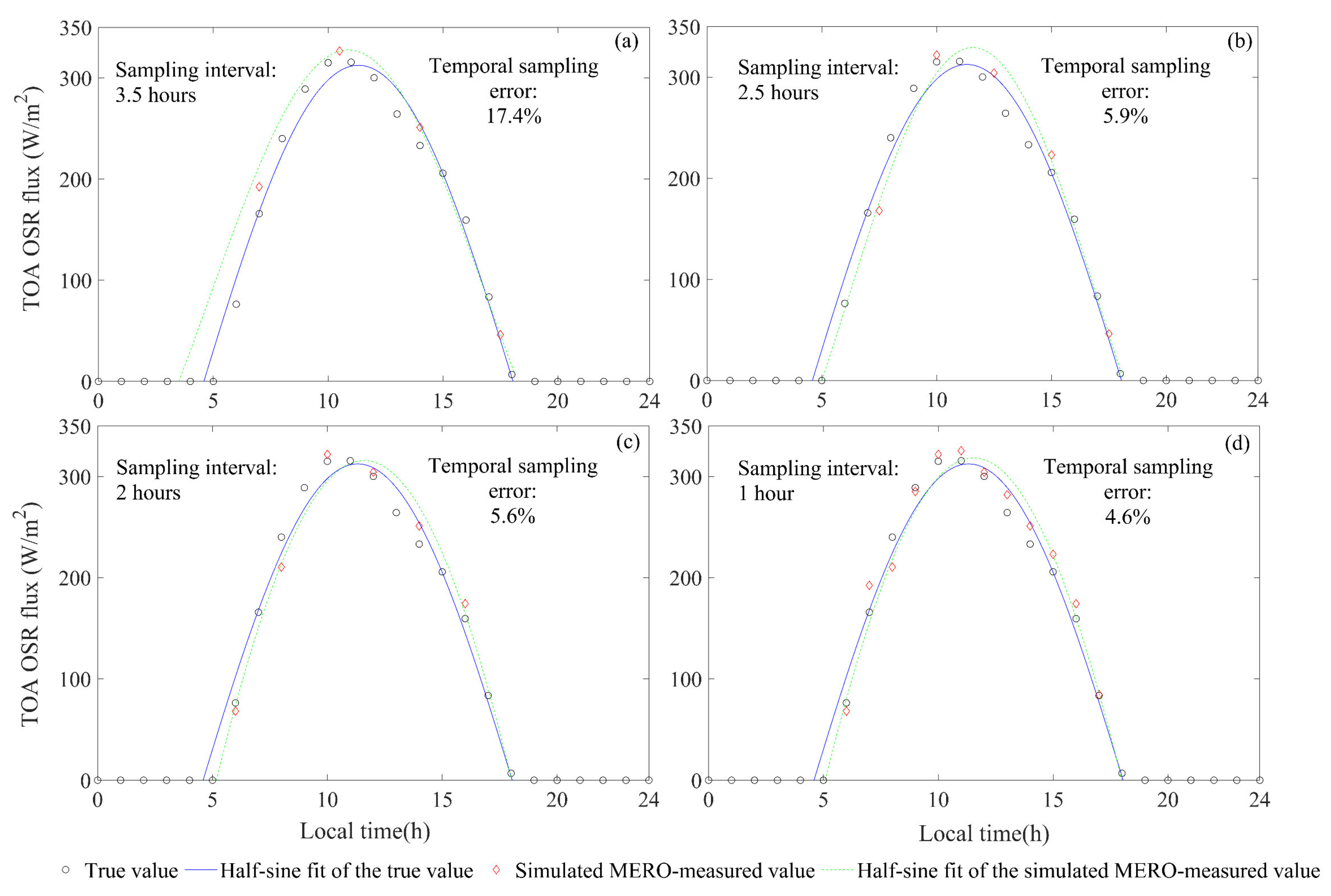
3.2.1. Errors Induced by Sampling Interval

As indicated by previous studies [17,21], the continuous diurnal TOA OSR flux could be derived by the half-sine fitting of daytime samples, due to the nearly half-sine shape of the diurnal cycle solar insolation, whereas the continuous diurnal TOA OLR flux could be derived by the half-sine fit of the daytime samples and linear interpolation of the night-time samples. Therefore, the measurement error is substantially affected by the amounts of samples in the general case; more samples will result in better constraints for the interpolation of the measurement value (Figure 6), making the fitted measurement curve closer to the true value curve. For example, the sampling interval of 3.5 h make just 4 daytime OSR measurement samples (Figure 6a); the top and left slope of the half-sine measurement fit curve are poorly constrained, hence resulting in a relatively high OSR temporal sampling error (17.4%), whereas the sampling interval of 1 h could produce 12 daytime OSR measurement samples (Figure 6d), which covers almost the bottom, the left and right slope, and the peak of the half-sine measurement fit curve, therefore resulting in a smaller error (4.6%).

Although the increase of the temporal samples leads to a better accuracy, such promotion would vanish when the sampling interval reach a threshold (Figure 7). For the OSR flux, this threshold is 1.5 h, sampling intervals of 1.5 h would make 16 temporal samples in a diurnal cycle, where nearly 8 to 9 is at daytime to cover the important positions (peak, two bottoms and the left and right slopes) of the half-sine fitting curve, making a good constraint on the fitting curve. Interpolation with sampling intervals bigger than 1.5 h would misfit some of these important positions; therefore, the change of the sampling interval within the range of >1.5 h would result in an evidence variance in the OSR measurement error. On the contrary, interpolation with sampling intervals of less than 1.5 h would just make a slight improvement to the constraint of the fitting curve compared to the 1.5-h-sampling-interval interpolation; hence, variation in the sampling interval within the range of <1.5 h would not make a significant change in the OSR measurement error. It is also indicated that the measurement error of the TOA OSR flux stays around 5% when the sampling interval is less than the threshold (1.5 h). This near constant 5% error results from the systematic error of a single sample, which would produce a certain offset between the measurement fitting curve and the true value interpolating curve no matter what the sampling intervals is. In our sampling interval assessment, the main source of this systematic error is the utilized fixed spatial resolution (40 km), which would result in an around 5% measurement error (Figure 5). For the OLR flux, this sampling measurement error threshold is 2 h, and a less-than-2 h sampling interval would result in a near constant 5% measurement error. Note that the measurement error threshold of TOA OSR flux (1.5 h) is less than that of the TOA OLR flux (2 h). This is because the amplitude of TOA OSR flux curve is much larger than the TOA OLR flux in a diurnal cycle (OSR flux is larger than 300 W/m²; OLR flux is less than 50 W/m²), and the OSR half-sine lateral slope is much steeper than the OLR, hence more sampling points are needed to constrain the OSR fitting curve than the OLR. However, in actual operation of a MERO mission, the systematic error of OSR and OLR fluxes would come from several other sources despite the spatial resolution. For example, quality of the radiative calibration is also an important systematic error source (the radiative calibration corrects the function of true received radiation before the optical system against the final output DN (digital number) values). The degradation of the MERO sensor caused by the high-energy particles on the Moon would substantially alter the function of the actual true received radiation against the DN value; if the calibration frequency could not catch the degrading speed, there will exist large measurement errors in the final data products. Therefore, a good protection system against the high-energy particles and a feasible in-situ calibration method are crucial for a MERO system (the inbuild calibration system would also degrade and, hence, is less reliable).

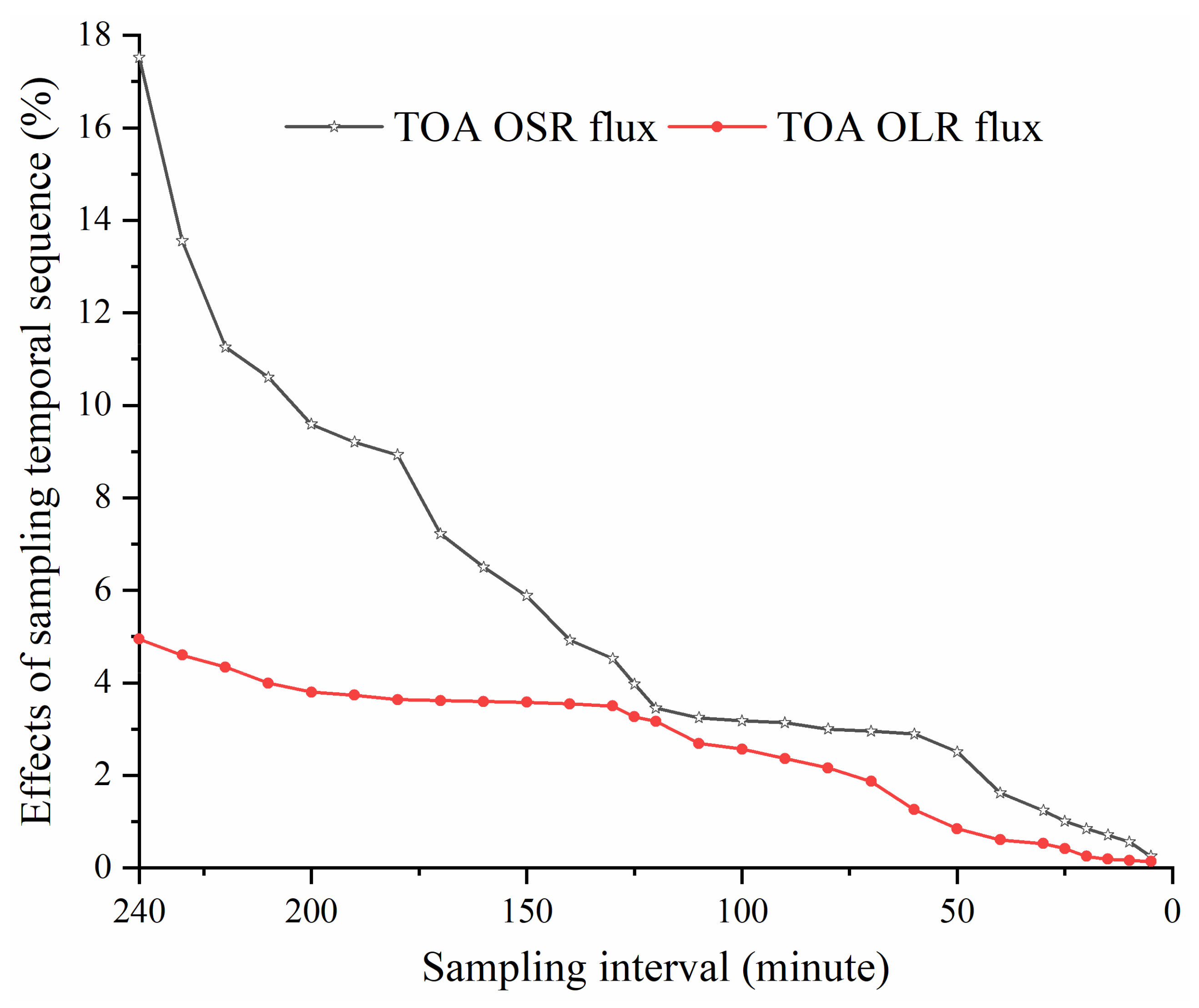
3.2.2. Errors Induced by Sampling Temporal Sequence

As indicated in Figure 6, the shape of the estimated-MERO-measured flux fitting curve is strongly correlated with the distribution of the discretized temporal samples; if the temporal samples cover the vital control positions (the bottoms, the ascent and descent slopes and the peaks), the estimated-MERO-measured flux fitting curve would get close to the true value curve, thus resulting in less error. By contrast, fitting with the uncovering of these important positions would lead to a bigger measurement error. This indicates that a suitable sampling temporal sequence, which would alter the distribution of the discretized temporal samples under a fixed sampling interval, is crucial for a MERO mission. For example, under the fixed sampling interval of 2 h, a sampling temporal sequence with a start at local time of 16 min balanced covers the left and right slope bottoms, the ascend and descend slops and the top of the half-sine fit curve of the OSR measurement, which serves as a strong constraint on the opening extension and shape of the fitting curve (Figure 8a), whereas temporal sequence with a start at local time of 104 min (Figure 8b) tends to the left slope, making the opening extension and the shape of the fitting curve less constrained; therefore, sampling temporal sequence with a start time of 16 min would result in a smaller measurement error (3.9%) than the sampling temporal sequence with a start time of 104 min (6.9%).

A detailed description of the effect of sampling temporal sequence on the measurement error is illustrated in Figure 9; such effects under different sampling intervals have different extent (maximum error minus minimum error). For example, the effect ranges of the OSR and OLR fluxes under 2 h sampling interval are 3.45% and 3.17%, respectively, which are higher than those under a 1.5 h sampling interval (3.14% for OSR and 2.35% for OLR). This is because smaller sampling intervals have more temporal samples, which cover larger parts of the half-sine fit curve; a change of the temporal sampling sequence would have less effect on the shape of the fitting curve, leading to less variation in the measurement error. To fully assess the sampling temporal sequence effect on the measurement error under different sampling intervals, we define the sampling temporal sequence influence at a certain sampling interval as the effect range mentioned above. For example, the effect ranges of sampling temporal sequence on measurement error under a sampling interval of 2 h for TOA OSR and OLR fluxes are 3.45% and 3.17%, respectively (Figure 9a). The full assessment of the effect of sampling temporal sequence on measurement error under different sampling intervals is illustrated in Figure 10. It is found that the TOA OSR flux has a wide range of influence from the sampling temporal sequence (0.6–17.5%), while that of OLR is relatively smaller (0.2–4.9%). This is because the amplitude of the TOA OSR flux half-sine curve is much larger than the TOA OLR flux (OSR flux is larger than 300 W/m²; OLR flux is less than 50 W/m²); the same change of sampling temporal sequence would make a larger offset to the OSR curve than the OLR curve, which would result in a more distinct OSR measurement error change than the OLR observations.

4. Discussion

The Earth energy budget is determined by the radiant energy flow of the Earth. In general, the incoming solar radiation (about 341 W/m²) is partially reflected by the clouds and atmosphere (about 79 W/m²) and by the surface (about 23 W/m²⁾); the remainder is absorbed by the atmosphere (about 78 W/m²) and the surface (161 W/m²). When the surface is heated, it will emit approximately 396 W/m² longwave radiation upward, of which just 40 W/m² could pass through the atmosphere to the outer space and the rest is absorbed by the atmosphere (356 W/m²). When the atmosphere is heated, it would emit about 199 W/m² upward to the outer space and about 333 W/m² downward back to the surface [22]. In this case, the energy budget at Earth TOA is balanced; the incoming solar energy (341 W/m²) is equal to the outgoing radiant energy (the OSR: about 102 W/m² and the OLR: nearly 239 W/m²). This balanced Earth radiation budget may be the actual case in a relatively long period (such as the magnitude of hundreds of years or larger). However, several studies reported that the Earth radiation energy is imbalanced in recent decades; the outgoing radiation is less than the incoming solar radiation by approximately 0.71 W/m² [23], possibly due to the anthropogenic emissions of greenhouse gases. Such an Earth radiation imbalance (ERI) is vital to the synoptic and climate change. Nevertheless, current space-based ERB missions quantify the absolute value of the ERI with large uncertainty, which cannot satisfy the required “climate accuracy” due to the limited temporal sampling coverage and the non-simultaneous sampling of the spatial-temporal variability. As a next-generation Earth radiation budget mission, a MERO could overcome these limitations through the long-term continuous measurement of OSR and OLR in the diurnal cycle and simultaneous half-globe OSR and OLR observations.

Generally, a detector would output an averaging value to blur the actual variance of the OSR and OLR fluxes within the pixel GFOV (ground field of view, which is the actual Earth TOA area that a pixel covers), thus resulting in certain errors. This error would become larger when the size of the pixel GFOV increased. For a MERO system, the border detector unit therefore possesses larger measurement error than the middle one, due to the larger GFOV of the border pixel caused by the Earth surface curvature. Accordingly, controlling the measurement error of border pixels is crucial to reduce the spatial-resolution-induced error of the whole system.

As indicated above, the sampling-scheme-induced error is comprised of two parts: the sampling-interval-induced error (Figure 7) and the sampling-sequence-induced error (Figure 10). For a MERO system with a 40 km spatial resolution, the sampling-interval-induced measurement error of the TOA OSR flux stays around 5% when the sampling interval is less than 90 min; such a threshold is 120 min for the TOA OLR flux (Figure 7). This indicates that reducing measurement error by reducing the sampling interval has a limitation under certain spatial resolutions. Since more temporal samples need better capability for data storage and transmission (higher manufacturing cost), setting the sampling interval as the measurement error threshold indicated above could guarantee the nearly smallest measurement error with the least manufacturing cost (for example, 90 min is the best sampling interval for MERO with a spatial resolution of 40 km). After the best sampling interval is set (90 min), it is necessary to ascertain the temporal sampling sequence that result in the least measurement error. It is indicated that the sampling sequence starting time of 63 min would result in a least measurement error of the TOA OSR flux, and a starting time of 64 min would result in the least measurement error of the TOA OLR flux (Figure 9b). Therefore, a sampling temporal sequence with a starting time of 64 min with a sampling interval of 90 min ought to be the optimal sampling scheme for a MERO with a 40 km spatial resolution.

Our results indicate that the temporal sampling error do not change when the sampling interval is less than or near 1 h for both the TOA OSR and OLR fluxes; however, this may not be the fact. We chose the 1 hourly CERES OSR/OLR data and interpolated it to 1 min temporal resolution, which is then be regarded as the “true value” in our study. Afterward, this true value is used to simulate the MERO-measured OSR/OLR flux. We choose the CERES measurements as “true data” since CERES is currently one of the most reliable ERB systems around the world and because the CERES data is consistent with the CERES ADMs we used in our study, which is the core function to generate the TOA OSR/OLR anisotropic factors. However, such a 1 min interpolated true value is smoothed between two 1-h samples (Figure 2), which neglects the actual less-than-1-h temporal variability of the TOA OSR and OLR fluxes. As such, the temporal sampling error would have little change when the sampling interval is less than 1 h, which can be interpreted as follows: 1. for the true data, the 1 min interpolation is based on the 1 hourly CERES data, and the information of less-than-1-h OSR/OLR variation is lost (see Figure 2); therefore, the shape of the true OSR/OLR diurnal curve is actually determined by the original 12/24 key temporal samples (the OSR curve only exist at daytime; OSR at nighttime stays at 0); the newly interpolated 1 min temporal points do not affect the curve shape (see Figure 2); 2. the simulated MERO measured OSR/OLR flux variation is calculated based on the true data curve; therefore, the less-1-h OSR/OLR variability of the simulated MERO-measured curve is also lost. When the sampling interval is less than or near 1 h, the newly calculated value would have less effect on the simulated MERO-measured OSR/OLR flux variation curve, leading to a relatively unchanged temporal sampling error. We think that a more realistic TOA OSR and OLR flux data with better temporal resolution (such as 10 min) could help to figure out the actual temporal sampling error when the sampling interval is less than 1 h. The CMIP 6 (Coupled Model Intercomparison Project Phase 6) generated data along with the GERB measurements may be a feasible way, which we would try in our future work.

In the actual design of a MERO system, the spatial resolution could be ascertained by the balance between the spatial-resolution-induced error and the manufacturing cost using the spatial resolution assessment results derived in our study. Then the optimal sampling scheme could be determined through the method we proposed above for a MERO with a spatial resolution of 40 km.

In this study, we evaluated the temporal sampling scheme induced error during March 2019, since both the Arctic and Antarctic has TOA OSR during this month. However, since the OSR and OLR for the summer and winter months have very different radiative flux distributions than those of the transitional months (spring and autumn), the full assessment of this sampling-scheme-induced error over four seasonal months could result in better results. We would conduct this study in the further work.

We assessed the spatial resolution at an extensive range from 1000 km to 20 km to facilitate the scientific design of a MERO with consideration of the state of art and future advances in technology. For example, considering an assumed case that the MERO can only have a spatial resolution of 50 km and a temporal resolution of 1 h under the limitation of the state of the art and mission fund budget, this paper can help to give the corresponding measurement error caused by spatial-temporal resolution, which is part of the inherent error of a MERO system. Instead, if our assessment range is too small (for example, 1000 km–100 km), the spatial-temporal-resolution-induced error of the MERO system in the above case cannot be derived. This would make our study less valuable. Therefore, the extensive range of spatial resolution (1000 km to 20 km) and temporal resolution (240 min to 1 min) of this study is useful with consideration of the state of the art and future improvement of the technology, though the maximum of the spatial resolution and temporal resolution cannot be reached under the state of the art.

The MERO instrument has a focal plane array (FPA) with a multi-detector unit, and each unit views a part of the Earth TOA (represented by a pixel), respectively (Figure 3); therefore, the generated data is the multi-pixel image of TOA OSR and OLR fluxes. In the actual MERO operation stage, the received irradiance of one detector will be converted to the Earth TOA flux of the corresponding pixel using an anisotropic factor; the anisotropic factor of one pixel is the ratio of the received radiance by the corresponding detector to the Earth TOA flux (Equation (2)). Therefore, the pixel-scale anisotropic factor is vital for the data-producing of the MERO system. To calculated the pixel-scale anisotropic factor, we used the numerical discretizing method: the pixel is discretized into sub grid points, and one grid point represents one TOA area of 0.1° latitude × 0.1° longitude (discretization of pixel 8’ in Figure 3), then the anisotropic factors of these sub grids are area-weighting summed to derive the anisotropic factor of the whole pixel (Equation (3)). The OSR and OLR anisotropic factors of one sub grid are derived by the CERES angular distribution models (ADMs) [19,20]. The ADMs generate the TOA OSR/OLR anisotropic factor based on the scene type by considering their dependence on the viewing geometry, the beneath surface type and the related cloud and meteorological parameters. In the ADMs, every OSR/OLR scene type corresponds to one TOA OSR/OLR anisotropic factor, respectively; when the scene type is confirmed, the anisotropic factor can be derived. ADMs describe the scene type by a discrete bin method: related parameters (surface type, related cloud and meteorological parameters, viewing geometry angles, see Table 1 and Table 2) are discretized into several bins, a possible combination of bins of every of these parameters is set as one scene type. In the actual operation of a MERO mission, the meteorological parameter and surface-type data mentioned above should be firstly derived to generate the real-time OSR/OLR anisotropic factors for every pixel. The surface type can be determined by the IGBP or NOAA JPSS-VIIRS-AST global surface data or other global surface-type products. The meteorological parameters could be derived through mounting a meteorological observation payload (like MODIS (moderate-resolution imaging spectroradiometer)) on the MERO or by utilizing the global meteorological database.

The real-time instantaneous regionally half-globe Earth TOA OSR and OLR images are the basic category of the MERO dataset, which are generated as follows. At one time point, the focal plane detector array (FPA) (ensemble of amounts of individual detector units) of the MERO system would “photograph” the full Earth disk instantaneously; every detector unit just simultaneously “photographs” the OSR/OLR radiation of part of the Earth TOA (represented by an image pixel) respectively (see Figure 3) [24]. The left bottom hollow green rectangle in Figure 1 shows the example of one image pixel; the upper right solid green rectangle is the corresponding detector unit. In the FPA, one detector unit is an individual system; it converts the received radiation of the pixel to the electrical signal and process it to a digital number, then this digital number is converted to the incident flux by radiometric calibration function, and such an incident flux would afterward be converted to the incident radiance using the MERO observing geometry. This incident radiance would be then converted to the flux of the corresponding image pixel using the anisotropic factor (Equation (2)). At last, when all the OSR/OLR fluxes of the image pixels are derived, the instantaneously regional half-globe TOA OSR/OLR fluxes image at the time point can be derived. After geometrically correcting and projecting (or resampling) the image to the regular Earth discretized grids, the MERO instantaneous regionally half-globe OSR/OLR flux map at that time point could be derived.

5. Conclusions

A MERO could bring several improvements to current ERB observations: (1) long-term continuous observation in a diurnal cycle for a region on Earth (12-h continuous observation per day) enables a MERO to capture the small-temporal-scale variations of the TOA OLR and OSR, benefiting the production of a more accurate measurement of OLR and OSR diurnal variations; (2) a MERO could simultaneously measure the half-globe TOA OSR and OLR fluxes at an acceptable spatial resolution; this could help to shed light on the regional and global radiation imbalance without the bias caused by non-simultaneous sampling of the spatial and temporal variability of TOA OSR and OLR; (3) all locations on the Moon share a highly similar viewing geometry towards Earth, facilitating the merging of data from MERO missions of different periods to produce long-term OSR and OLR data with good consistency; (4) a MERO could provide a longer-term observation within a diurnal cycle for polar regions compared to current LEO and GEO ERB missions.

In this paper, we quantify the effects of the spatial resolution and sampling scheme on the measurement error for a Moon-Based Earth Radiation Observatory (MERO). It is found that the spatial sampling error in the unit of percentage reduces linearly as the spatial resolution varies from 1000 km to 100 km; the rate is 2.5%/100 km for the TOA OSR flux, which is higher than that (1%/100 km) for TOA OLR flux. Moreover, this rate becomes larger when the spatial resolution is less than 40 km. It is also shown that sampling temporal sequence with a starting time of 64 min and with a sampling interval of 90 min is the optimal sampling scheme that results in the least temporal sampling error for a MERO system with a 40 km spatial resolution; however, due to the “real” TOA OSR and OLR fluxes are based on the 1-h CERES data in this study, which neglect the actual data variability that is less than 1 h, this conclusion still can be improved by utilizing a more realistic TOA fluxes dataset in higher temporal resolution. The proposed method and the derived results in this study could help to determine the optimal spatial resolution and sampling scheme (sampling interval and the temporal sampling sequence) of a MERO system under specific manufacturing budget and measurement error limits.

References

1. Brown, P.T.; Caldeira, K. Greater future global warming inferred from Earth’s recent energy budget. Nature 2017, 552, 45–50. [Google Scholar] [CrossRef]
2. Barkstrom, B.R.; Smith, G.L. The Earth Radiation Budget Experiment: Science and implementation. Rev. Geophys. 1986, 24, 379–390. [Google Scholar] [CrossRef]
3. Wielicki, B.A.; Barkstrom, B.R.; Harrison, E.F.; Iii, R.B.L.; Smith, G.L.; Cooper, J.E. Clouds and the Earth’s Radiant Energy System (CERES): An Earth Observing System Experiment. Bull. Am. Meteorol. Soc. 1996, 77, 853–868. [Google Scholar] [CrossRef] [Green Version]
4. Smith, G.L.; Priestley, K.J.; Loeb, N.G. Clouds and Earth Radiant Energy System: From Design to Data. IEEE Trans. Geosci. Remote Sens. 2014, 52, 1729–1738. [Google Scholar] [CrossRef]
5. Harries, J.E.; Russell, J.; Hanafin, J.; Brindley, H.; Futyan, J.; Rufus, J.; Kellock, S.; Matthews, G.; Wrigley, R.; Last, A. The geostationary earth radiation budget project. Bull. Am. Meteorol. Soc. 2005, 86, 945–960. [Google Scholar] [CrossRef] [Green Version]
6. Burt, J.; Smith, B. Deep Space Climate Observatory: The DSCOVR mission. In Proceedings of the 2012 IEEE Aerospace Conference, Big Sky, MT, USA, 3–10 March 2012; pp. 1–13. [Google Scholar]
7. Smith, G.L.; Wong, T. Time-Sampling Errors of Earth Radiation From Satellites: Theory for Monthly Mean Albedo. IEEE Trans. Geosci. Remote Sens. 2016, 54, 3107–3115. [Google Scholar] [CrossRef]
8. Smith, G.L.; Wong, T.; Bush, K.A. Time-Sampling Errors of Earth Radiation From Satellites: Theory for Outgoing Longwave Radiation. IEEE Trans. Geosci. Remote Sens. 2015, 53, 1656–1665. [Google Scholar] [CrossRef]
9. Dewitte, S.; Gonzalez, L.; Clerbaux, N.; Ipe, A.; Bertrand, C.; De Paepe, B. The Geostationary Earth Radiation Budget Edition 1 data processing algorithms. Adv. Space Res. 2008, 41, 1906–1913. [Google Scholar] [CrossRef]
10. Duan, W.; Huang, S.; Nie, C. Conceptual design of a Moon-Based Earth Radiation Observatory. Int. J. Remote Sens. 2018, 39, 5834–5849. [Google Scholar] [CrossRef]
11. Wielicki, B.A.; Young, D.F.; Mlynczak, M.G.; Thome, K.J.; Leroy, S.; Corliss, J.; Anderson, J.G.; Ao, C.O.; Bantges, R.; Best, F.; et al. Achieving Climate Change Absolute Accuracy in Orbit. Bull. Am. Meteorol. Soc. 2013, 94, 1519–1539. [Google Scholar] [CrossRef] [Green Version]
12. Swartz, W.H.; Lorentz, S.R.; Papadakis, S.J.; Huang, P.M.; Smith, A.W.; Deglau, D.M.; Yu, Y.; Reilly, S.M.; Reilly, N.M.; Anderson, D.E. RAVAN: CubeSat Demonstration for Multi-Point Earth Radiation Budget Measurements. Remote Sens. 2019, 11, 796. [Google Scholar] [CrossRef] [PubMed] [Green Version]
13. Meftah, M.; Damé, L.; Keckhut, P.; Bekki, S.; Sarkissian, A.; Hauchecorne, A.; Bertran, E.; Carta, J.-P.; Rogers, D.; Abbaki, S.; et al. UVSQ-SAT, a Pathfinder CubeSat Mission for Observing Essential Climate Variables. Remote Sens. 2020, 12, 92. [Google Scholar] [CrossRef] [Green Version]
14. Wong, T.; Smith, G.L.; Kato, S.; Loeb, N.G.; Kopp, G.; Shrestha, A.K. On the Lessons Learned From the Operations of the ERBE Nonscanner Instrument in Space and the Production of the Nonscanner TOA Radiation Budget Data Set. IEEE Trans. Geosci. Remote Sens. 2018, 56, 5936–5947. [Google Scholar] [CrossRef] [PubMed]
15. Loeb, N.G. Ceres SYN ED4A Data Quality, 4th ed.; CERES Science Team, Ed.; NASA Atmospheric Science Data Center (ASDC): Hampton, VA, USA, 2017.
16. Nascimento, G.d.S.; Ruhoff, A.; Cavalcanti, J.R.; Marques, D.d.M.; Roberti, D.R.; Rocha, H.R.d.; Munar, A.M.; Fragoso, C.R.; Oliveira, M.B.L.d. Assessing CERES Surface Radiation Components for Tropical and Subtropical Biomes. IEEE J. Sel. Top. Appl. Earth Obs. Remote Sens. 2019, 12, 3826–3840. [Google Scholar] [CrossRef]
17. Doelling, D.R.; Loeb, N.G.; Keyes, D.F.; Nordeen, M.L.; Morstad, D.; Nguyen, C.; Wielicki, B.A.; Young, D.F.; Sun, M. Geostationary enhanced temporal interpolation for CERES flux products. J. Atmos. Ocean. Technol. 2013, 30, 1072–1090. [Google Scholar] [CrossRef]
18. Duan, W.; Huang, S.; Nie, C. Entrance Pupil Irradiance Estimating Model for a Moon-Based Earth Radiation Observatory Instrument. Remote Sens. 2019, 11, 583. [Google Scholar] [CrossRef] [Green Version]
19. Su, W.; Corbett, J.; Eitzen, Z.; Liang, L. Next-generation angular distribution models for top-of-atmosphere radiative flux calculation from CERES instruments: Methodology. Atmos. Meas. Tech. 2015, 7, 611–632. [Google Scholar] [CrossRef] [Green Version]
20. Loeb, N.G.; Kato, S.; Loukachine, K.; Manalo-Smith, N. Angular Distribution Models for Top-of-Atmosphere Radiative Flux Estimation from the Clouds and the Earth’s Radiant Energy System Instrument on the Terra Satellite. Part I: Methodology. J. Atmos. Ocean. Technol. 2005, 22, 338–351. [Google Scholar] [CrossRef]
21. Wielicki, B.A.; Green, R.; Tolson, C.; Fan, A. Clouds and the Earth’s Radiant Energy System (CERES) Algorithm Theoretical Basis Document; Atmospheric Sciences Division, NASA Langley Research Center: Hampton, VA, USA, 1995.
22. Trenberth, K.E.; Fasullo, J.T.; Kiehl, J. Earth’s global energy budget. Bull. Am. Meteorol. Soc. 2009, 90, 311–323. [Google Scholar] [CrossRef]
23. Loeb, N.G.; Doelling, D.R.; Wang, H.; Su, W.; Nguyen, C.; Corbett, J.G.; Liang, L.; Mitrescu, C.; Rose, F.G.; Kato, S. Clouds and the Earth’s Radiant Energy System (CERES) Energy Balanced and Filled (EBAF) Top-of-Atmosphere (TOA) Edition-4.0 Data Product. J. Clim. 2018, 31, 895–918. [Google Scholar] [CrossRef]
24. Rogalski, A. Progress in focal plane array technologies. Prog. Quantum Electron. 2012, 36, 342–473. [Google Scholar] [CrossRef]
Figure 1. The typical observing scenario of a MERO system and the pathway of the radiation from the pixel on the Earth top of atmosphere (TOA) (hollow green rectangle) to the detector unit (solid green rectangle) of the focal plane array of the MERO.
Remotesensing 13 04432 g001
Figure 2. The selected true hourly TOA Earth TOA (a) OSR flux and (b) OLR flux data and the temporal interpolations to derive the 1-min true OSR and OLR fluxes of a location on Earth (20° E, 30° S). The true hourly data comes from the CERES SYN dataset of March 2019.
Remotesensing 13 04432 g002
Figure 3. The correlation of a detector array and a pixel array of a MERO system. A pixel is discretized into sub grid points (such as pixel 8’); each sub grid point represents an Earth TOA area of 0.1° latitude × 0.1° longitude.
Remotesensing 13 04432 g003
Figure 4. Geometries of the viewing zenith angle (vi), the relative azimuth angle (ri), the solar zenith angle (si), and Earth’s viewing angle (ωi) of a MERO sensor towards a sub grid point i within a pixel on the Earth TOA (top of the atmosphere).
Remotesensing 13 04432 g004
Figure 5. Pixel-averaged spatial sampling error as a function of spatial resolution of a MERO system (range of spatial resolution is 1000 km–20 km, step at the range of 1000 km–100 km is 100 km, step at the range of 100 km–10 km is 10 km).
Remotesensing 13 04432 g005
Figure 6. Comparisons of the true and the simulated MERO-measured TOA OSR fluxes of an Earth’s location (0° E, 40° S) in March 2019 under sampling intervals of (a) 3.5 h, (b) 2.5 h, (c) 2 h and (d) 1 h, respectively.
Remotesensing 13 04432 g006
Figure 7. Temporal sampling error induced by sampling intervals under a constant sampling temporal sequence (start time of 0 min); range of the sampling interval is 240 min–1 min; step is 10 min at the range of 240 min–20 min’ step is 1 min at the range of 20 min–1 min.
Remotesensing 13 04432 g007
Figure 8. Comparisons of the true and simulated MERO-measured TOA OSR fluxes under a fixed sampling interval of 2 h (a) with the sampling temporal sequence in the start time of 16 min and (b) with the sampling temporal sequence in the start time of 104 min.
Remotesensing 13 04432 g008
Figure 9. Effect of sampling temporal sequence on the measurement error under (a) a sampling interval of 2 h and (b) a sampling interval of 1.5 h; the sampling temporal sequence start time step is 1 min.
Remotesensing 13 04432 g009
Figure 10. The effect of sampling temporal sequence on the measurement error under various sampling intervals; the range of the sampling interval is 240 min–1 min; step is 10 min at the range of 240 min–20 min; step is 1 min at the range of 20 min–1 min.
Remotesensing 13 04432 g010