Assessment of Urban Ecological Quality and Spatial Heterogeneity Based on Remote Sensing: A Case Study of the Rapid Urbanization of Wuhan City

Abstract

Rapid urbanization significantly affects the productivity of the terrestrial ecosystem and the foundation of regional ecosystem services, thereby detrimentally influencing the ecological environment and urban ecological security. The United Nations’ Sustainable Development Goals (SDGs) also require accurate and timely assessments of where people live in order to develop, implement and monitor sustainable development policies. Sustainable development also emphasizes the process of protecting the ecological environment for future generations while maintaining the current needs of mankind. We propose a comprehensive evaluation method for urban ecological quality (UEQ) using Landsat TM/ETM+/OLI/TIRS images to extract remote sensing information representing four ecological elements, namely humidity, greenness, heat and dryness. An improved comprehensive remote sensing ecological index (IRSEI) evaluation model is constructed by combining the entropy weight method and principal component analysis. This modeling is applied to the city of Wuhan, China, from 1995 to 2020. Spatial autocorrelation analysis was conducted on the geographic clusters of the IRSEI. The results show that (1) from 1995 to 2015, the mean IRSEI of Wuhan city decreased from 0.60 to 0.47, indicating that environmental deterioration overwhelmed improvements; (2) the global Moran’s I for IRSEI ranged from 0.535 to 0.592 from 1995 to 2020, indicating significant heterogeneity in its spatial distribution, highlighting that high and low clusters gradually developed at the edge of the city and at the city center, respectively; (3) the high clusters are mainly distributed in the Huangpi and Jiangxia districts, and the low clusters at the city center, which exhibits a dense population and intense human activity. This paper uses remote sensing index methods to evaluate UEQ as a scientific theoretical basis for the improvement of UEQ, the control of UEQ and the formulation of urban sustainable development strategies in the future. Our results show that the UEQ method is a low-cost, feasible and simple technique that can be used for territorial spatial control and spatiotemporal urban sustainable development.

1. Introduction

Urban ecological quality (UEQ) evaluation is an important field of urban ecology research and the basis of urban planning and ecological management. With the continuous expansion of urbanization, China’s cities have achieved medium-high quality development. However, social problems, such as resource exhaustion, an imbalance of economic structure and environmental pollution, do appear frequently. It is urgent to improve the capacity to implement urban sustainable development. In 2015, United Nations (UN) member states unanimously committed to achieving the Sustainable Development Goals (SDGs) by 2030 [1]. Although the urbanization process has improved people’s living standards, promoted the sustainable development of productive forces and provided economic benefits, it has also broken the balance between human society and the natural environment, and has brought great challenges to UEQ [2,3]. According to the 2018 Revision of World Urbanization Prospects [4,5], the urban population will account for 68% of the global population by 2050, which is an increase of 13% from 2018, and China’s urban population will increase by 255 million people. Cities cover less than 2% of the Earth’s surface, but consume 78% of the energy generated and produce 60% of greenhouse gas emissions [5]. Additionally, urban land consumption outpaces population growth by approximately 50% [6].

Such changes affect human survival and the sustainable development of the social economy [7,8,9,10]. Using UEQ measures to determine the status of the ecological environment could promote the sustainable development of regional economies [8,11,12,13,14]. Therefore, the quantitative description and assessment of the spatiotemporal dynamics of urban ecological environments are emerging as leading research topics [11,15].

Numerous studies have been conducted on such an assessment from different perspectives, and several evaluation methods have been suggested. The pressure–state–response model and fuzzy evaluation methods are commonly used in ecological quality assessment. In recent years, geographic information system (GIS) and remote sensing (RS) technologies have provided efficient monitoring and analysis methods for ecological quality research and sustainable development. Progress in satellite-based Earth observation systems facilitates assessing the state of an ecosystem from local to global scales. The scale and scope of this research are expanding constantly. Index systems have been constructed using GIS to conduct strategic environmental assessment for regional and land-use planning [16,17]. In China, research on the ecological environment is based on the Technical Specifications for Ecological Environmental Assessment, promulgated by the National Environmental Protection Agency in 2006 [18]. According to these specifications, the ecological environment index (EI) should encompass biological richness, air pollution, water network density, vegetation cover, land degradation and related factors. The EI is the main tool used to evaluate the quality of the ecological environment [19]. However, as climatic and geological conditions differ across regions, the weight of each index must be adjusted accordingly. Currently, researchers mostly use manual processing, as weight allocation is not strictly required and evaluation criteria vary, making it extremely difficult to accurately compare urban ecological conditions. Therefore, a scientific and logical ecological quality assessment method is required.

The acceleration of urbanization has led to a series of ecological and environmental effects, such as reduced surface water transpiration and water quality. It is generally difficult to monitor these natural processes with on-site instruments. However, remote sensing technologies can provide quantitative physical data with high spatial and temporal resolutions to facilitate the quantitative monitoring and analysis of environmental effects. Among all of the environmental effects of urbanization, the thermal environment has received more attention. The urban thermal environment is an important representative indicator of the urban environment. It is influenced by the physical properties of the urban surface and human social and economic activities, and is a comprehensive summary and embodiment of urban ecosystems. Vegetation is another important component of urban ecosystems. Urban vegetation can selectively absorb and reflect solar radiation energy, adjust the latent and sensible heat exchange, regulate urban air, reduce pollution and other processes that affect the city’s natural environment and is another highly comprehensive index of urban ecological evaluation. The spatial distribution and richness of vegetation in cities have always been considered to have important effects on the evolution of the urban ecological environment.

The remote sensing ecological index (RSEI) combines humidity, greenness, heat and dryness indices obtained from RS, and facilitates the monitoring and evaluation of the UEQ. The RSEI, which was first proposed by Hu and Xu [18], could aid in visualizing spatial and temporal analyses and predictions of change in the regional environment, thereby compensating for the deficiencies of the EI. This paper uses existing research from a new perspective to more accurately study urban socio-economic activity intensity and its relationship with the regional ecological environment. Using the RSEI will help in studying the interactions between human activities and natural ecology, and the resulting knowledge of theory, concepts and methods is expected to benefit local governments [20]. In recent years, the RSEI has been applied in ecological quality monitoring in 35 cities of China [19,21,22], Eurasia [23] and America [21,23]. The RSEI and the results of principal component analysis (PCA) have been combined to develop an ecological index [19,24]. However, using the PCA results in insufficient information utilization, as the adaptive nature of PCA algorithms inevitably limits the full use of the available information. For example, the RSEI obtained in two studies using only the first component for normalization ranged from 60% to 90%, which cannot guarantee adequate contribution rates.

Accordingly, the aim of the current study is to improve the RSEI calculation method by proposing an improved-comprehensive remote sensing ecological index (IRSEI) constructed by employing PCA and equal weights (EW). Our study overcomes the shortcomings of previous studies, which only considered the application of PCA in ecological quality assessment, and the resolved knowledge gaps are reflected in the comprehensive consideration of EW and the PCA method to determine the UEQ. The contribution rates of the eigenvalues of PCA and EW are taken as the weights. This method enables the full use of the available data and ensures that the value of the calculated IRSEI is ecologically optimal. In addition, more indicators could be integrated and the IRSEI reduces noise interference and makes optimal use of practical image information. These factors facilitate the reliable and quantitative monitoring of the regional ecological environment.

A comparison and evaluation of the differences in quality in large cities can improve the cognitive ability of the internal mechanism of the reciprocal feed-back relationship between the construction of megacities and regional ecological balance, and can provide a scientific reference for controlling the scale of urban sustainable development and ecological planning and regulation. Wuhan is one of the fastest growing cities in central China, but few studies have been conducted on quantitative UEQ monitoring based on remote sensing data. Therefore, we used a series of parameters obtained from remote sensing imagery to construct the IRSEI for the evaluation of the UEQ of Wuhan city from 1995 to 2020. In addition to the UEQ, we determined the temporal and spatial changes in the city. We present a discussion of the ecological changes caused by economic and social developments and natural conditions. Finally, we provide theoretical guidance and a scientific basis for ecological construction in Wuhan city.

The objectives of this study are to:

(1)

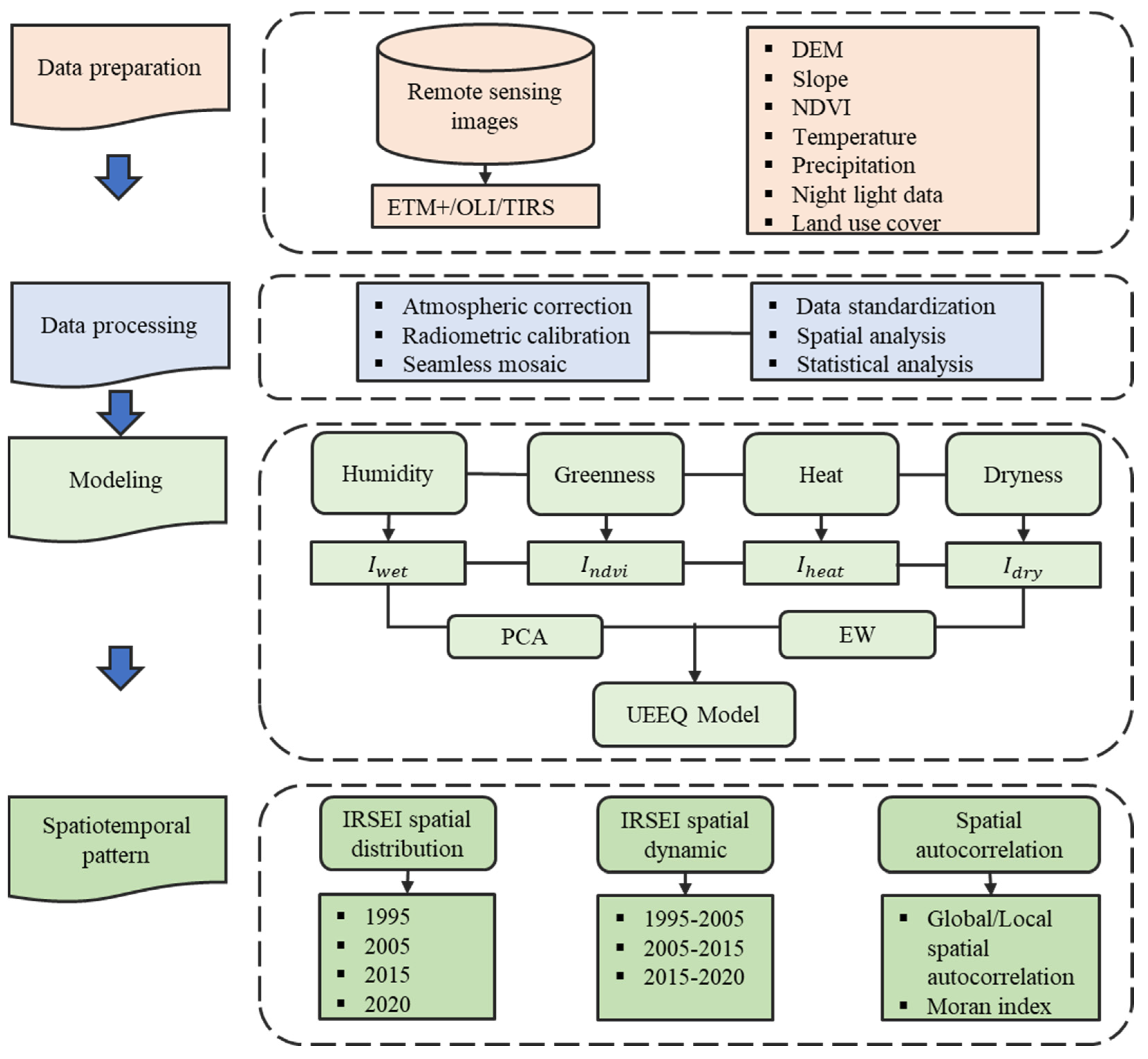
Use GIS and RS technology to construct the IRSEI efficiently by integrating multiple sensors, including the Landsat Thematic Mapper (TM), Operational Land Imager (OLI) and Thermal Infrared Sensor (TIRS);

(2)

Monitor spatial and temporal changes in UEQ in Wuhan from 1995 to 2020;

(3)

Explore the spatial differentiation characteristics of the IRSEI in Wuhan.

2. Materials and Methods

2.1. Study Area and Data Preprocessing

We select the rapidly urbanizing city of Wuhan as study area for ecological monitoring and assessment. Wuhan is the capital city of Hubei Province. Its geographical location is 29°58′–31°22′N and 113°41′–115°05′E (Figure 1). From the perspective of Wuhan’s geographical location and the location of its basin, the development of Wuhan has had great impact on the environment of the whole Yangtze River basin, and even the whole country. Therefore, ecological assessment and policy-based restoration and protection in Wuhan are vital for the ecological restoration of the Yangtze River basin. The city has jurisdiction over six central urban areas and seven distant urban areas. The land area comprises 8494.41 km². The permanent population was 10.91 million in 2018. The Yangtze and Han rivers meet there, forming a geographical pattern referred to as “two rivers and three towns”. Wuhan has a subtropical humid monsoon climate, with abundant rainfall and sufficient heat throughout the year. The average annual temperature is 15.8 to 17.5 °C. The area is rich in ecological resources, with nearly 40% green coverage and more than 10 m² of green space per capita. These ecological resources are crucial for Wuhan to build an ecological civilization city and, therefore, are critical factors in the protection of the ecological environment.

In order to consider the quality of the remote sensing data, such as cloud cover and vegetation condition, we use data from Landsat 5 TM in 1995, Landsat 5 ETM in 2005 and Landsat 8 OLI in 2015 and 2020 as the main remote sensing data. RS data are particularly useful because they can be used for temporal and spatial monitoring [25]. Details on the satellite images used in this study are provided in

Table 1. Data used and their source.

Data Used	Data Acquisition Data	Spatial Resolution	Source
LANDSAT TM	24 October 1995	30 × 30	http://earthexplorer.usgs.gov/ (accessed on 15 May 2021).
LANDSAT ETM	11 September 2005	30 × 30
LANDSAT OLI	28 September 2015	30 × 30
	29 October 2020	30 × 30

. The source dates of the images are relatively close; therefore, differences caused by different seasons and vegetation growth states can be ignored. Owing to topographic differences in images at different times and the influence of illumination and atmospheric factors on surface reflectance, the selected images required preprocessing with radiometric calibration and atmospheric and geometric correction prior to the calculation of the IRSEI. The corrections were performed using the Environment for Visualizing Images (ENVI) software. The Fast Line-of-sight Atmospheric Analysis of Hypercubes (FLAASH) model was used for atmospheric correction to eliminate the radiation error caused by atmospheric absorption and scattering. The accuracy of radiation calibration was more than 95%, and that of atmospheric correction exceeded 85%. Further, the error in geometric correction was controlled to less than 1 pixel. The quadratic polynomial and the nearest neighbor methods were used to correct the geometry of the images and the preprocessed images of the study area were clipped using the vector data of the administrative districts of Wuhan. Other data sources included the administrative zoning map of Wuhan, digital elevation model data of Wuhan from the geospatial data cloud (http://www.gscloud.cn/sources/accessdata/310?pid=302 (accessed on 15 May 2021)) and the cloud platform of geographical national condition monitoring of China (http://www.dsac.cn/DataProduct/Search?&cateID=2010&areaID=18 (accessed on 15 May 2021)). Nighttime light data were obtained from the national geophysical data center (https://www.ngdc.noaa.gov/eog/dmsp/downloadV4com-posites.html (accessed on 15 May 2021)).

2.2. Methodology

2.2.1. Modeling Framework

We combine principal component analysis (PCA) and the entropy value method to design synthetic indicators that facilitate quick and quantitative assessment of UEQ, based on humidity, greenness, dryness and the heat index. Using this method enables prioritizing the natural factors of the ecological evaluation system. The overall framework of IRSEI modeling, as shown in Figure 2, includes four main steps. First, we obtain Landsat Enhanced Thematic Mapper Plus (ETM+)/OLI/TIRS images and perform preprocessing, including atmospheric correction, radiometric calibration and image mosaic (see Section 2.1). Second, we derive four remote sensing indicators: humidity, greenness, dryness and heat. Third, we calculate the PCA components, obtain PC1 and use the entropy method to calculate the results that are used for the construction of the IRSEI. Finally, the characteristics of the spatial and temporal changes in the ecological quality of Wuhan over the past 25 years are determined, and the spatial heterogeneity of the city is analyzed.

2.2.2. Calculation of Component Indices

• Humidity index ($I_{wet}$)

The Kauth–Thomas transform (also called the tasseled hat transform) is a linear transformation method based on multispectral imaging [26,27]. This method is widely used in ecological monitoring for data compression and removal of redundancy. The moisture component obtained by this transform reflects moisture information in the soil and vegetation. A low humidity value indicates severe land degradation, low vegetation cover and a poor ecological environment. A high humidity value indicates sufficient soil moisture, rich surface vegetation cover and a good ecological environment.

In this study, $I_{wet}$ was chosen as the humidity index [28], which is expressed as land surface moisture and is generated from Landsat TM, ETM+ and OLI image reflectance using Equations (1)–(3) [10,23,29]:

$$I_{wet\mathrm{TM}} = 0.0315\rho 1+0.2021\rho 2+0.3102\rho 3+0.1594\rho 4-0.6806\rho 5-0.6109\rho 7$$

(1)

$$I_{wet\mathrm{ETM}+} = 0.2626\rho 1+0.2141\rho 2+0.0926\rho 3+0.0656\rho 4-0.7629\rho 5-0.5388\rho 7$$

(2)

$$I_{wet\mathrm{OLI}} = 0.1511\rho 1+0.1973\rho 2+0.3283\rho 3+0.3407\rho 4-0.7117\rho 5-0.4559\rho 7$$

(3)

where $\rho 1$, $\rho 2$, $\rho 3$, $\rho 4$, $\rho 5$ and $\rho 7$ represent reflectance in bands 1, 2, 3, 4, 5 and 7 of Landsat TM/ETM+ images and reflectance in bands 2, 3, 4, 5, 6 and 7 of Landsat OLI data, respectively.

• Greenness index ($I_{ndvi}$)

The normalized difference vegetation index (NDVI) is often used to monitor vegetation growth [30] and directly reflects the quality of the regional ecological environment. This index is used in the classification of regional land cover, environmental change and vegetation. The NDVI greenness index is computed as follows [31]:

$$I_{ndvi} = \left(\rho 4-\rho 3\right)/\left(\rho 4+\rho 3\right)$$

(4)

where $\rho 4$ represents the reflectance of the near-infrared band and $\rho 3$ represents the reflectance of the red band.

• Heat index ($I_{heat}$)

Land surface temperature (LST) refers to heat, which is related closely to vegetation growth, crop yield, surface water circulation, urbanization, other natural phenomena and processes and human activities [32]. LST can be used as a heat index to reflect the surface ecological environment. Several algorithms use thermal infrared technology to retrieve LST, including the atmospheric correction, single-window and single-channel algorithms. Comparison between LST retrieval results obtained using the atmospheric correction method and the actual measurement of LST indicates that the error is within 1 °C, thereby meeting research accuracy requirements. LST is generated using Equations (5)–(9) [33,34]:

$$L = \mathrm{gain}\times DN+\mathrm{bias}$$

(5)

$$Tb = K2/\mathit{ln}(K1/L+1)$$

(6)

$$LST = Tb/\left\{1+\left[\left(\lambda Tb\right)/\rho \right]\mathit{ln}\epsilon \right\}-273.15$$

(7)

where DN is the pixel gray value, gain and bias are thermal infrared band excursions and L is the radiation brightness value.

Equation (7) is a simplified form of the inverse function of Planck’s formula, with K1 and K2 being the calibration parameters. All of the parameter values are available from the metadata file (MTL) of the satellite data. $\epsilon$is the specific infrared emissivity and is calculated with the method proposed by Min [35].$\lambda$ is the central wavelength of the thermal infrared band and $\rho$ = s 1.438 10⁻² mK.

$$\{\begin{array}{c}{\in }_{water} = 0.995 \left(NDVI\le 0\right)\\ {\in }_{building} = 0.9589+0.086\times F_{veg}-0.0671\times F_{veg}^2 (0<NDVI<0.7)\\ {\in }_{natural} = 0.9625+0.0614\times F_{veg}-0.0461\times F_{veg}^2 \left(NDVI\ge 0.7\right)\end{array}$$

(8)

Vegetation coverage ($F_{veg}$) refers to the ratio (%) of the vertical projection area of vegetation on the ground to the total statistical area. $P_{veg}$ is based on Landsat NDVI and adopts the dichotomy model of mixed pixels [36]. The calculation formula is as follows [37]:

$$P_{veg} = \frac{NDVI-NDV{I}_{soil}}{NDV{I}_{veg}-NDV{I}_{soil}}$$

(9)

where NDVI is the normalized vegetation index, $NDV{I}_{soil }$ is the normalized vegetation index value of bare land and $NDV{I}_{veg}$ is the normalized vegetation index value of complete vegetation coverage. $NDV{I}_{soil}$ and $NDV{I}_{veg}$ were selected as $NDV{I}_{max}$ and $NDV{I}_{min}$ with a confidence level of more than 95%.

• Dryness index ($I_{dry}$)

The dryness index refers to the quantification of soil desiccation, which is a condition detrimental to the ecological environment. As most urban construction land is located in our study area, the dryness index can be represented by combining the bare soil index (SI) and the built-up index (IBI) into a normalized building–bare-soil index (NDBSI) [29]. We proposed extracting the bare soil and building area by setting an appropriate threshold and, subsequently, calculating the NDBSI as a weighted average and employing the area ratio as the weight.

$$NDBSI = \left(SI+IBI\right)/2$$

(10)

$$SI = \left[\left(\rho 5+\rho 3\right)-\left(\rho 4+\rho 1\right)]/[\left(\rho 5+\rho 3\right)+\left(\rho 4+\rho 1\right)\right]$$

(11)

$$IBI = \raisebox{1ex}{$\left[\frac{2\rho 5}{\rho 5+\rho 4}-\left(\frac{\rho 4}{\rho 4+\rho 3}+\frac{\rho 2}{\rho 2+\rho 5}\right)\right]$}\!\left/ \!\raisebox{-1ex}{$\left[\frac{2\rho 5}{\rho 5+\rho 4}+\left(\frac{\rho 4}{\rho 4+\rho 3}+\frac{\rho 2}{\rho 2+\rho 5}\right)\right]$}\right.$$

(12)

where $\rho 1, \rho 2, \rho 3, \rho 4$ and $\rho 5$have been defined earlier in the context of the humidity index.

2.2.3. Water Mask and Standardization

The humidity index reflects the moisture of the vegetation and soil. The area covered by water in the study area occupies a large proportion of the $I_{wet}$, which reduces the advantage of vegetation and soil in $I_{wet}$. Therefore, the calculated $I_{wet}$ is not a true reflection of the vegetation and soil moisture, and it is necessary to mask the water bodies present in the study area. We use a modified normalized difference water index (MNDWI) to mask these water bodies. The formula is:

$$MNDWI = \left({\rho }_{Green}-{\rho }_{MIR}\right)/\left({\rho }_{Green}+{\rho }_{MIR}\right)$$

(13)

where ${\rho }_{Green}$ represents the reflectance of the near-infrared band and ${\rho }_{MIR}$ represents the reflectance of the red band.

2.2.4. Construction of the Improved Remote Sensing Ecological Index (IRSEI) Evaluation Model

First, we obtain the primary remote sensing ecological index based on PCA. The four indices are standardized to the range [0–1] and PCA is used to combine these indices. PCA1 is obtained from the four RSEIs to build a preliminary assessment model. Generally, the first PCA collects most of the information on the four indicators, and PC1 can be used to represent the characteristics of the regional ecological environment. Therefore, we use only one PC in further analyses. To facilitate index measurement and comparison, the initial RSEI is standardized, as follows:

$$RSE{I}_{PCA} = 1-f\left(I_{\mathrm{wet} },I_{\mathrm{ndvi} },I_{\mathrm{heat} },I_{\mathrm{dry} }\right)$$

(14)

$$f = {{\displaystyle \sum }}_{i=1}^4\left(e_i\times PC1\right)$$

(15)

where$I_{ndvi}$ represents the green component;$I_{wet}$ represents the humidity component;$I_{heat}$ represents heat;$I_{dry}$ represents dryness; and PC1 is the first principal component. The obtained RSEI value is within the [0–1] range. $e_i$ is the characteristic value contribution rate of the index corresponding to PC1. The closer RSEI is to 1, the better the UEQ of the region. The first principal component analysis index values are listed in

Table 2. Principal component analysis index and eigenvalue.

Year	PC1	Eigenvalue	Contribution/%	Accumulation/%
1995	NDVI	0.0441	88.6768	88.6768
	WET	0.0048	9.5508	98.2276
	NDBSI	0.0002	0.4187	98.6463
	LST	0.0006	1.3537	100
2005	NDVI	0.0464	81.3557	81.3557
	WET	0.0071	12.5046	93.8603
	NDBSI	0.0003	0.5021	94.3624
	LST	0.0032	5.6376	100
2015	NDVI	0.0476	96.3065	96.3065
	WET	0.0012	2.3826	98.6891
	NDBSI	0.0001	0.131	98.8201
	LST	0.0006	1.1799	100
2020	NDVI	0.04	97.4195	97.4195
	WET	0.0007	1.7021	99.1216
	NDBSI	0.0001	0.035	99.1566
	LST	0.0003	0.8434	100

. A detailed description of the calculation steps is available in the relevant literature [11,22,24,29].

Second, we introduce the entropy value method, which determines the weight of each index according to the information provided by the observed values of each index [38,39]. The evaluation index system includes N indices (NDVI, WET, NDBSI and LST). This is a problem that consists of m samples (cell) and uses N indicators for comprehensive evaluation. The initial data matrix A of the evaluation system is formed and$X_{ij}$ is the value in i cell of the $j$ remote sensing ecological indicator. The detailed procedures of the entropy method are described as follows [22,38,40]:

$$A = {\left(\begin{array}{ccc}{X}_{11}& \cdots & X_{1m}\\ ⋮& ⋮& ⋮\\ X_{n1}& \cdots & X_{nm}\end{array}\right)}_{n\times m}$$

• Proportion of the value in i cell of the indicator $j$.

  $$P_{ij} = \frac{X_{ij}}{{{\displaystyle \sum }}_{i=1}^n{X}_{ij}} \left(j = 1,2,\cdots m\right)$$

  (16)
• Entropy value of the $j$th index.

  $$e_j = -\frac{1}{\mathit{ln}m}\times {{\displaystyle \sum }}_{i=1}^n{P}_{ij}\mathit{ln}(P_{ij}) k>0,e_j\ge 0,0\le e_j\le 1$$
• Difference coefficient of the first index.

For the $j$th index, the more significant the difference is in the index value $X_{ij}$, the greater the effect on the scheme evaluation and the smaller the entropy value.

$$g_j = 1-e_j$$

The larger the $g_j$ value, the more critical the indicator.

4.

Weight.

$$W_j = \frac{g_j}{{{\displaystyle \sum }}_{j=1}^m{g}_j} ,j = 1,2\cdots m$$

(17)

5.

Ecological index score based on the entropy method.

$$RSE{I}_{EW} = {{\displaystyle \sum }}_{j=1}^m{W}_j\times P_{ij} \left(i = 1,2,\cdots n\right)$$

(18)

The PCA effectively removes redundant information between bands and compresses multiband image information into a few independent bands that are more effective than the original band. The entropy method can effectively remove deficiencies caused by a lack of PCA information. The weights for all of the indicators are listed in

Table 3. Weights of indicators.

Year	Indicators	Effect Direction	Weight
1995	Humidity index	+	0.7463
	Greenness index	+	0.0144
	Heat index	-	0.1315
	Dryness index	-	0.1078
2005	Humidity index	+	0.7918
	Greenness index	+	0.0538
	Heat index	-	0.1201
	Dryness index	-	0.0343
2015	Humidity index	+	0.734
	Greenness index	+	0.0048
	Heat index	-	0.1465
	Dryness index	-	0.1147
2020	Humidity index	+	0.9401
	Greenness index	+	0.003
	Heat index	-	0.0004
	Dryness index	-	0.0565

.

Finally, the IRSEI integrates humidity, greenness, heat and dryness through PCA and EW, which is calculated according to Equation (19):

$$IRSEI = \left(RSE{I}_{PCA}+RSE{I}_{EW}\right)/2$$

(19)

In this formula, $RSE{I}_{PCA}$ is the main component, $RSE{I}_{EW}$ is the weighted result of the entropy method and the final IRSEI is calculated as their arithmetic average. The IRSEI for each year has to be standardized to accurately compare the remote sensing images of different time frames. The closer IRSEI is to 1, the better the UEQ (and vice versa). The IRSEI for the four years is classified into five groups employing the ArcGIS software (Esri, USA). Referring to previous studies [22,23,24,29,41], these groups are labeled “Excellent, Good, Moderate, Fair, and Poor” and they facilitate comparisons across the study area (

Table 4. Grades of ecological indicators.

Grades	I	II	III	IV	V
	Excellent	Good	Moderate	Fair	Poor
IRSEI indicator	[0.8–1.0]	[0.6–0.8]	[0.4–0.6]	[0.2–0.4]	[0–0.2]

).

2.2.5. Spatial Autocorrelation Analysis of IRSEI

Global spatial autocorrelation (SA) measures the average correlation, spatial distribution pattern and significance of all of the objects in the entire study area. SA visualizes spatial aggregations and exceptions to the IRSEI. The Moran’s index is commonly used to calculate SA [42]. The main calculation indices for spatial autocorrelation are the global Moran’s index and the local Moran’s index. We analyze both the “global” spatial clustering and the “local” spatial clustering of the IRSEI. The formula for calculating the global Moran’s index is:

$$I = \frac{{{\displaystyle \sum }}_{i=1}^n{{\displaystyle \sum }}_{j=1}^n{W}_{ij}\left(x_i-\overline{x}\right)\left(x_j-\overline{x}\right)}{S^2\times {{\displaystyle \sum }}_{i=1}^n{{\displaystyle \sum }}_{j=1}^n{W}_{ij}} (\mathrm{SA})$$

(20)

where $n$ is the total number of grid cells in the study area (500 m × 500 m);$W_{ij}$ represents the spatial weight of elements $i$ and $j$;$x_i$ and $x_j$ are the attribute values of cell $i$and cell $j$, respectively;$\overline{ x}$represents the average value of the attributes across all cells; and$S^2$ is the sample variance.

The value of the global Moran index $I$ varies between −1 and 1, where $I>$ 0 indicates positive SA, i.e., a high value corresponds to high-value clusters, whereas a low value corresponds to low-value clusters. The closer I is to 1, the smaller the overall spatial difference. When $I<$ 0, there is negative SA, i.e., there is significant spatial difference between a cell and its surrounding cells. The closer I is to −1, the greater the overall spatial difference. When $I=$ 0, there is no SA.

Due to the fact that the global Moran’s index describes the overall aggregation situation, it cannot accurately determine where the place of aggregation is located and is unable to indicate the hot spots and cold spots of the entire region. Accordingly, we use the local indicator of SA to measure local SA and determine hot and cold spots. The formula for the local Moran’s $I_i$ for cell i is:

$$I_i = \frac{\left(x_i-\overline{x}\right)}{S^2}{{\displaystyle \sum }}_{j=1}^n{W}_{ij}\left(x_j-\overline{x}\right)$$

(21)

When the local Moran index $I_i>0$, the spatial difference between the cell and its surrounding cells is minor. When the local Moran index $I_i<0$, the spatial difference between cell i and its surrounding cells is significant. When the local Moran index $I_i = 0$, there is no spatial difference between cell i and its surrounding cells. In this study, we use the software GeoDA to calculate and obtain the global and local Moran’s indices.

3. Results

3.1. Attributing Factors

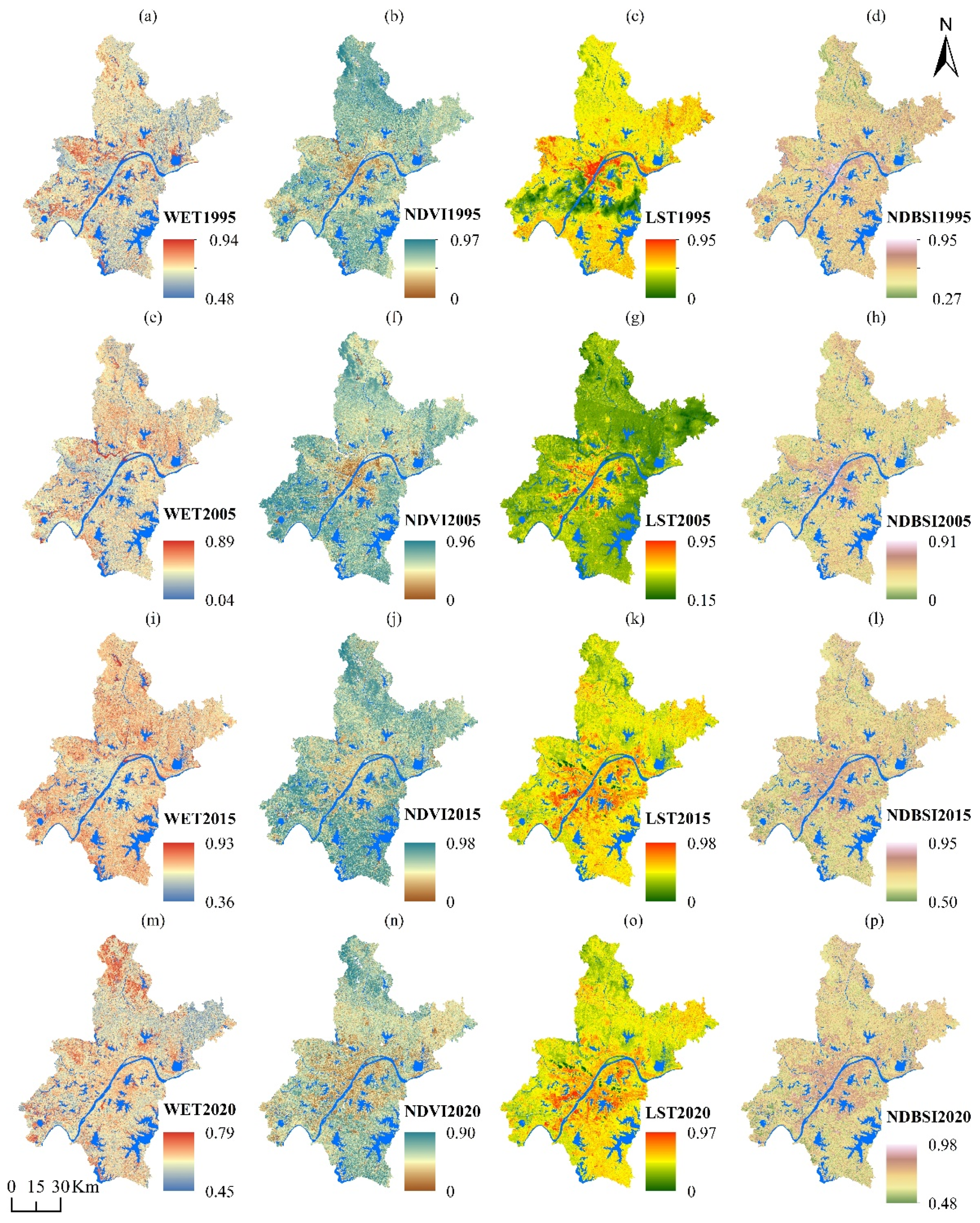
A comparison of the spatial distributions of the four ecological factors in the study area (Figure 3) shows high levels of land surface moisture close to and alongside the Yangtze River, which extends in the central part of Wuhan from west to east. The NDVI is high on the northeast side, along the Yangtze and Han rivers, the central part of Wuhan and in patches in the south and east. Comparing the NDVI, LST and moisture maps shows that moderate temperature and moisture are the most favorable conditions for vegetation growth, whereas extreme weather conditions can damage plant vitality. The temperature and moisture conditions are moderate in the study area and the NDVI is remarkably high. A high LST is detected in the southern part of Wuhan, with some patches in the north and east. A moderate LST is detected in the central part of Wuhan. The NDBSI does not display much variation, as most of the study area is covered by agricultural land (Figure 3).

To test the representativeness of the index IRSEI, we calculate the correlation coefficients among IRSEI, WET, NDVI, NDSI and LST in the same period (Table S1, Supplementary Materials), and test the applicability of the model through average correlations. From 1995 to 2015, the average correlation of IRSEI with the other variables is the highest, ranging from 0.60 to 0.70. The mean correlation of IRSEI over this period was 0.64, which indicates that IRSEI integrates most of the information embodied in all four indicators. It is more representative than any single indicator and can better reflect the ecological situation.

3.2. Spatial and Temporal Distribution of UEQ in Wuhan

Generally, higher IRSEI values are associated with higher levels of greenness and moisture, whereas lower IRSEI values are directly proportional to dryness and temperature. This implies that high IRSEI values represent positive ecological conditions.

As shown in Figure 4, the IRSEI increases from 0.79 to 0.98 from 2010 to 2015, indicating improved ecological conditions. However, from the second half of 2015 up to 2020, its value drops to 0.82, indicating deterioration. Comparing the values from 2010 to 2020 indicates overall improved conditions, as the IRSEI increases from 0.79 to 0.82. However, the maximum values (1.09, 1.03 and 0.96) decline continuously, indicating that high-quality IRSEI conditions are declining continuously. Further, low-quality IRSEI conditions improve in the first half of the study period (1995 to 2005); however, in the second half (2005 to 2020), these conditions decline and reach their previous stage. Our findings also show maximal variation in the median IRSEI values, i.e., indicating the recovery of favorable conditions (moderate to high temperature, moderate to low moisture and higher vegetation) for all factors during the study period.

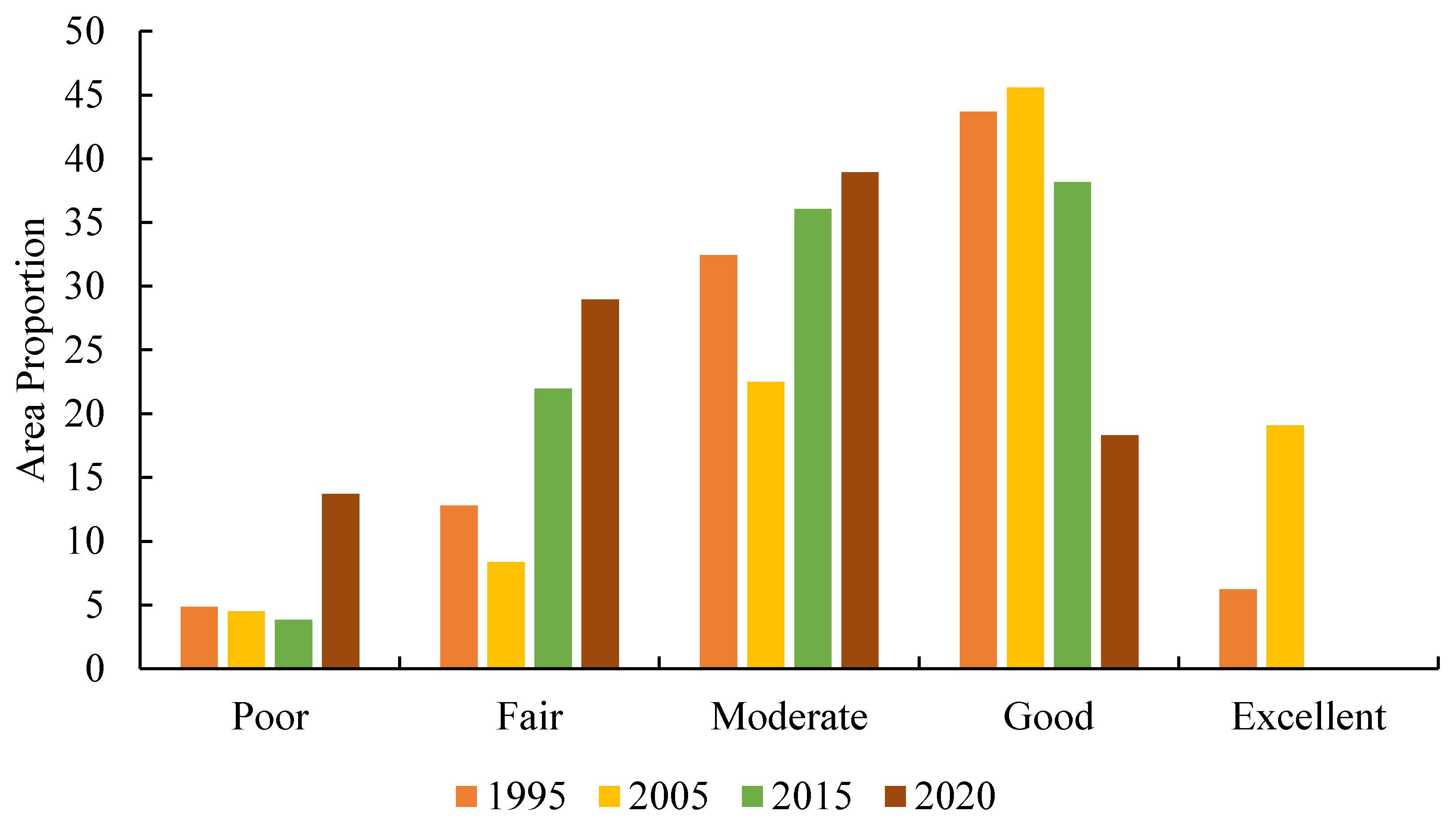
The mean IRSEI value and the area and percentage of each evaluation grade in Wuhan from 1995 to 2020 are displayed on Figure 4 and Figure 5. Overall, the proportion of areas with average and good IRSEI ratings is the highest during the study period (>57%). The proportions of average and above average regions are 82.33%, 87.14%, 74.21% and 57.34%, indicating that the ecological environment of Wuhan was unstable from 1995 to 2020, with ecological conditions first improving and subsequently deteriorating. The UEQ of the Xinzhou, Hanyang, Qiaokou, Huangpi and Caidian districts show the most obvious decline, with reduction rates of 32.32%, 30.18%, 27.84%, 27.67% and 27.24%, respectively.

From the perspective of a single year (see

Table 5. Area and proportion of the IRSEI over 1995 to 2020 in Wuhan city (unit: km², %).

IRSEI	1995		2005		2015		2020
	Area	Proportion	Area	Proportion	Area	Proportion	Area	Proportion
0–0.2	371	4.84%	344	4.49%	294	3.84%	1051	13.71%
0.2–0.4	981	12.80%	643	8.38%	1684	21.96%	2221	28.97%
0.4–0.6	2486	32.43%	1725	22.49%	2764	36.05%	2984	38.92%
0.6–0.8	3348	43.67%	3494	45.57%	2926	38.16%	1404	18.32%
0.8–1.0	478	6.23%	1463	19.08%	0	0.00%	8	0.10%

), the area share of good ecological environment in 1995 was the highest, reaching 43.67% of the total area. The area share of poor ecological environment was the lowest in 1995, comprising an area of only 371 km², or less than 5% of the total area. The share of poor ecological environment was approximately 12% of the total area. The area with a good ecological environment rating in 2005 was larger than that of 1995 and accounted for the highest proportion (45.57%), comprising an area of 3494 km². The percentage of area rated excellent was the smallest (6.23%) after 1995. In 2020, the poor ecological environment generally accounted for the highest proportion (38.92%), comprising an area of 2984 km². The good ecological environment rating accounted for only 18.32%.

The changing trend during the research period shows that the mean IRSEI values in 1995, 2005, 2015 and 2020 decreased year by year (0.60, 0.67, 0.58 and 0.47, respectively). The declining values indicate that the ecological environment of Wuhan has deteriorated continuously, probably owing to the rapid economic development of the city. According to the Wuhan Municipal Bureau of Statistics, the gross domestic product (GDP) increased from CNY 3.991 billion in 1978 to CNY 134.10 billion in 2017. The permanent resident population increased from 8.58 million people in 2004 to 10.33 million people in 2014. Ecological problems ascribed to human activities, such as vegetation damage and soil pollution, have become increasingly prominent.

As governments and social organizations have become increasingly aware of environmental protection, Wuhan has strengthened its enforcement of ecologically relevant laws and regulations, effectively halting the trend of environmental deterioration. This is reflected in the varying ecological evaluation grades. The differences in rating reflect an increase in area from 643 km² in 2005 to 1684 km² in 2015 (area expansion of 14%) to 2221 km² in 2020 (area expansion of 7%).

The spatial distribution (

Table 6. Area statistics of UEQ evaluation grade from 1995 to 2020 in Wuhan city (unit: km², %).

	IRSEI	1995		2005		2015		2020
		Area	Proportion	Area	Proportion	Area	Proportion	Area	Proportion
Caidian	0–0.2	33.34	3.41	44.30	4.53	43.34	4.43	159.00	16.25
	0.2–0.4	182.83	18.70	73.39	7.50	204.01	20.85	302.66	30.94
	0.4–0.6	318.68	32.59	115.98	11.86	301.04	30.77	356.95	36.49
	0.6–0.8	394.58	40.36	315.74	32.28	429.84	43.94	159.47	16.30
	0.8–1.0	48.29	4.94	428.85	43.84	0.03	0.00	0.26	0.03
Dongxihu	0–0.2	26.76	5.63	26.11	5.49	6.62	1.39	93.09	19.55
	0.2–0.4	107.11	22.52	58.36	12.26	161.61	33.96	160.44	33.70
	0.4–0.6	194.95	40.98	114.47	24.05	191.74	40.29	172.55	36.25
	0.6–0.8	144.37	30.35	176.46	37.08	115.93	24.36	49.77	10.45
	0.8–1.0	2.48	0.52	100.51	21.12	0.01	0.00	0.22	0.05
Hannan	0–0.2	12.66	4.91	9.69	3.76	13.55	5.26	42.96	16.68
	0.2–0.4	42.45	16.45	15.87	6.16	55.44	21.51	83.13	32.28
	0.4–0.6	111.99	43.40	31.36	12.17	88.47	34.33	97.70	37.93
	0.6–0.8	81.25	31.49	94.55	36.69	100.24	38.90	33.61	13.05
	0.8–1.0	9.70	3.76	106.23	41.22	0.00	0.00	0.17	0.07
Hanyang	0–0.2	9.14	9.17	11.42	11.46	5.12	5.14	31.27	31.40
	0.2–0.4	31.18	31.30	27.49	27.59	52.91	53.10	36.47	36.63
	0.4–0.6	35.36	35.48	27.14	27.24	28.77	28.87	24.28	24.39
	0.6–0.8	23.74	23.83	27.28	27.38	12.84	12.89	7.53	7.57
	0.8–1.0	0.22	0.22	6.30	6.32	0.00	0.00	0.01	0.01
Hongshan	0–0.2	42.60	8.93	41.29	8.66	24.48	5.13	104.50	21.91
	0.2–0.4	93.16	19.53	81.07	16.99	158.38	33.20	143.26	30.04
	0.4–0.6	184.41	38.66	129.99	27.25	159.77	33.49	147.52	30.93
	0.6–0.8	151.94	31.85	181.63	38.07	134.42	28.18	81.66	17.12
	0.8–1.0	4.88	1.02	43.07	9.03	0.01	0.00	0.02	0.01
Huangpi	0–0.2	77.87	3.67	63.18	2.97	86.94	4.09	216.05	10.17
	0.2–0.4	122.09	5.75	105.77	4.98	368.63	17.35	483.26	22.74
	0.4–0.6	488.82	23.02	595.10	28.01	865.43	40.74	960.08	45.19
	0.6–0.8	1187.44	55.92	1173.85	55.25	803.40	37.82	462.81	21.78
	0.8–1.0	247.18	11.64	186.56	8.78	0.07	0.00	2.57	0.12
Jiangan	0–0.2	17.08	23.72	16.66	23.21	2.93	4.08	22.01	30.71
	0.2–0.4	23.97	33.28	28.60	39.84	40.42	56.30	27.62	38.53
	0.4–0.6	20.21	28.06	18.12	25.23	22.22	30.95	16.14	22.51
	0.6–0.8	10.70	14.85	7.76	10.81	6.22	8.66	5.91	8.24
	0.8–1.0	0.06	0.09	0.65	0.91	0.00	0.00	0.00	0.00
Jianghan	0–0.2	9.42	34.28	9.08	33.07	1.13	4.10	10.69	38.95
	0.2–0.4	11.41	41.50	12.48	45.46	18.63	67.85	11.69	42.58
	0.4–0.6	4.84	17.60	4.16	15.16	6.54	23.83	4.17	15.20
	0.6–0.8	1.82	6.61	1.61	5.86	1.16	4.22	0.90	3.26
	0.8–1.0	0.00	0.01	0.12	0.45	0.00	0.00	0.00	0.00
Jiangxia	0–0.2	77.13	4.60	58.66	3.50	68.87	4.11	173.97	10.37
	0.2–0.4	153.61	9.16	92.52	5.52	285.30	17.01	368.37	21.96
	0.4–0.6	581.14	34.66	283.28	16.89	429.99	25.64	643.15	38.35
	0.6–0.8	757.98	45.21	806.03	48.06	892.77	53.23	487.53	29.07
	0.8–1.0	106.69	6.36	436.59	26.03	0.16	0.01	4.21	0.25
Qiaokou	0–0.2	6.98	18.06	8.96	23.25	1.63	4.23	14.54	37.70
	0.2–0.4	16.31	42.17	16.03	41.61	24.51	63.61	15.28	39.61
	0.4–0.6	8.19	21.19	8.91	23.13	10.09	26.20	7.36	19.08
	0.6–0.8	6.93	17.92	3.99	10.36	2.30	5.97	1.39	3.61
	0.8–1.0	0.25	0.66	0.64	1.66	0.00	0.00	0.00	0.00
Qingshan	0–0.2	10.40	20.39	8.53	16.66	1.58	3.09	15.73	30.69
	0.2–0.4	23.10	45.31	20.76	40.55	25.24	49.30	20.53	40.06
	0.4–0.6	12.99	25.47	15.01	29.32	18.78	36.68	11.98	23.37
	0.6–0.8	4.38	8.59	6.19	12.09	5.60	10.93	3.02	5.89
	0.8–1.0	0.12	0.24	0.71	1.39	0.00	0.00	0.00	0.00
Wuchang	0–0.2	10.64	20.73	11.20	21.70	3.01	5.83	13.72	26.48
	0.2–0.4	23.56	45.91	22.57	43.72	24.67	47.78	18.84	36.37
	0.4–0.6	10.70	20.85	10.82	20.97	16.45	31.86	12.13	23.41
	0.6–0.8	6.25	12.17	5.90	11.44	7.50	14.53	7.11	13.72
	0.8–1.0	0.18	0.35	1.12	2.18	0.00	0.00	0.00	0.01
Xinzhou	0–0.2	37.12	2.78	34.87	2.61	35.06	2.62	153.92	11.51
	0.2–0.4	150.44	11.26	87.89	6.57	264.28	19.76	549.54	41.09
	0.4–0.6	514.20	38.48	370.17	27.68	624.33	46.69	530.22	39.65
	0.6–0.8	577.11	43.18	692.87	51.82	413.46	30.92	103.51	7.74
	0.8–1.0	57.51	4.30	151.36	11.32	0.03	0.00	0.18	0.01

and Figure 6) shows that areas with a good ecological environment are distributed mainly in the surrounding urban areas of Wuhan. These areas have a relatively weak economy and the land-use types are mainly cultivated land and woodland, with rich vegetation and high biodiversity levels. The areas with poor ecological environments are concentrated in Hongshan, Hanyang, Wuchang and Qingshan. According to the different functions of each administrative region of Wuhan, Hongshan is based mainly on the education industry. Several colleges and universities are located in the area, and it is densely populated. Qingshan, Hanyang and Wuchang are primarily industrial areas. Heavy industrial companies, such as Wuhan Iron & Steel Co., Ltd., Wushi Chemical Co., Ltd. and Dongfeng Motor Co., Ltd., are located in these areas. Industrial production and human economic activities have a direct detrimental effect on the environment of these areas.

3.3. Dynamic Monitoring of UEQ in Wuhan

Based on the IRSEI grade classification, the detected changes were divided further into nine levels and seven classes. The range for the levels of detected changes was −4 to +4, with a positive value indicating that the UEQ had improved, 0 indicating no change and a negative value indicating deterioration. For the classes with no detected changes, level 0 was classified as unchanged, level −4 as significantly worse and levels −2 and −3 as worse; level −1 as slightly worse; level 1 as slightly better; levels 2 and 3 as better; and level 4 as significantly better (

Table 7. Change in the ecological index grade.

Change Grade	Level Change
Significantly worse	−4 (Excellent to Poor)
Obviously worse	−3 (Excellent to Fair/Good to Poor)
	−2 (Excellent to Moderate/Good to Fair/Moderate to Poor)
Slightly worse	−1 (Excellent to Good/Good to Moderate/Moderate to Fair/Fair to Poor)
No change	0 (no level change, eg. Excellent to Excellent)
Slightly better	1 (Above, and vice versa)
Obviously better	2 (Above, and vice versa)
	3 (Above, and vice versa)
Significantly better	4 (Above, and vice versa)

).

Table 8. Change in the ecological index grade from 1995 to 2020.

Change Grade	1995–2005		2005–2015		2015–2020
	Area	Percentage	Area	Percentage	Area	Percentage
Significantly worse	3	0.04%	20	0.26%	0	0.00%
Obviously worse	373	4.86%	1299	17.11%	981	12.85%
Slightly worse	1157	15.07%	2644	34.85%	2655	34.76%
No change	2952	38.45%	2634	34.70%	2984	39.08%
Slightly better	2165	28.20%	815	10.74%	816	10.69%
Obviously better	1008	13.13%	177	2.33%	199	2.61%
Significantly better	20	0.26%	0	0.00%	0	0.00%

presents the ecological changes in Wuhan from 1995 to 2020. The size of the area representing both UEQ and ecological deterioration (obviously worse and slightly worse) is 3636 km², accounting for the highest proportion (39.44%) over 2015–2020. The size of the area with the same UEQ (no change) is 2984 km², accounting for 35.56% of the total area. Among the areas with deteriorating UEQ, most (69.51%) deteriorated by one grade. Deterioration in UEQ accounted for 25.60%. Most of the areas showing improved environmental conditions improved by one grade, accounting for 79.41% of the entire improved area. The areas improving by two grades account for 18%. The areas representing levels 3 or 4 are relatively small, indicating gradual changes. The areas with significant changes are related to direct economic activities, such as the transformation of cultivated land and woodland into construction and industrial land. The spatial distribution of UEQ (Figure 7) shows that the deteriorating areas are located mainly around cities and most water bodies. The deterioration of the ecological environment around water bodies is related to a leakage of urban domestic sewage and enterprise wastewater and a rise in aquaculture in recent years. Moreover, the areas with a deteriorating ecological environment are expanding along both sides of the Yangtze and Han rivers. Except for the water area, the UEQ in the central metropolitan area remains mainly unchanged and several areas show signs of improvement. This result indicates that environmental governance in the main urban area of Wuhan has played a positive role in recent years.

3.4. Spatial Autocorrelation Analysis

We explore the spatial autocorrelation (SA) of the IRSEI at a grid cell scale of 500 m × 500 m and our results indicate the existence of SA. The Moran’s I was 0.568 in 1995, and 0.535 in 2020. All four IRSEI maps (1995, 2005, 2015 and 2020) display an extremely low probability (p-value < 0.01) of completely random spatial distribution. Therefore, the statistical significance test shows that SA exists for all of the ecological factors. The IRSEI increased in places where spatial distribution was favorable to the UEQ. In 1995, high-value clustering of the IRSEI in Wuhan was distributed mainly in the south and north of the study area, whereas low-value clustering was concentrated in the middle of the study area. In 2005, high IRSEI values started gathering gradually in the southern region, and low IRSEI values became more concentrated in the clustering distribution. By 2015, the high/high clustering and low/low clustering of the IRSEI in the study area became more dispersed and tended to spread in every direction. In 2020, low/low clusters had spread from the middle to the east and west, whereas high/high clusters were concentrated mainly in the south and north of Wuhan City.

The Moran’s I scatter graph is divided into four quadrants, corresponding to four different spatial distribution types (Figure 8). The first quadrant represents high/high clustering, the second quadrant low value and high-value aggregation, the third quadrant low/low aggregation and the fourth quadrant high-value and low-value aggregation. The IRSEI of Wuhan is concentrated mainly in the first and third quadrants. This result indicates that the IRSEI spatial distribution in Wuhan represents positive spatial autocorrelation, and high IRSEI agglomeration zones are mainly distributed in outer suburban areas, mainly in the north and southeast Wuhan.

4. Discussion

4.1. Literature, Policy and Practice

We have reviewed previous studies and demonstrated that it is feasible to evaluate the quality of the urban ecological environment through remote sensing. This research proposes a feasible method. Other remote sensing images could also have been used as data in this research, such as Tiangong-2 WIS images [11]. In terms of method improvement, we mainly improved the integration of quantitative factors. A related similar index, RSUSEI, has primarily increased remote sensing ecological factors by adding the impervious surface cover (ISC) [15]. ISC is also one of the most important factors that distinguish different types of land use/land cover characteristics in urban environments, and has a strong impact on UEQ. However, in our study we also consider the dryness index (NDBSI), the bare soil index (SI), the building index (IBI) and the normalized buildings–bare-soil index. However, there are strong correlations between the impervious surface, bare soil and building indices. Previous studies have found that the relationship between ISC and LST has the form of an exponential function, rather than a simple linear function, as commonly believed [43]. This exponential relationship has been confirmed by many subsequent studies [44,45]. Our IRSEI index takes into account the bare soil, building index and surface temperature. We suggest that the correlations of remote sensing ecological indicators affecting the regional ecological environment should be introduced into comprehensive indicators, or different indicators should be set according to the characteristics of the study region.

There are few high-quality ecological environment patches in Wuhan (IRSEI > 0.8), with close to zero over the past five years, and most of the patches are in the center of the ecological environment. Therefore, we propose a policy whereby Wuhan would focus on protecting forest land and gardens, build high-quality ecological corridors and coordinate the management of rivers in the future, so as to guide sustainable urban development and achieve sustainable development goals (such as SDG 11, sustainable cities and communities). Lake and wetland protection and ecological restoration and management will optimize the pattern of ecological security. Further analyses of the results indicate that there was a negative correlation between LSI, NDBSI and urban ecological quality. The ecological environment in areas with a high surface temperature, such as the Wuhan downtown area and coastal area around the Yangtze River, has tended to deteriorate; however, the humidity indices in these areas were also relatively high, which is conducive to ecological protection. Low vegetation index values in the central urban area also affect the quality of the ecological environment of Wuhan to a certain extent. The IRSEI can macro-evaluate the quality of the regional ecological environment, which is more convenient and efficient. In the future, higher precision can be introduced at the block level. Data, such as Google Street View data, could be used with machine learning algorithms to further identify the proportion of regional urban green space, trees, etc., and improve the accuracy of ecological environment assessment. The index has a high ability to distinguish between different land cover uses. The framework can also be easily extended to a global scale or to map other gridded socio-economic variables (such as GDP and population) to monitor and assess progress towards the SDGs [25]. The assessment and modelling of uses is critical to supporting sustainability assessment in achieving Sustainable Development Goals (SDGs), such as sustainable cities and communities. Therefore, IRSEI can be used to assess the spatial and temporal sustainability of cities.

4.2. Analysis of the Factors Affecting the UEQ

The regression least squares method (OLS) can be used to quantitatively describe the relationship between the ecological index and natural, economic and social factors in Wuhan. The data include temperature, precipitation, elevation, slope and DMSP as explanatory variables. The night light variable reflects the human footprint and fundamentally affects the urban ecological environment. Impervious surfaces and roads and a high population density are not conducive to UEQ. The regression coefficients represent the contribution of six independent variables to the dependent variable. The regression coefficients of precipitation and elevation are equal to 0.522 and 0.441, respectively, indicating that precipitation and elevation positively contribute to the IRSEI.

In contrast, the regression coefficients of night light and slope are negative, indicating that these variables contribute negatively to the IRSEI. The night light variable has a regression coefficient of –0.619, indicating a negative effect. The R² is 0.901 and p < 0.05, indicating that climate, precipitation, elevation, slope and night light data account for 90% of the variations of the IRSEI.

The regression equation between the IRSEI and the independent variables is as follows:

IRSEI = 0.926 + 0.148 × Temperature + 0.522 × Precipitation + 0.441 × Slope − 0.001 × Elevation − 0.619 × DMSP (R = 0.901).

4.3. Method Framework and Validation Analysis

Weighting is an important process in the development of aggregated ecological indices that help promote sustainability. Different weighting methods have different characteristics, and the method employed could reflect the subjectivity of the decision makers. However, such methods combined with remote sensing index data can facilitate decisions and reduce the calculations required.

PCA is widely used in the evaluation of the RSEI. In several studies, the three principal components obtained after dimensionality reduction did not show any obvious effects (contribution was below 15%). However, including all of the pixels in extensive data calculations is a time-consuming process. The RSEI employs a covariance-based (unstandardized) PCA to determine the importance of each indicator involved. The weight of each indicator can be assigned objectively and automatically based on the load (contribution) of each indicator to PC1. In this study, we used PCA and EW to comprehensively calculate the IRSEI. After improvement, the combined method was able to reflect the degree of change in the index, and the calculation was quick and uncomplicated. The spatial distribution of the UEQ over the study period (1995–2020) is consistent with the information in the bulletin on the eco-environmental situation in China in that year. The current, more popular assessment method is based on habitat quality (HQ) [46,47,48,49,50]. In further research, we intend to include HQ in this quantitative assessment.

4.4. Limitations and Future Prospects

The proposed UEQ evaluation model is feasible and straightforward, providing a new idea for ecological protection and comprehensively reflecting the changes in UEQ in Wuhan. From 1995 to 2020, the UEQ of Wuhan declined overall, probably owing to a combination of natural factors and human activities. However, the ecological level in the eastern and southeastern mountainous areas has increased because of the influence of forest resource protection, desertification land management and the warm and humid climate. In contrast, the regional ecological level has declined, owing to the overexploitation and overgrazing of lake resources in the northwest and southwest of Wuhan. The constantly rising levels of urbanization and construction over nearly 20 years have resulted in a downward trend in the UEQ. Overall, the ecology of Wuhan is in a fragile state. In 2020, the proportion of areas with poor ecological environment grades remained high, accounting for 42.68% of the total area.

In future social and economic development, we should follow the laws of nature, prioritize protection and rationally develop and utilize natural resources. The IRSEI effectively revealed the spatial distribution of and change in the UEQ in Wuhan, based on remote sensing images. Although four types of ecological factors closely related to the ecological environment were selected in the calculation process, the ecological environment is a complex and comprehensive variable. Areas with a deteriorating ecological environment tend to be spread along the Yangtze and Han rivers and around the central urban area. Urban expansion has damaged the ecological environment, and urban planning should integrate more ecological concepts to promote a harmonious coexistence and sustainable development for humans, nature and society.

Comprehensive quantitative evaluation requires selecting several impact factors that reflect the actual situation in the study area. We aimed to conduct the UEQ evaluation by employing a scientific, objective and feasible method. Nevertheless, choosing the UEQ evaluation index remains exploratory work. Determining the index weight affects the accuracy of the evaluation results. Accordingly, expanding research to a more scientific multifunction performance index system and determining the index weights require further work. Furthermore, the limited availability of data and a lack of longitudinal comparison of urban data have affected the scientific nature of our research results. In addition, our next step will be exploring how the IRSEI changes at different spatial scales. The rapid development of cities will inevitably lead to a series of ecological and environmental problems, and the deterioration of the ecological environment may further affect the surrounding environment, forming a cycle and harming urban sustainability. This study also demonstrates that IRSEI is characterized by spatial heterogeneity; that is, the poor UEQ patches will focus on areas where the ecological environment is poor and the urbanization is also highest.

5. Conclusions

In this study, the IRSEI model was used to evaluate and monitor the ecological environment in Wuhan from 1995 to 2020. The IRSEI is an ecological environmental quality assessment method based on remote sensing technology. The method has many advantages, such as the ease of obtaining parameters, a large time sequence span and a wide evaluation range. The UEQ method employing remote sensing technology is feasible and simple, and provides a new tool for territorial spatial control and spatiotemporal urban sustainable development. Our proposed UEQ assessment framework can also help to develop potentially relevant additional sub-indicators, which could help to address one of the current challenges in SDG monitoring, namely how to implement SDG indicators. We have implemented the proposed workflow in this study based on an open-source platform and free satellite data, making it an appealing option that is applicable in almost all countries.

The main conclusions from the results of this study are:

• The mean IRSEI value in Wuhan decreased annually from 2005 to 2015. The UEQ continued to decline, mainly because of the rapid economic development of Wuhan, reduction in vegetation coverage caused by human activities, gradual decrease in lake area and transformation of the land-use structure caused by urban expansion;
• From the perspective of spatial patterns, the UEQ of the central urban areas, such as Qingshan, Hanyang, Hongshan and Wuchang, was lower than that of the surrounding metropolitan areas, such as Huangpi, Jiangxia and Caidian. In terms of time series, the UEQ in the central city of Wuhan has been mainly unchanged or improved, indicating that the management of the ecological environment in the central city had achieved specific results;
• The global Moran’s I value range from 0.535 to 0.592 from 1995 to 2020, respectively, indicating that the IRSEI spatial distribution displays significant spatial heterogeneity. This finding indicates that high clustering gradually developed to the edge of the city, whereas low clustering gradually developed to the center of the city. The spatial correlation and local index cluster diagram of the IRSEI show that the high points are located mainly in the Huangpi and Jiangxia districts;
• The UEQ evaluation model constructed in this study is feasible and simple and could be implemented at no or negligible cost, making it applicable to most regional areas. Our model, therefore, could be considered a new tool for ecological management and protection, and for assessing progress toward urban sustainable development.

References

1. Van Tulder, R.; Rodrigues, S.B.; Mirza, H.; Sexsmith, K. The UN’s sustainable development goals: Can multinational enterprises lead the decade of action? J. Int. Bus. Policy 2021, 4, 1–21. [Google Scholar] [CrossRef]
2. Keeler, B.L.; Hamel, P.; McPhearson, T.; Hamann, M.H.; Donahue, M.L.; Meza Prado, K.A.; Arkema, K.K.; Bratman, G.N.; Brauman, K.A.; Finlay, J.C.; et al. Social-ecological and technological factors moderate the value of urban nature. Nat. Sustain. 2019, 2, 29–38. [Google Scholar] [CrossRef]
3. Elmqvist, T.; Andersson, E.; Frantzeskaki, N.; McPhearson, T.; Olsson, P.; Gaffney, O.; Takeuchi, K.; Folke, C. Sustainability and resilience for transformation in the urban century. Nat. Sustain. 2019, 2, 267–273. [Google Scholar] [CrossRef]
4. United Nations. 2018 Revision of World Urbanization Prospects. Available online: https://www.un.org/development/desa/publications/2018-revision-of-world-urbanization-prospects.html (accessed on 16 May 2018).
5. United Nations. Cities and Pollution. Available online: https://www.un.org/en/climatechange/climate-solutions/cities-pollution (accessed on 14 July 2020).
6. Worldbank. Urban Development. Available online: https://www.worldbank.org/en/topic/urbandevelopment/overview#1 (accessed on 20 April 2020).
7. Dale, V.H. The relationship between land-use change and climate change. Ecol. Applic. 1997, 7, 753–769. [Google Scholar] [CrossRef]
8. McDaniel, J.; Alley, K.D. Connecting local environmental knowledge and land use practices: A human ecosystem approach to urbanization in West Georgia. Urban Ecosys. 2005, 8, 23–38. [Google Scholar] [CrossRef]
9. de Andrés, M.; Barragán, J.M.; García Sanabria, J. Relationships between coastal urbanization and ecosystems in Spain. Cities 2017, 68, 8–17. [Google Scholar] [CrossRef]
10. Yang, C.; Zhang, C.; Li, Q.; Liu, H.; Gao, W.; Shi, T.; Liu, X.; Wu, G. Rapid urbanization and policy variation greatly drive ecological quality evolution in Guangdong-Hong Kong-Macau Greater Bay Area of China: A remote sensing perspective. Ecol. Indic. 2020, 115, 106373. [Google Scholar] [CrossRef]
11. Ariken, M.; Zhang, F.; Liu, K.; Fang, C.; Kung, H.-T. Coupling coordination analysis of urbanization and eco-environment in Yanqi Basin based on multi-source remote sensing data. Ecol. Indic. 2020, 114, 106331. [Google Scholar] [CrossRef]
12. Bonilla-Bedoya, S.; Mora, A.; Vaca, A.; Estrella, A.; Herrera, M.Á. Modelling the relationship between urban expansion processes and urban forest characteristics: An application to the Metropolitan District of Quito. Comput. Environ. Urban Syst. 2020, 79, 101420. [Google Scholar] [CrossRef]
13. Kerr, J.T.; Ostrovsky, M. From space to species: Ecological applications for remote sensing. Trends Ecol. Evol. 2003, 18, 299–305. [Google Scholar] [CrossRef]
14. Weber, T.; Sloan, A.; Wolf, J. Maryland’s Green Infrastructure Assessment: Development of a comprehensive approach to land conservation. Landsc. Urban Plan. 2006, 77, 94–110. [Google Scholar] [CrossRef]
15. Firozjaei, M.K.; Fathololoumi, S.; Weng, Q.; Kiavarz, M.; Alavipanah, S.K. Remotely sensed urban surface ecological index (RSUSEI): An analytical framework for assessing the surface ecological status in urban environments. Remote Sens. 2020, 12, 2029. [Google Scholar] [CrossRef]
16. Rapport, D.J.; Costanza, R.; McMichael, A.J. Assessing ecosystem health. Trends Ecol. Evol. 1998, 13, 397–402. [Google Scholar] [CrossRef]
17. Sfriso, A.; Facca, C.; Ghetti, P.F. Validation of the macrophyte quality index (MaQI) set up to assess the ecological status of italian marine transitional environments. Hydrobiologia 2009, 617, 117–141. [Google Scholar] [CrossRef]
18. Hu, X.; Xu, H. A new remote sensing index for assessing the spatial heterogeneity in urban ecological quality: A case from Fuzhou City, China. Ecol. Indic. 2018, 89, 11–21. [Google Scholar] [CrossRef]
19. Shan, W.; Jin, X.; Ren, J.; Wang, Y.; Xu, Z.; Fan, Y.; Gu, Z.; Hong, C.; Lin, J.; Zhou, Y. Ecological environment quality assessment based on remote sensing data for land consolidation. J. Clean. Prod. 2019, 239, 118126. [Google Scholar] [CrossRef]
20. Cai, B.; Shao, Z.; Fang, S.; Huang, X.; Huq, M.E.; Tang, Y.; Li, Y.; Zhuang, Q. Finer-scale spatiotemporal coupling coordination model between socioeconomic activity and eco-environment: A case study of Beijing, China. Ecol. Indic. 2021, 131, 108165. [Google Scholar] [CrossRef]
21. Yue, H.; Liu, Y.; Li, Y.; Lu, Y. Eco-environmental quality assessment in china’s 35 major cities based on remote sensing ecological index. IEEE Access 2019, 7, 51295–51311. [Google Scholar] [CrossRef]
22. Liao, W.; Jiang, W. Evaluation of the Spatiotemporal Variations in the Eco-environmental Quality in China Based on the Remote Sensing Ecological Index. Remote Sens. 2020, 12, 2462. [Google Scholar] [CrossRef]
23. Wang, J.; Liu, D.; Ma, J.; Cheng, Y.; Wang, L. Development of a large-scale remote sensing ecological index in arid areas and its application in the Aral Sea Basin. J. Arid Land 2021, 13, 40–55. [Google Scholar] [CrossRef]
24. Xu, H.; Wang, Y.; Guan, H.; Shi, T.; Hu, X. Detecting ecological changes with a remote sensing based ecological index (RSEI) produced time series and change vector analysis. Remote Sens. 2019, 11, 2345. [Google Scholar] [CrossRef] [Green Version]
25. Estoque, R.C. A Review of the Sustainability Concept and the State of SDG Monitoring Using Remote Sensing. Remote Sens. 2020, 12, 1770. [Google Scholar] [CrossRef]
26. Collins, J.B.; Woodcock, C.E. An assessment of several linear change detection techniques for mapping forest mortality using multitemporal landsat TM data. Remote Sens. Environ. 1996, 56, 66–77. [Google Scholar] [CrossRef]
27. Yarbrough, L.D.; Easson, G.; Kuszmaul, J.S. Proposed workflow for improved Kauth–Thomas transform derivations. Remote Sens. Environ. 2012, 124, 810–818. [Google Scholar] [CrossRef]
28. Huang, C.; Wylie, B.; Yang, L.; Homer, C.; Zylstra, G. Derivation of a tasselled cap transformation based on Landsat 7 at-satellite reflectance. Int. J. Remote Sens. 2002, 23, 1741–1748. [Google Scholar] [CrossRef]
29. Xu, H.; Wang, M.; Shi, T.; Guan, H.; Fang, C.; Lin, Z. Prediction of ecological effects of potential population and impervious surface increases using a remote sensing based ecological index (RSEI). Ecol. Indic. 2018, 93, 730–740. [Google Scholar] [CrossRef]
30. Robinson, N.P.; Allred, B.W.; Jones, M.O.; Moreno, A.; Kimball, J.S.; Naugle, D.E.; Erickson, T.A.; Richardson, A.D. A dynamic landsat derived normalized difference vegetation index (NDVI) product for the conterminous united states. Remote Sens. 2017, 9, 863. [Google Scholar] [CrossRef] [Green Version]
31. Townshend, J.R.G.; Justice, C.O. Analysis of the dynamics of African vegetation using the normalized difference vegetation index. Int. J. Remote Sens. 1986, 7, 1435–1445. [Google Scholar] [CrossRef]
32. Sobrino, J.A.; Jiménez-Muñoz, J.C.; Paolini, L. Land surface temperature retrieval from LANDSAT TM 5. Remote Sens. Environ. 2004, 90, 434–440. [Google Scholar] [CrossRef]
33. Estoque, R.C.; Murayama, Y.; Myint, S.W. Effects of landscape composition and pattern on land surface temperature: An urban heat island study in the megacities of Southeast Asia. Sci. Total Environ. 2017, 577, 349–359. [Google Scholar] [CrossRef] [PubMed]
34. Artis, D.A.; Carnahan, W.H. Survey of emissivity variability in thermography of urban areas. Remote Sens. Environ. 1982, 12, 313–329. [Google Scholar] [CrossRef]
35. Min, M.; Lin, C.; Duan, X.; Jin, Z.; Zhang, L. Spatial distribution and driving force analysis of urban heat island effect based on raster data: A case study of the Nanjing metropolitan area, China. Sustain. Cities Soc. 2019, 50, 101637. [Google Scholar] [CrossRef]
36. Carlson, T.N.; Ripley, D.A. On the relation between NDVI, fractional vegetation cover, and leaf area index. Remote Sens. Environ. 1997, 62, 241–252. [Google Scholar] [CrossRef]
37. Kerr, Y.H.; Lagouarde, J.P.; Imbernon, J. Accurate land surface temperature retrieval from AVHRR data with use of an improved split window algorithm. Remote Sens. Environ. 1992, 41, 197–209. [Google Scholar] [CrossRef]
38. Amiri, V.; Rezaei, M.; Sohrabi, N. Groundwater quality assessment using entropy weighted water quality index (EWQI) in Lenjanat, Iran. Environ. Earth Sci. 2014, 72, 3479–3490. [Google Scholar] [CrossRef]
39. Liu, G.-X.; Wu, M.; Jia, F.-R.; Yue, Q.; Wang, H.-M. Entropy-weighted comprehensive evaluation of petroleum flow in China during 1980–2015. J. Cleaner Prod. 2018, 195, 593–604. [Google Scholar] [CrossRef]
40. Islam, A.R.M.T.; Al Mamun, A.; Rahman, M.M.; Zahid, A. Simultaneous comparison of modified-integrated water quality and entropy weighted indices: Implication for safe drinking water in the coastal region of Bangladesh. Ecol. Indic. 2020, 113, 106229. [Google Scholar] [CrossRef]
41. Yang, J.Y.; Wu, T.; Pan, X.Y.; Du, H.T.; Li, J.L.; Zhang, L.; Men, M.X.; Chen, Y. Ecological quality assessment of Xiongan New Area based on remote sensing ecological index. J. Appl. Ecol. 2019, 30, 277–284. [Google Scholar] [CrossRef]
42. Overmars, K.d.; De Koning, G.; Veldkamp, A. Spatial autocorrelation in multi-scale land use models. Ecol. Modell. 2003, 164, 257–270. [Google Scholar] [CrossRef]
43. Xu, H. Analysis of impervious surface and its impact on urban heat environment using the normalized difference impervious surface index (NDISI). Photogramm. Eng. Remote Sens. 2010, 76, 557–565. [Google Scholar] [CrossRef]
44. Meng, F.; Shan, B.; Liu, M. Remote-sensing evaluation of the relationship between urban heat islands and urban biophysical descriptors in Jinan, China. J. Appl. Remote Sens. 2014, 8, 083693. [Google Scholar] [CrossRef]
45. Balçik, F.B. Determining the impact of urban components on land surface temperature of Istanbul by using remote sensing indices. Environ. Monit. Assess. 2014, 186, 859–872. [Google Scholar] [CrossRef]
46. Chen, T.; Hui, E.C.M.; Wu, J.; Lang, W.; Li, X. Identifying urban spatial structure and urban vibrancy in highly dense cities using georeferenced social media data. Habitat Int. 2019, 89, 102005. [Google Scholar] [CrossRef]
47. Li, F.; Wang, L.; Chen, Z.; Clarke, K.C.; Li, M.; Jiang, P. Extending the SLEUTH model to integrate habitat quality into urban growth simulation. J. Environ. Manag. 2018, 217, 486–498. [Google Scholar] [CrossRef] [Green Version]
48. Liu, J.; Zhang, G.; Zhuang, Z.; Cheng, Q.; Gao, Y.; Chen, T.; Huang, Q.; Xu, L.; Chen, D. A new perspective for urban development boundary delineation based on SLEUTH-InVEST model. Habitat Int. 2017, 70, 13–23. [Google Scholar] [CrossRef]
49. Romero-Calcerrada, R.; Luque, S. Habitat quality assessment using Weights-of-Evidence based GIS modelling: The case of Picoides tridactylus as species indicator of the biodiversity value of the Finnish forest. Ecol. Modell. 2006, 196, 62–76. [Google Scholar] [CrossRef]
50. Terrado, M.; Sabater, S.; Chaplin-Kramer, B.; Mandle, L.; Ziv, G.; Acuña, V. Model development for the assessment of terrestrial and aquatic habitat quality in conservation planning. Sci. Total Environ. 2016, 540, 63–70. [Google Scholar] [CrossRef] [PubMed] [Green Version]
Figure 1. Location of Wuhan city.
Remotesensing 13 04440 g001
Figure 2. Overall methodological framework.
Remotesensing 13 04440 g002
Figure 3. Spatial distribution of ecological indicators, 1995–2020. (ad) indicators 1995, (eh) indicators 2005, (il) indicators 2015, (mp) indicators 2020.
Remotesensing 13 04440 g003
Figure 4. Changing trend of the IRSEI in each district of Wuhan from 1995 to 2020.
Remotesensing 13 04440 g004
Figure 5. Changing area proportion of the IRSEI in Wuhan from 1995 to 2020.
Remotesensing 13 04440 g005
Figure 6. Grading map of UEQ from 1995 to 2020 in Wuhan city. (a) IRSEI 1995, (b) IRSEI 2005, (c) IRSEI 2015 and (d) IRSEI 2020.
Remotesensing 13 04440 g006
Figure 7. Spatial transfer distributions of the ecological levels of the IRSEI in Wuhan from 1995 to 2020.
Remotesensing 13 04440 g007
Figure 8. Spatial correlation and Moran index scatterplot of IRSEI from 1995 to 2020 in Wuhan city. (a) SA with 1995, (b) SA with 2005, (c) SA with 2015 and (d) SA with 2020. (Note: SA—Spatial autocorrelation).
Remotesensing 13 04440 g008