Article

Spaceborne GNSS-R for Sea Ice Classification Using Machine Learning Classifiers

1
College of Civil Engineering, Hefei University of Technology, Hefei 230009, China
2
Anhui Key Laboratory of Civil Engineering Structures and Materials, Hefei 230009, China
3
State Key Laboratory of Information Engineering in Surveying, Mapping and Remote Sensing, Wuhan University, Wuhan 430079, China
4
School of Environment Science and Spatial Informatics, China University of Mining and Technology, Xuzhou 221116, China
5
German Aerospace Center DLR, Institute for Solar-Terrestrial Physics, 17235 Neustrelitz, Germany
6
German Research Center for Geosciences GFZ, 14473 Potsdam, Germany
7
Institute of Geodesy and Geoinformation Science, Technische Universität Berlin, 10623 Berlin, Germany
*
Author to whom correspondence should be addressed.
Remote Sens. 2021, 13(22), 4577; https://0-doi-org.brum.beds.ac.uk/10.3390/rs13224577
Submission received: 11 September 2021 / Revised: 27 October 2021 / Accepted: 6 November 2021 / Published: 14 November 2021
(This article belongs to the Special Issue Recent Advances in GNSS Reflectometry)

Abstract

:
The knowledge of Arctic Sea ice coverage is of particular importance in studies of climate change. This study develops a new sea ice classification approach based on machine learning (ML) classifiers through analyzing spaceborne GNSS-R features derived from the TechDemoSat-1 (TDS-1) data collected over open water (OW), first-year ice (FYI), and multi-year ice (MYI). A total of eight features extracted from GNSS-R observables collected in five months are applied to classify OW, FYI, and MYI using the ML classifiers of random forest (RF) and support vector machine (SVM) in a two-step strategy. Firstly, randomly selected 30% of samples of the whole dataset are used as a training set to build classifiers for discriminating OW from sea ice. The performance is evaluated using the remaining 70% of samples through validating with the sea ice type from the Special Sensor Microwave Imager Sounder (SSMIS) data provided by the Ocean and Sea Ice Satellite Application Facility (OSISAF). The overall accuracy of RF and SVM classifiers are 98.83% and 98.60% respectively for distinguishing OW from sea ice. Then, samples of sea ice, including FYI and MYI, are randomly split into training and test dataset. The features of the training set are used as input variables to train the FYI-MYI classifiers, which achieve an overall accuracy of 84.82% and 71.71% respectively by RF and SVM classifiers. Finally, the features in every month are used as training and testing set in turn to cross-validate the performance of the proposed classifier. The results indicate the strong sensitivity of GNSS signals to sea ice types and the great potential of ML classifiers for GNSS-R applications.

1. Introduction

Arctic sea ice is one of the most significant components in studies of climate change [1]. The knowledge of sea ice information is useful for shipping route planning and offshore oil/gas exploration. As one of the most important sea ice parameters, sea ice type is of particular interest since the characteristics of first-year ice (FYI) and multi-year ice (MYI) are different [2]. Compared to FYI, MYI has greater thickness and higher albedo, which is critical for energy exchange in the air-sea interface. Some previous studies indicated that the Arctic sea ice has reduced in extent and a part of ice cover is becoming thinner, changing from thicker MYI to thinner FYI [3]. The surface roughness and dielectric constant of different sea ice types change at different stages of ice growth. It is well known that the surface of FYI is usually smoother than that of MYI. In addition, the salinity of FYI is higher than that of MYI. The FYI around the floe edges tends to undergo deformation when it collides with thicker ice. In general, the ice that survives at least one summer is regarded as MYI, which retains low salinity values and an undulating surface. These characteristics of different sea ice types are the basis for classification.
A wide variety of techniques has been applied to characterize changes in sea ice. Sea ice can be monitored from different platforms, such as buoys [4], ships [5], aircraft [6], and satellites [7]. Among them, satellite-based microwave remote sensing has been regarded as the most effective tool for monitoring sea ice [7].
In recent years, Global Navigation Satellite System (GNSS) Reflectometry (GNSS-R) has emerged as a powerful tool for sensing bio-geophysical features using L-band signals scattered from the Earth’s surface [8]. GNSS-R was initially proposed for ocean altimetry in 1993 [9] after the concept of GNSS-R was proposed in 1988 [10]. Subsequently, the scope of the applications of GNSS-R has been extended to various fields, such as wind speed retrieval [11], snow depth estimation [12], soil moisture sensing [13], ocean altimetry [14], and sea ice detection [15]. Most GNSS-R studies were carried out using reflected L-band data collected on ground-based, airborne, and spaceborne platforms, and the latter one is regarded as the future trend due to its global coverage and high mobility [16]. The United-Kingdom (UK) TechDemoSat-1 [16] and NASA Cyclone GNSS (CYGNSS) [17], launched in 2014 and 2016 respectively, have promoted the research of spaceborne GNSS-R since their data are publicly available. Particularly, the TDS-1 data can be used for polar research as its global coverage, while the CYGNSS can only be applied in middle and lower latitude regions as its coverage of interest is the oceans within the latitude of ± 38°. Recently, some other spaceborne GNSS-R missions have been successfully carried out one after another, such as the Chinese BuFeng-1 A/B [18], and Fengyun 3E [19].
Many applications of GNSS-R make use of the specular scattering geometry since GNSS signals reflected from the Earth’s surface have the greatest amplitude at specular scattering. The Delay-Doppler Map (DDM), which is one of the most important GNSS-R observables, demonstrates the power scattering from the reflected surface as a function of time delays and Doppler shifts (Figure 1). The reflection over rough surfaces, such as open water (OW), is usually regarded as incoherent, which results in a “horseshoe” shape of DDM presented in Figure 1a. The specular scattering is considered coherent when the reflected surface is relatively smooth. The typical coherent DDM is shown in Figure 1b.
The TDS-1 data have been successfully used to sense sea ice parameters over the past few years. Yan et al. [20] firstly explored the sensitivity of TDS-1 Delay-Doppler Map (DDM) to sea ice presence using the pixel number of DDM with a signal-to-noise ratio (SNR) above a threshold. Similarly, Zhu et al. [21] proposed a differential DDM observable, which was used to recognize ice-water, water-water, water-ice, and ice-ice transitions. Schiavulli et al. [22] reconstructed a radar image based on DDM to distinguish sea ice from water. Alonso-Arroyo et al. [15] applied a matched filter ice detection approach with a probability of detection of 98.5%, a probability of false alarm of 3.6%, and a probability of error of 2.5%. Afterward, another study has proven that spaceborne GNSS-R can be effective for sea ice discrimination with a success rate of up to 98.22% compared to collocated passive microwave sea ice data [23]. Cartwright et al. [24] combined two features extracted from DDMs to detect sea ice with an agreement of 98.4% and 96.6% in the Antarctic and Arctic regions by comparing with the European Space Agency Climate Change Initiative sea ice concentration product. On the other hand, TDS-1 data were expanded to altimetry applications [25,26]. The ice sheet melt was also investigated in [27] using TDS-1 data. Furthermore, it has been shown that spaceborne GNSS-R is also useful for retrieving sea ice thickness [28], sea ice concentration [29], and sea ice type [30]. The GNSS-R observables derived from DDMs were used to classify Arctic sea ice in [30], where the TDS-1 sea ice types were compared with the sea ice type maps derived from Synthetic Aperture Radar (SAR) measurements.
In recent years, machine learning (ML) based methods have been widely used in geosciences and remote sensing applications [31]. ML has been proven powerful for applications in various remote sensing fields, such as classification [32,33], object detection [34], and parameter estimates [35]. Yan et al. [36] firstly adopted the neural network (NN) method to detect sea ice using spaceborne GNSS-R DDMs from TDS-1. This study demonstrated the potential of an NN-based approach for sea ice detection and sea ice concentration (SIC) estimation, which was further explored through the convolutional neural network (CNN) algorithm [37]. The DDMs were directly used as input variables in the CNN-based approach. Compared to NN and CNN, support vector machine (SVM) achieved the best performance in sea ice detection [38]. These three studies utilized the original DDM and the values derived from DDMs as input features for sensing sea ice. Zhu et al. [39] employed feature sequences that depict the characteristics of DDMs as input parameters to monitor sea ice using the decision tree (DT) and random forest (RF) algorithms. The RF aided method can discriminate sea ice from water with a success rate up to 98.03% validated with the collocated sea ice edge maps from the special sensor microwave imager sounder (SSMIS) data provided by the Ocean and Sea Ice Satellite Application Facility (OSISAF). Llaveria et al. [40] applied the NN algorithm for sea ice concentration and sea ice extent sensing using GNSS-R data from the FFSCat mission [40]. Rodriguez-Alvarez et al. [30] initially exploited the implementation of the classification and regression tree (CART) algorithm for sea ice classification using GNSS-R observables derived from GNSS-R DDM. The results showed that the FYI and MYI can be classified with an accuracy of 70% and 82.34% respectively. In order to illustrate the ML for sea ice sensing based on GNSS-R, relevant information about the above-mentioned studies is presented in Table 1.
As one of the most powerful ML algorithms, RF has been widely applied for remote sensing image classification [33,42,43]. However, RF has not been considered for classifying FYI and MYI using spaceborne GNSS-R data. In addition, the SVM-based method showed great potential in sea ice detection and classification in some previous studies [33,38]. Although SVM has been applied to sea ice classification using SAR images [33], the application of SVM to GNSS-R sea ice classification has not been investigated. Therefore, RF and SVM classifiers are adopted in this study to develop algorithms for sea ice classification. The purpose of this research is to demonstrate the feasibility of spaceborne GNSS-R to classify sea ice types using ML classifiers.
The spaceborne GNSS-R dataset and reference sea ice type data from the European Organization for the Exploitation of Meteorological Satellites (EUMETSAT) OSISAF [44] used in this study is firstly described in Section 2. Then, the theoretical basis and the proposed method for sea ice classification are described with details in Section 3. The sea ice classification results are presented in Section 4 and discussed in Section 5. The conclusions are finally addressed in Section 6.

2. Dataset Description

2.1. TDS-1 Mission and Dataset

The TDS-1 satellite began its data acquisition in September 2014 after its launch in July 2014. As one of eight instruments placed on the TDS-1 satellite, the Space GNSS Receiver-Remote Sensing Instrument (SGR-ReSI) was turned on only two days of an eight-day cycle until January 2018 [45]. The SGR-ReSI started its full-time operation in February 2018, and it came to the end in December 2018. The TDS-1 has provided a large amount of data at a global scale as the satellite runs on a quasi-Sun synchronous orbit with an inclination of 98.4°. Currently, the TDS-1 data are freely available on the Measurement of Earth Reflected Radio-navigation Signals by Satellite (MERRBYS) website (www.merrbys.co.uk, accessed on 11 September 2021). The TDS-1 data are processed into three levels, including Level 0 (L0), Level 1 (L1), and Level 2 (L2). Among them, L1 data are usually adopted in scientific research. L0 refers to the raw data, which are not accessible except for a small amount of sample data. L2 includes wind speed, mean square slope, and sea ice products. One of the most important GNSS-R observables is DDM, which is generated by the SGR-ReSI through the cross-correlation between scattered signals and locally generated code replicas with different delays and Doppler shifts. The orbit and instrument specifications of the TDS-1 mission are presented in Table 2 [45].

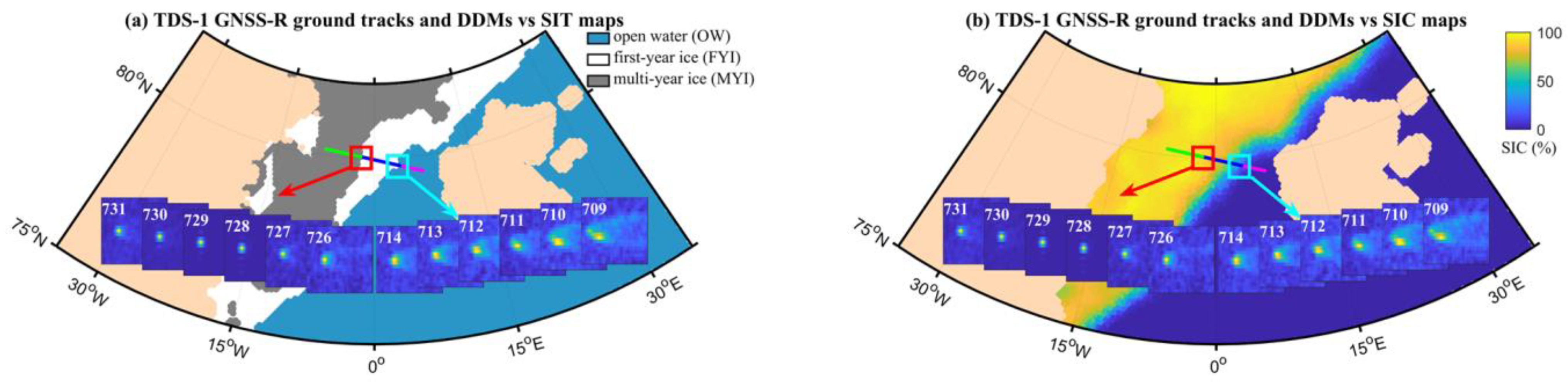
2.2. Reference Sea Ice Data

The sea ice type (SIT) provided by the OSISAF [44] is adopted as the reference data to train the sea ice classification model and validate the results. The OSISAF provides daily SIT maps with a spatial resolution of 10 km in the polar stereographic projection. The SIT products discriminate OW, FYI, and MYI through analyzing multi-sensor data. The data with a confidence level above 3 are adopted to avoid using low-quality data [44]. In addition, the SIC products generated from the SSMIS measurements provided by OSISAF are also used as reference data to analyze the impacts of SIC on sea ice classification. The reference SIC products are mapped on a grid with a size of 10 km × 10 km in the polar stereographic projection. The TDS-1 data is matched with the SIC maps through the SP location and data collection date, which are available in the TDS-1 dataset.
Figure 2a presents the GNSS-R ground tracks over OW, FYI, and MYI on 26 November 2015. The TDS-1 DDMs over OW-FYI and FYI-MYI transitions are shown in the figure. Meanwhile, the GNSS-R ground tracks are mapped against the SIC map in Figure 2b. In general, the SIC of MYI is higher than that of FYI.

3. Theory and Methods

3.1. Spaceborne GNSS-R Features

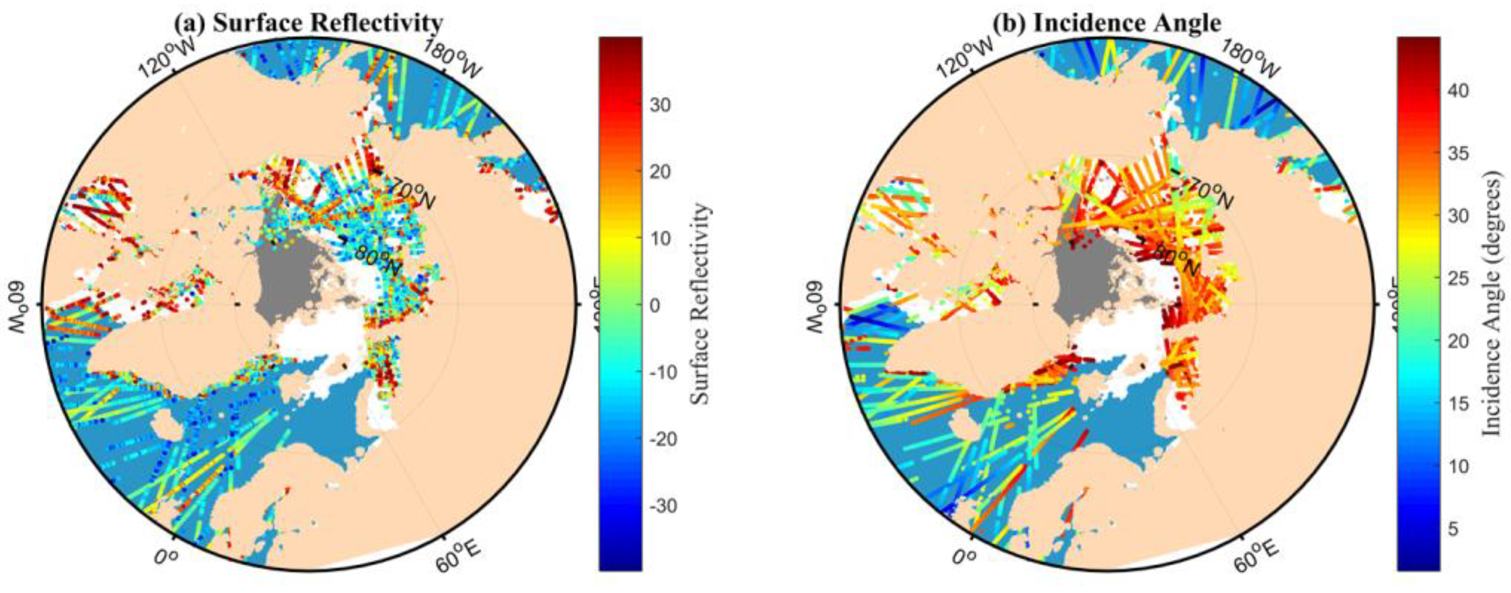
3.1.1. Surface Reflectivity

The GNSS-R instrument (e.g., SGR-ReSI) receives signals directly transmitted from GNSS constellations and scattered from the Earth’s surface. For the TDS-1 mission, the signals observed are the L1 C/A codes with a center frequency of 1.575 GHz. The L-band signal is useful for remote sensing applications due to its insensitivity to the precipitation and atmosphere. The specular reflections are dominant when the surface is relatively flat and smooth. As demonstrated in [15], the GNSS-R signal received over sea ice is usually coherent due to its smooth surface. Thus, the coherent surface reflectivity S R c o h at the specular point (SP) can be modeled as [46,47],
S R c o h = ( 4 π ) 2 ( R t + R r ) 2 ( λ ) 2 G r G t P t P c o h ,
where P c o h is the coherently received power reflected by the surface, R r and R t are the distances from the receiver and transmitter to the SP respectively, G r and G t are the antenna gain of the receiver and transmitter, λ is the GNSS signal wavelength, and P t is the power transmitted by GNSS satellites.
Most of the variables in (1) can be obtained from the TDS-1 L1b data. R r and R t can be easily calculated according to the positions of the transmitter, receiver, and SP, which are stored in the metadata. G r at SP can be directly extracted from the metadata. The noise floor is determined using the average value of the first four rows of DDM [23]. The transmitted signal power can be derived using [48],
P t G t = 4 π R d 2 G d P d ,  
where P t G t is also termed as effective isotropic radiated power (EIRP). P d is the direct power, R d is the distance from the transmitter to receiver, and G d is the zenith antenna gain, which is set as 4 dB in this study according to the Merrbys documentation [45,49].
As demonstrated in [28], the received power originates from a region surrounding the SP, which is usually the first Fresnel zone. As demonstrated in [50], the Fresnel reflectivity S R c o h can also be modeled as,
S R c o h = | R | 2 · e x p [ ( 4 π λ c o s θ i σ ) 2 ] ,  
where θ i stands for the incidence angle and σ is the surface root mean square (RMS) height. The second term in Equation (3) represents the surface roughness. The R represents the Fresnel reflection coefficient, which can be derived through Equations (4)–(6):
R = 1 2 ( R V V R H H ) ,
R V V = ϵ i c o s θ i ϵ i s i n 2 θ i ϵ i c o s θ i + ϵ i s i n 2 θ i ,  
R H H = c o s θ i ϵ i s i n 2 θ i c o s θ i + ϵ i s i n 2 θ i ,  
where θ i is the incidence angle over the sea ice, and ϵ i is the permittivity of sea ice, which is related to sea ice types. In this study, the data with an incidence angle below 45° are applied. Data marked by the quality flags eclipse or direct signal in DDM [51] have also been removed to deal with reliable data. The TDS-1 surface reflectivity and corresponding incidence angle distribution in Arctic regions in 5 days (from 11 to 15 February 2018) is presented in Figure 3.

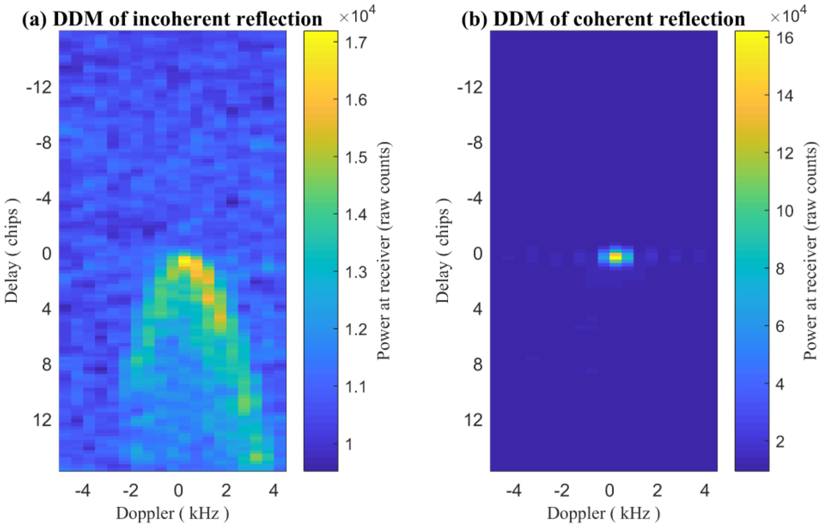
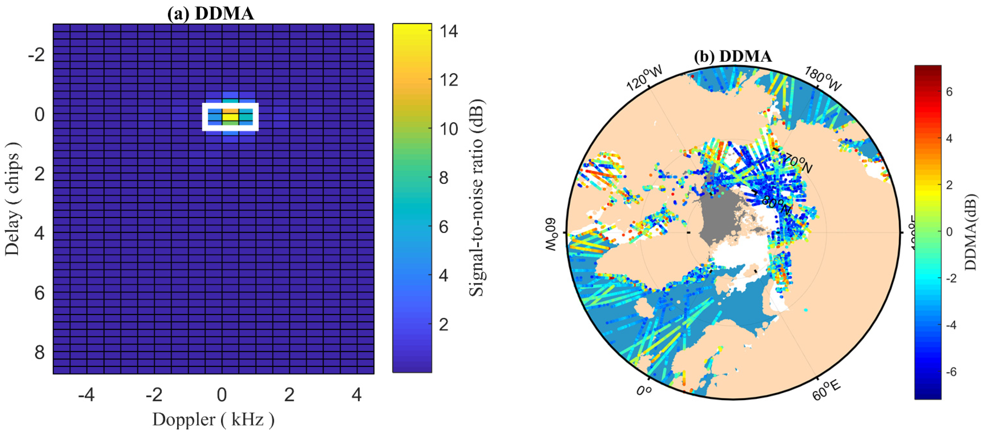
3.1.2. Features Derived from DDM

Besides the surface reflectivity, the other seven GNSS-R observables are chosen for sea ice classification. GNSS-R observables are defined as characteristics derived from the DDMs that describe their power and shape.
The DDM average (DDMA), which represents the mean signal-to-noise ratio (SNR) values over the point of peak SNR (Figure 4a), is applied in this study to classify sea ice types. As shown in Figure 4a, the DDMA expands 3 delay bins and 3 Doppler shifts centered at the peak SNR point. The distribution of DDMA in 5 days (from 11 to 15 February 2018) is presented in Figure 4b compared with the OSISAF SIT map.
As illustrated in [23,39], the integrated delay waveform (IDW) is defined as the summation of 20 delay waveforms, which are the cross-sections of DDM at 20 different Doppler shifts. The cross-section of zero Doppler shift is defined as the central delay waveform (CDW) of the DDM. The degree of difference between IDW and CDW is described by differential delay waveform (DDW), which is depicted as follows,
DDW = NIDW NCDW ,  
where NIDW and NCDW represent the normalized IDW and CDW respectively. The NIDW is related to the power spreading characteristics caused by surface roughness. The delay waveforms from delay bins −5 to 20 over OW, FYI, and MYI surfaces are shown in Figure 5.
Features extracted from delay waveforms are described as follows:
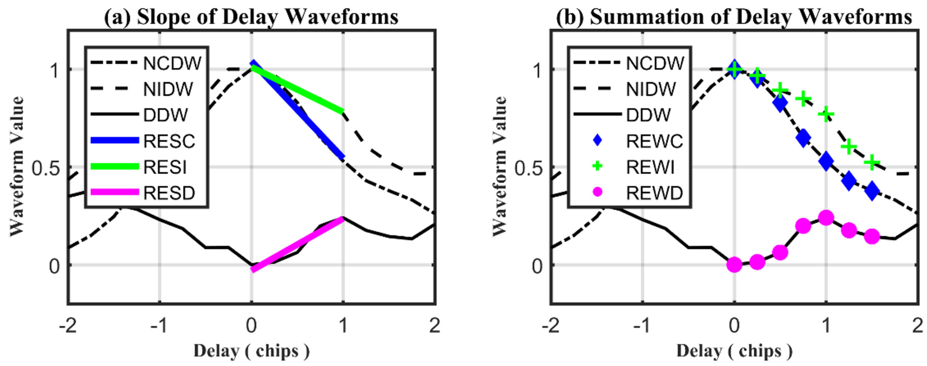
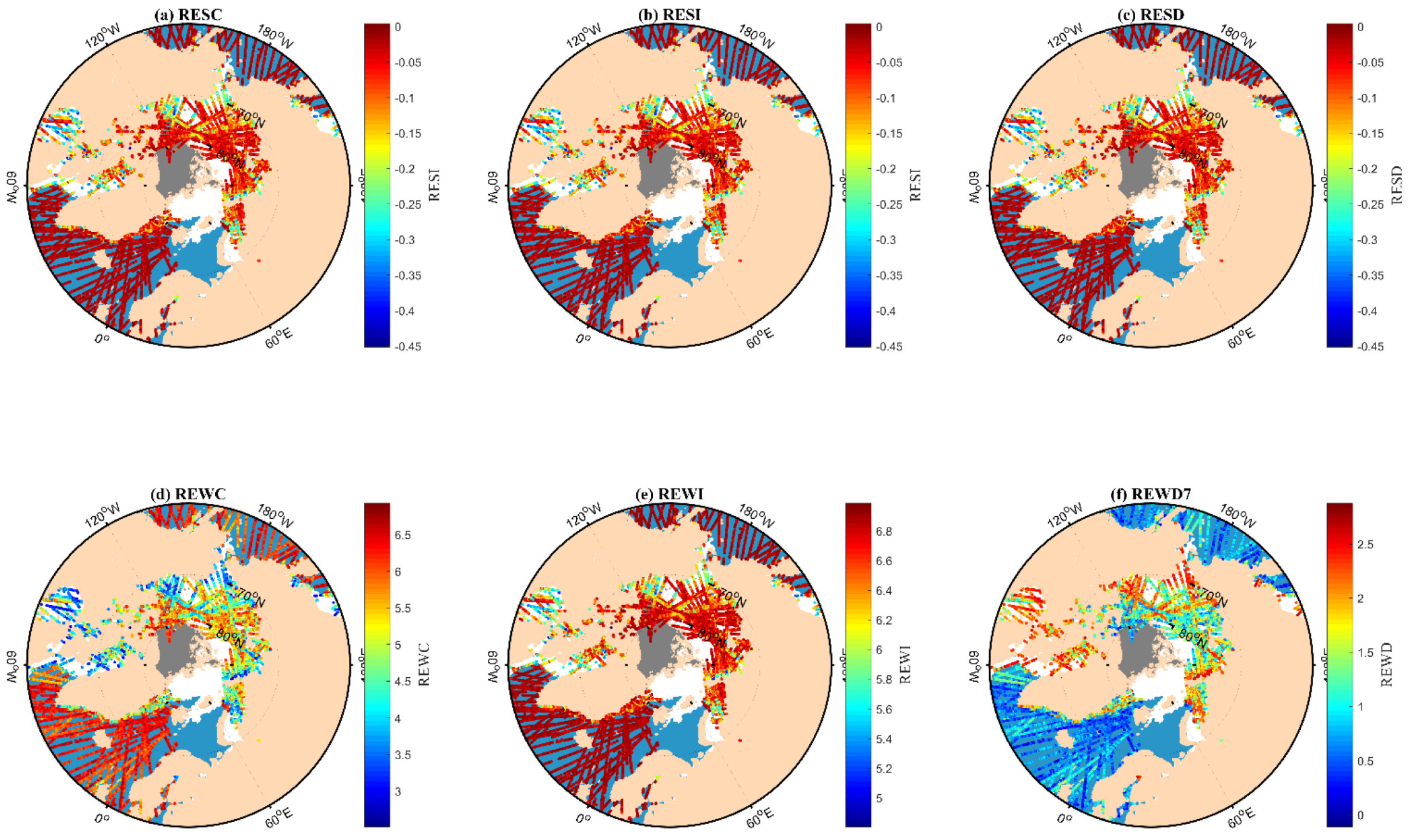
  • RESC (Right Edge Slope of CDW). The fitting slope of NCDW with 5 delay bins starting from the zero delay one is defined as RESC, which is depicted by the slope of the blue line in Figure 6a.
  • RESI (Right Edge Slope of IDW). The fitting slope of NIDW with 5 delay bins starting from the zero delay one is defined as RESI, which is depicted by the slope of the green line in Figure 6a.
  • RESD (Right Edge Slope of DDW). The fitting slope of DDW with 5 delay bins starting from the zero delay one is defined as RESD, which is depicted by the slope of the magenta line in Figure 6a.
  • REWC (Right Edge Waveform Summation of CDW). The summation of NCDW values (marked with blue diamond dots in Figure 6b) from the delay bins 0 to 6 is defined as REWC.
  • REWI (Right Edge Waveform Summation of IDW)}. The summation of NCDW values (marked with green cross dots in Figure 6b) from the delay bins 0 to 6 is defined as REWI.
  • REWD (Right Edge Waveform Summation of DDW)}. The summation of DDW values (marked with magenta circle dots in Figure 6b) from the delay bins 0 to 6 is defined as REWD.
The distribution of these six features versus the OSISAF SIT maps is illustrated in Figure 7.

3.2. Sea Ice Classification Method

Many previous studies indicate that RF and SVM show great potential in classifications [33,38,39,42], while they have not been used for classifying FYI and MYI using GNSS-R features. Thus, these two classifiers are used in this study to classify sea ice types.

3.2.1. Random Forest (RF)

The RF is one of the ensemble methods that have received increasing interest since they are more robust and accurate than single classifiers [52,53]. RF is composed of a set of classifiers where each classifier casts a vote for the allocation of the most frequent type to the input vectors. The principle of ensemble classifiers is based on the basic precondition that a variety of classifiers usually outperform an individual classifier. Some of the advantages of RF for remote sensing applications include (1) It has high efficiency on large datasets; (2) It can deal with a large number of input variables without variable deletion; (3) The variable importance can be estimated in the classification; (4) Relatively strong robustness to noise and outliers.
The design of a decision tree needs to choose an attribute selection measure and a pruning approach. The Gini index [54] is usually used to measure the impurity of training samples in RF. For a given training dataset T, the Gini index ( G i n d e x ) can be expressed as,
G i n d e x ( T ) = 1 i = 1 m p i 2 ,  
where m is the number of categories and p i is the proportion of samples T that belongs to class i. In the case of binary classification problems, the most appropriate characteristics at each node can be identified by the Gini index, given by:
G i n d e x ( T ) = 2 p ( 1 p ) .
The RF can also evaluate the relative importance of different features in the classification process. It is helpful to select the best features and know-how each feature influences the classification results [55,56].

3.2.2. Support Vector Machine (SVM)

SVM is a powerful machine learning algorithm based on statistical learning theory and has the purpose of determining the location of decision boundaries that produce the optimal separation of classes [57]. It is a supervised classification approach, which can deal with linear, nonlinear, high-dimensional samples and result in good generalization. SVM is primarily used for binary classification problems, in which the sample data can be expressed as,
( x 1 , y 1 ) , ( x 2 , y 1 ) , , ( x n , y n ) R n × Y , Y = ( 1 , 1 ) ,  
where x i represents the input samples that consist of features for classification, y i is the class label of x i For the linear classification, the SVM classifier satisfies the following rule,
y i ( w T x i + b ) 1 , 1 i n ,  
where w T x + b = 0 represents a hyperplane, with parameters w and b being the coefficient and bias, respectively. The maximum classification interval algorithm can be formulated as,
{ m i n ( 1 2 | | w | | 2 ) y i ( w T x i + b ) 1 .  
In order to obtain good predictions in nonlinear classification, the slack variables are introduced to express the soft margin optimal problem,
{ m i n ( 1 2 | | w | | 2 + C i = 1 n ξ i ) ξ i 0 , y i ( w T ϕ ( x i ) + b ) 1 ξ i , 1 i n ,  
where ξ i represents the ith slack variable, C is a penalty parameter. ϕ is a high-dimensional feature projection function related to the kernel function [58].

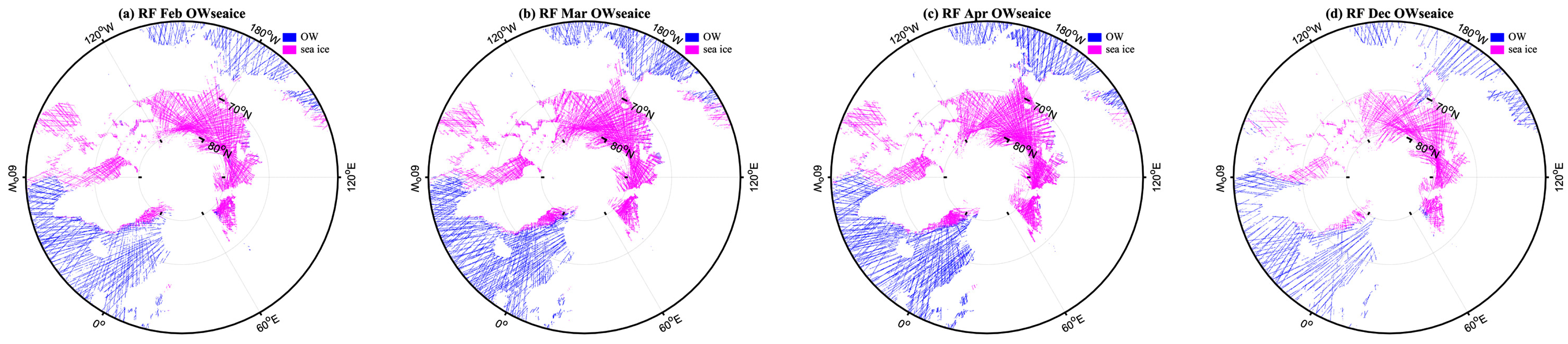
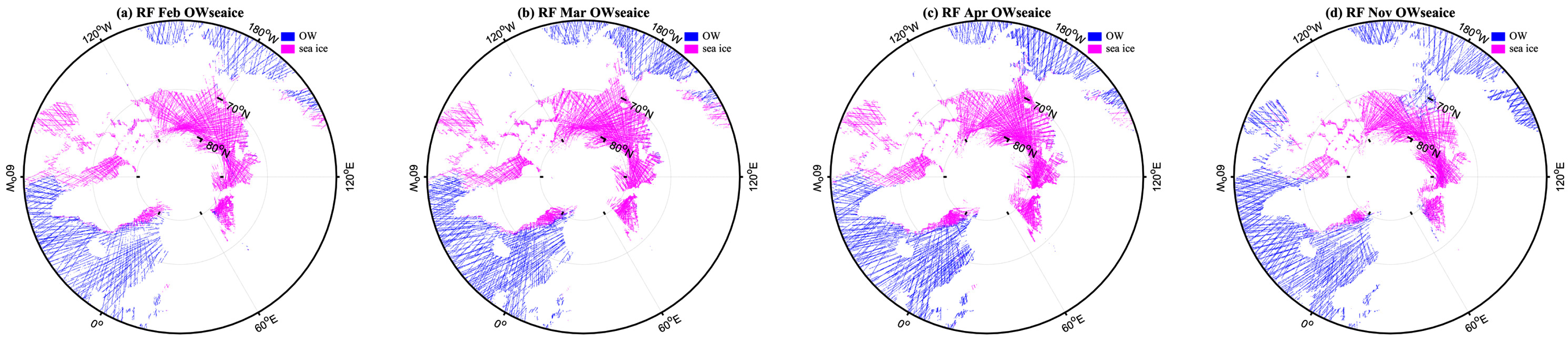
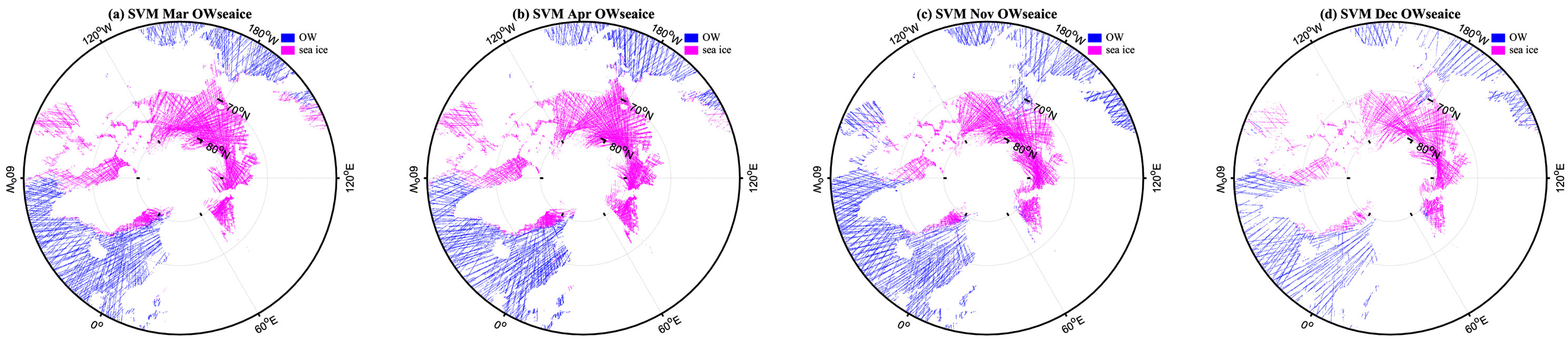
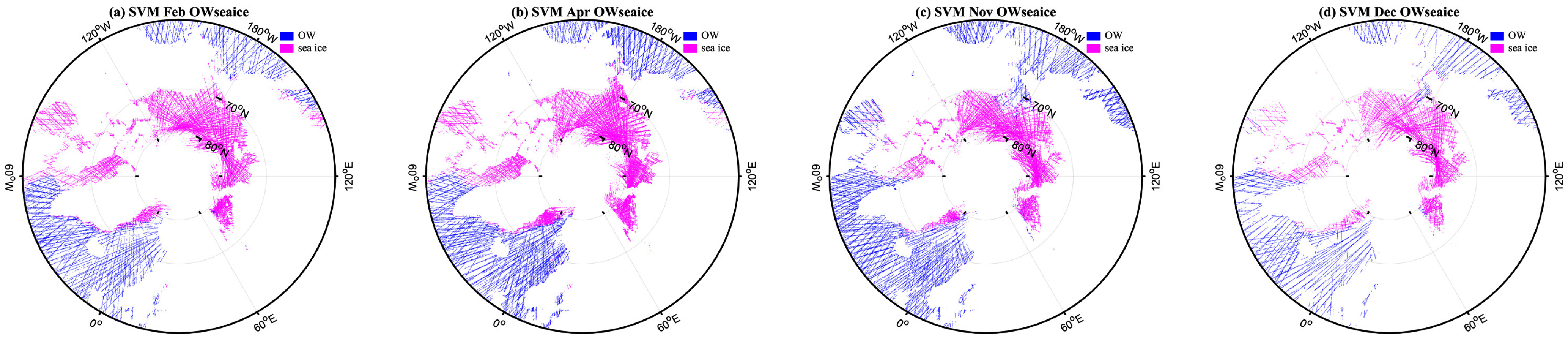
3.2.3. Sea Ice Classification Based on RF and SVM

In this study, the sea surface is divided into three categories, including OW, FYI, and MYI. As a powerful ML classifier, RF can deal with both binary and multi-classification problems. The strategy of one-against-one and one-against-all can be chosen to address the multi-classification problem. The RF classifier can be split into several binary classifiers using a one-against-all strategy (Anand et al., 1995) [59]. Although the standard RF algorithm can deal with multi-type problems, the one-against-all binarization to the RF can achieve better accuracy with smaller forest sizes than the standard RF [60]. In addition, the SVM is usually used for binary classification. Thus, the one-against-all binarization strategy is used in this study to classify OW, FYI, and MYI in two steps. In the first stage, the FYI and MYI are regarded as one category (sea ice), whereas the OW is regarded as another category. Then, the classification of sea ice types (FYI and MYI) will be carried out in the second stage using a similar method. The python software package from the Scikit-Learn is adopted in this study [61]. The process flow of sea ice classification is shown in Figure 8.
The sea ice classification method can be generally categorized into four parts:
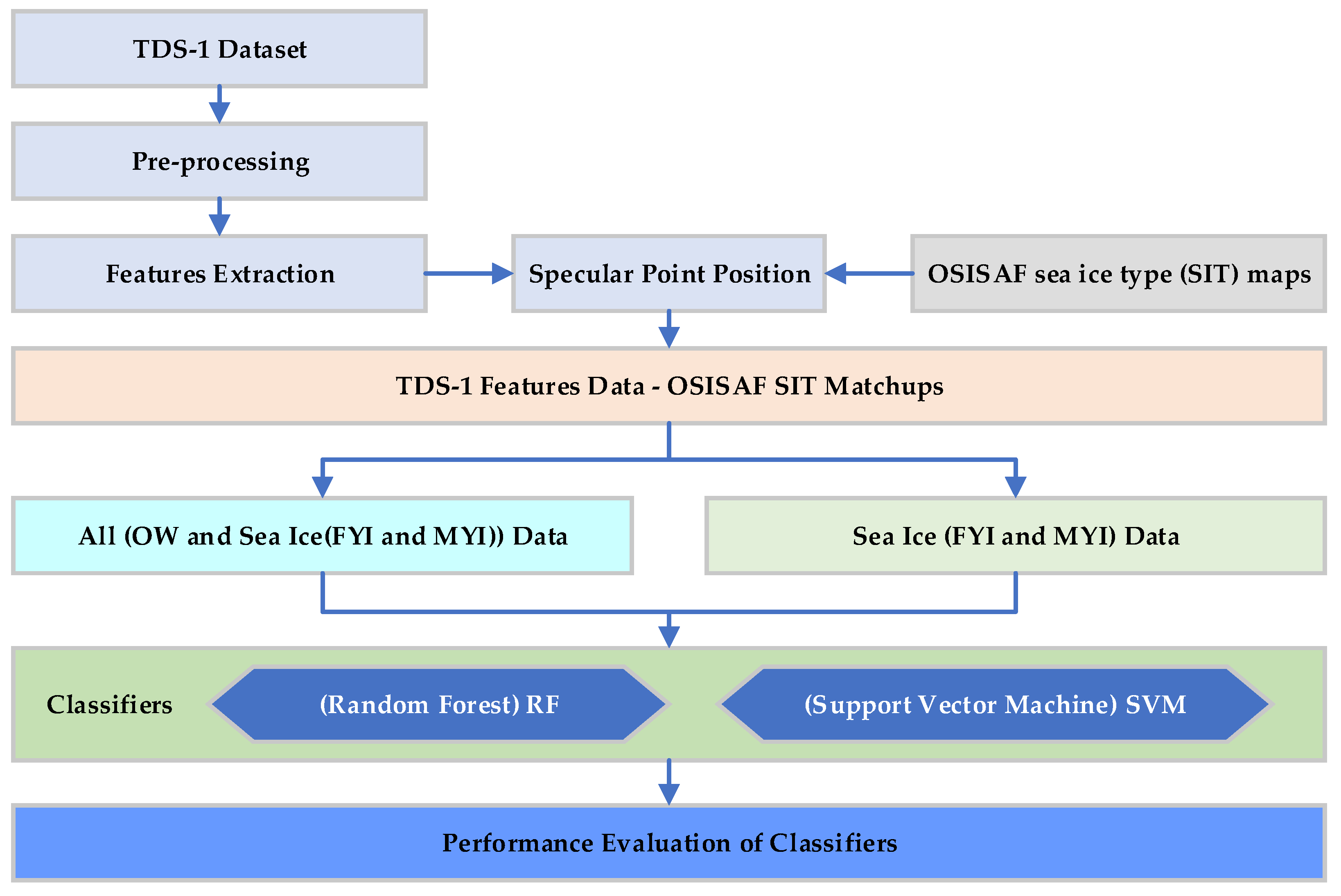
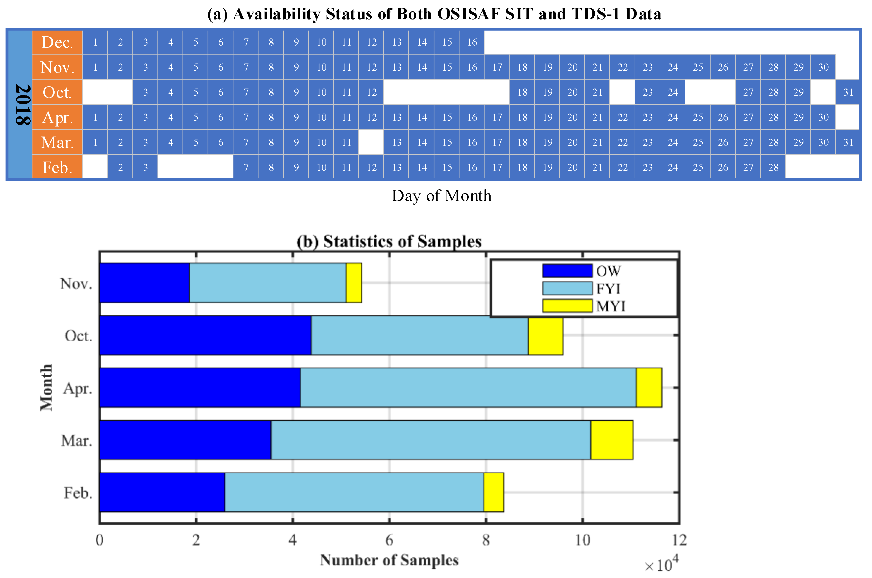
  • TDS-1 data preprocessing and features extraction. Firstly, the TDS-1 data with a latitude above 55°N and peak SNR above −3 dB is adopted to extract delay waveforms, which are further normalized to extract features. A total of eight features, namely SR, DDMA, RESC, RESI, RESD, REWC, REWI, and REWD, are extracted from the TDS-1 data. Then the TDS-1 features are matched with OSISAF SIT maps based on the data collection date and specular point position through a bilinear interpolation approach.
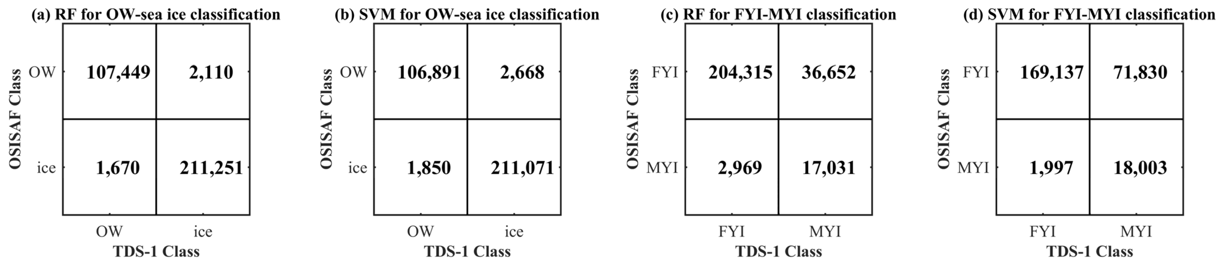
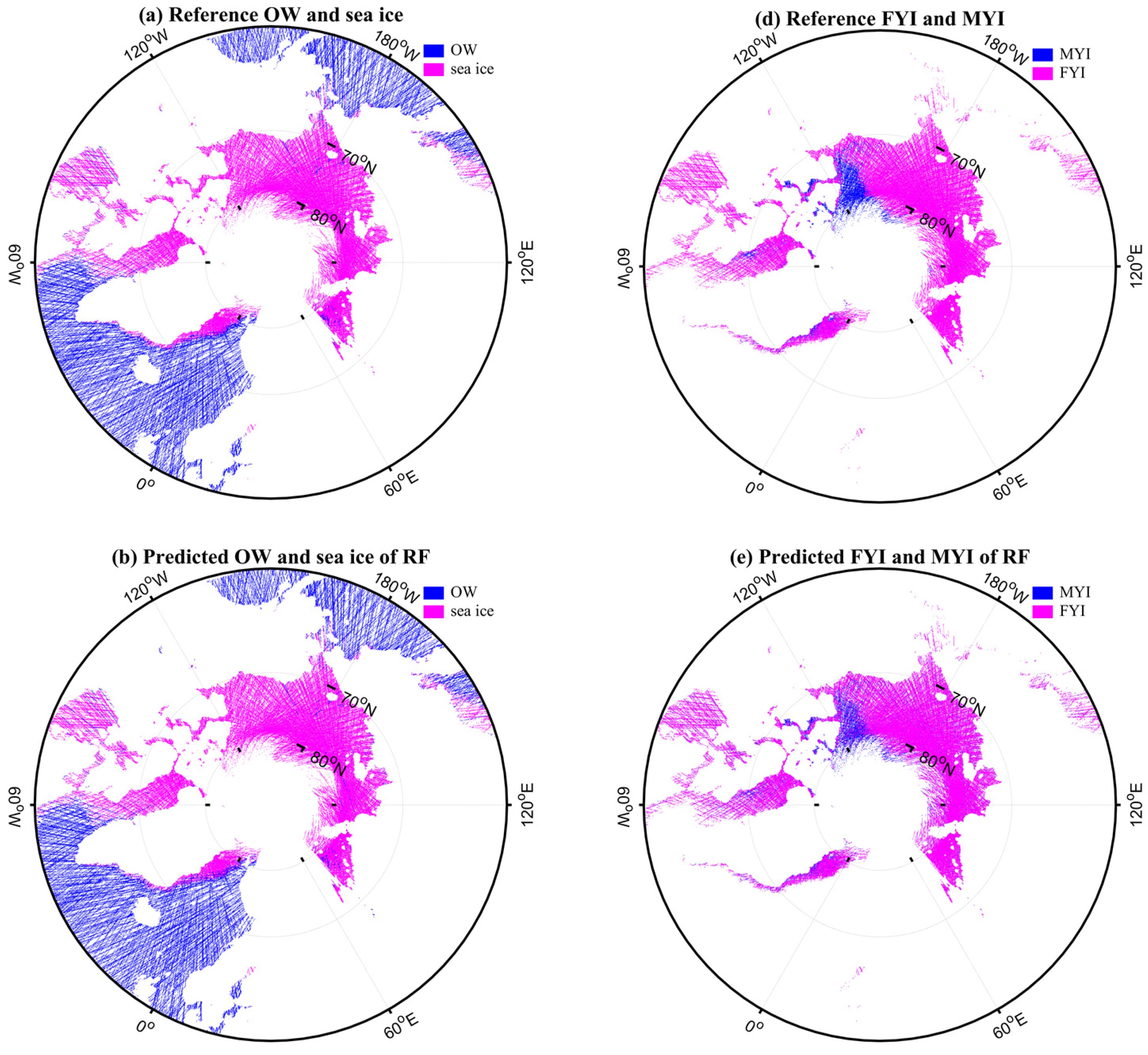
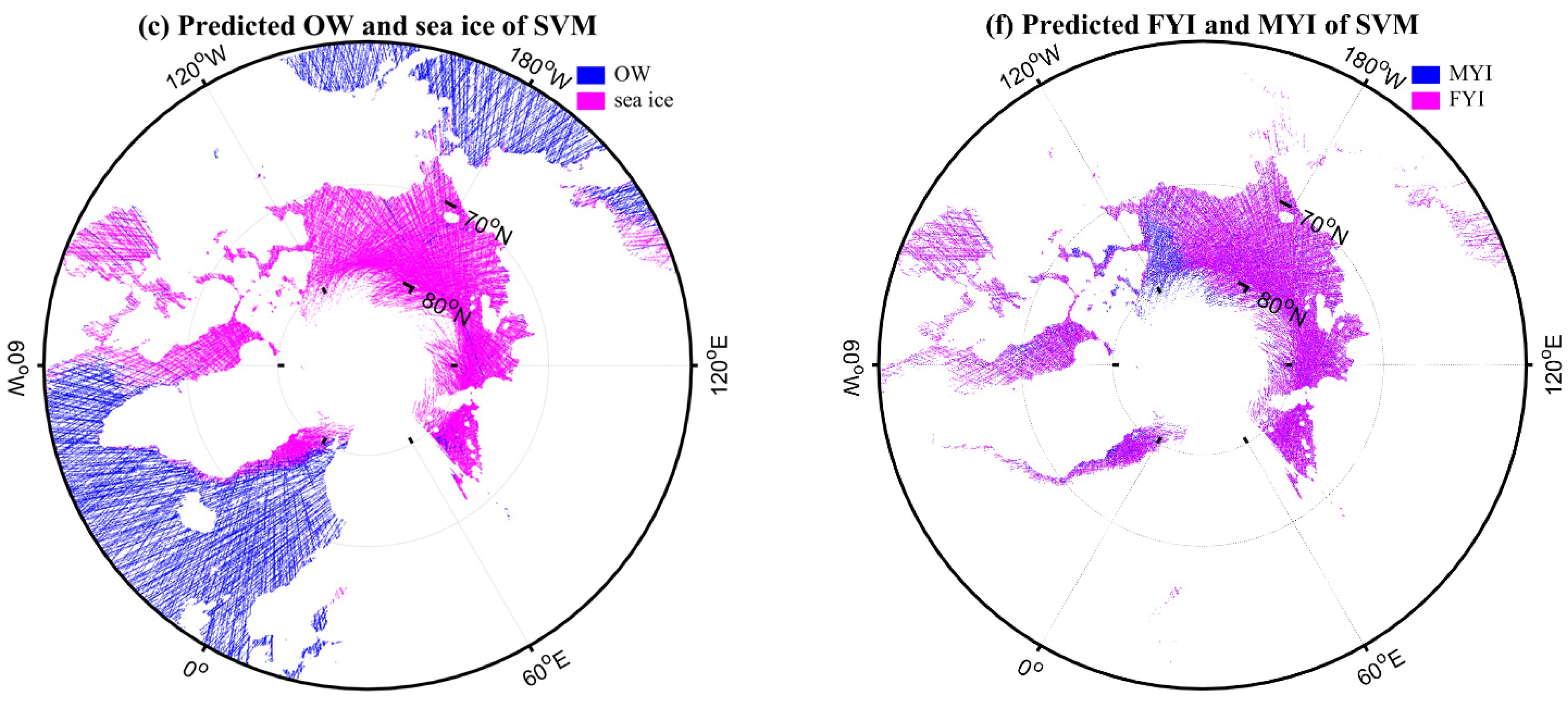
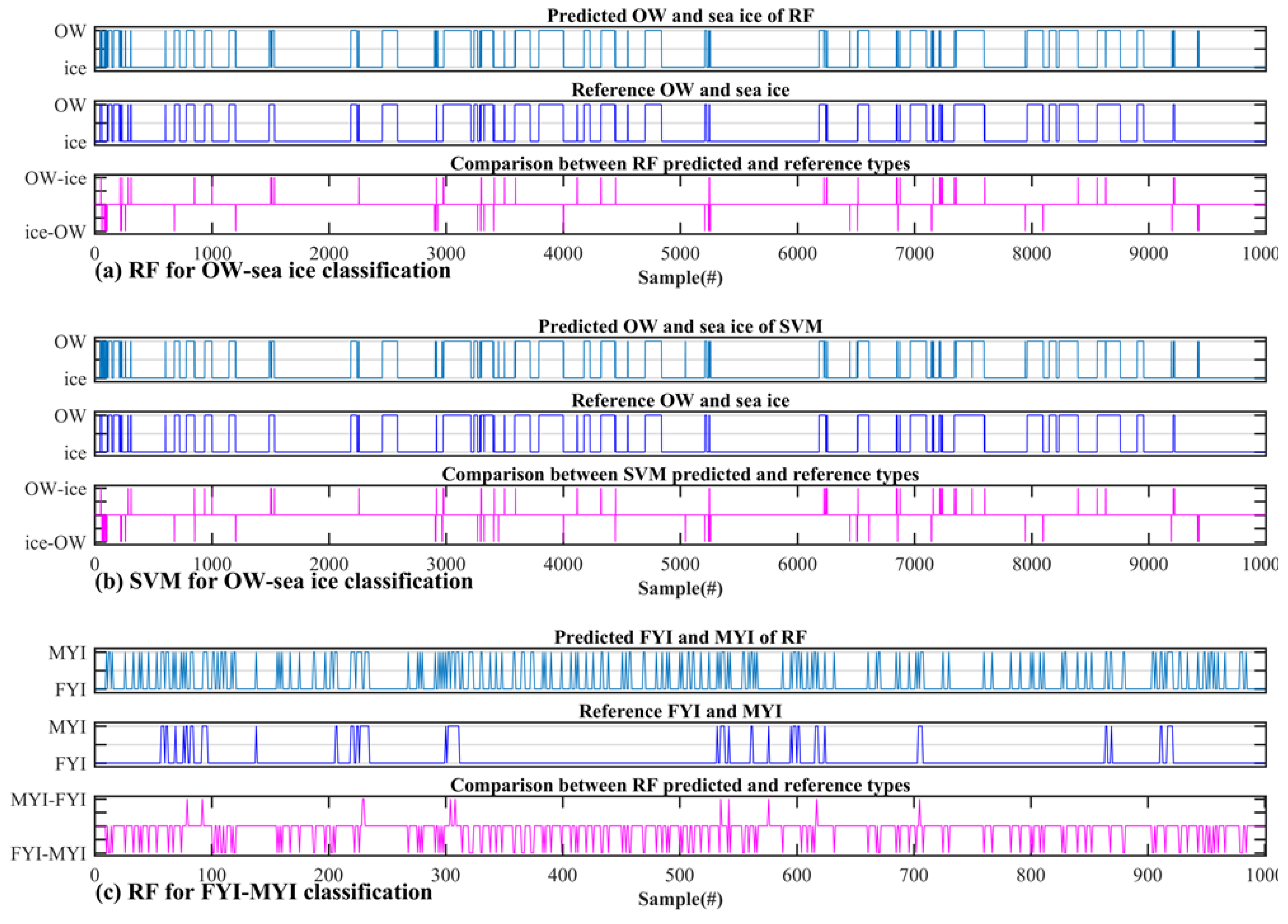
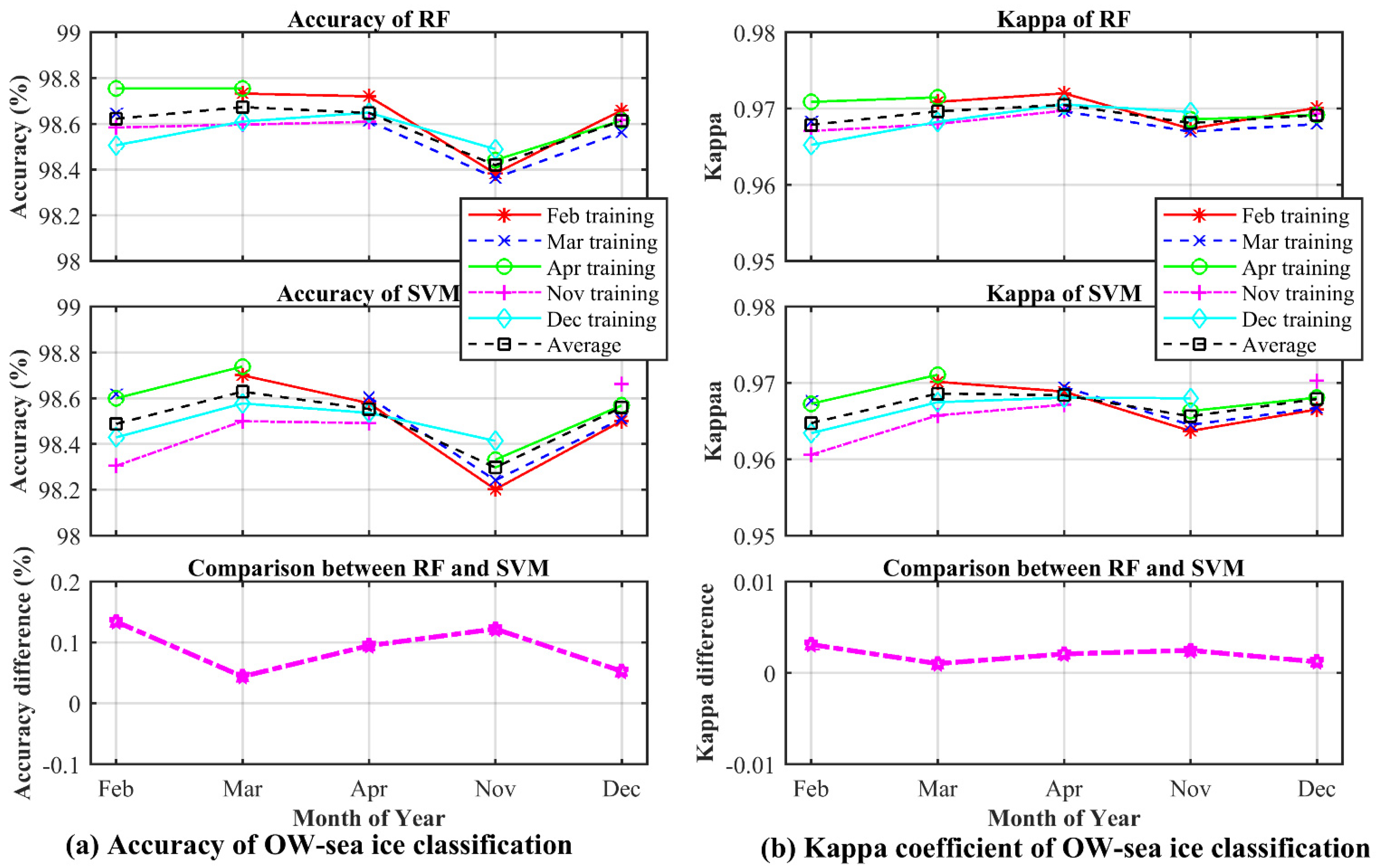
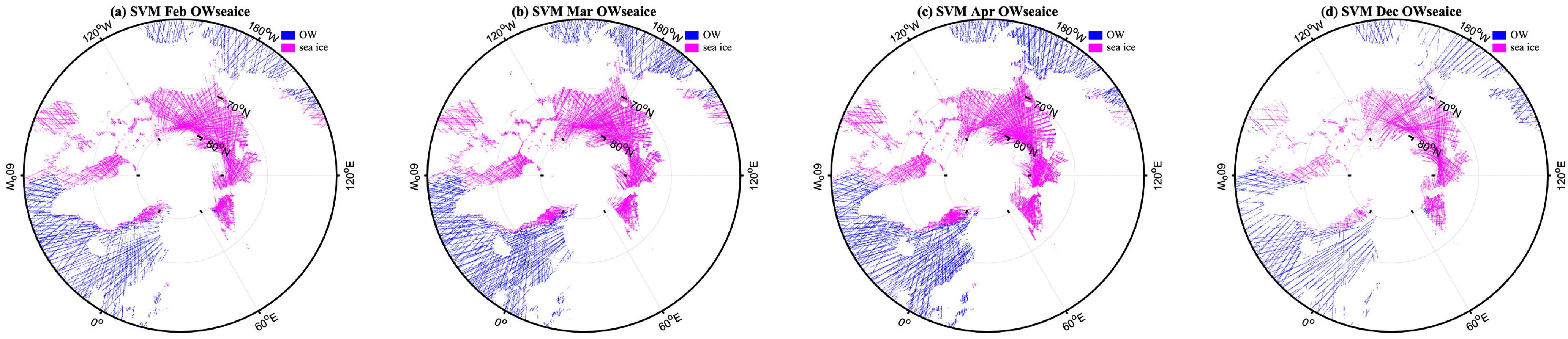
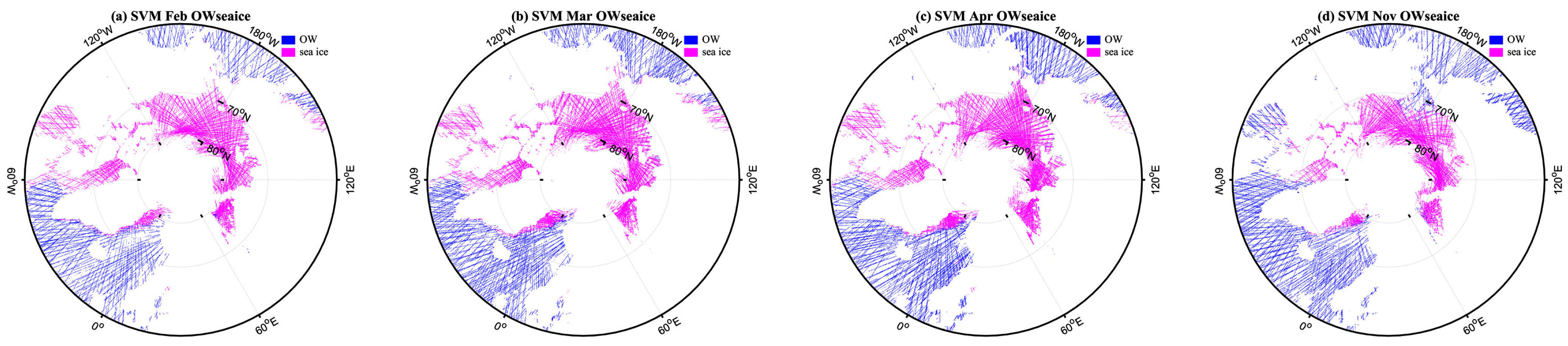
  • OW-sea ice classification. In this step, the FYI and MYI are regarded as one category (i.e., sea ice). 30% of samples are randomly selected as training set and the rest 70% of samples are used to test the OW-sea ice classification results.
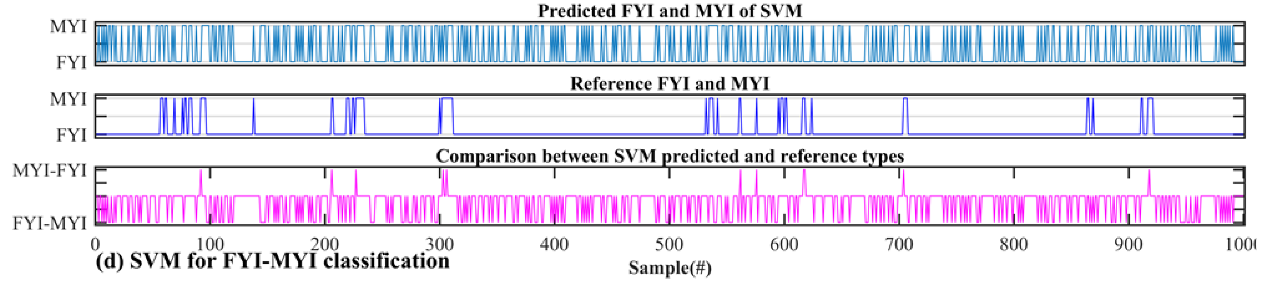
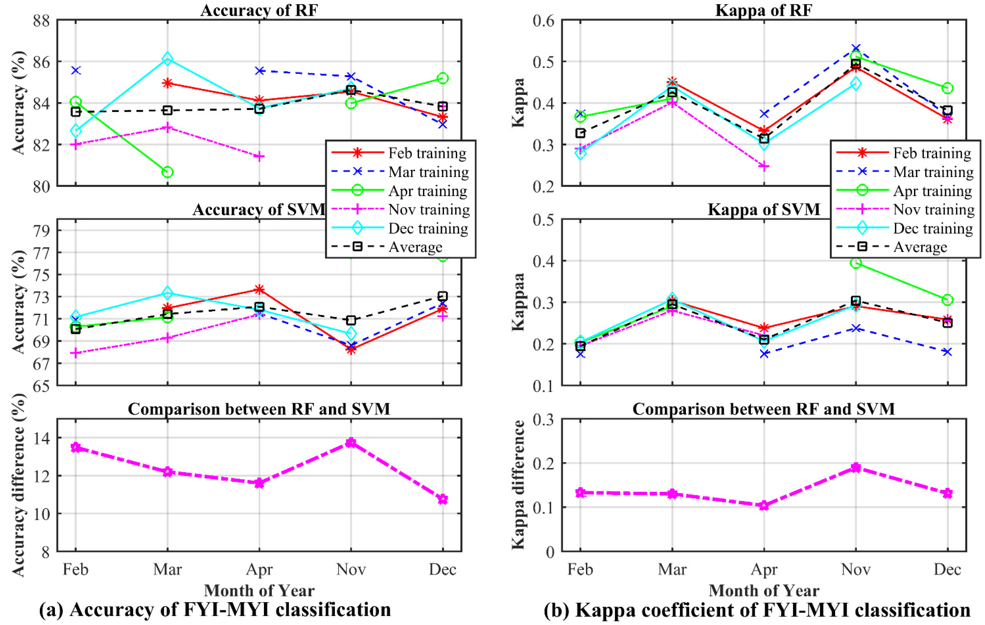
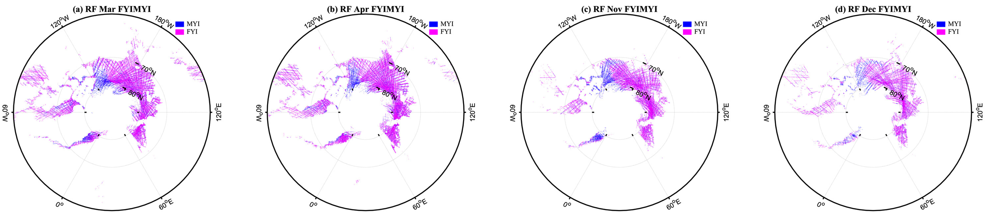
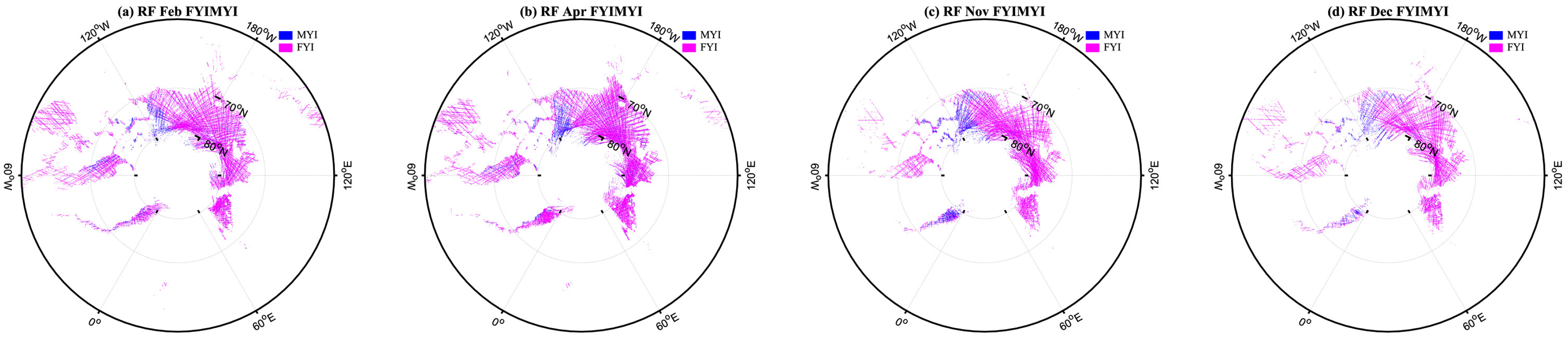
  • FYI-MYI classification. The sea ice datasets are applied in this step to classify FYI and MYI. As with the process of OW-sea ice classification, sea ice samples are randomly selected as training and test sets to classify FYI and MYI.
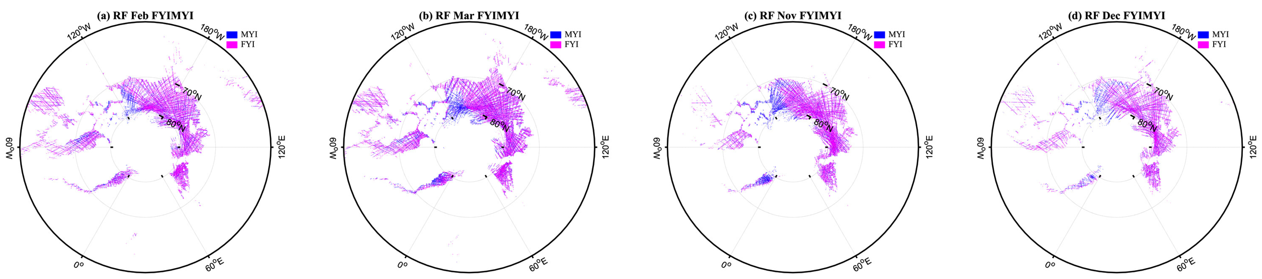
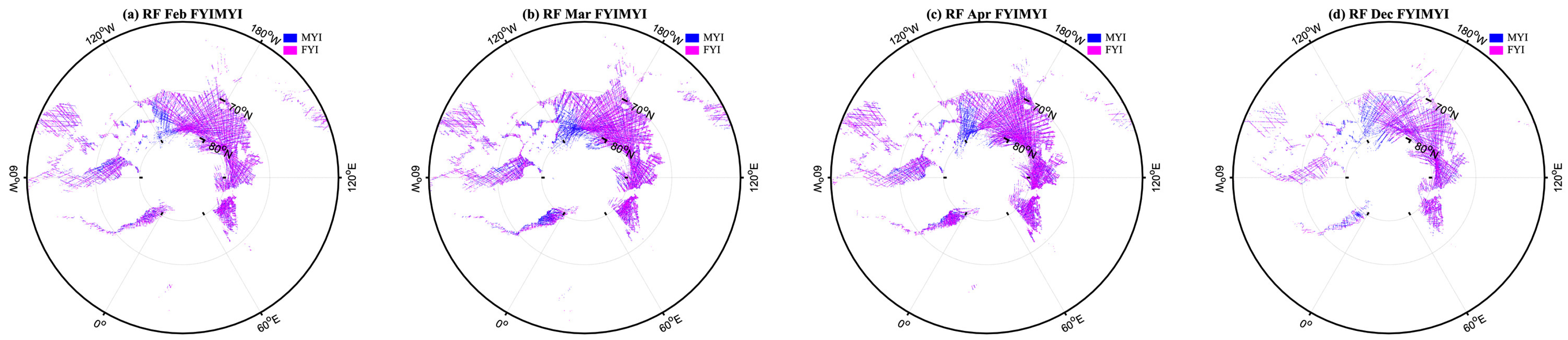
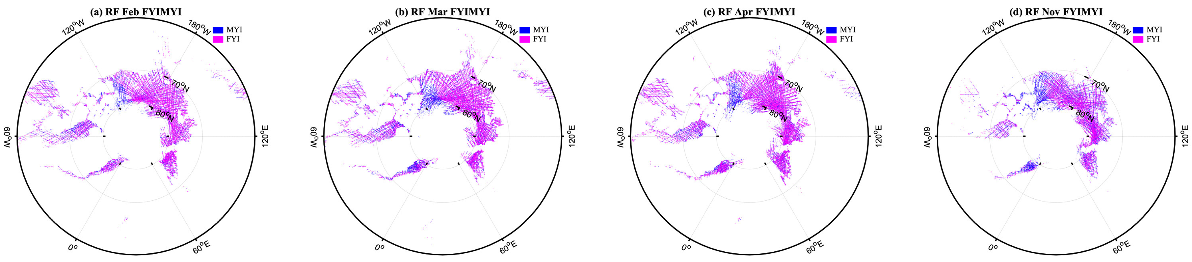
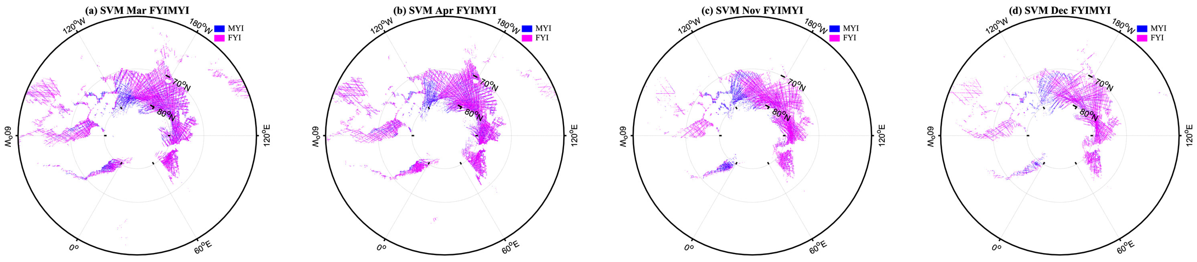
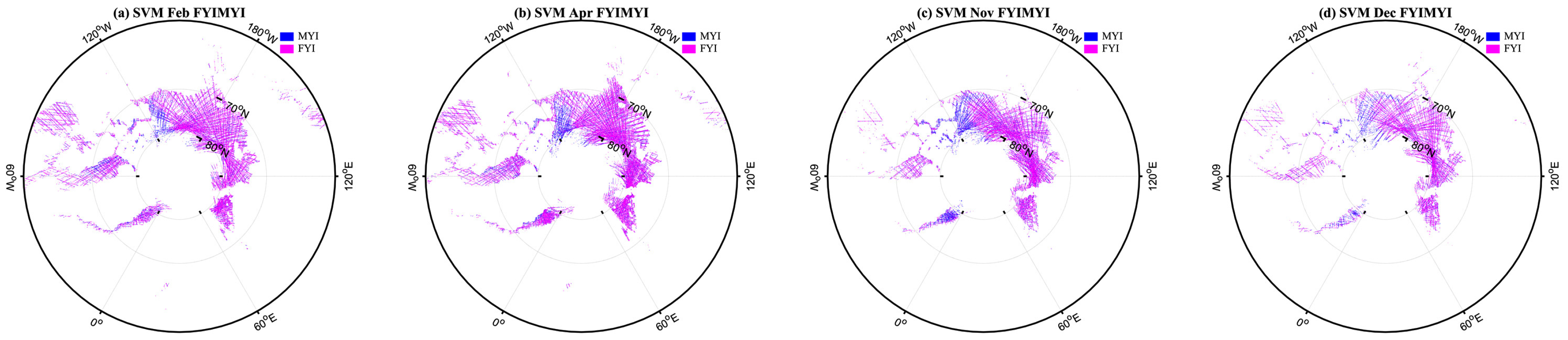
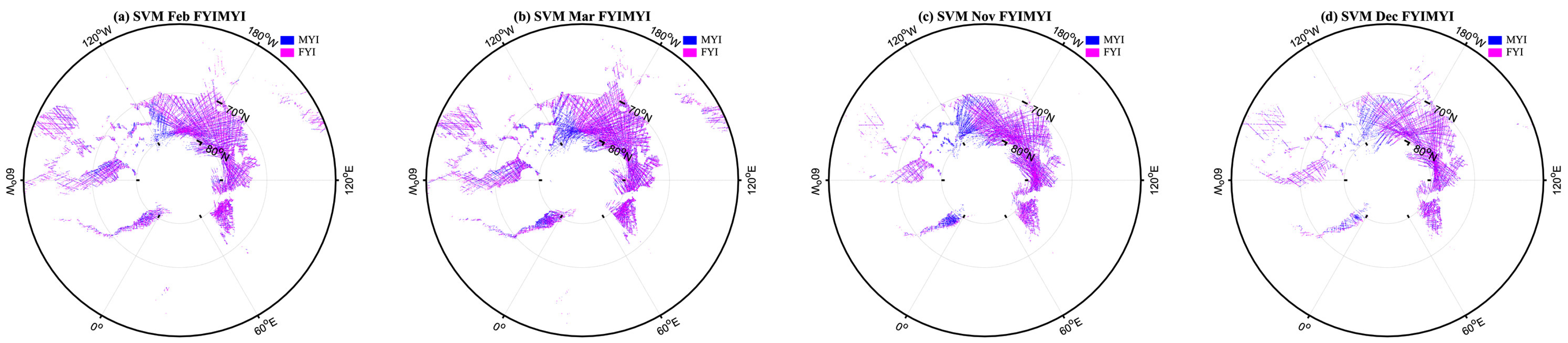
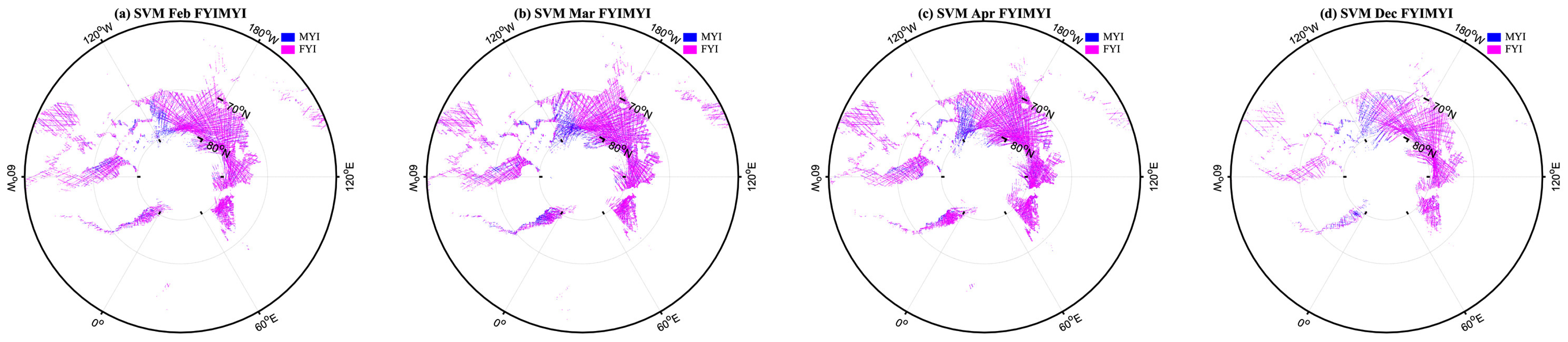
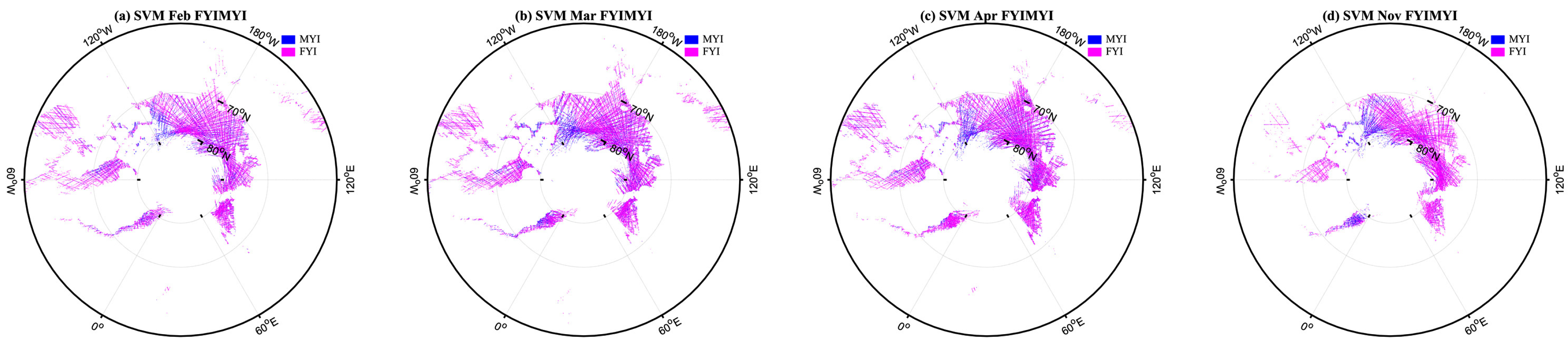
  • Performance evaluation of sea ice classification. The classification performance is firstly evaluated using the confusion matrix and some evaluation metrics, which are defined in Figure 9 and Table 3, respectively.
The row and column represent the actual and predicted types, respectively. As shown in Table 3, TP stands for the number of positive samples that are classified correctly. FN represents the number of positive samples that are classified into a negative type incorrectly. FP is the number of negative samples that are classified into a positive type incorrectly. TN is the number of negative samples that are classified correctly. The evaluation metrics that are used to evaluate the classification performance are defined in Table 3. Accuracy represents the ratio of the correct classification number in all the samples. Precision depicts the precision of predicted results that positive samples are classified correctly. Recall means the completeness of the samples that are classified correctly in all positive samples. F-value is the harmonic mean of classification performance for positive samples, where β is usually set as 1. Then the F-value is the F1 score, which is the weighted average of Precision and Recall. Therefore, this score takes both false positives and false negatives into account. G-mean can be used to evaluate the overall classification performance. G-mean measures the balance between classification performances on both the majority and minority classes. In addition, the kappa coefficient is also used to measure inter-rater reliability for classifiers. The kappa coefficient measures the agreement between two raters who each classify N items into C mutually exclusive categories.

4. Results

Although the OSISAF SIT products are provided continuously, there is a lack of MYI information from May to October most of the time in the OSISAF SIT products. In addition, the TDS-1 data is very sparse from 2015 to 2017 as the GNSS-R receiver was working only two days in an eight-day cycle. Therefore, the TDS-1 datasets collected in 2018 are selected according to the availability of MYI information of OSISAF SIT products. Figure 10a presents the data availability status of both OSISAF SIT products and TDS-1 data that are used in this study. The number of OW, FYI, and MYI samples every month are shown in Figure 10b. According to the statistics, a total number of 460,685 samples, including 165,434 OW samples, 266,680 FYI samples, and 28,571 MYI samples, are used in this study.
As illustrated in Section 3, the sea ice classification is implemented using a two-step method. The first step aims to discriminate OW from sea ice using the RF and SVM classifiers. During the RF model training, the number of trees is set to different values ranging from 10 to 200, in order to find the best classifier. The number of estimators is finally set as 70 in this study. After identifying the OW, the sea ice samples are employed to classify FYI and MYI in the second step using the RF classifier. It is worth noting that the number of FYI samples is about nine times that of MYI samples. When randomly selecting samples from the whole FYI and MYI dataset as the training set, only a small amount of MYI samples are selected out. The proportion gap between FYI and MYI samples in the training set is too large and the training model may not grasp the features of MYI. Therefore, 30% of MYI samples are randomly selected as training set and the number of FYI samples is controlled to be three times that of MYI.
The confusion matrix of RF and SVM classifiers are presented in Figure 11, which presents the classification results of each class. Table 4 presents the evaluation metrics which are computed according to equations listed in Table 3.
Table 4 demonstrates the evaluation metrics through validating with the OSISAF SIT maps using the test dataset. As shown in Figure 11a,b, a total of 322,480 samples, which include 109,559 OW and 212,921 sea ice samples, are applied for testing. The overall accuracy of RF and SVM classifiers for OW-sea ice classification is 98.83% and 98.60% respectively, which are comparable to the results in previous studies [15,38,40]. Similarly, the FYI-MYI classification results are evaluated using 20,000 FYI samples and 240,967 MYI samples (Figure 11c,d), which results in an overall accuracy of 84.82% for RF, whereas 71.71% for SVM. The performance of RF and SVM for OW-sea ice classification is comparable, whereas RF outperforms SVM significantly in the FYI-MYI classification. The overall space distribution of classification results is shown in Figure 12, which depicts the distribution of predicted and reference types. For illustration purposes, parts of classifications are shown in Figure 13, which demonstrates the predicted, reference, and their comparison results. Firstly, sea ice and OW are labeled as −1 and 1, respectively, in the OW-sea ice classification, whereas FYI and MYI are labeled as −1 and 1, respectively, in the FYI-MYI classification. The comparison results between predicted and reference types are computed as follows,
D i f f = R e f     P r e ,  
where Ref represents the value of reference types, Pre is the value of predicted types, Diff is the comparison results. In the OW-sea ice classification, −2 represents the sea ice is misclassified as OW (ice-OW), 2 represents the OW is misclassified as sea ice (OW-ice), and 0 means the predicted and reference type is consistent. In the FYI-MYI classification, −2 represents the FYI is misidentified as MYI (FYI-MYI), 2 represents the MYI is misidentified as FYI (MYI-FYI), and 0 means the predicted and reference type is consistent.
As shown in Figure 12b,c, most OW and sea ice misclassifications of RF and SVM classifiers appear similarly at the points of OW-sea ice transitions. This can also be seen in Figure 13a,b. The confusion matrix in Figure 11c,d presents that the number of FYI misclassifications is much larger than that of MYI misclassifications. This may be due to the large gap in the number of FYI and MYI samples. The overall accuracy is affected less by the MYI misclassifications since the number of FYI samples is more than 10 times that of MYI samples. As shown in Figure 12e,f, both RF and SVM classifiers have lots of misclassifications, which are widely distributed. In general, the number of misclassifications of SVM is more than that of RF, which can also be seen in Figure 13c,d. In addition, the kappa coefficient of OW-sea ice classification is 0.97 both for RF and SVM, whereas that of FYI-MYI is only 0.39 and 0.23 respectively for RF and SVM. In addition, although SVM can achieve comparable accuracy as RF in OW-sea ice classification, the time consumption of SVM is about nine times that of RF for the same test dataset.

5. Discussion

In order to analyze the influence of sea ice growth and melt on sea ice classification and the robustness of the sea ice classification method, another experiment is implemented. Each month of data is used as a training set individually, and the remaining four months of data are used as a test set. The strategy is similar to k-fold cross-validation [62] usually applied in ML. However, the k-fold cross-validation is to split the dataset into k parts randomly, which would eliminate the seasonal effects. Firstly, the data in February are used as the training set, and the data in March, April, November, and December are used as the testing set in turn. Hereafter, the data in Mar, April, November, and December are used as training set successively. The space distribution of classification results is presented in Appendix A (Figure A1, Figure A2, Figure A3, Figure A4, Figure A5, Figure A6, Figure A7, Figure A8, Figure A9 and Figure A10) and Appendix B (Figure A11, Figure A12, Figure A13, Figure A14, Figure A15, Figure A16, Figure A17, Figure A18, Figure A19 and Figure A20). The accuracy and kappa coefficients of OW-sea ice and FYI-MYI classification are shown in Figure 14 and Figure 15, which indicate that the overall accuracy of OW-sea ice changes less than that of FYI-MYI classification. This may be caused by the change of samples distribution as the proportion of OW and sea ice is relatively stable, while that of FYI and MYI changes more easily with ice growth and melt.
As shown in Figure 14, the accuracy of OW-sea ice classification changes slightly from February to April and then drops from April to November, followed by a larger increase from November to December. The accuracy in November reaches the lowest point among all tested months. Figure 15 demonstrates that the general changing trend of accuracy for FYI-MYI classification is similar to that for OW-sea ice classification. This can be explained in combination with the sea ice extent trend in 2018, shown in Figure 16. As shown in Figure 16a, the sea ice extent reached the maximum and minimum on 14 March 2018 and 21 September 2018, respectively. The sea ice extent increases firstly to the peak sea ice extent and then decreases slightly from March to April, while it increases continuously from November to December. Moreover, among five months of use, the ice extent in November is the smallest (Figure 16b). The increase and decrease of sea ice extent can be regarded as ice growth and melt process, respectively. The ice extent during February to April changes less than that during November to December since November is a period of the early stage of winter. The sea ice extent during February to April is relatively stable. From February to March, the FYI grows and the presence of ocean water in FYI becomes less, which results in less misclassification for FYI. During the melting process from March to April, the surface of FYI can be more easily affected by ocean winds due to the decrease of sea ice concentration of FYI. This may lead to more misclassification of FYI to MYI. The overall accuracy for OW-sea ice and FYI-MYI classification in November is the smallest. The explanation is that the sea ice extent is relatively low in November when newly added sea ice is mostly surrounded by ocean water, which leads to more misclassifications. With the ice growth from November to December, the successful classification rate increases relatively obviously, which is consistent with the sea ice extent trend shown in Figure 16.

6. Conclusions

This study investigates the RF and SVM-based classifiers for Arctic Sea ice classification using the one-against-all binarization, which converts a multi-classification into several binary classification problems. Thus, the classification is implemented in a two-step way. The first step aims to discriminate OW from sea ice (FYI and MYI), which is further classified in the second step. The selected data periods include February to April and November to December in 2018, during which the information of different surface types (OW, FYI, and MYI) is available and can be used for comparison. Through validating against OSISAF SIT maps, the overall accuracy of the RF and SVM for OW-sea ice classification is up to 98.83% and 98.60%, which is comparable to results from some previous studies using TDS-1 data [15,30,38,39,40]. Hereafter, the FYI-MYI classifier is modeled in the second using the samples of sea ice that include FYI and MYI. The overall accuracy of RF and SVM for classifying FYI and MYI is 84.82% and 71.71%, respectively, which are lower than those of the OW-sea ice classifier. Moreover, the influence of ice growth and melt for sea ice classification is evaluated through a cross-validating strategy, which applies each month of data as the training set and the remaining four months of data as the test set. To the best of the author’s knowledge, the RF and SVM are firstly used for classifying FYI and MYI using the spaceborne GNSS-R data. The results indicate that RF and SVM-based GNSS-R have great potential in sea ice classification. This study demonstrates that the great potential of GNSS-R for classifying sea ice types, which can be an effective and complementary approach for remotely sensing sea ice. In future studies, more GNSS-R features, ML algorithms, and environmental effects (such as ocean wind) should be investigated to improve the accuracy of classifying FYI and MYI.

Author Contributions

Conceptualization, Y.Z. and T.T.; methodology, Y.Z.; software, Y.Z., J.L. and T.T.; validation, Y.Z. and T.T.; formal analysis, Y.Z.; investigation, Y.Z.; resources, Y.Z.; data curation, Y.Z.; writing—original draft preparation, Y.Z.; writing—review and editing, Y.Z., K.Y., L.W., X.Q., S.L., J.W. and M.S.; visualization, Y.Z.; supervision, T.T. and K.Y.; project administration, Y.Z.; funding acquisition, Y.Z. All authors have read and agreed to the published version of the manuscript.

Funding

This research was funded in part by Natural Science Foundation of Anhui Province, China, grant number 2108085QD176, by National Natural Science Foundation of China, grant number 42104019, 42171141, 42174022, by the open research fund of State Key Laboratory of Information Engineering in Surveying, Mapping and Remote sensing, Wuhan University, grant number 20P04, by the Fundamental Research Funds for the Central Universities of China, grant number JZ2020HGTA0087, by the Key Laboratory of Geospace Environment and Geodesy, Ministry of Education, Wuhan University, grant number 19-01-03, by the Key Laboratory for Digital Land and Resources of Jiangxi Province, East China University of Technology, grant number DLLJ202001.

Institutional Review Board Statement

Not applicable.

Informed Consent Statement

Not applicable.

Data Availability Statement

The spaceborne GNSS-R data from TDS-1 mission is available at www.merrbys.co.uk. The sea ice type (SIT) and sea ice concentration (SIC) products are downloaded from the EUMETSAT OSISAF data portal on 18 February 2021 (http://osisaf.met.no/, accessed on 11 September 2021).

Acknowledgments

The authors would like to thank the TechDemoSat-1 team at Surrey Satellite Technology Ltd. (SSTL) for providing the spaceborne GNSS-R data. Our gratitude also to Ocean and Sea Ice Satellite Application Facility for the sea ice edge product used in comparisons.

Conflicts of Interest

The authors declare no conflict of interest.

Abbreviations

The following abbreviations are used in this manuscript:
CDWCentral Delay Waveform
CYGNSSCyclone Global Navigation Satellite System
DDMDelay-Doppler Map
DDMADelay-Doppler Map Average
DDWDifferential Delay Waveform
EIRPEffective Isotropic Radiated Power
EUMETSATEuropean Organization for the Exploitation of Meteorological Satellites
FYIFirst-Year Ice
GNSSGlobal Navigation Satellite System
GNSS-RGlobal Navigation Satellite System Reflectometry
IDWIntegrated Delay Waveform
MLMachine Learning
MYIMulti-Year Ice
NCDWNormalized Central Delay Waveform
NIDWNormalized Integrated Delay Waveform
NSIDCNational Snow and Ice Data Center
OSI SAFOcean and Sea Ice Satellite Application Facility
OWOpen Water
RESCRight Edge Slope of CDW
RESDRight Edge Slope of DDW
RESIRight Edge Slope of IDW
REWCRight Edge Waveform Summation of CDW
REWDRight Edge Waveform Summation of DDW
REWIRight Edge Waveform Summation of IDW
RFRandom Forest
SICSea Ice Concentration
SITSea Ice Type
SNRSignal-to-Noise Ratio
SPSpecular Point
SSMISSpecial Sensor Microwave Imager Sounder
SVMSupport Vector Machine
TDS-1TechDemoSat-1

Appendix A

Appendix A presents the results of RF and SVM for OW-sea ice classification using each month of data as the training set in turn. The RF classifier results are shown in Figure A1, Figure A2, Figure A3, Figure A4 and Figure A5, and the SVM classifier results are presented in Figure A6, Figure A7, Figure A8, Figure A9 and Figure A10. In each figure title, the RF and SVM represent method, then followed by the test data of month, such February, March, April, November, December, and OWseaice represents OW-sea ice classification.
Figure A1. RF for OW-sea ice classification using the data in February as the training set. The data in (a) March, (b) April, (c) November, and (d) December are used as the test set in turn.
Remotesensing 13 04577 g0a1
Figure A2. RF for OW-sea ice classification using the data in March as the training set. The data in (a) February, (b) April, (c) November, and (d) December are used as the test set in turn.
Remotesensing 13 04577 g0a2
Figure A3. RF for OW-sea ice classification using the data in April as the training set. The data in (a) February, (b) March, (c) November, and (d) December are used as the test set in turn.
Remotesensing 13 04577 g0a3
Figure A4. RF for OW-sea ice classification using the data in November as the training set. The data in (a) February, (b) March, (c) April, and (d) December are used as the test set in turn.
Remotesensing 13 04577 g0a4
Figure A5. RF for OW-sea ice classification using the data in December as the training set. The data in (a) February, (b) March, (c) April, and (d) November are used as the test set in turn.
Remotesensing 13 04577 g0a5
Figure A6. SVM for OW-sea ice classification using the data in February as the training set. The data in (a) March, (b) April, (c) November, and (d) December are used as the test set in turn.
Remotesensing 13 04577 g0a6
Figure A7. SVM for OW-sea ice classification using the data in March as the training set. The data in (a) February, (b) April, (c) November, and (d) December are used as the test set in turn.
Remotesensing 13 04577 g0a7
Figure A8. SVM for OW-sea ice classification using the data in April as the training set. The data in (a) February, (b) March, (c) November, and (d) December are used as the test set in turn.
Remotesensing 13 04577 g0a8
Figure A9. SVM for OW-sea ice classification using the data in November as the training set. The data in (a) February, (b) March, (c) April, and (d) December are used as the test set in turn.
Remotesensing 13 04577 g0a9
Figure A10. SVM for OW-sea ice classification using the data in December as the training set. The data in (a) February, (b) March, (c) April, and (d) November are used as the test set in turn.
Remotesensing 13 04577 g0a10

Appendix B

Appendix B presents the results of RF and SVM for FYI-MYI classification using each month of data as the training set in turn. The RF classifier results are shown in Figure A11, Figure A12, Figure A13, Figure A14 and Figure A15, and the SVM classifier results are presented in Figure A16, Figure A17, Figure A18, Figure A19 and Figure A20. In each figure title, the RF and SVM represent method, then followed by the test data of month, such Feb, Mar, Apr, Nov, Dec, and FYIMYI represents FYI-MYI classification.
Figure A11. RF for FYI-MYI classification using the data in February as the training set. The data in (a) March, (b) April, (c) November, and (d) December are used as the test set in turn.
Remotesensing 13 04577 g0a11
Figure A12. RF for FYI-MYI classification using the data in March as the training set. The data in (a) February, (b) April, (c) November, and (d) December are used as the test set in turn.
Remotesensing 13 04577 g0a12
Figure A13. RF for FYI-MYI classification using the data in April as the training set. The data in (a) February, (b) March, (c) November, and (d) December are used as the test set in turn.
Remotesensing 13 04577 g0a13
Figure A14. RF for FYI-MYI classification using the data in November as the training set. The data in (a) February, (b) March, (c) April, and (d) December are used as the test set in turn.
Remotesensing 13 04577 g0a14
Figure A15. RF for FYI-MYI classification using the data in December as the training set. The data in (a) February, (b) March, (c) April, and (d) November are used as the test set in turn.
Remotesensing 13 04577 g0a15
Figure A16. SVM for FYI-MYI classification using the data in February as the training set. The data in (a) March, (b) April, (c) November, and (d) December are used as the test set in turn.
Remotesensing 13 04577 g0a16
Figure A17. SVM for FYI-MYI classification using the data in March as the training set. The data in (a) February, (b) April, (c) November, and (d) December are used as the test set in turn.
Remotesensing 13 04577 g0a17
Figure A18. SVM for FYI-MYI classification using the data in April as the training set. The data in (a) February, (b) March, (c) November, and (d) December are used as the test set in turn.
Remotesensing 13 04577 g0a18
Figure A19. SVM for FYI-MYI classification using the data in November as the training set. The data in (a) February, (b) March, (c) April, and (d) December are used as the test set in turn.
Remotesensing 13 04577 g0a19
Figure A20. SVM for FYI-MYI classification using the data in December as the training set. The data in (a) February, (b) March, (c) April, and (d) November are used as the test set in turn.
Remotesensing 13 04577 g0a20

References

  1. Screen, J.A.; Simmonds, I. The central role of diminishing sea ice in recent Arctic temperature amplification. Nature 2010, 464, 1334–1337. [Google Scholar] [CrossRef] [Green Version]
  2. Park, J.-W.; Korosov, A.A.; Babiker, M.; Won, J.-S.; Hansen, M.W.; Kim, H.-C. Classification of sea ice types in sentinel-1 SAR images. Cryosphere Discuss 2019, 2019, 1–23. [Google Scholar]
  3. Dabboor, M.; Geldsetzer, T. Towards sea ice classification using simulated RADARSAT Constellation Mission compact polarimetric SAR imagery. Remote Sens. Environ. 2014, 140, 189–195. [Google Scholar] [CrossRef]
  4. Leisti, H.; Riska, K.; Heiler, I.; Eriksson, P.; Haapala, J. A method for observing compression in sea ice fields using IceCam. Cold Reg. Sci. Technol. 2009, 59, 65–77. [Google Scholar] [CrossRef]
  5. Kern, S.; Lavergne, T.; Notz, D.; Pedersen, L.T.; Tonboe, R.T.; Saldo, R.; Sørensen, A.M. Satellite passive microwave sea-ice concentration data set intercomparison: Closed ice and ship-based observations. Cryosphere 2019, 13, 3261–3307. [Google Scholar] [CrossRef] [Green Version]
  6. Kurtz, N.T.; Farrell, S.L.; Studinger, M.; Galin, N.; Harbeck, J.P.; Lindsay, R.; Onana, V.D.; Panzer, B.; Sonntag, J.G. Sea ice thickness, freeboard, and snow depth products from Operation IceBridge airborne data. Cryosphere 2013, 7, 1035–1056. [Google Scholar] [CrossRef] [Green Version]
  7. Lindsay, R.; Schweiger, A. Arctic sea ice thickness loss determined using subsurface, aircraft, and satellite observations. Cryosphere 2015, 9, 269–283. [Google Scholar] [CrossRef] [Green Version]
  8. Cardellach, E.; Fabra, F.; Nogués-Correig, O.; Oliveras, S.; Ribó, S.; Rius, A. GNSS-R ground-based and airborne campaigns for ocean, land, ice, and snow techniques: Application to the GOLD-RTR data sets. Radio Sci. 2011, 46, 1–16. [Google Scholar] [CrossRef] [Green Version]
  9. Martin-Neira, M. A passive reflectometry and interferometry system (PARIS): Application to ocean altimetry. ESA J. 1993, 17, 331–355. [Google Scholar]
  10. Hall, C.D.; Cordey, R.A. Multistatic Scatterometry; IEEE: Piscataway, NJ, USA, 1988; pp. 561–562. [Google Scholar]
  11. Liu, Y.; Collett, I.; Morton, Y.J. Application of neural network to gnss-r wind speed retrieval. IEEE Trans. Geosci. Remote Sens. 2019, 57, 9756–9766. [Google Scholar] [CrossRef]
  12. Yu, K.; Li, Y.; Chang, X. Snow depth estimation based on combination of pseudorange and carrier phase of GNSS dual-frequency signals. IEEE Trans. Geosci. Remote Sens. 2018, 57, 1817–1828. [Google Scholar] [CrossRef]
  13. Camps, A.; Park, H.; Pablos, M.; Foti, G.; Gommenginger, C.P.; Liu, P.-W.; Judge, J. Sensitivity of GNSS-R spaceborne observations to soil moisture and vegetation. IEEE J. Sel. Top. Appl. Earth Obs. Remote Sens. 2016, 9, 4730–4742. [Google Scholar] [CrossRef] [Green Version]
  14. Cardellach, E.; Rius, A.; Martín-Neira, M.; Fabra, F.; Nogués-Correig, O.; Ribó, S.; Kainulainen, J.; Camps, A.; D’Addio, S. Consolidating the precision of interferometric GNSS-R ocean altimetry using airborne experimental data. IEEE Trans. Geosci. Remote Sens. 2013, 52, 4992–5004. [Google Scholar] [CrossRef]
  15. Alonso-Arroyo, A.; Zavorotny, V.U.; Camps, A. Sea ice detection using UK TDS-1 GNSS-R data. IEEE Trans. Geosci. Remote Sens. 2017, 55, 4989–5001. [Google Scholar] [CrossRef] [Green Version]
  16. Unwin, M.; Jales, P.; Tye, J.; Gommenginger, C.; Foti, G.; Rosello, J. Spaceborne GNSS-reflectometry on TechDemoSat-1: Early mission operations and exploitation. IEEE J. Sel. Top. Appl. Earth Obs. Remote Sens. 2016, 9, 4525–4539. [Google Scholar] [CrossRef]
  17. Ruf, C.S.; Chew, C.; Lang, T.; Morris, M.G.; Nave, K.; Ridley, A.; Balasubramaniam, R. A new paradigm in earth environmental monitoring with the CYGNSS small satellite constellation. Sci. Rep. 2018, 8, 1–13. [Google Scholar]
  18. Jing, C.; Niu, X.; Duan, C.; Lu, F.; Di, G.; Yang, X. Sea Surface Wind Speed Retrieval from the First Chinese GNSS-R Mission: Technique and Preliminary Results. Remote Sens. 2019, 11, 3013. [Google Scholar] [CrossRef] [Green Version]
  19. Sun, Y.; Wang, X.; Du, Q.; Bai, W.; Xia, J.; Cai, Y.; Wang, D.; Wu, C.; Meng, X.; Tian, Y. The Status and Progress of Fengyun-3e GNOS II Mission for GNSS Remote Sensing. In Proceedings of the IGARSS 2019–2019 IEEE International Geoscience and Remote Sensing Symposium, Yokohama, Japan, 2 August 2019; pp. 5181–5184. [Google Scholar]
  20. Yan, Q.; Huang, W. Spaceborne GNSS-R sea ice detection using delay-Doppler maps: First results from the UK TechDemoSat-1 mission. IEEE J. Sel. Top. Appl. Earth Obs. Remote Sens. 2016, 9, 4795–4801. [Google Scholar] [CrossRef]
  21. Zhu, Y.; Yu, K.; Zou, J.; Wickert, J. Sea ice detection based on differential delay-Doppler maps from UK TechDemoSat-1. Sensors 2017, 17, 1614. [Google Scholar] [CrossRef] [Green Version]
  22. Schiavulli, D.; Frappart, F.; Ramillien, G.; Darrozes, J.; Nunziata, F.; Migliaccio, M. Observing sea/ice transition using radar images generated from TechDemoSat-1 Delay Doppler Maps. IEEE Geosci. Remote Sens. Lett. 2017, 14, 734–738. [Google Scholar] [CrossRef]
  23. Zhu, Y.; Tao, T.; Yu, K.; Li, Z.; Qu, X.; Ye, Z.; Geng, J.; Zou, J.; Semmling, M.; Wickert, J. Sensing Sea Ice Based on Doppler Spread Analysis of Spaceborne GNSS-R Data. IEEE J. Sel. Top. Appl. Earth Obs. Remote Sens. 2020, 13, 217–226. [Google Scholar] [CrossRef]
  24. Cartwright, J.; Banks, C.J.; Srokosz, M. Sea ice detection using GNSS-R data from TechDemoSat-1. J. Geophys. Res. Ocean. 2019, 124, 5801–5810. [Google Scholar] [CrossRef]
  25. Li, W.; Cardellach, E.; Fabra, F.; Rius, A.; Ribó, S.; Martín-Neira, M. First spaceborne phase altimetry over sea ice using TechDemoSat-1 GNSS-R signals. Geophys. Res. Lett. 2017, 44, 8369–8376. [Google Scholar] [CrossRef]
  26. Hu, C.; Benson, C.; Rizos, C.; Qiao, L. Single-pass sub-meter space-based GNSS-R ice altimetry: Results from TDS-1. IEEE J. Sel. Top. Appl. Earth Obs. Remote Sens. 2017, 10, 3782–3788. [Google Scholar] [CrossRef]
  27. Li, W.; Cardellach, E.; Fabra, F.; Ribó, S.; Rius, A. Measuring Greenland ice sheet melt using spaceborne GNSS reflectometry from TechDemoSat-1. Geophys. Res. Lett. 2020, 47, e2019GL086477. [Google Scholar] [CrossRef]
  28. Yan, Q.; Huang, W. Sea ice thickness measurement using spaceborne GNSS-R: First results with TechDemoSat-1 data. IEEE J. Sel. Top. Appl. Earth Obs. Remote Sens. 2020, 13, 577–587. [Google Scholar] [CrossRef]
  29. Zhu, Y.; Tao, T.; Zou, J.; Yu, K.; Wickert, J.; Semmling, M. Spaceborne GNSS Reflectometry for Retrieving Sea Ice Concentration Using TDS-1 Data. IEEE Geosci. Remote Sens. Lett. 2020, 18, 612–616. [Google Scholar] [CrossRef]
  30. Rodriguez-Alvarez, N.; Holt, B.; Jaruwatanadilok, S.; Podest, E.; Cavanaugh, K.C. An Arctic sea ice multi-step classification based on GNSS-R data from the TDS-1 mission. Remote Sens. Environ. 2019, 230, 111202. [Google Scholar] [CrossRef]
  31. Lary, D.J.; Alavi, A.H.; Gandomi, A.H.; Walker, A.L. Machine learning in geosciences and remote sensing. Geosci. Front. 2016, 7, 3–10. [Google Scholar] [CrossRef] [Green Version]
  32. Maxwell, A.E.; Warner, T.A.; Fang, F. Implementation of machine-learning classification in remote sensing: An applied review. Int. J. Remote Sens. 2018, 39, 2784–2817. [Google Scholar] [CrossRef] [Green Version]
  33. Liu, H.; Guo, H.; Zhang, L. SVM-based sea ice classification using textural features and concentration from RADARSAT-2 dual-pol ScanSAR data. IEEE J. Sel. Top. Appl. Earth Obs. Remote Sens. 2014, 8, 1601–1613. [Google Scholar] [CrossRef]
  34. Deng, Z.; Sun, H.; Zhou, S.; Zhao, J.; Lei, L.; Zou, H. Multi-scale object detection in remote sensing imagery with convolutional neural networks. ISPRS J. Photogramm. Remote Sens. 2018, 145, 3–22. [Google Scholar] [CrossRef]
  35. Hafeez, S.; Wong, M.S.; Ho, H.C.; Nazeer, M.; Nichol, J.; Abbas, S.; Tang, D.; Lee, K.H.; Pun, L. Comparison of machine learning algorithms for retrieval of water quality indicators in case-II waters: A case study of Hong Kong. Remote Sens. 2019, 11, 617. [Google Scholar] [CrossRef] [Green Version]
  36. Yan, Q.; Huang, W.; Moloney, C. Neural networks based sea ice detection and concentration retrieval from GNSS-R delay-Doppler maps. IEEE J. Sel. Top. Appl. Earth Obs. Remote Sens. 2017, 10, 3789–3798. [Google Scholar] [CrossRef]
  37. Yan, Q.; Huang, W. Sea ice sensing from GNSS-R data using convolutional neural networks. IEEE Geosci. Remote Sens. Lett. 2018, 15, 1510–1514. [Google Scholar] [CrossRef]
  38. Yan, Q.; Huang, W. Detecting sea ice from TechDemoSat-1 data using support vector machines with feature selection. IEEE J. Sel. Top. Appl. Earth Obs. Remote Sens. 2019, 12, 1409–1416. [Google Scholar] [CrossRef]
  39. Zhu, Y.; Tao, T.; Yu, K.; Qu, X.; Li, S.; Wickert, J.; Semmling, M. Machine Learning-Aided Sea Ice Monitoring Using Feature Sequences Extracted from Spaceborne GNSS-Reflectometry Data. Remote Sens. 2020, 12, 3751. [Google Scholar] [CrossRef]
  40. Llaveria, D.; Munoz-Martin, J.F.; Herbert, C.; Pablos, M.; Park, H.; Camps, A. Sea Ice Concentration and Sea Ice Extent Mapping with L-Band Microwave Radiometry and GNSS-R Data from the FFSCat Mission Using Neural Networks. Remote Sens. 2021, 13, 1139. [Google Scholar] [CrossRef]
  41. Herbert, C.; Munoz-Martin, J.F.; Llaveria, D.; Pablos, M.; Camps, A. Sea Ice Thickness Estimation Based on Regression Neural Networks Using L-Band Microwave Radiometry Data from the FSSCat Mission. Remote Sens. 2021, 13, 1366. [Google Scholar] [CrossRef]
  42. Shu, S.; Zhou, X.; Shen, X.; Liu, Z.; Tang, Q.; Li, H.; Ke, C.; Li, J. Discrimination of different sea ice types from CryoSat-2 satellite data using an Object-based Random Forest (ORF). Mar. Geod. 2020, 43, 213–233. [Google Scholar] [CrossRef]
  43. Belgiu, M.; Drăguţ, L. Random forest in remote sensing: A review of applications and future directions. ISPRS J. Photogramm. Remote Sens. 2016, 114, 24–31. [Google Scholar] [CrossRef]
  44. Aaboe, S.; Breivik, L.-A.; Sørensen, A.; Eastwood, S.; Lavergne, T. Global Sea Ice Edge and Type Product User’s Manual OSI-402-c & OSI-403-c v2.3; EUMETSAT OSISAF: France, 2018. [Google Scholar]
  45. Jales, P.; Unwin, M. MERRByS Product Manual: GNSS Reflectometry on TDS-1 with the SGR-ReSI; Surrey Satellite Technol. Ld.: Guildford, UK, 2019. [Google Scholar]
  46. Zavorotny, V.U.; Voronovich, A.G. Scattering of GPS signals from the ocean with wind remote sensing application. IEEE Trans. Geosci. Remote Sens. 2000, 38, 951–964. [Google Scholar] [CrossRef] [Green Version]
  47. Voronovich, A.G.; Zavorotny, V.U. Bistatic radar equation for signals of opportunity revisited. IEEE Trans. Geosci. Remote Sens. 2017, 56, 1959–1968. [Google Scholar] [CrossRef]
  48. Hajj, G.A.; Zuffada, C. Theoretical description of a bistatic system for ocean altimetry using the GPS signal. Radio Sci. 2003, 38. [Google Scholar] [CrossRef]
  49. Comite, D.; Cenci, L.; Colliander, A.; Pierdicca, N. Monitoring Freeze-Thaw State by Means of GNSS Reflectometry: An Analysis of TechDemoSat-1 Data. IEEE J. Sel. Top. Appl. Earth Obs. Remote Sens. 2020, 13, 2996–3005. [Google Scholar] [CrossRef]
  50. Tsang, L.; Newton, R.W. Microwave emissions from soils with rough surfaces. J. Geophys. Res. Ocean. 1982, 87, 9017–9024. [Google Scholar] [CrossRef]
  51. Camps, A.; Park, H.; Portal, G.; Rossato, L. Sensitivity of TDS-1 GNSS-R reflectivity to soil moisture: Global and regional differences and impact of different spatial scales. Remote Sens. 2018, 10, 1856. [Google Scholar] [CrossRef] [Green Version]
  52. Breiman, L. Bagging predictors. Mach. Learn. 1996, 24, 123–140. [Google Scholar] [CrossRef] [Green Version]
  53. Dietterich, T.G. An experimental comparison of three methods for constructing ensembles of decision trees: Bagging, boosting, and randomization. Mach. Learn. 2000, 40, 139–157. [Google Scholar] [CrossRef]
  54. Lerman, R.I.; Yitzhaki, S. A note on the calculation and interpretation of the Gini index. Econ. Lett. 1984, 15, 363–368. [Google Scholar] [CrossRef]
  55. Ghimire, B.; Rogan, J.; Miller, J. Contextual land-cover classification: Incorporating spatial dependence in land-cover classification models using random forests and the Getis statistic. Remote Sens. Lett. 2010, 1, 45–54. [Google Scholar] [CrossRef] [Green Version]
  56. Rodriguez-Galiano, V.F.; Ghimire, B.; Rogan, J.; Chica-Olmo, M.; Rigol-Sanchez, J.P. An assessment of the effectiveness of a random forest classifier for land-cover classification. ISPRS J. Photogramm. Remote Sens. 2012, 67, 93–104. [Google Scholar] [CrossRef]
  57. Cortes, C.; Vapnik, V. Support-vector networks. Mach. Learn. 1995, 20, 273–297. [Google Scholar] [CrossRef]
  58. Muller, K.R.; Mika, S.; Ratsch, G.; Tsuda, K.; Scholkopf, B. An introduction to kernel-based learning algorithms. IEEE Trans. Neural Netw. 2001, 12, 181–201. [Google Scholar] [CrossRef] [Green Version]
  59. Anand, R.; Mehrotra, K.; Mohan, C.K.; Ranka, S. Efficient classification for multiclass problems using modular neural networks. IEEE Trans. Neural Netw. 1995, 6, 117–124. [Google Scholar] [CrossRef]
  60. Adnan, M.N.; Islam, M.Z. One-Vs-All Binarization Technique in the Context of Random Forest. In Proceedings of the European symposium on artificial neural networks, computational intelligence and machine learning, Bruges, Belgium, 22–24 April 2015; 2015; pp. 385–390. [Google Scholar]
  61. Pedregosa, F.; Varoquaux, G.; Gramfort, A.; Michel, V.; Thirion, B.; Grisel, O.; Blondel, M.; Prettenhofer, P.; Weiss, R.; Dubourg, V. Scikit-learn: Machine learning in Python. J. Mach. Learn. Res. 2011, 12, 2825–2830. [Google Scholar]
  62. Wong, T.-T.; Yeh, P.-Y. Reliable accuracy estimates from k-fold cross validation. IEEE Trans. Knowl. Data Eng. 2019, 32, 1586–1594. [Google Scholar] [CrossRef]
Figure 1. Typical TDS-1 Delay-Doppler Maps (DDMs) of (a) incoherent and (b) coherent returns. The incoherent and coherent DDMs are observed over open water (OW) (8.05°E, 79.53°N) and first-year ice (FYI) (0.93°W, 79.99°N), respectively, on 26 November 2015.
Remotesensing 13 04577 g001
Figure 2. Typical TechDemoSat-1 (TDS-1) Delay-Doppler Maps (DDMs) collected over (a) sea ice type (SIT), which includes open water (OW), first-year ice (FYI), and multi-year ice (MYI)) and (b) sea ice concentration (SIC) maps on 26 November 2015. The magenta, blue and green plots represent the ground tracks of OW, FYI, and MYI respectively. The continuous DDMs from index 709 to 714 for the OW-FYI transition area is marked with the cyan rectangle. Similarly, the FYI-MYI transition area with DDMs from index 726 to 731 is presented in the figure. The SIT and SIC maps are obtained from the Ocean and Sea Ice Satellite Application Facility (OSISAF). The OW is depicted by the light blue color. FYI and MYI are demonstrated by white and gray respectively in Figure 2a.
Remotesensing 13 04577 g002
Figure 3. The (a) TDS-1 surface reflectivity and corresponding (b) incidence angle distribution in Arctic regions in 5 days (from 11 to 15 February 2018). The open water (OW) is described as light blue. The white and gray represent the first-year ice (FYI) and multi-year ice (MYI).
Remotesensing 13 04577 g003
Figure 4. (a) The range of calculating Delay-Doppler Map average (DDMA) is marked by the white box, which expands 3 delay bins and 3 Doppler shifts centered at the peak signal-to-noise ratio (SNR) point. (b) The distribution of DDMA compared with the OSISAF SIT map. The open water (OW) is described by the light blue color. The white and gray represent the first-year ice (FYI) and multi-year ice (MYI).
Remotesensing 13 04577 g004
Figure 5. (a) Normalized central delay waveform (NCDW), (b) normalized integrated delay waveform (NIDW), and (c) differential delay waveform (DDW) of samples over open water (OW), first-year ice (FYI), and multi-year ice (MYI) surfaces respectively.
Remotesensing 13 04577 g005
Figure 6. (a) GNSS-R Features demonstration of RESC (Right Edge Slope of CDW), RESI (Right Edge Slope of IDW), and RESD (Right Edge Slope of DDW). The fitting slope of blue, green, and magenta lines are defined as RESC, RESI, and RESD, respectively. (b) GNSS-R Features demonstration of REWC (Right Edge Waveform Summation of CDW), REWI (Right Edge Waveform Summation of IDW), and REWD (Right Edge Waveform Summation of DDW). The waveform summation of the blue, green, and magenta dots are defined as REWC, REWI, and REWD, respectively.
Remotesensing 13 04577 g006
Figure 7. The distribution of (a) RESC (Right Edge Slope of CDW), (b) RESI (Right Edge Slope of IDW), (c) RESD (Right Edge Slope of DDW), (d) REWC (Right Edge Waveform of CDW), (e) REWI (Right Edge Waveform of IDW), and (f) REWD (Right Edge Waveform of DDW) in 5 days (from 11 to 15 February 2018) versus the OSISAF SIT maps. The open water (OW) is described by the light blue color. The white and gray represent the first-year ice (FYI) and multi-year ice (MYI).
Remotesensing 13 04577 g007
Figure 8. Flowchart of sea ice classification using machine learning classifiers. Firstly, the TDS-1 data is pre-processed (noise elimination, data filter, and selection, delay waveform extraction, and normalization) to extract features. Then the TDS-1 features are matched with the reference sea ice type (SIT) maps from OSISAF. In the first step, the whole datasets are used to classify open water (OW) and sea ice which includes first-year ice (FYI) and multi-year ice (MYI). In the second step, the sea ice datasets are applied to classify FYI and MYI. Finally, the OW-Sea Ice and FYI-MYI classification results are evaluated against the OSISAF SIT.
Remotesensing 13 04577 g008
Figure 9. The definition of the confusion matrix.
Remotesensing 13 04577 g009
Figure 10. (a) The availability of both TDS-1 and OSISAF SIT data, which includes the information of open water (OW), first-year ice (FYI), and multi-year ice (MYI) in 2018. (b) Statistics of OW, FYI, and MYI samples every month.
Remotesensing 13 04577 g010
Figure 11. Confusion matrix of (a) random forest (RF) and (b) support vector machine (SVM) for open water (OW)-sea ice classification. Confusion matrix of (c) RF and (d) SVM for first-year ice (FYI)-multi-year ice (MYI) classification.
Remotesensing 13 04577 g011
Figure 12. Classification results of random forest (RF) and support vector machine (SVM) classifiers. (a) Reference open water (OW) and sea ice. (b) Predicted OW and sea ice of RF. (c) Predicted OW and sea ice of SVM. (d) Reference first-year ice (FYI) and multi-year ice (MYI). (e) Predicted FYI and MYI of RF. (f) Predicted FYI and MYI of SVM.
Remotesensing 13 04577 g012aRemotesensing 13 04577 g012b
Figure 13. Parts of classification results of random forest (RF) and support vector machine (SVM) classifiers. Zoomed (a) RF and (b) SVM results of 10,000 samples for OW-sea ice classification. Zoomed (c) RF and (c) SVM results of 1000 samples for FYI-MYI classification. In each figure of (a) to (d), the top plot represents the predicted types of the classifier, the middle one is the reference types from OSISAF SIT and the lowest one is the comparison results between predicted and reference types. OW-ice means the OW is misidentified as sea ice, and ice-OW means the sea ice is misclassified as OW. FYI-MYI means the FYI is misidentified as MYI, and MYI-FYI means the MYI is misclassified as FYI.
Remotesensing 13 04577 g013aRemotesensing 13 04577 g013b
Figure 14. The (a) accuracy and (b) kappa coefficient of OW-sea ice classification using data of each month as the training set in turn. The top and middle plots in (a) represent the accuracy of RF and SVM respectively, while the lowest plot is the accuracy of RF minus that of SVM. The top and middle plots in (b) represent the kappa coefficient of RF and SVM respectively, while the lowest plot is the kappa coefficient of RF minus that of SVM.
Remotesensing 13 04577 g014
Figure 15. The (a) accuracy and (b) kappa coefficient of FYI-MYI classification using data of each month as the training set in turn. The top and middle plots in (a) represent the accuracy of RF and SVM respectively, while the lowest plot is the accuracy of RF minus that of SVM. The top and middle plots in (b) represent the kappa coefficient of RF and SVM respectively, while the lowest plot is the kappa coefficient of RF minus that of SVM.
Remotesensing 13 04577 g015
Figure 16. (a) Arctic daily sea ice extent trend in 2018. The average sea ice extent per month is depicted by the blue circle. The maximum and minimum sea ice extent are marked by a red cross-section and green circle. The data used in this study are collected during two periods which are marked by magenta and blue rectangles, respectively. The data availability during the first period (February to May) is marked by red dots in the magenta rectangle. The data availability during the second period (October to December) is marked by blue dots in the blue rectangle. (b) Arctic monthly sea ice extent trend in 2018. The upper and lower value of the error bar represents the maximum and minimum sea ice extent per month. Sea ice extent data are obtained from the National Snow and Ice Data Center on 15 August 2021 (NSIDC, https://nsidc.org/data/seaice_index/archives, accessed on 11 September 2021).
Remotesensing 13 04577 g016
Table 1. Applications of machine learning-aided sea ice sensing using spaceborne GNSS-R data.
SourceAlgorithmsPurposeData Time SpanOverall Performance
Rodriguez-Alvarez et al. (2019) [30]CARTSea ice classification10 days of TDS-1 data in 2015Seawater 97%
First-year ice 70%
Multi-year ice 82%
Young ice 81%
Yan et al. (2017) [36]NNSea ice detection and
SIC retrieval
15 days of TDS-1 data in 2015ice detection:98.4%
SIC retrieval error: 0.09
Yan and Huang (2018) [37]CNNSea ice detection and SIC retrieval15 days of TDS-1 data in 2015ice detection: 98.73%
SIC retrieval error: 0.16
Yan and Huang (2019) [38]SVMSea ice detection15 days of TDS-1 data in 2015ice detection: 98.56%
Zhu et al. (2020) [39]DT and RFSea ice detectionFour years of available TDS-1 data from 2015 to 2018DT: 97.51% in Arctic
RF: 98.03% in Arctic
Llaveria et al. (2021) [40]NNSea ice extent and
Sea ice concentration
Two months data from FSSCatSea ice extent: 99%
Sea ice concentration: 0.03
Herbert et al. (2021) [41]NNSea ice ThicknessTwo months data from FSSCatthin ice: 6.5 cm
full-range: 23 cm
Table 2. Orbit and instrument specifications of TDS-1 [45].
ParameterValue
Orbitquasi-Sun synchronous
Altitude~635 km
Inclination98.4°
Delay pixels/resolution128/244 ns
Doppler pixels/resolution20/500 Hz
Coherent integration time1 ms
Incoherent integration time1 s
Table 3. The definition of evaluation metrics.
Evaluation MetricsEquation
Accuracy T P + T N T P + F P + T N + F N
Precision T P T P + F P
Recall T P T P + F N
F-value R e c a l l · P r e c i s i o n · ( 1 + β 2 ) β · ( R e c a l l + P r e c i s i o n )
G-mean T P · T N ( T P + F N ) · ( T N + F P )
Kappa coefficient 2 · ( T P · T N F N · F P ) ( T P + F P ) · ( F P + T N ) + ( T P + F N ) · ( F N + T N )
Table 4. The evaluation metrics of open water (OW)-sea ice and first-year ice (FYI)-multi-year ice (MYI) classification.
Evaluation MetricsOW-Sea Ice ClassificationFYI-MYI Classification
RFSVMRFSVM
Accuracy (%)98.83 98.60 84.82 71.71
Precision (%)98.47 98.30 98.57 98.83
Recall (%)98.07 97.56 84.79 70.19
F1-value0.98 0.98 0.91 0.82
G-mean0.99 0.98 0.85 0.79
Kappa coefficient0.97 0.97 0.39 0.23
Publisher’s Note: MDPI stays neutral with regard to jurisdictional claims in published maps and institutional affiliations.

