
LLFE: A Novel Learning Local Features Extraction for UAV Navigation Based on Infrared Aerial Image and Satellite Reference Image Matching


Abstract
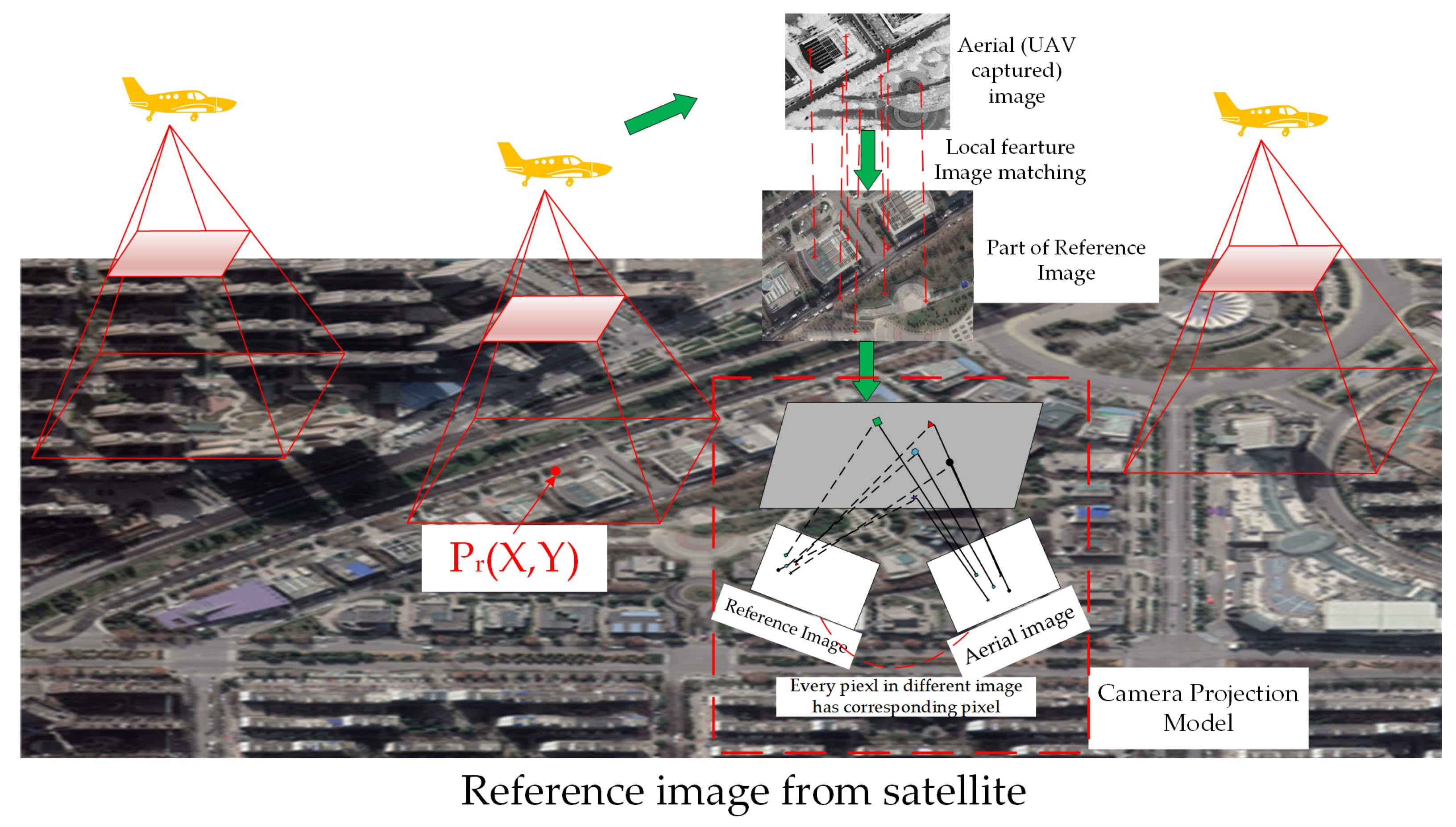
:1. Introduction
- (1)
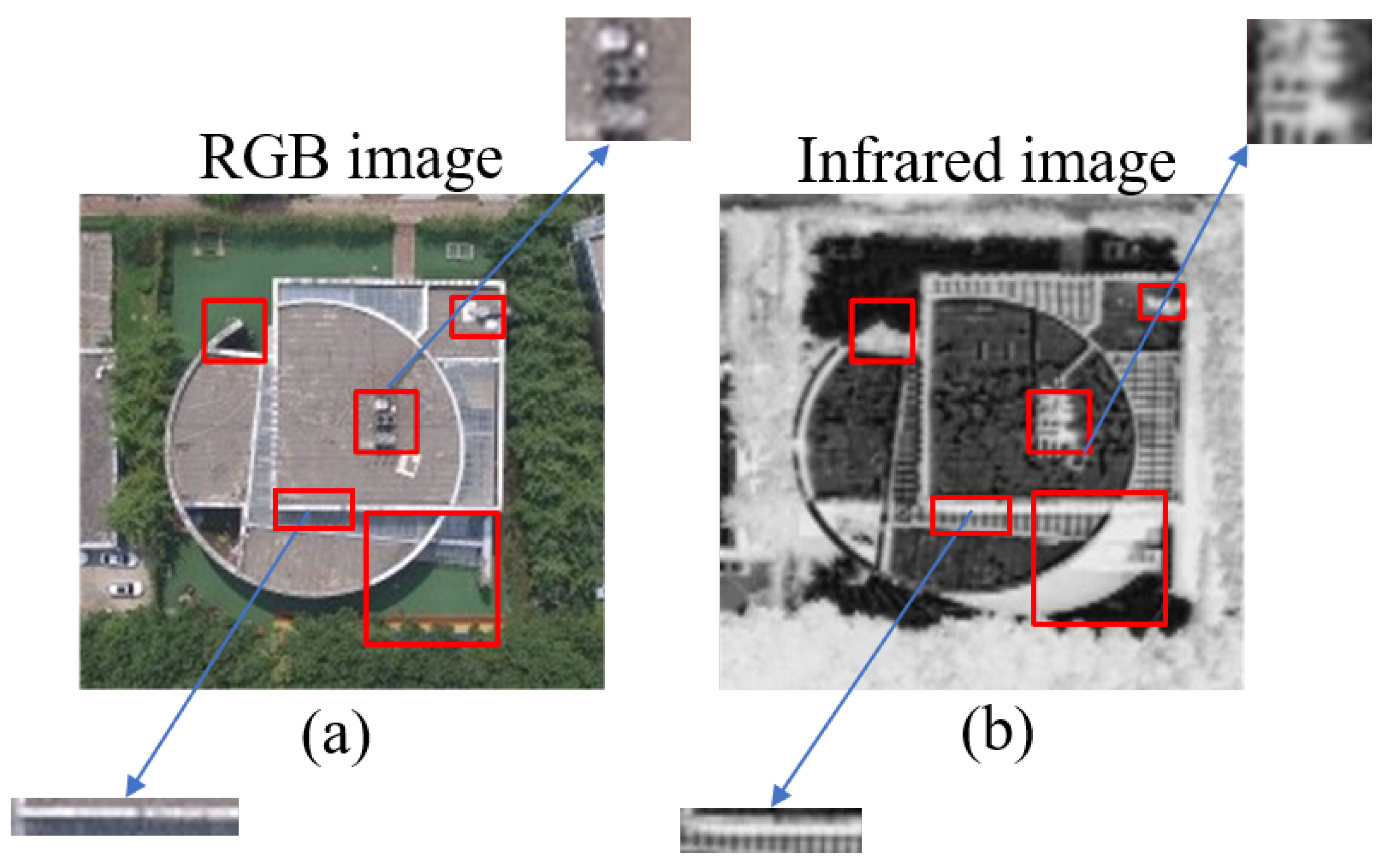
- Even in the same scenes, the different image-forming principles between different types of cameras may cause the same content to be represented by different intensity values, which means that the images from an infrared camera and RGB camera have extreme appearance changes (shown in Figure 2a,b). The poor consistency makes it difficult to find the correspondences based on the traditional image features (such as intensity or gradient values [11,12,13,14]).
- (2)
- In recent years, deep learning techniques have shown the great ability of feature representation in scene matching and other computer vision tasks [15,16,17], which benefits from the explosive growth in image dataset utilization. However, the image datasets for scene matching are almost always from the common cameras (most of them are RGB images from the visual camera). Infrared aerial image and satellite reference image datasets for image matching tasks remain scarce. This is the most significant limitation to application and performance improvement of the deep learning algorithms in this research area.
- (3)
- Even if the infrared aerial images and satellite reference images are sufficient, the learning local feature-based methods still require a large number of labels for algorithm training. Moreover, the labels of local features are difficult to be obtained by human annotation, considering the tremendous numbers and strict requirements of annotation precision. Therefore, there is an urgent need for a method that utilizes the available unlabeled dataset through a self-labeling scheme.
- (1)
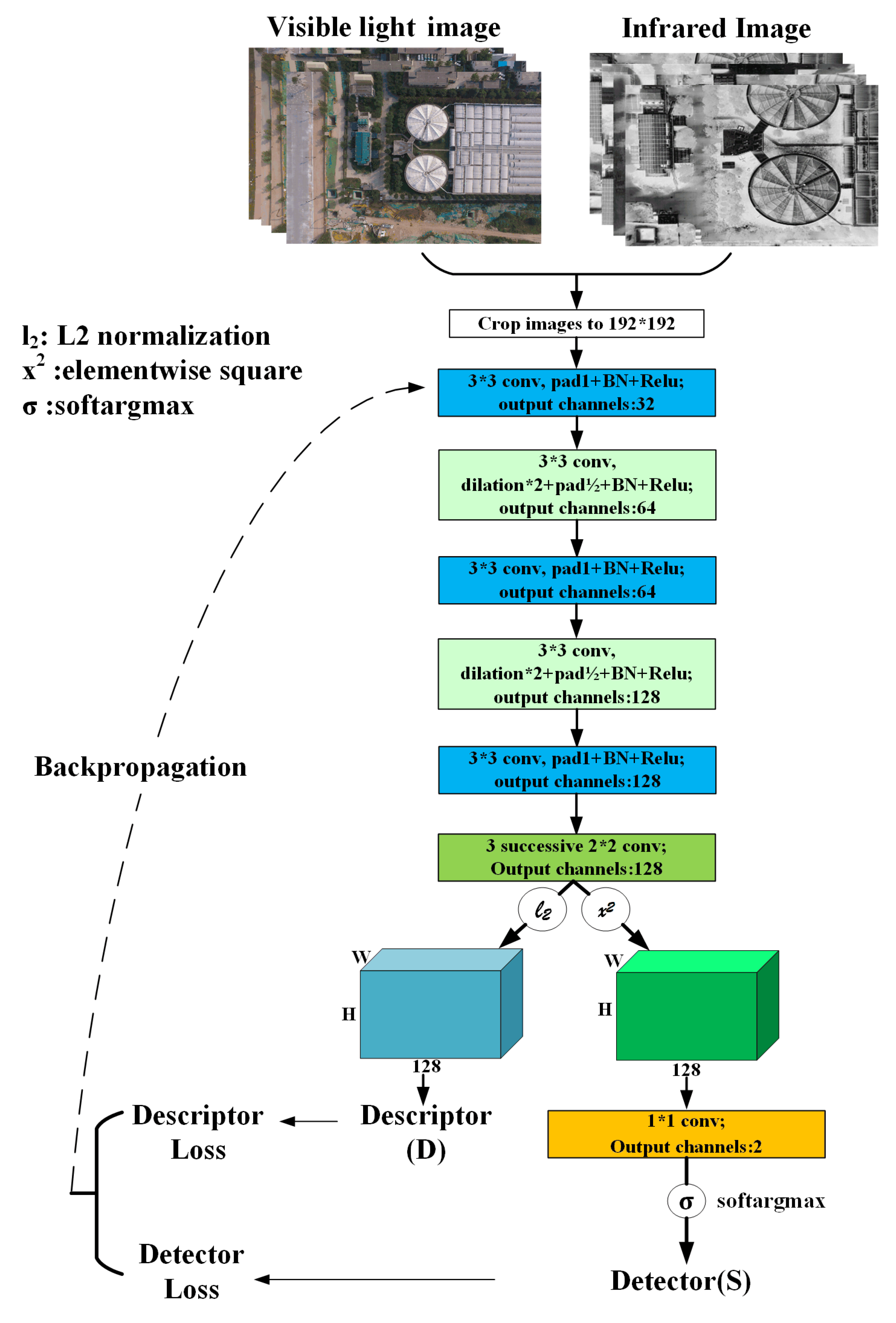
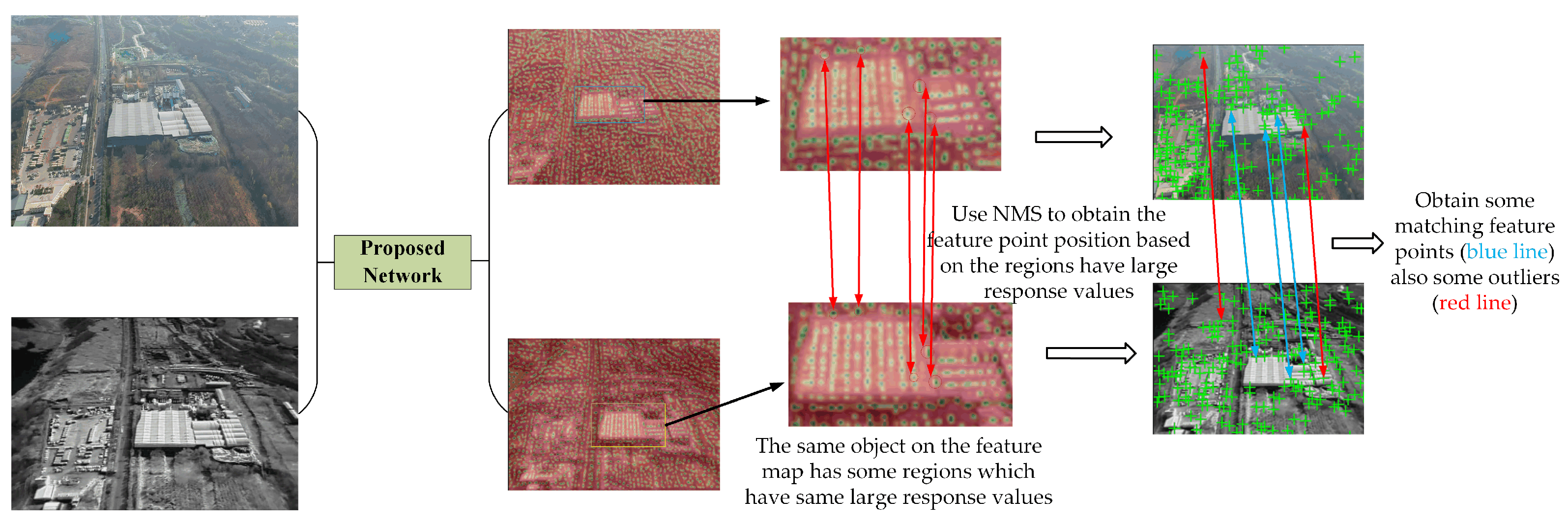
- Our proposed network was established and optimized to achieve a highly precise feature representation and location recognition. Specifically, a backbone network is designed to keep the input resolution consistent, and a novel detector branch with Softargmax is designed to obtain the local maxima in the feature map, which are interest points afterwards. With these improvements, the algorithm can achieve subpixel accuracy for local features detection, which can also improve the self-labeling precision for our iterative training scheme.
- (2)
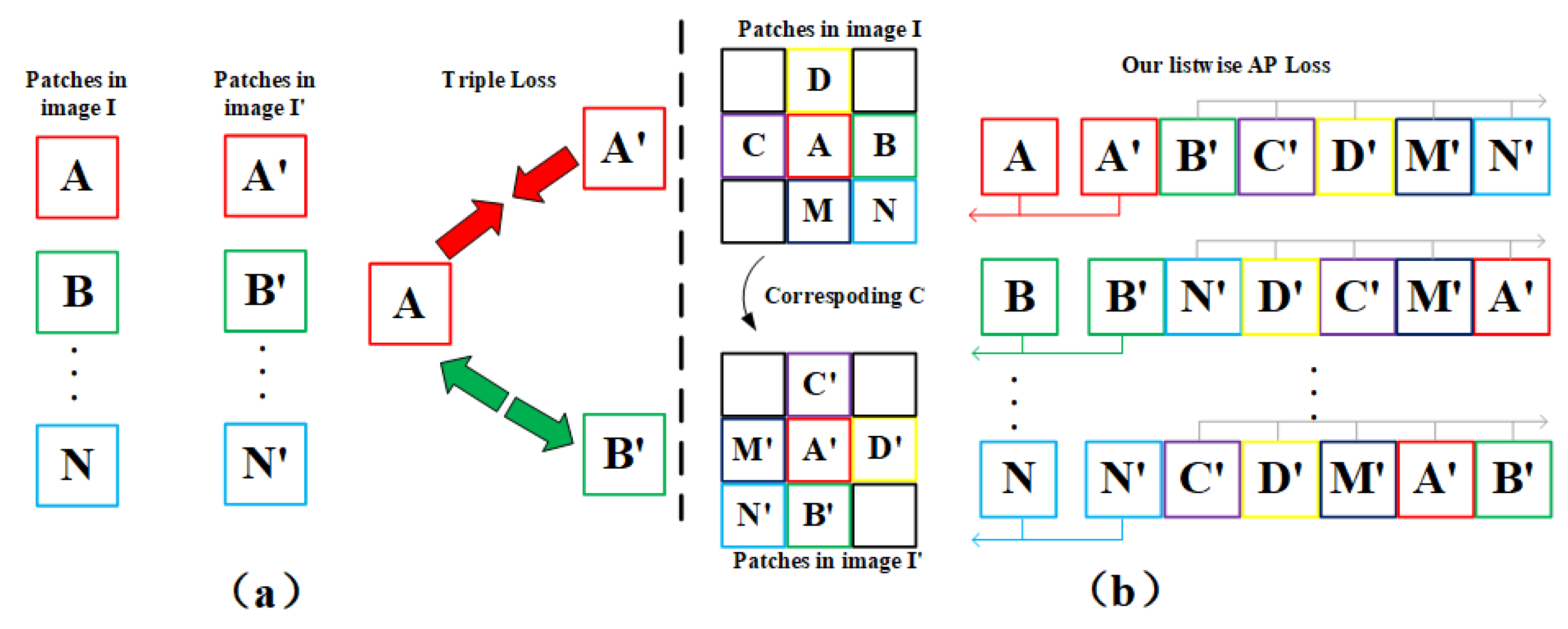
- A novel loss function was proposed for a robust local descriptor to process extreme appearance changes among infrared aerial images and satellite reference images. Unlike the popular loss function that only performs local optimization based on paired or ternary image patches, the novel descriptor loss considers the patches around the interest point and introduces average precision as the global metric for optimization to face the various challenging conditions in place recognition tasks, especially for infrared images and reference images captured from different platforms.
- (3)
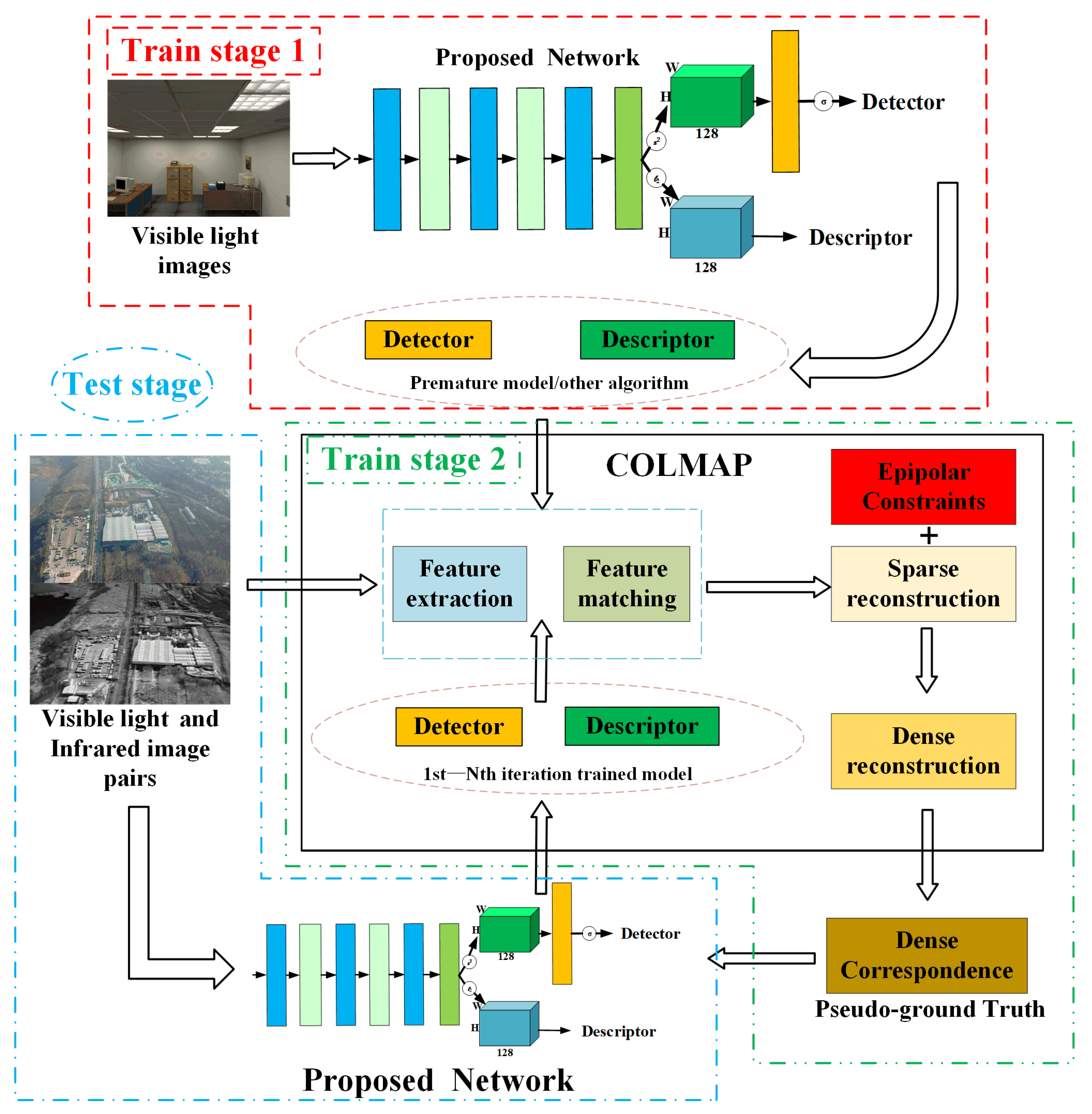
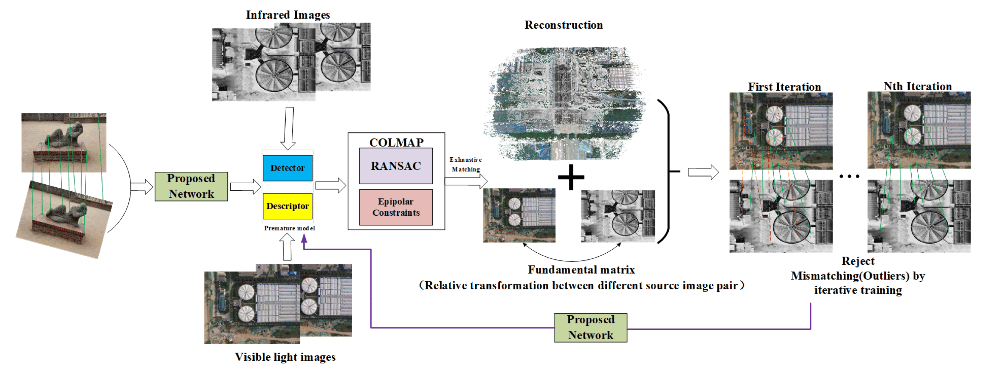
- Owing to the complex collection and a limited number of labeled infrared aerial images and satellite reference images, this paper introduces an iterative training scheme. In the training scheme, we first added geometric constrains using multiple view geometry principles that can autogenerate reliable pseudo-ground truth correspondence from the captured RGB-IR image pairs. Second, the sparse dataset can be reused to iteratively optimize the computing of the correspondence. Benefiting from these processes, the proposed method achieves state-of-the-art performance with the high-quality correspondence as the training pseudo-ground truth.
2. Related Work
2.1. Handcrafted Feature-Based Paradigm
2.2. Learning Feature-Based Paradigm
3. Materials and Methods
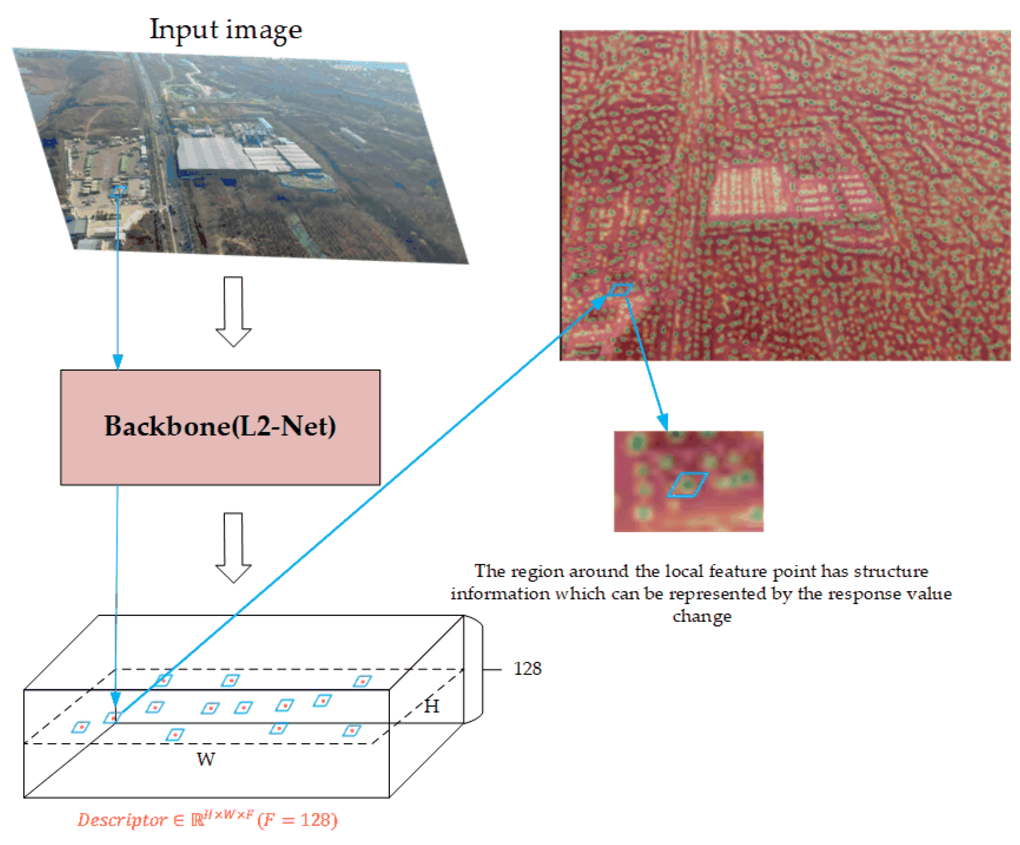
3.1. Learning-Based Detector and Descriptor
3.2. Training Loss
3.3. Implementation Details
3.3.1. Train Scheme
| Algorithm 1 Train stage 1: Self-labelled local feature detector and descriptor model trained on visible light images. |
Input: The visible image I, autogenerated homography matrix: ; Parameters: Interest points function on images: so that and ; Numbers of generated homography matrix: n; Output: Premature local feature detector and descriptor.
|
| Algorithm 2 Train stage 2: Self-labelled local feature detector and descriptor model trained on visible light image and infrared image pairs. |
Input: The visible light image and the infrared image , captured on the same scenes; Parameters: Fundamental matrix as F; every interest point in as and its correspondence point as Output: The local feature detector and descriptor model for RGB-IR image pairs.
|
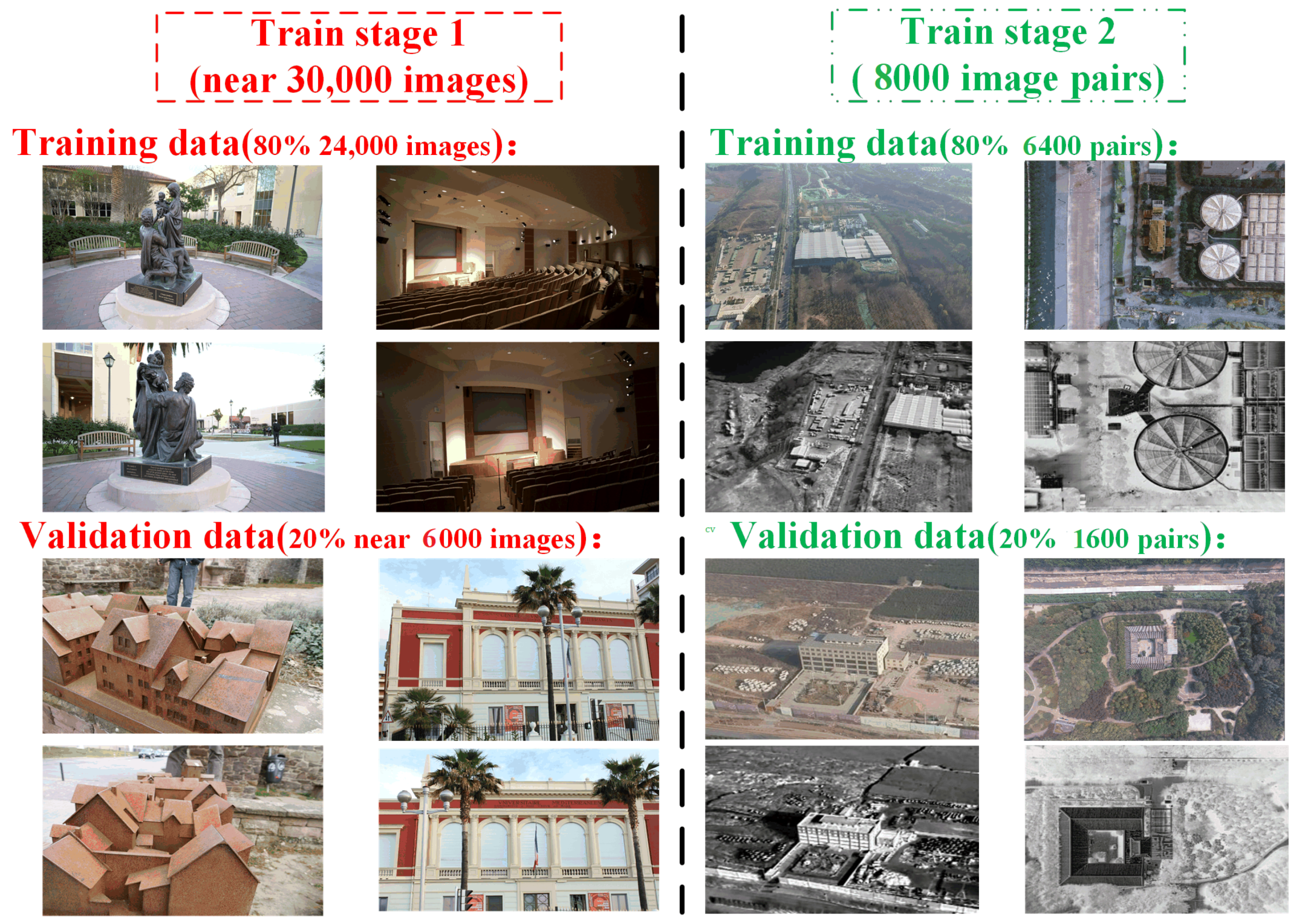
3.3.2. Training Data
3.3.3. Model Training
4. Experiment and Results
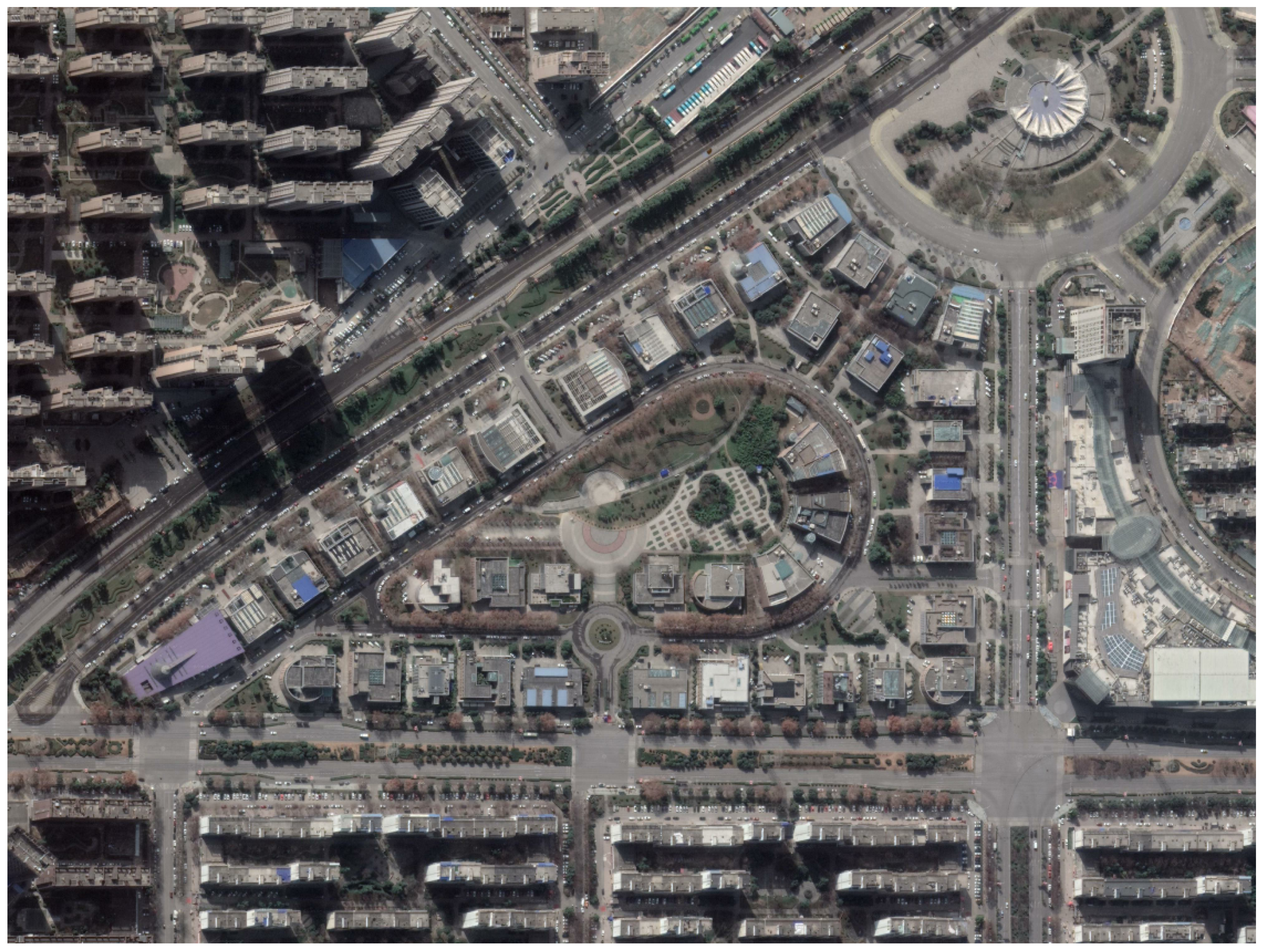
4.1. Experimental Data and Metrics
4.2. Experimental Results of Comparison Methods
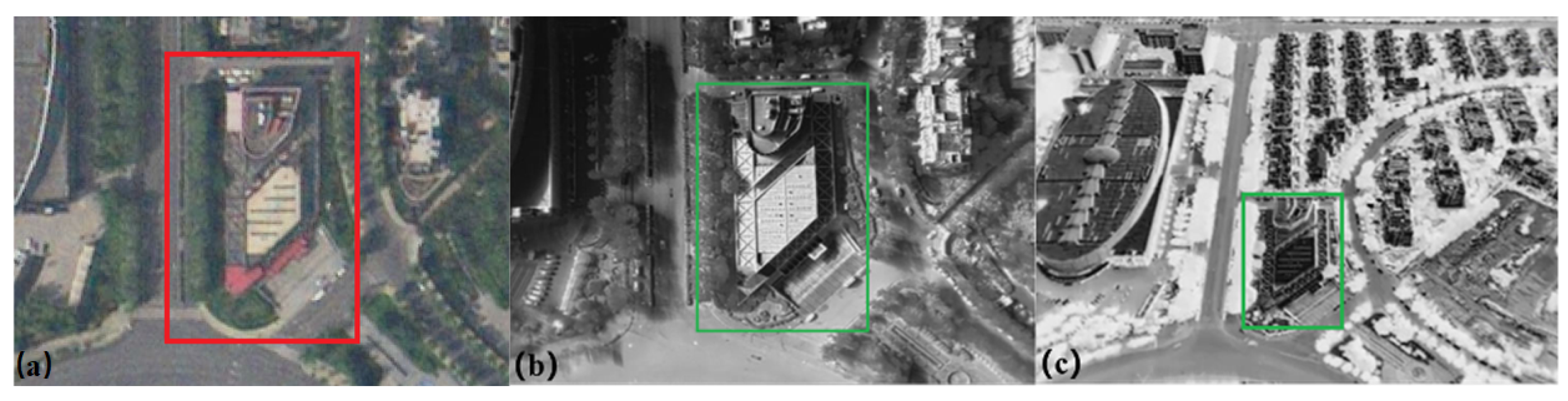
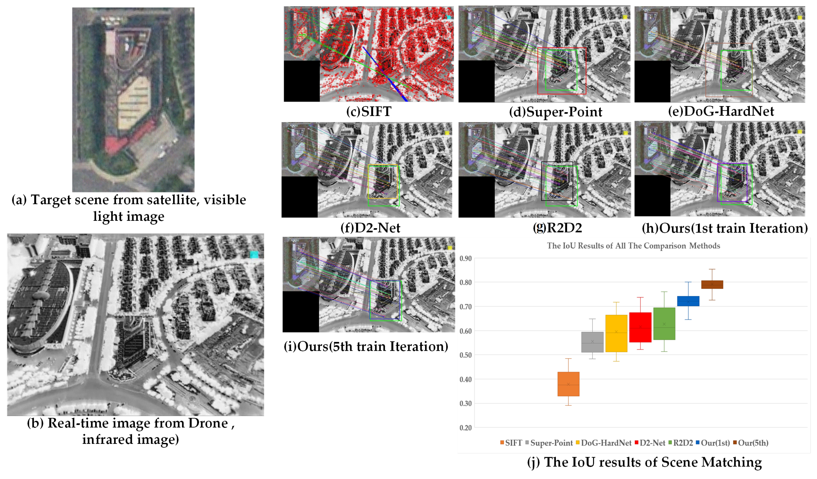
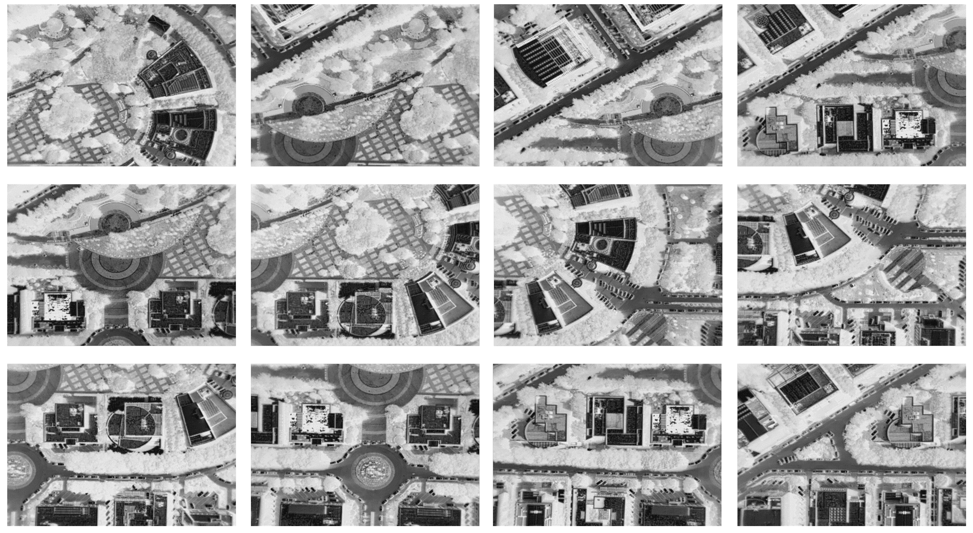
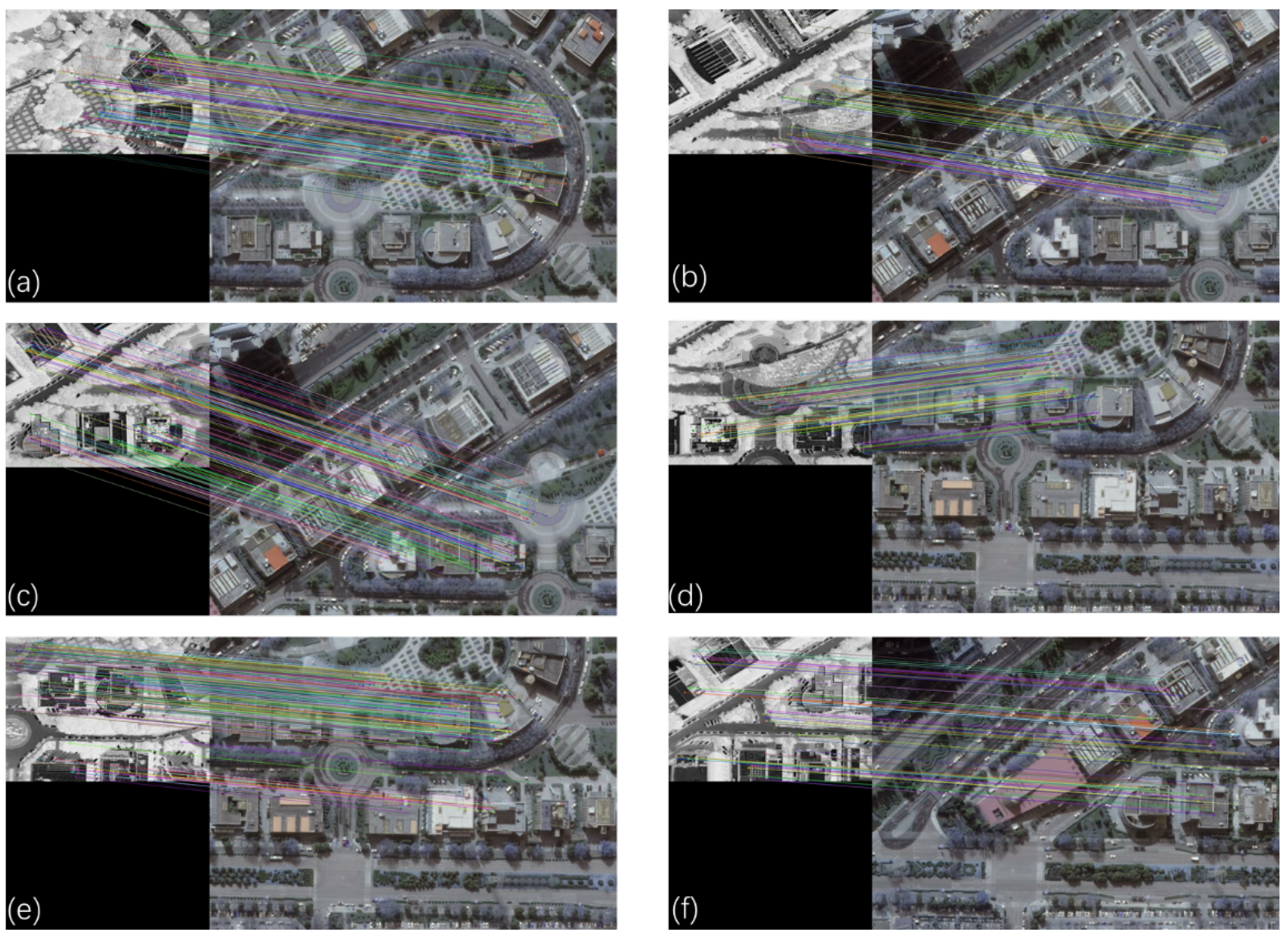
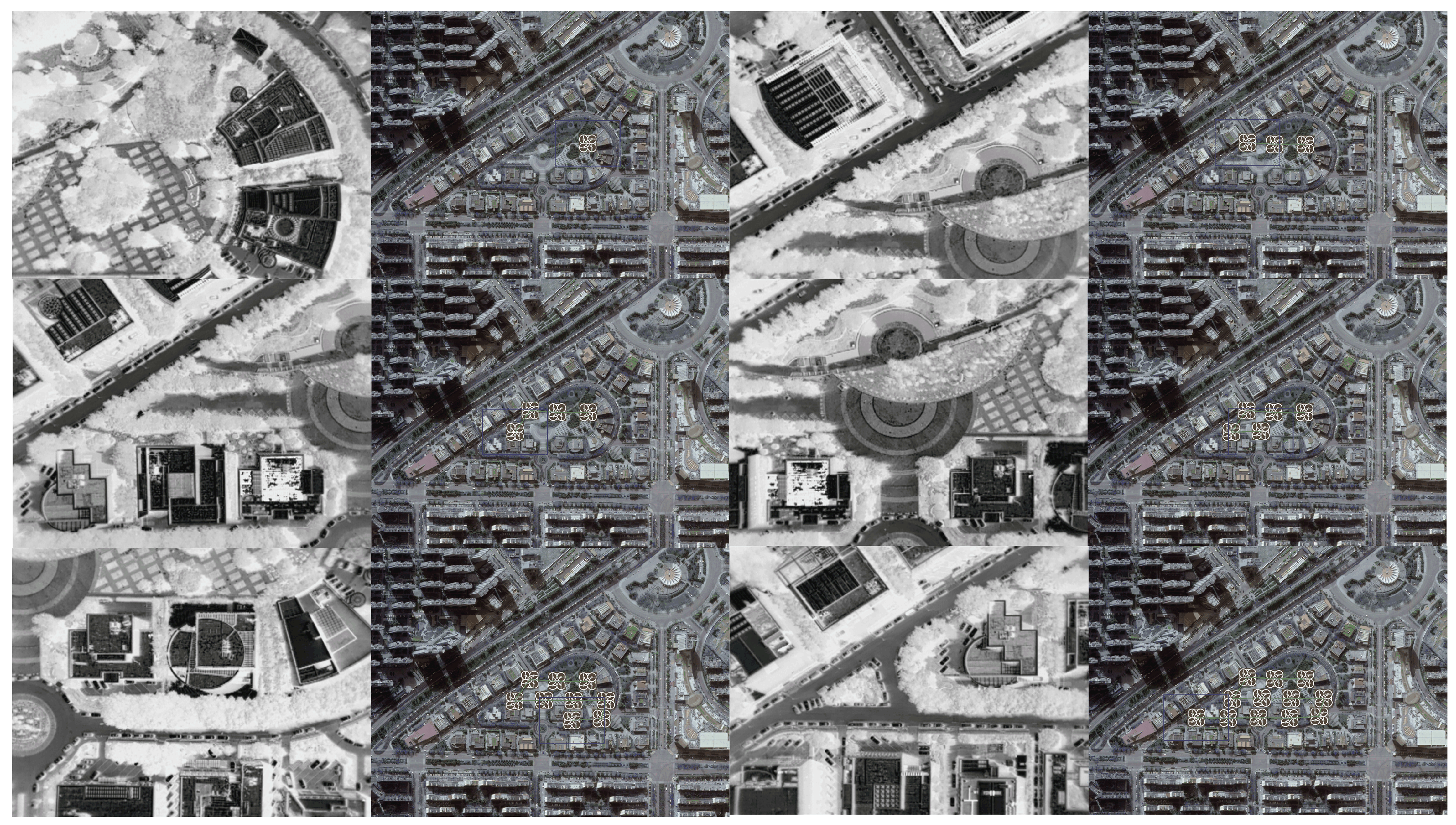
4.3. Applied Experiment
5. Discussion
5.1. Discussion on Experimental Results of the Infrared Aerial Images and Satellite Reference Images
5.2. Discussion on Applied Experimental Results
6. Conclusions
Author Contributions
Funding
Institutional Review Board Statement
Informed Consent Statement
Acknowledgments
Conflicts of Interest
References
- Wang, C.; Peng, T.; Hu, L.; Liu, G. Improved UAV scene matching algorithm based on censure features and FREAK descriptor. In International Conference on Computer Engineering and Networks; Springer: Berlin/Heidelberg, Germany, 2020; pp. 158–167. [Google Scholar]
- Kaniewski, P.; Grzywacz, W. Visual-based navigation system for unmanned aerial vehicles. In Proceedings of the 2017 Signal Processing Symposium (SPSympo), Jachranka Village, Poland, 12–14 September 2017; pp. 1–6. [Google Scholar] [CrossRef]
- Zhuo, X.; Koch, T.; Kurz, F.; Fraundorfer, F.; Reinartz, P. Automatic UAV image geo-registration by matching UAV images to georeferenced image data. Remote Sens. 2017, 9, 376. [Google Scholar] [CrossRef] [Green Version]
- Ebadi, K.; Wood, S. Scene matching-based localization of unmanned aerial vehicles in unstructured environments. In Proceedings of the IEEE 2018 52nd Asilomar Conference on Signals, Systems, and Computers, Pacific Grove, CA, USA, 28–31 October 2018; pp. 1519–1523. [Google Scholar]
- Liu, J.S.; Liu, H.C. Visual Navigation for UAVs Landing on Accessory Building Floor. In Proceedings of the IEEE 2020 International Conference on Pervasive Artificial Intelligence (ICPAI), Taipei, Taiwan, 3–5 December 2020; pp. 158–163. [Google Scholar]
- Andrew, A.M.; Hartley, R. Multiple View Geometry in Computer Vision; Cambridge University Press: Cambridge, UK, 2001. [Google Scholar]
- Conte, G.; Doherty, P. An integrated UAV navigation system based on aerial image matching. In Proceedings of the 2008 IEEE Aerospace Conference, Big Sky, MT, USA, 1–8 March 2008; pp. 1–10. [Google Scholar]
- Balamurugan, G.; Valarmathi, J.; Naidu, V. Survey on UAV navigation in GPS denied environments. In Proceedings of the IEEE 2016 International Conference on Signal Processing, Communication, Power and Embedded System (SCOPES), Odisha, India, 3–5 October 2016; pp. 198–204. [Google Scholar]
- Wan, X.; Liu, J.; Yan, H.; Morgan, G.L. Illumination-invariant image matching for autonomous UAV localisation based on optical sensing. ISPRS J. Photogramm. Remote Sens. 2016, 119, 198–213. [Google Scholar] [CrossRef]
- Carr, J.R.; Sobek, J.S. Digital scene matching area correlator (DSMAC). In Image Processing For Missile Guidance; International Society for Optics and Photonics: Bellingham, WA, USA, 1980; Volume 238, pp. 36–41. [Google Scholar]
- Rublee, E.; Rabaud, V.; Konolige, K.; Bradski, G. ORB: An efficient alternative to SIFT or SURF. In Proceedings of the IEEE 2011 International Conference on Computer Vision, Barcelona, Spain, 6–13 November 2011; pp. 2564–2571. [Google Scholar]
- Bay, H.; Tuytelaars, T.; Van Gool, L. Surf: Speeded up robust features. In European Conference on Computer Vision; Springer: Berlin/Heidelberg, Germany, 2006; pp. 404–417. [Google Scholar]
- Bellavia, F.; Colombo, C. Is there anything new to say about SIFT matching? Int. J. Comput. Vis. 2020, 128, 1–20. [Google Scholar] [CrossRef] [Green Version]
- Lowe, D.G. Distinctive image features from scale-invariant keypoints. Int. J. Comput. Vis. 2004, 60, 91–110. [Google Scholar] [CrossRef]
- Held, D.; Thrun, S.; Savarese, S. Deep learning for single-view instance recognition. arXiv 2015, arXiv:1507.08286. [Google Scholar]
- Han, X.; Leung, T.; Jia, Y.; Sukthankar, R.; Berg, A.C. Matchnet: Unifying feature and metric learning for patch-based matching. In Proceedings of the IEEE Conference on Computer Vision and Pattern Recognition, Boston, MA, USA, 7–12 June 2015; pp. 3279–3286. [Google Scholar]
- Zagoruyko, S.; Komodakis, N. Deep compare: A study on using convolutional neural networks to compare image patches. Comput. Vis. Image Underst. 2017, 164, 38–55. [Google Scholar] [CrossRef]
- Tian, Y.; Fan, B.; Wu, F. L2-net: Deep learning of discriminative patch descriptor in euclidean space. In Proceedings of the IEEE Conference on Computer Vision and Pattern Recognition, Honolulu, HI, USA, 21–26 July 2017; pp. 661–669. [Google Scholar]
- Kern, J.P.; Pattichis, M.S. Robust multispectral image registration using mutual-information models. IEEE Trans. Geosci. Remote Sens. 2007, 45, 1494–1505. [Google Scholar] [CrossRef]
- Lian-Fa, B.; Jing, H.; Yi, Z.; Qian, C. Registration algorithm of infrared and visible images based on improved gradient normalized mutual information and particle swarm optimization. Infrared Laser Eng. 2012, 41, 248–254. [Google Scholar]
- Torabi, A.; Bilodeau, G.A. Local self-similarity-based registration of human ROIs in pairs of stereo thermal-visible videos. Pattern Recognit. 2013, 46, 578–589. [Google Scholar] [CrossRef]
- Bhuiyan, M.A.E.; Witharana, C.; Liljedahl, A.K. Use of Very High Spatial Resolution Commercial Satellite Imagery and Deep Learning to Automatically Map Ice-Wedge Polygons across Tundra Vegetation Types. J. Imaging 2020, 6, 137. [Google Scholar] [CrossRef]
- Zhang, W.; Liljedahl, A.K.; Kanevskiy, M.; Epstein, H.E.; Jones, B.M.; Jorgenson, M.T.; Kent, K. Transferability of the deep learning mask R-CNN model for automated mapping of ice-wedge polygons in high-resolution satellite and UAV images. Remote Sens. 2020, 12, 1085. [Google Scholar] [CrossRef] [Green Version]
- Szeliski, R. Computer Vision: Algorithms and Applications; Springer Science & Business Media: Berlin/Heidelberg, Germany, 2010. [Google Scholar]
- Fischler, M.A.; Bolles, R.C. Random sample consensus: A paradigm for model fitting with applications to image analysis and automated cartography. Commun. ACM 1981, 24, 381–395. [Google Scholar] [CrossRef]
- Yi, K.M.; Trulls, E.; Lepetit, V.; Fua, P. Lift: Learned invariant feature transform. In European Conference on Computer Vision; Springer: Berlin/Heidelberg, Germany, 2016; pp. 467–483. [Google Scholar]
- Noh, H.; Araujo, A.; Sim, J.; Weyand, T.; Han, B. Large-scale image retrieval with attentive deep local features. In Proceedings of the IEEE International Conference on Computer Vision, Venice, Italy, 22–29 October 2017; pp. 3456–3465. [Google Scholar]
- DeTone, D.; Malisiewicz, T.; Rabinovich, A. Superpoint: Self-supervised interest point detection and description. In Proceedings of the IEEE Conference on Computer Vision and Pattern Recognition Workshops, Salt Lake City, UT, USA, 18–22 June 2018; pp. 224–236. [Google Scholar]
- Ono, Y.; Trulls, E.; Fua, P.; Yi, K.M. LF-Net: Learning local features from images. arXiv 2018, arXiv:1805.09662. [Google Scholar]
- Dusmanu, M.; Rocco, I.; Pajdla, T.; Pollefeys, M.; Sivic, J.; Torii, A.; Sattler, T. D2-net: A trainable cnn for joint detection and description of local features. arXiv 2019, arXiv:1905.03561. [Google Scholar]
- Revaud, J.; Weinzaepfel, P.; De Souza, C.; Pion, N.; Csurka, G.; Cabon, Y.; Humenberger, M. R2D2: Repeatable and reliable detector and descriptor. arXiv 2019, arXiv:1906.06195. [Google Scholar]
- Savinov, N.; Seki, A.; Ladicky, L.; Sattler, T.; Pollefeys, M. Quad-networks: Unsupervised learning to rank for interest point detection. In Proceedings of the IEEE Conference on Computer Vision and Pattern Recognition, Honolulu, HI, USA, 21–26 July 2017; pp. 1822–1830. [Google Scholar]
- Zhang, L.; Rusinkiewicz, S. Learning to detect features in texture images. In Proceedings of the IEEE Conference on Computer Vision and Pattern Recognition, Salt Lake City, UT, USA, 18–23 June 2018; pp. 6325–6333. [Google Scholar]
- Simo-Serra, E.; Trulls, E.; Ferraz, L.; Kokkinos, I.; Fua, P.; Moreno-Noguer, F. Discriminative learning of deep convolutional feature point descriptors. In Proceedings of the IEEE International Conference on Computer Vision, Santiago, Chile, 7–13 December 2015; pp. 118–126. [Google Scholar]
- Simonyan, K.; Vedaldi, A.; Zisserman, A. Learning local feature descriptors using convex optimisation. IEEE Trans. Pattern Anal. Mach. Intell. 2014, 36, 1573–1585. [Google Scholar] [CrossRef]
- Mishchuk, A.; Mishkin, D.; Radenovic, F.; Matas, J. Working hard to know your neighbor’s margins: Local descriptor learning loss. arXiv 2017, arXiv:1705.10872. [Google Scholar]
- Schonberger, J.L.; Frahm, J.M. Structure-from-motion revisited. In Proceedings of the IEEE Conference on Computer Vision and Pattern Recognition, Las Vegas, NV, USA, 27–30 June 2016; pp. 4104–4113. [Google Scholar]
- Fisher, A.; Cannizzaro, R.; Cochrane, M.; Nagahawatte, C.; Palmer, J.L. ColMap: A memory-efficient occupancy grid mapping framework. Robot. Auton. Syst. 2021, 142, 103755. [Google Scholar] [CrossRef]
- Ma, J.; Jiang, X.; Fan, A.; Jiang, J.; Yan, J. Image matching from handcrafted to deep features: A survey. Int. J. Comput. Vis. 2021, 129, 23–79. [Google Scholar] [CrossRef]
- Revaud, J.; Almazán, J.; Rezende, R.S.; Souza, C.R.D. Learning with average precision: Training image retrieval with a listwise loss. In Proceedings of the IEEE/CVF International Conference on Computer Vision, Seoul, Korea, 27–28 October 2019; pp. 5107–5116. [Google Scholar]
- Burges, C.; Shaked, T.; Renshaw, E.; Lazier, A.; Deeds, M.; Hamilton, N.; Hullender, G. Learning to rank using gradient descent. In Proceedings of the 22nd International Conference on Machine Learning, Bonn, Germany, 7–11 August 2005; pp. 89–96. [Google Scholar]
- Cao, Z.; Qin, T.; Liu, T.Y.; Tsai, M.F.; Li, H. Learning to rank: From pairwise approach to listwise approach. In Proceedings of the 24th International Conference on Machine Learning, Corvallis, OR, USA, 20–24 June 2007; pp. 129–136. [Google Scholar]
- He, K.; Lu, Y.; Sclaroff, S. Local descriptors optimized for average precision. In Proceedings of the IEEE Conference on Computer Vision and Pattern Recognition, Salt Lake City, UT, USA, 18–23 June 2018; pp. 596–605. [Google Scholar]
- Cakir, F.; He, K.; Xia, X.; Kulis, B.; Sclaroff, S. Deep metric learning to rank. In Proceedings of the IEEE/CVF Conference on Computer Vision and Pattern Recognition, Long Beach, CA, USA, 15–20 June 2019; pp. 1861–1870. [Google Scholar]
- Lin, T.Y.; Maire, M.; Belongie, S.; Hays, J.; Perona, P.; Ramanan, D.; Dollár, P.; Zitnick, C.L. Microsoft coco: Common objects in context. In European Conference on Computer Vision; Springer: Berlin/Heidelberg, Germany, 2014; pp. 740–755. [Google Scholar]
- Li, Z.; Snavely, N. Megadepth: Learning single-view depth prediction from internet photos. In Proceedings of the IEEE Conference on Computer Vision and Pattern Recognition, Salt Lake City, UT, USA, 18–23 June 2018; pp. 2041–2050. [Google Scholar]
- Radiuk, P.M. Impact of training set batch size on the performance of convolutional neural networks for diverse datasets. Inf. Technol. Manag. Sci. 2017, 20, 20–24. [Google Scholar] [CrossRef]
- You, K.; Long, M.; Wang, J.; Jordan, M.I. How does learning rate decay help modern neural networks? arXiv 2019, arXiv:1908.01878. [Google Scholar]
- Ge, R.; Kakade, S.M.; Kidambi, R.; Netrapalli, P. The step decay schedule: A near optimal, geometrically decaying learning rate procedure for least squares. arXiv 2019, arXiv:1904.12838. [Google Scholar]
- Mishra, P. Supervised Learning Using PyTorch. In PyTorch Recipes; Springer: Berlin/Heidelberg, Germany, 2019; pp. 127–149. [Google Scholar]
- Lewkowycz, A. How to decay your learning rate. arXiv 2021, arXiv:2103.12682. [Google Scholar]


| Method | Handcrafted Feature | Learning Feature |
|---|---|---|
| subpixel accuracy | high-level feature | |
| Advantage | high speed | repeatable and reliable |
| data efficient | discriminability and robustness | |
| low-order feature detectors | require large amount of labelled data | |
| Disadvantage | require good modeling | efficiency depend on structure |
| bad robust for apparent variance | generality only in trained regime |
| Dataset for Train Stage | Source | Number of Images | Resolution |
|---|---|---|---|
| MS-COCO [45] | near 30,000 images | ||
| Train Stage 1 | 80% for training | ||
| MegaDepth [46] | 20% for training | ||
| RGB images from satellite | 8000 image pairs | ||
| Train Stage 2 | RGB images from UAV | 80% for training | |
| infrared images from UAV | 20% for training |
| Viewpoint Change (deg) | 0/30/45 | 0/30/45 | 0/30/45 |
|---|---|---|---|
| Method | Precision (%) | Recall (%) | F1-Score |
| SIFT [14] | 33.2/19.6/8.7 | 10.1/9.9/5.3 | 15.5/13.2/6.6 |
| DoG-HardNet [36] | 71.2/65.1/48.7 | 65.2/61.6/41.7 | 68.1/63.3/44.9 |
| Super-Point [28] | 69.1/64.5/43.9 | 59.8/55.3/40.1 | 64.1/59.5/41.9 |
| D2-Net [30] | 78.4/56.3/40.3 | 68.7/56.7/37.8 | 73.2/56.5/39.0 |
| R2D2 [31] | 77.6/65.4/45.6 | 67.3/62.5/42.4 | 72.1/63.9/43.9 |
| Our Method (1st train Iteration) | 78.5/64.1/49.3 | 68.9/60.8/46.3 | 73.4/62.4/47.8 |
| Our Method (5th train Iteration) | 81.2/66.3/50.4 | 72.3/63.1/48.7 | 76.5/64.7/49.5 |
| Viewpoint Change (deg) | 0/30/45 | 0/30/45 | 0/30/45 |
|---|---|---|---|
| Method | Precision (%) | Recall (%) | F1-Score |
| SIFT [14] | 26.8/16.6/5.7 | 8.7/4.5/2.2 | 13.1/7.0/3.2 |
| DoG-HardNet [36] | 50.5/41.4/34.7 | 43.7/39.8/32.6 | 46.9/40.6/33.6 |
| Super-Point [28] | 50.3/41.1/33.9 | 40.0/37.1/29.4 | 44.6/39.0/31.5 |
| D2-Net [30] | 52.5/39.0/32.2 | 46.0/38.2/27.0 | 49.0/38.6/29.8 |
| R2D2 [31] | 51.2/40.9/33.8 | 45.1/39.2/30.6 | 48.0/40.0/32.1 |
| Our Method (1st train Iteration) | 53.7/42.5/35.6 | 48.3/41.9/33.7 | 50.9/42.2/34.6 |
| Our Method (5th train Iteration) | 56.4/42.7/36.9 | 50.4/42.3/35.2 | 53.2/42.5/36.0 |
| Samples in Figure 10 | SIFT [14] (RMSE/LE) | DoG-Hard [36] (RMSE/LE) | Super-Point [28] (RMSE/LE) | D2-Net [30] (RMSE/LE) | R2D2 [31] (RMSE/LE) | Our Method |
|---|---|---|---|---|---|---|
| (a) | —/— | —/— | —/— | 3.40/7.16 | 2.14/4.32 | 1.69/3.61 |
| (b) | 2.11/4.29 | 3.31/7.09 | 4.51/8.69 | 5.14/10.23 | 2.35/4.81 | 2.04/4.15 |
| (c) | 1.76/3.17 | 2.76/5.71 | 2.78/5.63 | 3.51/7.93 | 1.98/3.88 | 0.82/1.92 |
| (d) | —/— | —/— | —/— | 6.71/13.43 | 5.62/11.27 | 3.97/7.78 |
| (e) | —/— | 4.18/8.63 | 5.27/12.11 | 5.73/12.13 | 3.53/7.12 | 2.44/5.03 |
| (f) | —/— | 4.74/9.66 | 6.25/12.98 | 6.31/13.03 | 4.84/9.25 | 3.71/7.34 |
Publisher’s Note: MDPI stays neutral with regard to jurisdictional claims in published maps and institutional affiliations. |
© 2021 by the authors. Licensee MDPI, Basel, Switzerland. This article is an open access article distributed under the terms and conditions of the Creative Commons Attribution (CC BY) license (https://creativecommons.org/licenses/by/4.0/).
Share and Cite
Zhang, X.; He, Z.; Ma, Z.; Wang, Z.; Wang, L. LLFE: A Novel Learning Local Features Extraction for UAV Navigation Based on Infrared Aerial Image and Satellite Reference Image Matching. Remote Sens. 2021, 13, 4618. https://0-doi-org.brum.beds.ac.uk/10.3390/rs13224618
Zhang X, He Z, Ma Z, Wang Z, Wang L. LLFE: A Novel Learning Local Features Extraction for UAV Navigation Based on Infrared Aerial Image and Satellite Reference Image Matching. Remote Sensing. 2021; 13(22):4618. https://0-doi-org.brum.beds.ac.uk/10.3390/rs13224618
Chicago/Turabian StyleZhang, Xupei, Zhanzhuang He, Zhong Ma, Zhongxi Wang, and Li Wang. 2021. "LLFE: A Novel Learning Local Features Extraction for UAV Navigation Based on Infrared Aerial Image and Satellite Reference Image Matching" Remote Sensing 13, no. 22: 4618. https://0-doi-org.brum.beds.ac.uk/10.3390/rs13224618