Article

Mapping Relict Charcoal Hearths in New England Using Deep Convolutional Neural Networks and LiDAR Data

1
Department of Geography, University of Connecticut, Storrs, CT 06269, USA
2
Department of Geosciences, University of Connecticut, Storrs, CT 06269, USA
3
North Carolina Institute for Climate Studies, North Carolina State University, Asheville, NC 28801, USA
4
Department of Natural Resources and the Environment, University of Connecticut, Storrs, CT 06269, USA
*
Author to whom correspondence should be addressed.
Remote Sens. 2021, 13(22), 4630; https://0-doi-org.brum.beds.ac.uk/10.3390/rs13224630
Submission received: 13 October 2021 / Revised: 12 November 2021 / Accepted: 13 November 2021 / Published: 17 November 2021

Abstract

:
Advanced deep learning methods combined with regional, open access, airborne Light Detection and Ranging (LiDAR) data have great potential to study the spatial extent of historic land use features preserved under the forest canopy throughout New England, a region in the northeastern United States. Mapping anthropogenic features plays a key role in understanding historic land use dynamics during the 17th to early 20th centuries, however previous studies have primarily used manual or semi-automated digitization methods, which are time consuming for broad-scale mapping. This study applies fully-automated deep convolutional neural networks (i.e., U-Net) with LiDAR derivatives to identify relict charcoal hearths (RCHs), a type of historical land use feature. Results show that slope, hillshade, and Visualization for Archaeological Topography (VAT) rasters work well in six localized test regions (spatial scale: <1.5 km2, best F1 score: 95.5%), but also at broader extents at the town level (spatial scale: 493 km2, best F1 score: 86%). The model performed best in areas with deciduous forest and high slope terrain (e.g., >15 degrees) (F1 score: 86.8%) compared to coniferous forest and low slope terrain (e.g., <15 degrees) (F1 score: 70.1%). Overall, our results contribute to current methodological discussions regarding automated extraction of historical cultural features using deep learning and LiDAR.

1. Introduction

Relict charcoal hearths (RCHs) and charcoal production provide a unique insight into the economic history and historic land use of New England, a region in the northeastern United States [1]. Charcoal was primarily used from the mid-18th through the early 20th century in the northeastern U.S to produce the fuel needed to process mined iron [2,3,4,5]. RCH distribution varies throughout the region from high densities (e.g., >100 per km2), typically near iron furnaces, to much lower densities or sporadic (e.g., <5 per km2) where charcoal was produced for local subsistence trade by farmers and foresters [3]. Large scale charcoal production took place in the northwestern portion of Connecticut, a state in southern New England, between 1760 and 1920 in support of the Salisbury Iron District [1,6]. In this region, the distribution and spatial extent of RCHs have been used to understand economic history and reconstruct historic land use.
High-resolution airborne light detection and ranging (LiDAR) data play an essential role in visualizing morphological features or anthropogenic features on landscapes at global scales and can be used effectively in New England to identify a type of historical land use feature which has been variously called a charcoal hearth or charcoal kiln [1,4,7,8,9,10,11]. Digital Elevation Models (DEMs) derived from LiDAR point clouds can provide morphological information at fine scales under dense forest canopies, and for this reason have been widely used to identify various types of historical land use features on a global scale [4,8,12,13]. In addition, a diverse range of visualization techniques for LiDAR data have been employed, which has allowed for detection of morphological features on LiDAR-derived rasters including slope, hillshade, or blended imagery, such as Principal Component Analysis (PCA) of hillshades, sky-view factor, and openness models and simplified local relief model (SLRM) which are all popular visualization methods to highlight morphological properties of features [14,15,16,17,18,19,20].
The current widespread availability of LiDAR data in addition to a diverse range of visualization techniques have allowed several (semi-) automated feature extraction techniques to be explored such as template-matching [21], object-based image analysis (OBIA) [7], machine learning (ML) [22,23], and deep learning (DL) [9,10,11,12,24,25,26]; all of which have been applied to morphological feature extraction. When it comes to mapping at regional scales, these approaches enhance the time-consuming nature of on-screen manual digitization. Template-matching and OBIA are semi-automated approaches based on a ruleset built by geometric or morphological characteristics, such as length, area, and slope angle of feature. ML is another semi-automated method based on the statistical relationship among training datasets. Unlike these three approaches, DL is a fully-automated approach as long as training data are available. A number of studies have focused on the application of different DL models for anthropogenic feature detection recently [9,10,11,24,25]. In this study, two main groups of DL models were used: (1) object detection models (i.e., R-CNN, Faster R-CNN) and (2) semantic segmentation models (i.e., U-Net, ResUnet, and FCN). Object detection models detect the extent of a target object with a bounding box. Semantic segmentation models define semantic regions and segment these regions into classes (e.g., target object vs. background). These methods have been applied to identifying archaeological features [9,10,11,24].
The application of DL to detect anthropogenic features representative of historic land use practices such as RCHs in New England provides great potential to understand a unique land use history as well as define the extent of historic charcoal production, which is representative of widespread deforestation in the region, between the 18th to mid-20th centuries. To date, most studies in this region have only used manual digitization techniques [8] or OBIA techniques [7] for extracting historical land use features from LiDAR data. The present regional coverage of LiDAR data provides an opportunity for efficient automated mapping at much broader scales to quantify the impacts of historic land use more easily. Therefore, this study aims to (1) develop fully automated extraction of anthropogenic features (i.e., RCHs) in southern New England using high-resolution airborne LiDAR and deep convolutional neural networks, (2) evaluate model performance in different terrain and landscape scenarios, and (3) discuss implications for historic landscape dynamics in this region.

2. Materials and Methods
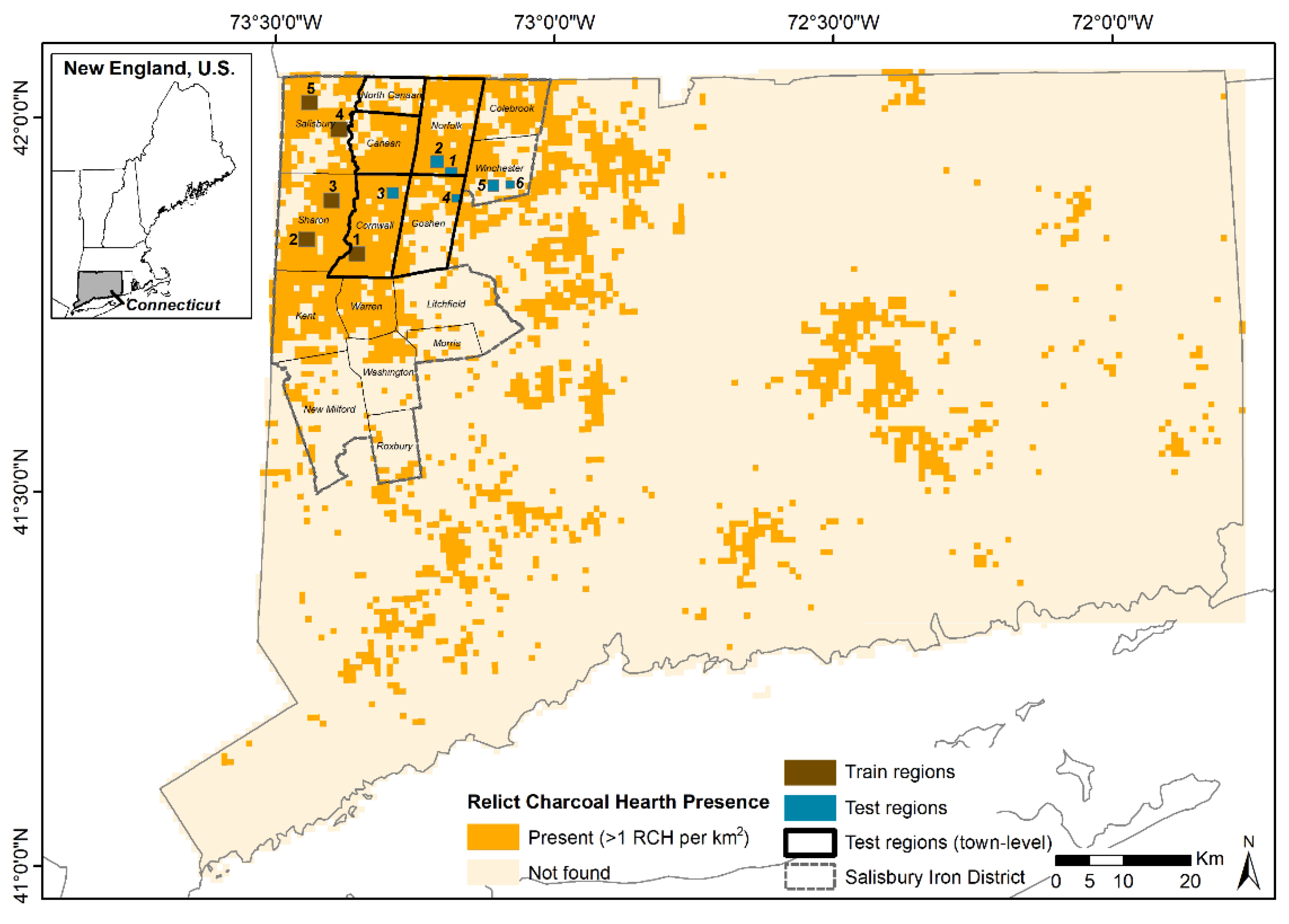
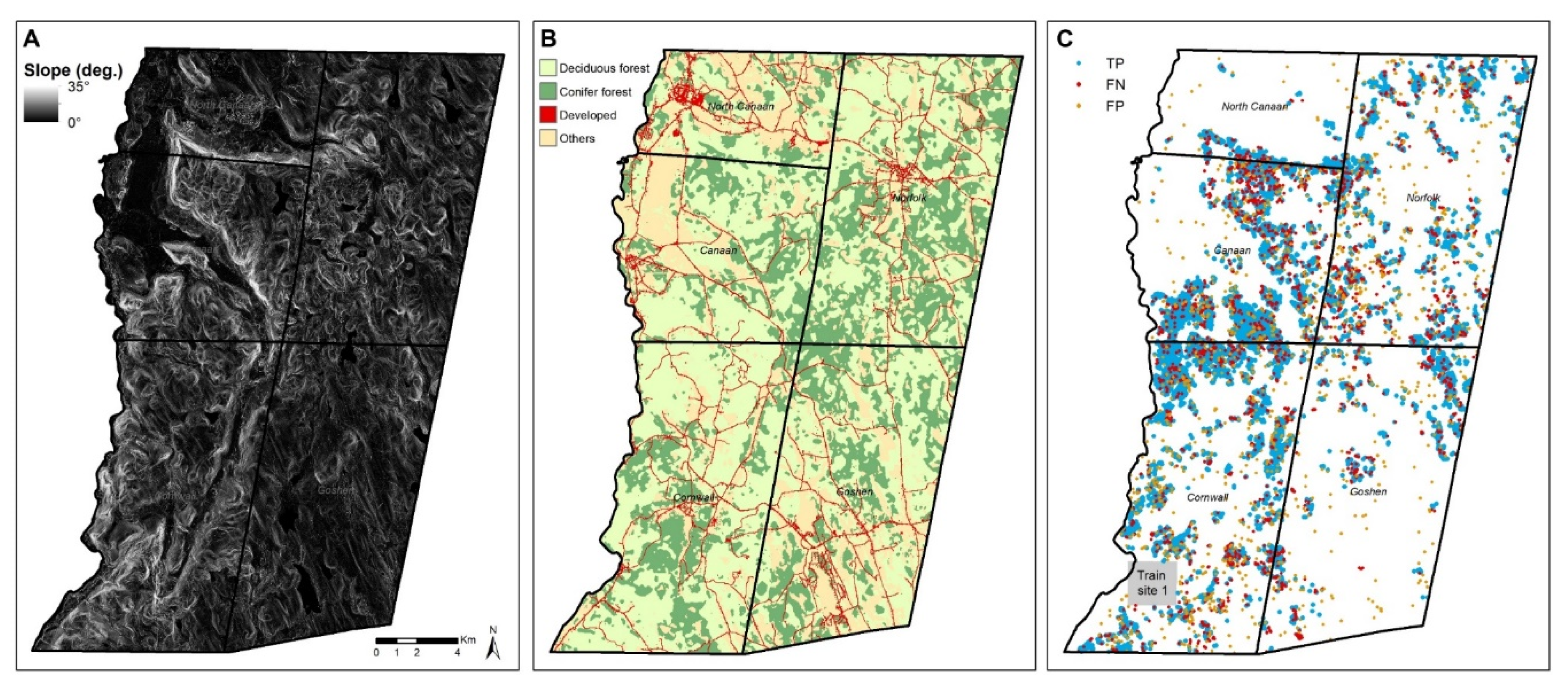
2.1. Study Area

The study areas are located in Litchfield County, Connecticut, in a part of the northeastern United States called New England. Much of the northeastern U.S. participated in the iron industry during the 19th century [27] and the northwestern portion of Connecticut, historically called the Salisbury Iron District, was well-known and prosperous during that time period [1]. Production of charcoal for iron furnaces in the region resulted in RCH construction across this landscape. RCHs are extant on the landscape in large quantities and visible in LiDAR derivatives. These features are representative of the widespread historical deforestation in the region, and are now covered with a dense forest canopy consisting of deciduous forest and northern hardwoods [28]. Five training regions were placed in a high-density area where there was an RCH presence of at least 1 RCH per km2 (Figure 1). These training regions contained a total of 1700 RCHs which are easily identifiable in a LiDAR-derived slope map. To evaluate the trained model, six test regions were selected across rugged and smooth terrain, and various land cover types such as deciduous and coniferous forest, cleared fields, and developed (Table 1).

2.2. Data Description

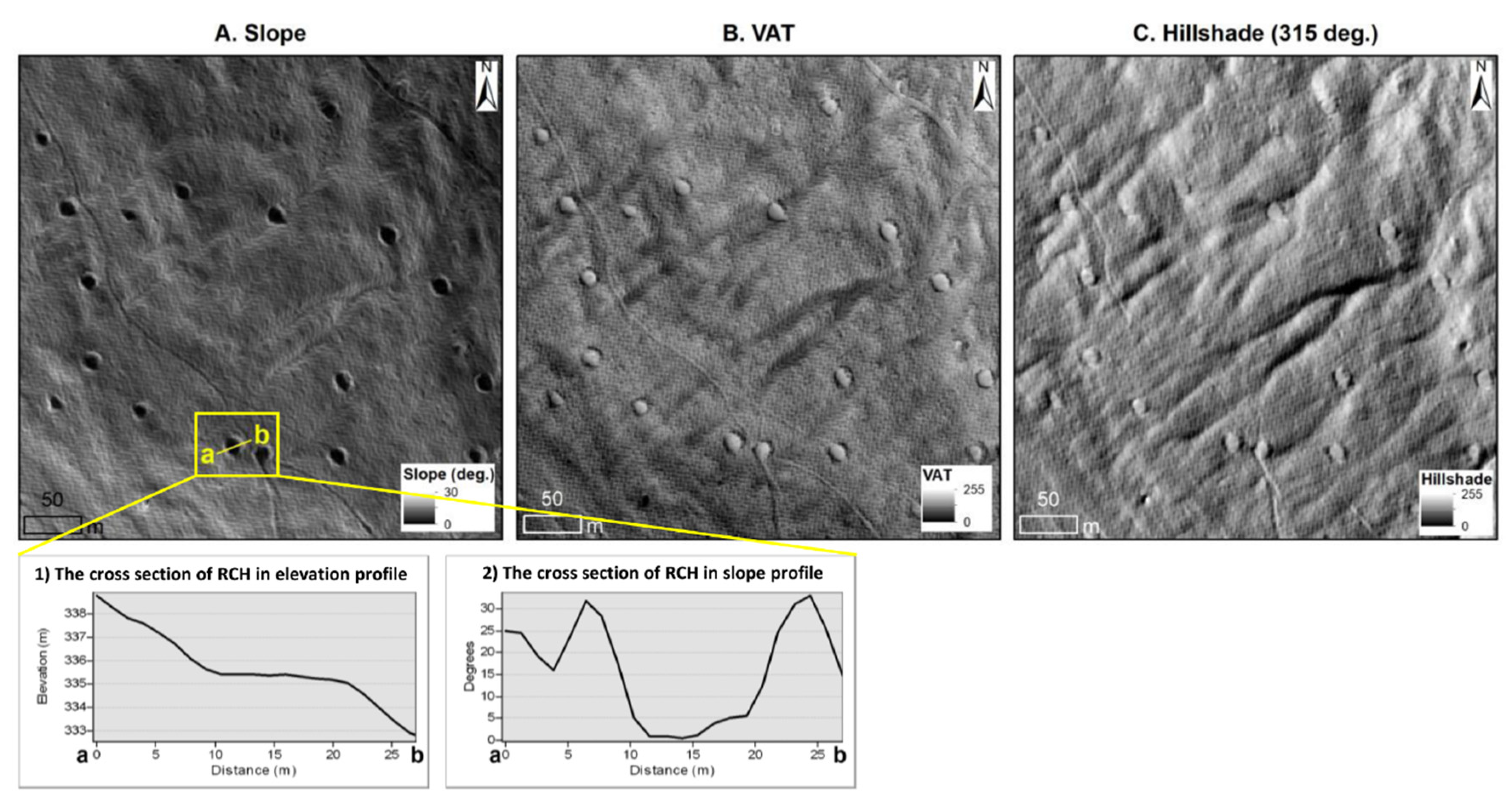
2.2.1. LiDAR Data and Derivatives

In this study, 1 m high-resolution LiDAR DEMs were used to prepare the input image datasets for the U-Net model as well as a reference dataset based on on-screen manual digitization. The DEMs used were produced from the ground classified points of two different LiDAR point cloud datasets, one flown in 2011 and one in 2016 [30,31]. Both datasets were collected in the spring after snow had melted and when deciduous trees were without leaves. The point spacing of 2011 LiDAR data was no greater than 1 point every 0.7 m [31] and the point density of 2016 LiDAR data was 2 points per square meter [30]. The quality of LiDAR point clouds and subsequent DEM tiles can be influenced by the forest canopy type (i.e., deciduous vs. coniferous) and underlying vegetation, since it is difficult to discern low vegetation points from the ground surface. Overall, these data quality issues may lead to lower point densities for ground-classified points, which can create small blurred areas in the interpolated DEM and make interpretation more difficult [4,32,33]. After being downloaded from [34], the necessary DEM tiles were mosaicked using ArcGIS Pro to cover the five training regions and six test regions.
With the high spatial resolution of the data and distinct morphological characteristics, RCHs are clearly identifiable in LiDAR derivatives, such as slope, VAT (Visualization for Archaeological Topography tool) [35], and hillshade rasters (Figure 2). First, a slope raster was produced using the ArcGIS Pro Slope tool and it worked well with the morphology of RCHs which have low slopes in the center and an adjacent high-slope edge (Figure 2A). Second, we used the Relief Visualization Toolbox (RVT) [36,37] to create a single channel VAT raster. The VAT raster is an alternative hillshaded DEM for visualizing landform features proposed by Verbovšek et al. (2019) [35]. It is produced by blending four different rasters such as slope and hillshade, sky-view factor [37], and positive openness [35]. As shown in Figure 2B, it is effective at capturing the circular nature of the RCHs, and the edge of each RCH is distinguishable from the background. Last, a hillshade map with a different azimuth angle was generated using the Hillshade tool in ArcGIS Pro.

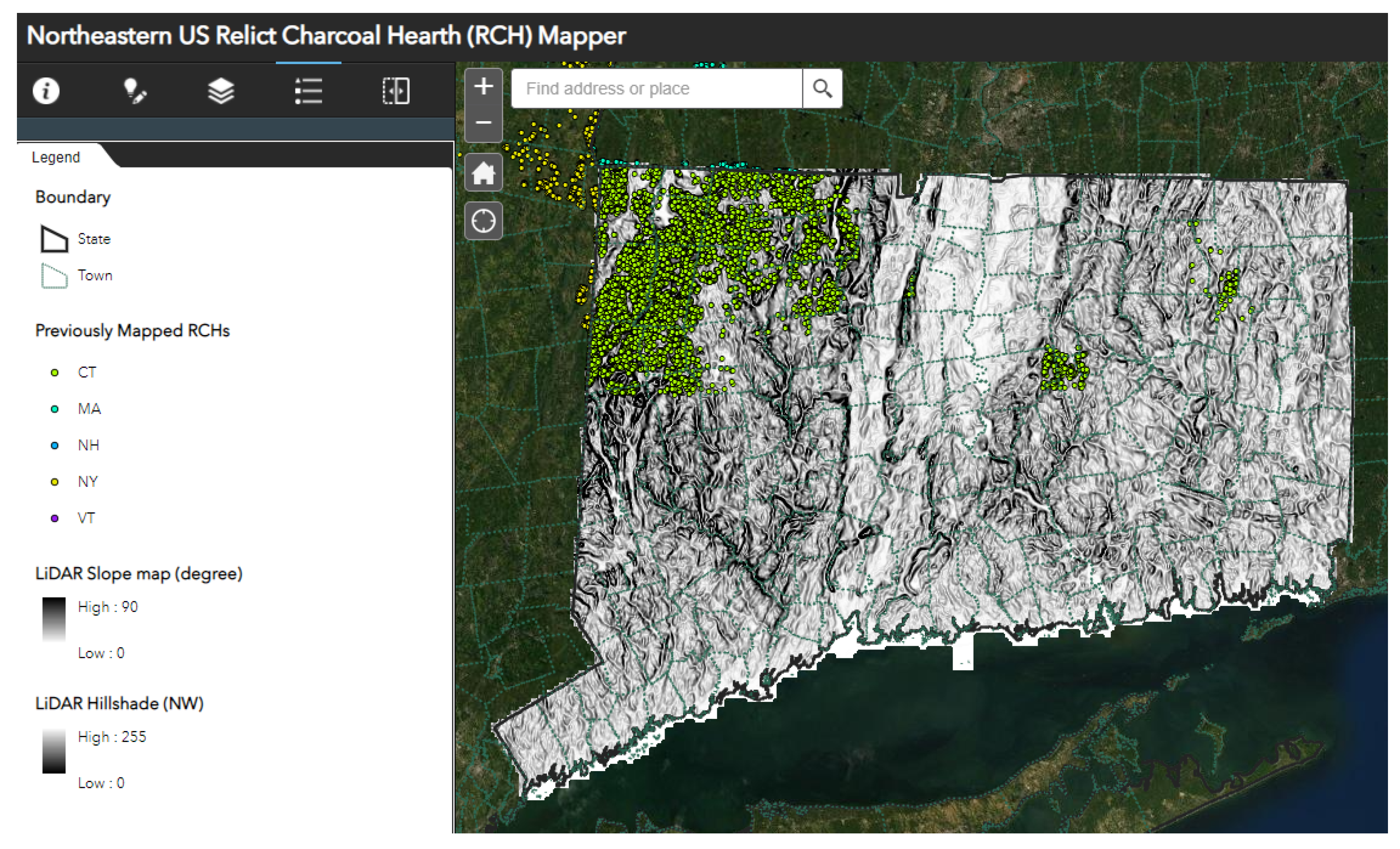
2.2.2. Reference Data

Reference data of RCH distribution is required since the Deep Convolutional Neural Networks (DCNNs) model used in this study is a supervised learning method. Previous studies in the region have used manually digitized RCHs based on 2011 Northwest LiDAR data [31] to examine various impacts including geomorphology [3] and forest cover [1]. Figure 3 shows the distribution of RCHs digitized by [1] and [3] published in an ArcGIS WebApp called ‘Northeastern US Relict Charcoal Hearth (RCH) Mapper’. Reference data that are used in this study could have missing RCHs depending on digitizers’ interpretations; manual digitization and user error (e.g., over- or under- mapping tendency depending on users) in this region is discussed in depth in [38]. In addition to this, the quality of LiDAR acquired in 2011 (used for RCH digitization in previous studies) and 2016 (used for model training and prediction in this study) can vary due to slight differences in forest canopy at the time of acquisition and overall point density and point spacing [39].

2.3. Methodology

The workflow (Figure 4) for detecting RCHs includes the following five steps: (1) image preparation for the U-Net model (training and validation samples), (2) model training and validation, (3) model prediction for six test regions, (4) post-processing of model predictions, and (5) accuracy assessment.

2.3.1. Preparing Input Data for the U-Net Model

Table 2 shows the four input scenarios as follows: (1) slope only (single band), (2) VAT only (single band), (3) composition of slope and hillshade rasters (7 bands), and (4) adding VAT raster to scenario 3 (8 bands).
Compared to a multi-band image, using the single band slope raster and single band VAT raster is a computationally efficient method. However, using a multi-band raster can improve model performance by extracting various feature maps during training. Scenario 3 used multiple rasters composed of slope and hillshade rasters. Hillshade allows visualization of different aspects of morphological features based on sun-angle azimuth so that six different azimuth angles were utilized; 0°, 45°, 90°, 180°, 270°, and 315°. Scenario 4 consisted of rasters from scenario 2 (single band VAT raster) and scenario 3 (7-band rasters). Input images for each scenario were normalized between 0 to 1 to speed up the training process.
For reference data, the digitized RCH point feature class was buffered to include the circumference of the RCH given that an average diameter of an RCH is ~7–12 m. The buffer threshold was 8 m (diameter 16 m) because not all digitized RCH points are in the centroid of the feature (see Section 2.2.2 for information on user digitization error). The buffered polygon was then rasterized using ArcGIS Pro.
Once input training rasters and reference data were produced, both datasets were sliced into small image patches (256 pixels by 256 pixels) to avoid an out of memory issue which occurred when the entire training image was fed into the model. Next, a data augmentation technique was applied to increase the number of training images by random rotation (e.g., 90 degree rotation, vertical or horizontal flip). As a result, the total number of input patches was 13,110 and among them, 90% of patches were used for the training model and the remaining 10% of patches were used for validation during the training process to keep track of model performance.

2.3.2. U-Net Model Training

The U-Net model is a DCNNs semantic segmentation model. It was first proposed by [40] and it has been modified and widely applied in remote sensing image analysis [41,42,43,44,45]; examples include Sentinel-2 imagery and other high resolution aerial imagery. The architecture of U-Net consists of encoder-decoder branches (Figure 4). During encoder branches (down-sampling), input image tiles are passed through five convolutional blocks to extract feature maps. Each block is composed of two sets of 3 × 3 kernel size convolutional layers followed by a rectified linear unit (ReLU) as an activation function. With a given number of channel depths (here we used 32, 64, 128, 256, and 512 for each convolutional block), a number of feature maps were extracted through the convolutional layer. Then a 2 × 2 max pooling layer was adopted to halve input spatial size (i.e., length and width) to reduce computational burden and highlight important information in the extracted feature map.
Decoder branches (up-sampling) are composed of five transposed convolutional blocks which increase tensor size (16 × 16 pixels in the 5th convolutional block) to original input image (here, 256 × 256 pixels) after passing through all transposed convolutional blocks. Transposed convolutional blocks are similar to convolutional blocks except the max-pooling layer is replaced by a transpose layer to increase the resolution of the output feature map. In addition, feature maps generated with convolutional blocks are concatenated to the output of the transposed layer, which allows the model to learn to build more precise output. Regarding concatenation, the size of the input feature should be the same so that it is applied to a convolutional block 4 (conv 4)—transpose convolutional block 1 (tran 1), conv 3—tran 2, conv 2—tran 3, and conv 1—tran 4. After passing through the decoder branch, a 1 × 1 convolutional layer was implemented followed by sigmoid function to reduce the depth of output and segment output to a binary image (i.e., RCHs or background). The total number of trainable parameters was about 7.7 million. The code used in this study has been made available at: https://github.com/twin22jw/RCH-detection (accessed on 14 November 2020).
Once model training was initialized, the weight and bias of nodes connected with these trainable parameters were updated to minimize loss value (error) between model prediction and reference data. In particular, the model training process is based on end-to-end learning using backpropagation, which means model parameters are updated automatically based on a backpropagation. With this model architecture and training process, the U-Net model was implemented and modified to deal with an overfitting issue and GPU memory limitation. In order to avoid the overfitting issue, a batch normalization layer [46] and a dropout layer after ReLU activation function layer were added in the convolutional block. In addition, a batch size of 16 was used to train the model on an 8 Gigabyte RTX 2070. Table 3 shows specific hyperparameters used for model training in this study.

2.3.3. Model Prediction

Model prediction was conducted in two ways. Firstly, the model from the four input scenarios (S1: single slope raster, S2: single VAT raster, S3: 7 bands composited with slope and hillshade rasters, S4: S2 + S3) was tested in 6 test regions as described in Table 1. The model prediction result was a binary output raster, where a value of 1 refers to RCH-like pixels and a value of 0 is background (or non-RCH) pixels. The model was employed at a broader scale for five towns (i.e., administrative entity) in northwestern Connecticut (bolded town boundaries in Figure 2) to evaluate model performance over a broader region.

2.3.4. Post-Processing

Post-processing was conducted on the binary output raster to reduce noisy pixels and convert it into point shapefile to extract RCH locations. First, vectorization was used to convert RCH pixels in the output raster into polygons with ArcGIS Pro. In some cases, more than two polygons were created for the same RCH because of isolated pixels near the main RCH. To clear up these unnecessary polygons, noisy and fragmented polygons from the vectorization process were deleted based on an area threshold (less than 30 m2). The polygons were then converted into a point shapefile using the Feature to Point tool in ArcGIS Pro.

2.3.5. Accuracy Assessment

Recall, precision, and F1 scores were used for accuracy assessment in the analysis of test regions. Three evaluation metrics were calculated based on true positive, false negative, and false positive. True positive refers to an actual RCH that is predicted as an RCH by the model. False negative is an actual RCH that is not predicted as an RCH by the model. False positive is not an actual RCH but is predicted as one by the model.
Recall is the ratio of positives identified by the model to the actual number of true positives in the reference data (i.e., true positives plus false negatives identified by the model) and is measured by the following equation:
R e c a l l = t r u e   p o s i t i v e s   /   ( t r u e   p o s i t i v e s + f a l s e   n e g a t i v e s )
Precision, on the other hand, is the ratio of true positives compared to all positives identified by the model and is measured by the equation:
P r e c i s i o n = t r u e   p o s i t i v e s   /   ( t r u e   p o s i t i v e s + f a l s e   p o s i t i v e s )
To assess the overall model performance, the F1 score was used and calculated by the following equation:
F 1   s c o r e = 2 × ( ( r e c a l l   ×   p r e c i s i o n )   /   ( r e c a l l + p r e c i s i o n ) )

3. Results and Discussion

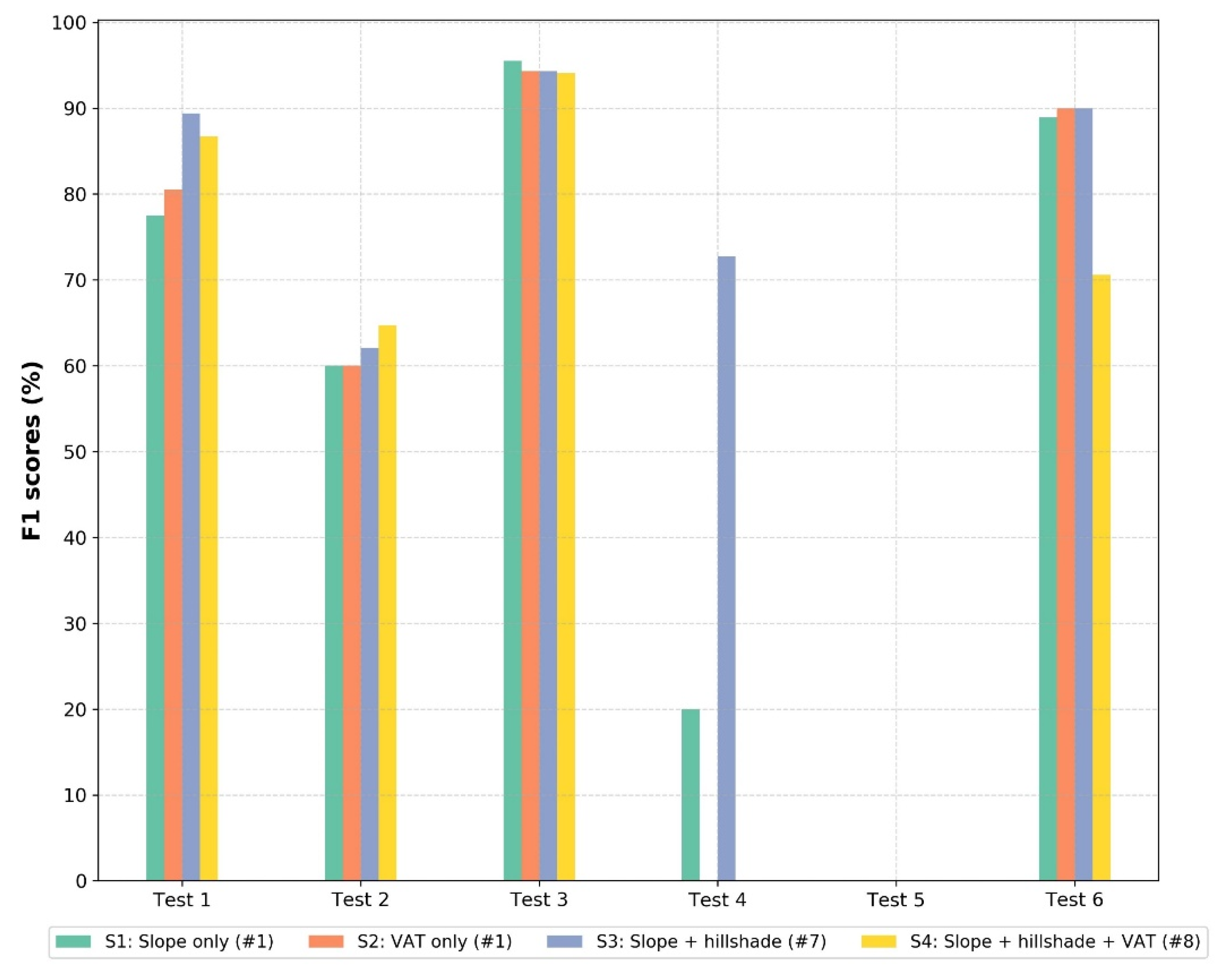
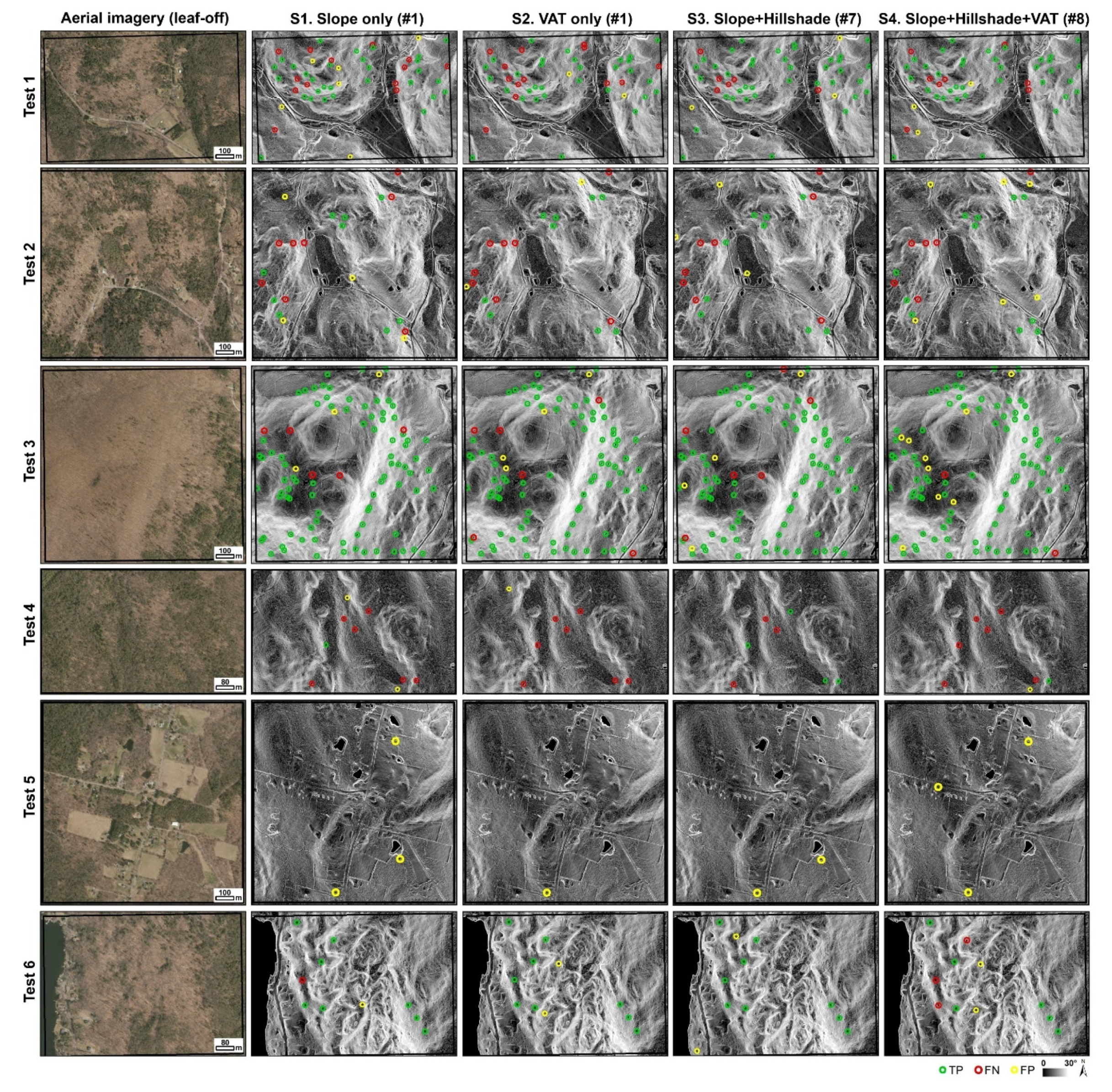
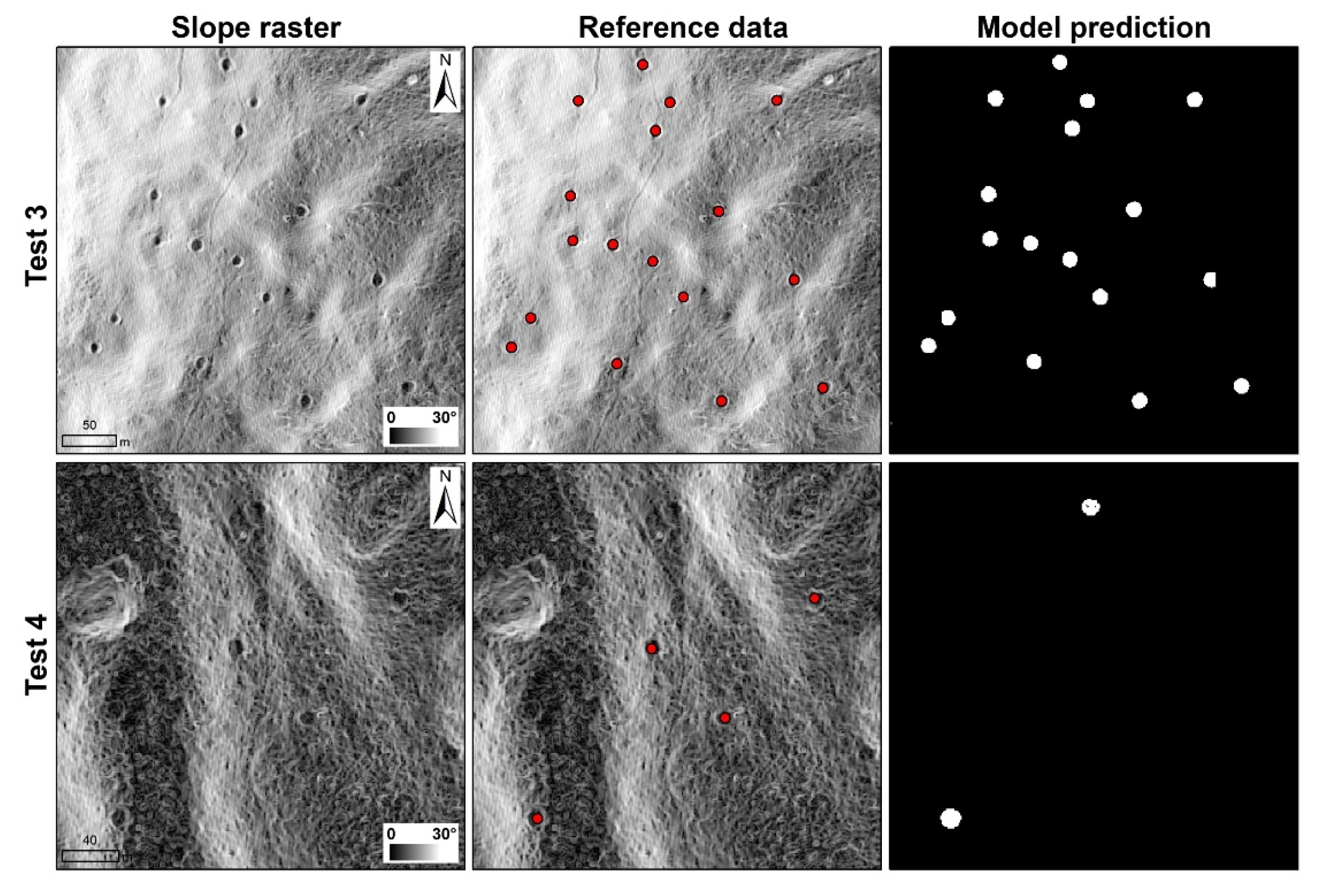
3.1. Results in the Six Test Regions

The accuracy assessment results of the U-Net model performance for the four input scenarios is summarized in Table 4 and Figure 5. The highest F1 score was 95.5% (S1) in test region 1 and the lowest F1 score was 0% (S2 and S4) in test region 4. Results were influenced by input scenario, nature of slope angle where RCHs are present in test regions, and landscape/land cover types. The highest F1 score for each input scenario was sensitive to the different qualities of each of the test regions. Overall, S3 performed well and has the highest F1 score in three of the test regions: region 1 (89.4%), 4 (72.7%), and 6 (90%) (Figure 5). Results also highlight that multi-raster scenarios (S3 or S4) can contribute to an improvement in model performance (see test regions 1, 2, 4, 6) and can be suitable to apply to study areas with diverse terrain conditions. A single raster can also have better performance in areas where there is a high concentration of RCHs in a high slope region.
The general morphological characteristics of RCHs in the study area (high slope edge and flat, round surface in otherwise-high slope area) makes them clearly visible in LiDAR raster derivatives (Figure 6). A previous study concluded that RCHs in high slope areas (e.g., >15 degrees) tend to be identified by the model relatively easily compared to those in low slope areas (e.g., <15 degrees) [21]. Model performance was good (F1 scores > 94%) in test region 3 where RCHs were high density and appeared on high slope areas (Figure 7). The poor model performance in test region 4 (F1 score < 20% with the exception of scenario 3) could be related to the fact that false negatives tend to occur in low slope areas, and these conditions are dominant in test region 4 (see Figure 7).
Modern land cover, particularly coniferous forest or developed areas, can also lead to false negatives or false positives. For example, the poor results in test region 4 could be related to LiDAR quality as well as the low slope terrain on which the RCHs appear (see Figure 7). The dominant land cover in test region 4 is coniferous forest (see Figure 6), which retains leaf cover year-round and can prevent laser pulses from reaching the ground surface at equivalent point densities to cleared areas [32]. Relatively low density point clouds in areas of coniferous forest can result in a rough texture in LiDAR derivatives due to the lack of points available for interpolation in these areas [4]. As a result, the precision of RCH morphology can suffer in visualizations of LiDAR raster derivatives. Our results show that using multiple hillshade rasters (S3) can supplement this limitation.

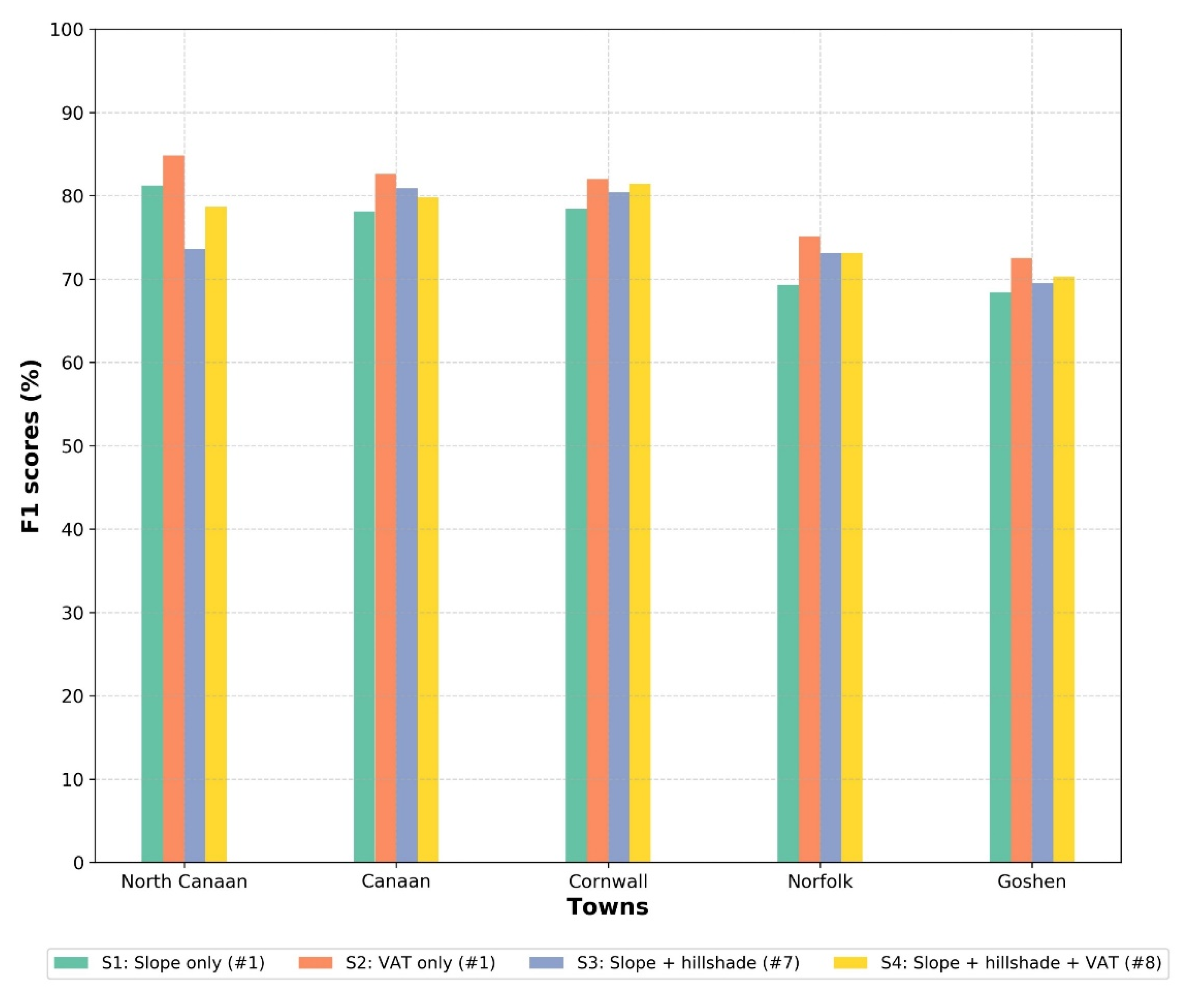
3.2. Results of Accuracy Assessment over Broad Region

Because the F1 score can be sensitive when true or false positive, or false negative samples are too small, we applied our model to five towns (North Canaan, Canaan, Cornwall, Norfolk, and Goshen) in the Salisbury Iron District to evaluate the overall model performance over a broad area (Figure 1). Previously, model performance was evaluated at smaller extents with a limited number of RCH samples. This accuracy assessment was conducted with the same post-processing described in Section 2.3.4 and Table 5 shows precision, recall, and F1 score results of the four input scenarios in the five study towns. Unlike the result in the six test regions, S2 performed the best in all five towns, with an F1 score ranging from 72.5% to 84.8% (Figure 8). This is partly due to the fact that the six test regions include RCH cases in various environments such as deciduous forest, coniferous forest, cleared fields, and developed areas. In the broader town areas, most RCHs are distributed in deciduous forest with smooth terrain along high slope regions and are well articulated in the VAT raster. Therefore, the single VAT raster has the advantage of avoiding a computational burden as well as achieving great performance to detect RCHs distributed in deciduous forest and smooth terrain with high slopes.
As briefly mentioned in Section 2.2.2, reference data may have error related to user or the quality of LiDAR data. This could affect accuracy assessment result since model performance was evaluated based on the reference. For example, Figure 7 showed a missing RCH in test region 4 (upper middle area) in reference data and it was regarded to as false positive. However, our model discovered new RCH site that is indeed RCHs and should be added to the regional datasets. Therefore, our model can contribute to find new RCH sites that were missed in the reference data (regional RCH datasets).

3.3. Model Performance and Landscapes

The accuracy assessment of the S2 model results in five towns was conducted in terms of land cover types such as deciduous forest, coniferous forest, and other types and slope angles with a threshold of 15° degrees (i.e., low slope vs. high slope). Table 6 shows the overview of accuracy assessment results, indicating model performance can be affected by land cover and slope angle conditions. Based on the F1 score, deciduous forest and regions with high slopes are favorable land cover types and slope conditions for the model (F1 score: 86.8%). As mentioned above, model results can be affected by the quality of LiDAR data (i.e., the density of the point cloud) because the input image is a derivative, and can also be affected by morphological characteristics of the RCH depending on the background slope conditions. For example, RCHs in regions with high slopes have more distinct morphological characteristics as an oval-shaped platform built deeply into the slope. This leads to a difference in slope between the middle and edge of the RCH, which provides a clearer delineation between minor slope differences whereas RCHs in low slope regions are more circular ramparts with slightly leveled platforms around the hearth [29]. RCHs in both deciduous and coniferous forest show high precision compared to recall score regardless of slope condition. However, the model shows an increase in false positives (low precision score) identifying RCHs in other landscapes such as developed, cleared fields, or agricultural land. Specifically, building foundations, wells, pools, or road and field edges are features that can confuse the model due to their morphological similarity to RCHs in LiDAR derivatives.
Figure 9 shows the distribution of true positives (TP), false negatives (FN), and false positives (FP) identified by the S2 model in different slope and land cover types. As described earlier, true positives are better discerned in deciduous forest along highly sloped regions or slightly sloped hills. Unlike true negatives (omission error) which often occur as RCHs clustered in deciduous forest, false positives occur as intermittent patterns across developed or other agricultural lands where one would not expect to find RCHs.

3.4. Comparison of Model Performance to Previous Research

Our model prediction results were compared to the results from other anthropogenic feature detection research using LiDAR-derived datasets and a DL approach [9,10,11,24]. However, it is difficult to simply compare in terms of F1 scores because target features and the spatial scale for model prediction are different. For example, model performance can depend on how morphological properties are distinctly visualized on LiDAR derivatives, which can also be dependent on LiDAR dataset quality and land cover conditions. In addition, a broad spatial scale for the model test area can increase omission and commission, resulting in a decrease of the F1 score [9]. Table 7 shows the overview of the results of previous research including remote sensing data, target feature, the spatial scale of test area, precision, recall, and F1 scores.
In terms of the DL method, object detection models (Faster R-CNN [11] and R-CNN [9]) and semantic segmentation models (ResNet [24] and U-Net) have been implemented. The accuracy of the model tends to decrease as spatial scale increases, as described in [9], and this is indeed supported by our results. However, over broader scales, the accuracy metrics range from a low score (e.g., below 50%) to a very high score (e.g., over 80%) [11], and compared to the results of previous studies, the results of our model show a high F1 score on average over regions of various sizes and extents.

3.5. Reconstruction of Historic Land Use Using Widespread RCH Mapping

Automated identification of anthropogenic features using deep convolutional neural networks provides an opportunity to reconstruct historic land use where land use has left traces identifiable on LiDAR data on at regional scales and at a fairly fine scale resolution [1]. The spatial distribution of anthropogenic features such as RCHs and stone walls in the northeastern U.S. can be used as a reliable proxy for estimating spatial extents of historic forest cover [1,49]. In this context, widespread mapping of RCHs using the DL approach proposed here will play a key role in understanding spatial aspects of historic land use dynamics in this region. For example, the distribution of RCHs in modern forested areas indicates the transition of land cover from forest to cleared land during periods of heavy iron production, and subsequent reforestation in the 20th century. Additionally, RCHs are indicative of other historical impacts to the landscape including geomorphological [3] and ecological [1]. A better understanding of their spatial distribution in the region allows for further quantification and study of historical impacts to the landscape that have persisted through the present.

4. Conclusions

This study found success in the application of a DL model (i.e., U-Net) to fully automate the extraction of anthropogenic features (RCHs) from high-resolution (i.e., 1m) LiDAR-based digital elevation models in New England. Our results provide a viable alternative to manual digitization of RCHs with promising accuracy even over broad extents and test regions. We implemented four input compositions of LiDAR derivatives: slope, hillshades, and VAT rasters to a U-Net model. In terms of input scenarios, the composition of slope and multiple directional hillshades tends to show the best performance over localized extents (e.g., less than 1.6 km2) of six test regions. At the town-level scale, the model was best able to detect RCHs using the single VAT raster. The model performed the best in areas of deciduous forest where slopes exceeded 15 degrees given that morphological characteristics of RCHs are well articulated in the LiDAR derivatives under these two conditions. Overall, the F1 scores of six test regions range from 62% to 94% (average: 82%) and those of five towns range from 73% to 86% (average: 80%). This is a significantly promising result compared to the previous studies that detect circular anthropogenic features.
With few exceptions, recent studies in the region have primarily used manual digitization methods to extract extant cultural landscape features, which can be time consuming. The results in this study present a reliable method of feature extraction and digitization at regional scales which will allow for reconstruction of regional historic forest cover, cultural resource management, and study of anthropogenic impacts at much broader scales than previously before. The model described in this study can be applied to detect possible RCH locations anywhere in the northeastern U.S. or other regions where high resolution LiDAR datasets are available.

Author Contributions

Conceptualization, J.W.S., E.A. and W.O.; methodology, J.W.S., E.A. and W.O.; validation, J.W.S., E.A. and W.O.; formal analysis, J.W.S., E.A. and W.O.; dataset development: J.W.S., E.A., W.O. and K.M.J., also see Acknowledgements; writing—original draft preparation, J.W.S., E.A., W.O.; writing—review and editing, J.W.S., E.A., W.O., K.M.J. and C.W.; funding acquisition, W.O. All authors have read and agreed to the published version of the manuscript.

Funding

This work was funded by National Science Foundation grant BCS-1654462 to W.O.

Institutional Review Board Statement

Not applicable.

Informed Consent Statement

Not applicable.

Data Availability Statement

The LiDAR DEM datasets used in this study are free and publicly available via CRCoG (see References). The multispectral orthography is publicly available via CRCoG (see References). The land cover map of 2015 is publicly available via CT CLEAR (see References). Digitized RCHs are available at the following ArcGIS Online maps: https://www.arcgis.com/apps/webappviewer/index.html?id=102f6831a12843878ea8081aec41029d (accessed on 14 November 2020).

Acknowledgments

In addition to the authors, the following individuals contributed to digitized datasets of relict charcoal hearths used in this study: Zac Raslan, Richard Ellsworth, and Ben Fellows.

Conflicts of Interest

The authors declare no conflict of interest.

References

  1. Johnson, K.M.; Ouimet, W.B. Reconstructing Historical Forest Cover and Land Use Dynamics in the Northeastern United States Using Geospatial Analysis and Airborne LiDAR. Ann. Am. Assoc. Geogr. 2021, 111, 1656–1678. [Google Scholar] [CrossRef]
  2. Straka, T.J. Historic Charcoal Production in the US and Forest Depletion: Development of Production Parameters. Adv. Hist. Stud. 2014, 3, 104–114. [Google Scholar] [CrossRef] [Green Version]
  3. Raab, T.; Hirsch, F.; Ouimet, W.; Johnson, K.M.; Dethier, D.; Raab, A. Architecture of relict charcoal hearths in northwestern Connecticut, USA. Geoarchaeology 2017, 32, 502–510. [Google Scholar] [CrossRef]
  4. Johnson, K.M.; Ouimet, W.B. An observational and theoretical framework for interpreting the landscape palimpsest through airborne LiDAR. Appl. Geogr. 2018, 91, 32–44. [Google Scholar] [CrossRef]
  5. Kemper, J. American Charcoal Making in the Era of the Cold-Blast Furnace; Electronic Document; U.S. Department of the Interior, National Park Service: Washington, DC, USA, 1941.
  6. Gordon, R.B. A Landscape Transformed: The Ironmaking District of Salisbury; Oxford University Press: New York, NY, USA, 2000. [Google Scholar]
  7. Witharana, C.; Ouimet, W.B.; Johnson, K.M. Using LiDAR and GEOBIA for automated extraction of eighteenth–late nineteenth century relict charcoal hearths in southern New England. GIScience Remote Sens. 2018, 55, 183–204. [Google Scholar] [CrossRef]
  8. Johnson, K.M.; Ouimet, W.B. Rediscovering the lost archaeological landscape of southern New England using airborne light detection and ranging (LiDAR). J. Archaeol. Sci. 2014, 43, 9–20. [Google Scholar] [CrossRef]
  9. Trier, Ø.D.; Reksten, J.H.; Løseth, K. Automated mapping of cultural heritage in Norway from airborne lidar data using faster R-CNN. Int. J. Appl. Earth Obs. Geoinf. 2021, 95, 102241. [Google Scholar] [CrossRef]
  10. Gallwey, J.; Eyre, M.; Tonkins, M.; Coggan, J. Bringing Lunar LiDAR Back Down to Earth: Mapping Our Industrial Heritage through Deep Transfer Learning. Remote Sens. 2019, 11, 1994. [Google Scholar] [CrossRef] [Green Version]
  11. Verschoof-van der Vaart, W.B.; Lambers, K. Learning to Look at LiDAR: The Use of R-CNN in the Automated Detection of Archaeological Objects in LiDAR Data from the Netherlands. J. Comput. Appl. Archaeol. 2019, 2, 31–40. [Google Scholar] [CrossRef] [Green Version]
  12. Carter, B.P.; Blackadar, J.H.; Conner, W.L.A. When Computers Dream of Charcoal: Using Deep Learning, Open Tools, and Open Data to Identify Relict Charcoal Hearths in and around State Game Lands in Pennsylvania. Adv. Archaeol. Pract. 2021, 1–15. [Google Scholar] [CrossRef]
  13. Chase, A.F.; Chase, D.Z.; Fisher, C.T.; Leisz, S.J.; Weishampel, J.F. Geospatial revolution and remote sensing LiDAR in mesoamerican archaeology. Proc. Natl. Acad. Sci. USA 2012, 109, 12916–12921. [Google Scholar] [CrossRef] [Green Version]
  14. Bennett, R.; Welham, K.; Hill, R.A.; Ford, A. A comparison of visualization techniques for models created from airborne laser scanned data. Archaeol. Prospect. 2012, 19, 41–48. [Google Scholar] [CrossRef]
  15. Howey, M.C.L.; Sullivan, F.B.; Tallant, J.; Kopple, R.V.; Palace, M.W. Detecting precontact anthropogenic microtopographic features in a forested landscape with lidar: A case study from the Upper Great Lakes Region, AD 1000-1600. PLoS ONE 2016, 11, e0162062. [Google Scholar] [CrossRef] [PubMed]
  16. Hesse, R. LiDAR-derived local relief models-a new tool for archaeological prospection. Archaeol. Prospect. 2010, 17, 67–72. [Google Scholar] [CrossRef]
  17. Štular, B.; Kokalj, Ž.; Oštir, K.; Nuninger, L. Visualization of lidar-derived relief models for detection of archaeological features. J. Archaeol. Sci. 2012, 39, 3354–3360. [Google Scholar] [CrossRef]
  18. Iriarte, J.; Robinson, M.; de Souza, J.; Damasceno, A.; da Silva, F.; Nakahara, F.; Ranzi, A.; Aragao, L. Geometry by Design: Contribution of Lidar to the Understanding of Settlement Patterns of the Mound Villages in SW Amazonia. J. Comput. Appl. Archaeol. 2020, 3, 151–169. [Google Scholar] [CrossRef]
  19. Doneus, M. Openness as visualization technique for interpretative mapping of airborne lidar derived digital terrain models. Remote Sens. 2013, 5, 6427–6442. [Google Scholar] [CrossRef] [Green Version]
  20. Evans, D.H.; Fletcher, R.J.; Pottier, C.; Chevance, J.B.; Soutif, D.; Tan, B.S.; Im, S.; Ea, D.; Tin, T.; Kim, S.; et al. Uncovering archaeological landscapes at Angkor using lidar. Proc. Natl. Acad. Sci. USA 2013, 110, 12595–12600. [Google Scholar] [CrossRef] [Green Version]
  21. Schneider, A.; Takla, M.; Nicolay, A.; Raab, A.; Raab, T. A template-matching approach combining morphometric variables for automated mapping of charcoal kiln sites. Archaeol. Prospect. 2015, 22, 45–62. [Google Scholar] [CrossRef]
  22. Orengo, H.A.; Conesa, F.C.; Garcia-Molsosa, A.; Lobo, A.; Green, A.S.; Madella, M.; Petrie, C.A. Automated detection of archaeological mounds using machine-learning classification of multisensor and multitemporal satellite data. Proc. Natl. Acad. Sci. USA 2020, 117, 18240–18250. [Google Scholar] [CrossRef] [PubMed]
  23. Guyot, A.; Hubert-Moy, L.; Lorho, T. Detecting Neolithic burial mounds from LiDAR-derived elevation data using a multi-scale approach and machine learning techniques. Remote Sens. 2018, 10, 225. [Google Scholar] [CrossRef] [Green Version]
  24. Trier, Ø.D.; Cowley, D.C.; Waldeland, A.U. Using deep neural networks on airborne laser scanning data: Results from a case study of semi-automatic mapping of archaeological topography on Arran, Scotland. Archaeol. Prospect. 2019, 26, 165–175. [Google Scholar] [CrossRef]
  25. Guyot, A.; Lennon, M.; Hubert-moy, L. Combined Detection and Segmentation of Archeological Structures from LiDAR Data Using a Deep Learning Approach. J. Comput. Appl. Archaeol. 2021, 4, 1–19. [Google Scholar] [CrossRef]
  26. Davis, D.S.; Lundin, J. Locating Charcoal Production Sites in Sweden Using LiDAR, Hydrological Algorithms, and Deep Learning. Remote Sens. 2021, 13, 3680. [Google Scholar] [CrossRef]
  27. Gordon, R.B.; Raber, M. Industrial Heritage in Northwest Connecticut: A Guide to History and Archaeology; Connecticut Academy of Arts and Sciences: New Haven, CT, USA, 2000. [Google Scholar]
  28. Foster, D.R.; Donahue, B.; Kittredge, D.; Motzkin, G.; Hall, B.; Turner, B.; Chilton, E. New England’s Forest Landscape. Agrar. Landsc. Transit. 2008, 44–88. [Google Scholar]
  29. Anderson, E. Mapping Relict Charcoal Hearths in the Northeast US Using Deep Learning Convolutional Neural Networks and LIDAR Data; University of Connecticut: Storrs, CT, USA, 2019. [Google Scholar]
  30. Capitol Region Council of Governments (CRCoG). Connecticut Statewide LiDAR 2016 Bare Earth DEM. Available online: http://www.cteco.uconn.edu/metadata/dep/document/lidarDEM_2016_fgdc_plus.htm (accessed on 14 November 2021).
  31. Connecticut Environmental Conditions Online NRCS Northwest LiDAR 2011 Metadata. Available online: https://cteco.uconn.edu/data/lidar/docs/NWLidar/FGDC_CONNECTICUT_BARE_EARTH_LAS.xml (accessed on 14 November 2020).
  32. Doneus, M.; Briese, C.; Fera, M.; Janner, M. Archaeological prospection of forested areas using full-waveform airborne laser scanning. J. Archaeol. Sci. 2008, 35, 882–893. [Google Scholar] [CrossRef]
  33. Pfeifer, N.; Gorte, B.; Oude Elberink, S. Influences of vegetation on laser altimetry—Analysis and correction approaches. In Proceedings of the Natscan, Laser-Scanners for Forest and Landscape Assessment, Freiburg, Germany, 3–6 October 2004; Volume 36, pp. 283–287. [Google Scholar]
  34. Connecticut Environmental Conditions Online (CT ECO). Connecticut Statewide LiDAR 2016 Bare Earth DEM. Available online: https://cteco.uconn.edu/data/lidar/index.htm (accessed on 14 November 2020).
  35. Verbovšek, T.; Popit, T.; Kokalj, Ž. VAT method for visualization of mass movement features: An alternative to hillshaded DEM. Remote Sens. 2019, 11, 2946. [Google Scholar] [CrossRef]
  36. Kokalj, Ž.; Somrak, M. Why not a single image? Combining visualizations to facilitate fieldwork and on-screen mapping. Remote Sens. 2019, 11, 747. [Google Scholar] [CrossRef] [Green Version]
  37. Zakšek, K.; Oštir, K.; Kokalj, Ž. Sky-view factor as a relief visualization technique. Remote Sens. 2011, 3, 398–415. [Google Scholar] [CrossRef] [Green Version]
  38. Leonard, J.; Ouimet, W.B.; Dow, S. Evaluating User Interpretation and Error associated with Digitizing Stone Walls using airborne LiDAR. Geol. Soc. Am. Abstr. Programs 2021, 53. [Google Scholar] [CrossRef]
  39. Johnson, K.M.; Ives, T.H.; Ouimet, W.B.; Sportman, S.P. High-resolution airborne Light Detection and Ranging data, ethics and archaeology: Considerations from the northeastern United States. Archaeol. Prospect. 2021, 28, 293–303. [Google Scholar] [CrossRef]
  40. Ronneberger, O.; Fischer, P.; Brox, T. U-net: Convolutional networks for biomedical image segmentation. Med. Image Comput. Comput. Interv. 2015, 9351, 234–241. [Google Scholar] [CrossRef] [Green Version]
  41. Mboga, N.; Grippa, T.; Georganos, S.; Vanhuysse, S.; Smets, B.; Dewitte, O.; Wolff, E.; Lennert, M. Fully convolutional networks for land cover classification from historical panchromatic aerial photographs. ISPRS J. Photogramm. Remote Sens. 2020, 167, 385–395. [Google Scholar] [CrossRef]
  42. Yan, S.; Xu, L.; Yu, G.; Yang, L.; Yun, W.; Zhu, D.; Ye, S.; Yao, X. Glacier classification from Sentinel-2 imagery using spatial-spectral attention convolutional model. Int. J. Appl. Earth Obs. Geoinf. 2021, 102, 102445. [Google Scholar] [CrossRef]
  43. Peng, D.; Zhang, Y.; Guan, H. End-to-end change detection for high resolution satellite images using improved UNet++. Remote Sens. 2019, 11, 1382. [Google Scholar] [CrossRef] [Green Version]
  44. Waldner, F.; Diakogiannis, F.I. Deep learning on edge: Extracting field boundaries from satellite images with a convolutional neural network. Remote Sens. Environ. 2020, 245, 111741. [Google Scholar] [CrossRef]
  45. Stoian, A.; Poulain, V.; Inglada, J.; Poughon, V.; Derksen, D. Land cover maps production with high resolution satellite image time series and convolutional neural networks: Adaptations and limits for operational systems. Remote Sens. 2019, 11, 1986. [Google Scholar] [CrossRef] [Green Version]
  46. Ioffe, S.; Szegedy, C. Batch normalization: Accelerating deep network training by reducing internal covariate shift. In Proceedings of the 32nd International Conference on Machine Learning, ICML 2015, Lille, France, 6–11 July 2015; Volume 1, pp. 448–456. [Google Scholar]
  47. Capitol Region Council of Governments (CRCoG). 2016 Aerial Imagery. Available online: http://cteco.uconn.edu/data/flight2016/index.htm (accessed on 14 November 2020).
  48. Center for Land Use Education & Research (CT CLEAR). 2015 Connecticut Land Cover. Available online: https://clear.uconn.edu/projects/landscape/download.htm#top (accessed on 14 November 2020).
  49. Johnson, K.M.; Ouimet, W.B.; Dow, S.; Haverfield, C. Estimating Historically Cleared and Forested Land in Massachusetts, USA, Using Airborne LiDAR and Archival Records. Remote Sens. 2021, 13, 4318. [Google Scholar] [CrossRef]
Figure 1. Overview of study region and towns in Connecticut, United States. The background map depicts RCH presence or absence and RCH density (RCH count/km2) [29].
Remotesensing 13 04630 g001
Figure 2. Visualization of RCHs in three different rasters derived from a LiDAR DEM. (A) slope, (B) VAT (Visualization for Archaeological Topography), (C) hillshade; Note that (1) and (2) indicates an example cross section (a,b) through a RCH showing the elevation and slope profiles, respectively.
Remotesensing 13 04630 g002
Figure 3. Manually digitized RCHs map published in Northeastern US relict charcoal hearth mapper. (https://connecticut.maps.arcgis.com/apps/webappviewer/index.html?id=102f6831a12843878ea8081aec41029d) (accessed on 14 November 2020).
Remotesensing 13 04630 g003
Figure 4. The workflow of automated RCH detection using U-Net.
Remotesensing 13 04630 g004
Figure 5. F1 score results for input scenarios by six test regions. (input scenarios—S1: single slope raster, S2: single VAT raster, S3: 7 bands composition with slope and hillshades rasters, S4: 8 bands composition with slope, hillshades, and VAT rasters; # refers to the number of rasters for input image).
Remotesensing 13 04630 g005
Figure 6. Leaf-off aerial image and model prediction results for test regions 1–6. High resolution aerial images (2016) are provided by [47]. Note that # refers to the number of rasters for the input image. The background image for model prediction results is a slope raster (color ramp: black (low slope) to white (high slope). TP = true positive, FN = false negative, FP = false positive.
Remotesensing 13 04630 g006
Figure 7. The comparison of model prediction results between a subset of test region 3 (RCHs on high slopes in deciduous forest) and 4 (RCHs on low slopes in coniferous forest). Model prediction results are from input scenario 1 (single slope raster).
Remotesensing 13 04630 g007
Figure 8. F1 score results for five towns (North Canaan, Canaan, Cornwall, Norfolk, and Goshen) in northwestern Connecticut. For Cornwall, accuracy was calculated without a training region. # refers to the number of rasters for input image.
Remotesensing 13 04630 g008
Figure 9. Slope map (generated from 1m LiDAR DEM) (A), land cover map (2015, 30 m resolution, provided by CT CLEAR) [48] (B), and S2 model prediction results for five towns (North Canaan, Canaan, Cornwall, Norfolk, and Goshen). RCHs in training site 1 were excluded during the accuracy assessment (C).
Remotesensing 13 04630 g009
Table 1. Size, landscape type, and RCH count in the test regions.
RegionArea (km2)Landscape TypeRCH Count
Test 10.94>15° slopes with developed regions (e.g., sparse residential area) and stream/river bed running through the area44
Test 21.59Developed region interspersed with >15° slopes17
Test 31.17>15° slopes with deciduous landscape89
Test 40.53<15° slopes with coniferous landscape7
Test 51.13Smooth terrain and cleared field with no RCHs0
Test 60.35>15° slopes with very rough terrain9
Table 2. Description of four input scenarios used in this study.
Input ScenariosDescription# of Rasters
Scenario 1 (S1)Slope1
Scenario 2 (S2)VAT1
Scenario 3 (S3)Slope and hillshades (azimuth angle: 0, 45, 90, 180, 270, 315 deg.)7
Scenario 4 (S4)Slope, hillshades (azimuth angle: 0, 45, 90, 180, 270, 315 deg.), and VAT8
Table 3. Hyperparameters for model training.
HyperparameterValue/Type
Batch size16
OptimizerAdam
Learning rateInitially starting from 0.001
Loss functionBinary Cross Entropy
EpochsUp to 30 (used early stopping callback)
Table 4. Accuracy assessment results of six test regions. Bold text represents the highest F1 score in each test region.
RegionInput ScenarioTrue PositivesFalse PositivesFalse NegativesPrecisionRecallF1 Score
Test 1S13161386.1%70.5%77.5%
S23121393.9%70.5%80.5%
S3383692.7%86.4%89.4%
S4363892.3%81.8%86.7%
Test 2S194869.2%52.9%60.0%
S292881.8%52.9%64.3%
S393875.0%52.9%62.1%
S4116664.7%64.7%64.7%
Test 3S1843596.6%94.4%95.5%
S2834695.4%93.3%94.3%
S3834695.4%93.3%94.3%
S4879290.6%97.8%94.1%
Test 4S112633.3%14.3%20.0%
S20170.0%0.0%0.0%
S3403100.0%57.1%72.7%
S40260.0%0.0%0.0%
Test 5S10300.0%N/AN/A
S20100.0%N/AN/A
S30200.0%N/AN/A
S40300.0%N/AN/A
Test 6S181188.9%88.9%88.9%
S292081.8%100.0%90.0%
S392081.8%100.0%90.0%
S462375.0%66.7%70.6%
Table 5. The results for the entire test region after post-processing. For Cornwall Town, accuracy was calculated without including train region. Bold text represents the highest F1 score in each town.
TownInput ScenarioTrue PositivesFalse PositivesFalse NegativesPrecisionRecallF1 Score
North CanaanS1235416885.14%77.56%81.2%
S2243285489.67%81.82%85.6%
S3223817973.36%73.84%73.6%
S4234606779.59%77.74%78.7%
CanaanS1175238959681.83%74.62%78.1%
S2195028753687.17%78.44%82.6%
S3187627161387.38%75.37%80.9%
S4187634061084.66%75.46%79.8%
CornwallS1210750865180.57%76.40%78.4%
S2228046653283.03%81.08%82.0%
S3223749759581.82%78.99%80.4%
S4228652652081.29%81.47%81.4%
NorfolkS1110551546468.21%70.43%69.3%
S2123535246677.82%72.60%75.1%
S3120638250575.94%70.49%73.1%
S4120238949775.55%70.75%73.1%
GoshenS153028120965.35%71.72%68.4%
S253717223675.74%69.47%72.5%
S355024923368.84%70.24%69.5%
S454723922369.59%71.04%70.3%
Table 6. Accuracy assessment results (true positive, false positive, false negative, precision, recall, and F1 scores) of the S2 model in five towns in terms of RCH condition (i.e., land cover type, slope degrees, and their combination). Bold text represents the highest F1 score in each landscape condition category.
Landscape ConditionTrue PositiveFalse PositiveFalse NegativePrecisionRecallF1 Score
Land coverDeciduous5013775126786.6%79.8%83.1%
Conifer113340651173.6%68.9%71.2%
Other991244644.4%68.3%53.8%
SlopeHigh (>15°)129318829087.3%81.7%84.4%
Low (>15°)49521117153481.6%76.3%78.9%
Land cover & slopeDeciduous & high slope106111520990.2%83.5%86.8%
Deciduous & low slope3952660105885.7%78.9%82.1%
Conifer & high slope215597478.5%74.4%76.4%
Conifer & low slope91834743772.6%67.7%70.1%
Other & high slope1714754.8%70.8%61.8%
Other & low slope821103942.7%67.8%52.4%
Table 7. Summary of the results (precision, recall, F1 score) of other studies that detecting anthropogenic features using DL.
AuthorRS DataDL MethodTarget Feature
(Diameter)
Spatial Scale (km2)Precision (%)Recall (%)F1 Score (%)
[10]LiDAR SLRM,
PO, NO
CNN (transfer learning)historic mining pits
(2~3 m)
1818081
0.2928387
[11]LiDAR SLRMFaster R-CNNbarrows10.9536–90
(avg.: 64)
62–81
(avg.: 73)
46–79
(avg.:67)
Celtic fields10.9526–71
(avg.: 46)
19–97
(avg.: 60)
29–68
(avg.: 43)
[24]LiDAR SLRMResNetroundhouse
(8~15 m)
432467356
small cairn
(~10 m)
432182019
shieling hut
(~20 m)
432122617
[9]LiDAR HS
and LRM
R-CNNgrave mounds
(~77 m)
16.58847076
pitfall traps
(4~7 m)
16.58868083
charcoal kilns
(10~20 m)
16.58966880
grave mounds
(~77 m)
67381421
charcoal kilns
(10~20 m)
937629073
Our studyLiDAR SP, HS, and VATU-Netcharcoal hearth
(7–12 m)
<1.5–49375–10053–10062–94
(avg.: 82)
76–9070–8273–86
(avg.: 80)
PO: Positive Openness; NO: Negative Openness, SLRM: simplified local relief model, HS: Hillshade, SP: Slope, VAT: Visualization for archaeological topography tool, avg.: average. Our result for small extent area (i.e., less than 1.5 km2) is based on S3 model and that for large extent area (i.e., 493 km2) is based on S2 model result.
Publisher’s Note: MDPI stays neutral with regard to jurisdictional claims in published maps and institutional affiliations.

