
High-Resolution Polar Low Winds Obtained from Unsupervised SAR Wind Retrieval


1
Department of Physics and Technology, UIT The Arctic University of Norway, 9037 Tromsø, Norway
2
Norwegian Meteorological Institute, 9293 Tromsø, Norway
3
NORCE Norwegian Research Center AS, 9294 Tromsø, Norway
*
Author to whom correspondence should be addressed.
Remote Sens. 2021, 13(22), 4655; https://0-doi-org.brum.beds.ac.uk/10.3390/rs13224655
Submission received: 18 October 2021
/
Revised: 13 November 2021
/
Accepted: 16 November 2021
/
Published: 18 November 2021
(This article belongs to the Special Issue High Winds and High Seas)
Abstract
:High-resolution sea surface observations by spaceborne synthetic aperture radar (SAR) instruments are sorely neglected resources for meteorological applications in polar regions. Such radar observations provide information about wind speed and direction based on wind-induced roughness of the sea surface. The increasing coverage of SAR observations in polar regions calls for the development of SAR-specific applications that make use of the full information content of this valuable resource. Here we provide examples of the potential of SAR observations to provide details of the complex, mesoscale wind structure during polar low events, and examine the performance of two current wind retrieval methods. Furthermore, we suggest a new approach towards accurate wind vector retrieval of complex wind fields from SAR observations that does not require a priori wind direction input that the most common retrieval methods are dependent on. This approach has the potential to be particularly beneficial for numerical forecasting of weather systems with strong wind gradients, such as polar lows.
1. Introduction
Backscatter images from spaceborne synthetic aperture radars (SARs) show sea surface conditions in great detail. In the absence of oil slicks or strong surface currents, the radar backscatter from the surface of the sea is mainly controlled by wind-induced ripples on the scale of the radar wavelength. The sub-kilometre details visible in SAR images appear predestined for the study of meteorological phenomena of the mesoscale, (1 km)–(100 km). Wind-retrieval methods for SARs aim to extract information about surface wind speed and direction from SAR backscatter images. The accurate and reliable high-resolution retrieval of sea surface wind fields from SAR observations is a necessity for subsequent applications such as assimilation into mesoscale numerical weather models, for nowcasting or for model validation of complex mesoscale wind phenomena, such as polar lows. Here, we demonstrate deficiencies of current methods in retrieving mesoscale wind fields and propose a way forward towards exhausting the wind information content of dual polarisation SAR images without using external wind direction information.
Geophysical model functions (GMFs) that relate wind speed and direction to the co-polarised backscatter of C-band microwave radiation from the sea surface were originally developed from the collocation of scatterometer observations and buoy wind observations or the surface wind field from numerical weather prediction (NWP) models. (Co-polarised means that the radar transmits and receives radiation in the same polarisation plane. Henceforth, the abbreviation copol is used). Scatterometers that employ several antennae can invert such GMFs to arrive at a surface wind field with an 180° ambiguity. The SAR observation principle allows for a much higher resolution than scatterometers can achieve. However, only a single antenna is possible for SAR. Therefore, the GMF inversion is underdetermined. This has been generally circumvented by providing wind direction as a priori information in what can be regarded as classical SAR wind retrieval algorithms. Sources of a priori wind direction are, for instance, provided from in-situ buoy wind measurements, linear features in the SAR image or, most commonly applied, numerical weather prediction models. From the combination of backscatter measurement and a priori wind direction, the most likely wind vector is determined by minimising a least-squares cost function (see Section 2.4).
The copol signal, which is commonly used in combination with a priori wind direction, becomes increasingly saturated for high wind speed ( 20 m s−1), meaning that increasing wind speed does not lead to a proportional increase of backscatter intensity e.g., [1,2,3,4]. Wind retrieval by inversion of a copol GMF therefore becomes less accurate for strong wind, because of signal saturation and insufficient tuning of GMFs for high wind speeds. Due to signal saturation, the classical copol wind retrieval is susceptible to large errors caused by the use of a wrong a priori wind direction during the retrieval. For crosspol backscatter, no such saturation has been reported, even in above hurricane-strength winds [5,6].
In contrast to the copol signal, the cross-polarised backscatter increases linearly with wind speed [6] and is virtually independent of wind direction (see Figure 1a). (Cross-polarised means that radiation is received in a 90° different polarisation plane than it is transmitted by the radar. Hereafter, the abbreviation crosspol is used). Hence, with regard to strong wind, the crosspol channel has an advantage over copol, but does not hold any information on wind direction. A major drawback with wind speed retrievals from crosspol backscatter is that, for low wind speed, the signal is weak and therefore becomes inseparable from instrument noise. A wind-retrieval approach that combines copol and crosspol backscatter with a priori wind direction has shown more realistic wind speed distribution in studies of hurricane winds [7,8]. In effect, the combined wind retrieval makes use of the copol channel for low to moderate winds and the crosspol channel for high wind speeds. This improves the wind speed retrieval which, however, still relies on a priori wind direction.
Most endeavours to extract wind direction information from SAR images have focused on linear features caused by organised roll vortices in the atmospheric boundary layer that are aligned with the wind direction e.g., [9]. Linear features are, however, not always present, can originate from other sources than roll vortices, and may not be exactly aligned with the surface wind field [6,10]. Independently of the presence of linear features from roll vortices, the Doppler frequency shift of the backscatter signal yields wind direction information relative to the radar look direction. The Doppler Centroid Anomaly (DCA) has been added to the classical probabilistic copol wind retrieval [11] to improve the retrieved wind direction in complex meteorological situations.
Ironically, small-scale complex meteorological situations, such as polar lows, which are well captured by high-resolution SAR observations are situations when current wind retrieval techniques perform poorly. Polar lows are intense, maritime, mesoscale cyclones, which develop rapidly in cold air masses that advance over large bodies of relatively warm water [12]. They typically have a lifetime of (1 day) and a horizontal extent of (100 km). Polar lows are often associated with heavy snowfall and strong winds. Due to their rapid development and small extent, they pose a challenge for NWP models. Even high-resolution weather models, such as AROME-Arctic, which are able to simulate realistic polar lows, suffer from a lack of observations on the scales of polar lows that can enter assimilation [13]. Polar lows occur at high latitudes where SAR coverage is ample. This opens up the possibility that high-quality wind retrieval becomes a valuable asset for assimilation into numerical models and thereby potentially improves forecasts of polar lows.
![Remotesensing 13 04655 g001]()
Figure 1.
Geophysical model functions that relate wind speed (m s−1) and direction (° relative to radar) to a measured quantity. The GMFs are shown for a 30° incidence angle and the black lines indicate isolines of constant backscatter intensity (dB) and Doppler shift (Hz). The 0° wind direction is wind blowing towards the radar and angles increase clockwise. (a) Shows the crosspol GMF, MS1A [7]; (b) the copol GMF, CMODH [14]; and (c) a GMF for the Doppler centroid anomaly, [15].

2. Materials and Methods
2.1. Sentinel-1 Synthetic Aperture Radar
The C-band SAR data used here were collected by the SAR instruments aboard the two identical polar orbiting satellites (Sentinel-1 A/B) of the European Space Agency’s Sentinel-1 mission [16]. The two satellites fly in the same orbital plane with a 180° phase difference. This constellation can potentially image most of the European Arctic in all weather conditions, twice daily on a descending (southward) morning pass, and an ascending (northward) evening pass. In practice, this potential is not realised due to the alternation between different observation modes over land and sea surfaces, the interferometric wide swath mode (IW) and the extra wide swath mode (EW), respectively. The mode transition results in missing data in transition zones. For ocean applications in the European Arctic, the ascending evening pass is especially affected by such data losses. For this study, dual polarisation data in EW mode are used. Dual polarisation here means that, for signal transmission, the oscillations of the electric field vector are confined to the horizontal plane (in antenna coordinates); however, both horizontally and vertically, polarised backscatter is received. The 410 km wide EW-swath images used here consist of five sub-swaths and have approximately 93 × 87 m resolution in range (normal to flight direction) and azimuth (parallel to flight direction) direction, respectively. The dual polarisation observation mode results in two data sets for each image, one for the horizontally polarised transmitted and received signal (HH) known as the copol signal, and the other channel for the horizontally polarised transmission and vertically polarised backscatter (HV) referred to as crosspol signal.
2.2. AROME-Arctic Numerical Weather Forecasting Model
The AROME-Arctic model is a high-resolution regional forecasting system that is adapted for the European Arctic [17]. The horizontal grid spacing of AROME-Arctic is 2.5 km and its vertical structure is made up of 65 hybrid pressure and terrain-following levels. The dynamical core solves the non-hydrostatic fully elastic Euler Equations [18]. The model is initialised based on a 3D variational data assimilation system and boundary conditions come from the ECMWF HRES global forecasting system. 66 h forecasts are produced four times a day (0300, 0600, 1200, 1800 utc) with short-term 3 h forecasts in between. With a resolution that is high enough to partly resolve convection, AROME-Arctic is well suited to study mesoscale phenomena such as polar lows [19]. AROME-Arctic is very similar to the main Scandinavian operational model AROME-MetCoOp and further details about both models are described in [17,20] and references therein. The high-resolution of AROME-Arctic allows it to realistically model mesoscale meteorological phenomena, such as downslope windstorms or polar lows. However, due to the limited availability of observations, high-resolution models lack forcing from assimilated information at the relevant scales.
2.3. In Situ Observations
Satellite observations and model results of a polar low event are compared with in situ wind observations from land-based surface weather stations. For the comparison, only coastal stations that had valid SAR observations within a 3 km radius were used. All available stations that fulfil this requirement during the example polar low event are shown in Figure 2b. The comparison of wind observations from land-based observation sites with wind that was retrieved from radar backscatter of the sea surface contains caveats: even within a 3 km radius, orographic steering and sheltering of the wind, as well as the difference in surface friction, could result in large differences between winds that are observed in close proximity on land and at sea. In the absence of better alternatives, observations from land stations are used as an ancillary source of information. It is, however, emphasised that these in situ observations do not represent a ground truth.
2.4. Wind Retrieval Techniques
In general, wind retrieval methods are based on the inversion of empirical GMFs that relate to a geophysical quantity (here, the surface wind), to an observed quantity, such as radar backscatter, or the Doppler centroid anomaly. The three GMFs that were applied here—MS1A for crosspol backscatter [7], CMODH for copol backscatter [21], and a GMF for the Doppler centroid anomaly, [15]—are shown in Figure 1a–c.
The crosspol GMF that is used here, MS1A, does not depend on wind direction (Figure 1a). Therefore the relationship between wind speed and backscatter is easily inverted and a wind speed retrieval with MS1A is computationally economical. The most decisive disadvantages of the wind speed retrieval by inversion of MS1A are that no information about the wind direction is gained and that the low signal-to-noise ratio of crosspol observations exerts a lower limit on wind speed retrieval.
The copol GMF CMODH relates wind speed and direction to the horizontally polarised backscatter from SAR. CMODH is the latest SAR-specific GMF in a row of C-band model functions that initially were developed for the use with scatterometer observations. The difference between CMODH and other CMOD GMFs is that CMODH is developed for horizontally polarised SAR backscatter. At high latitudes, HH polarisation is the common observation mode instead of VV because of advantages for sea ice applications. By using CMODH the translation from HH to VV backscatter using a polarisation ratio model can be avoided, thus eliminating a potential source of error. Since the copol backscatter depends on both wind speed and direction (Figure 1b), the inversion problem is underdetermined. This dilemma of the classical wind retrieval is usually overcome by providing auxiliary information about the wind direction from a numerical weather prediction model or from elsewhere. In addition to supplementary wind direction information, a probabilistic solution for the wind vector is derived by minimising a cost function, such as
where is the a priori wind vector that normally comes from a NWP model, is the simulated radar backscatter using a GMF of the CMOD type and is the measured copol signal. and are the Gaussian error standard deviations that are most commonly assumed to be constants. The retrieved wind vector is where has its minimum. Depending on the size of the errors in the denominators, the a priori term constrains the wind retrieval to the model wind vector. Refer to [22] for a detailed description of the classical probabilistic approach that has been applied to, and evaluated for SAR observations derived from instruments aboard a variety of satellite missions, e.g., [23,24]. A flaw of this method is that an incorrect model wind direction as input leads to a incorrect and physically inconsistent wind field. This is a result of using constant in the a priori term, which effectively ignores the possibility of the model error being large.
The Doppler (DC) frequency shift is the centroid of the azimuth spectra, and consists of a geometric term (orbit/altitude/antenna) and a geophysical term arising from surface motion (wind/wave/current) [25]. The geophysical term is often called the Doppler centroid anomaly (DCA). Here, the DCA estimation is performed following the algorithm of ESA OCN L2 product [26,27]. The DCA frequency contains an artefact velocity caused by the wave motion and the imaging process, and a genuine velocity from the Lagrangian mean surface current. The artefact velocity is highly correlated with the local wind speed component in the line-of-sight direction [15,28] (Figure 1c), and is often much larger than the Lagrangian mean surface current signal. It has been demonstrated that the classical copol wind retrieval can be improved by utilising wind direction information contained in DCA [11,29].
3. Results
3.1. Example Polar Low
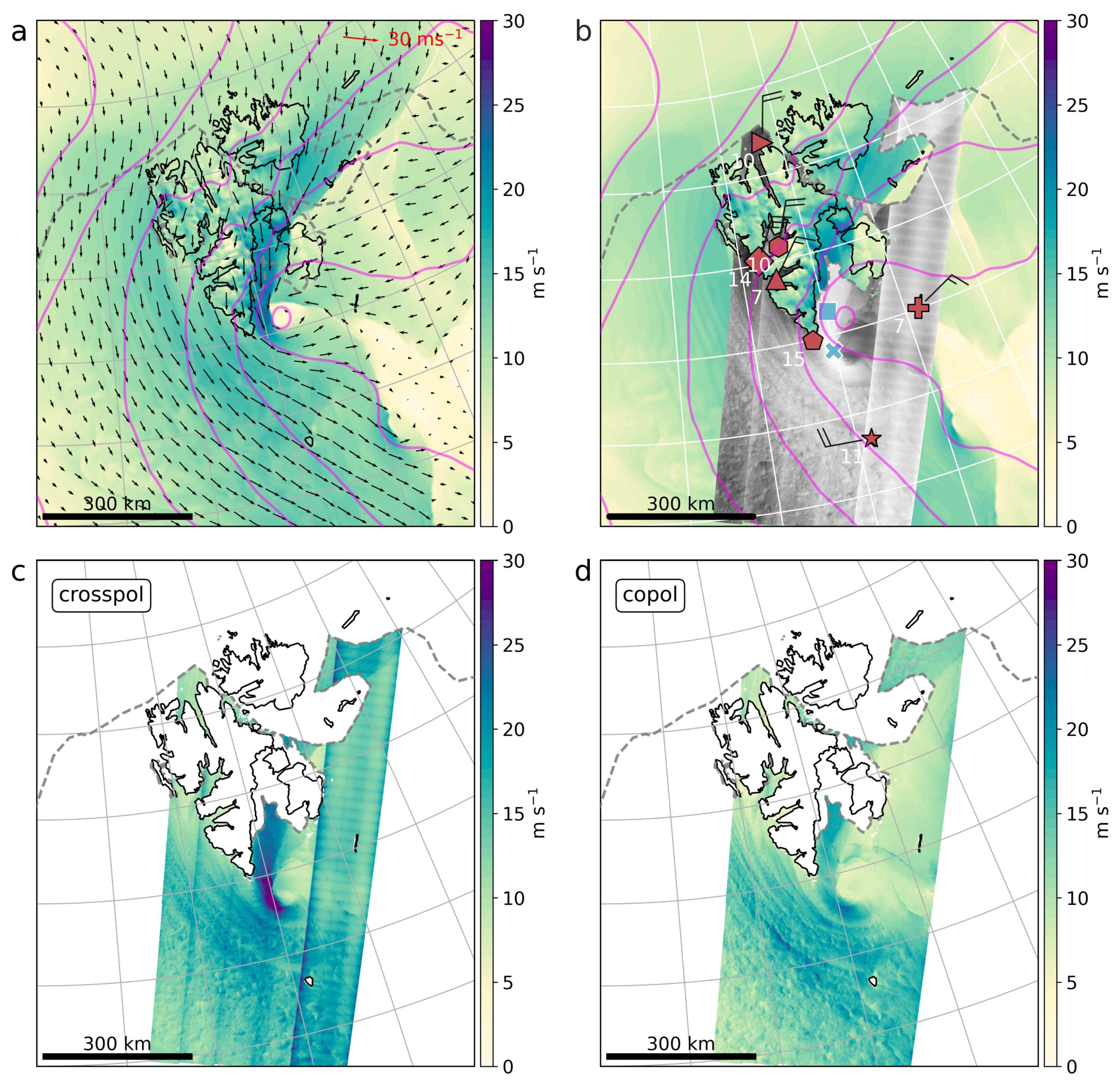
Here, a polar low case is presented that was observed by the SAR aboard the Sentinel-1 B satellite at 06 utc 26 December 2018. This case was chosen because of the distinct mismatch of about 80 km between the SAR observation of the polar low and the corresponding AROME-Arctic representation, and because it formed close to the archipelago of Svalbard, where a reasonably dense observational network of coastal, ground weather stations is present. These weather stations provide independent observations in close spatial vicinity to SAR ocean backscatter measurements (stations are shown in Figure 2b). The polar low formed inside a large fjord in the south of Svalbard close to sea ice and land. The presence of sea ice and land pose a major challenge to wind retrieval from remote sensing observations, especially so for those with lower spatial resolution than SAR, such as scatterometers. Land, and areas covered by sea ice, have to be excluded from wind retrieval since their associated high reflectivity values are not related to the surface wind. Here a manually produced sea ice chart from MET Norway is used to exclude areas that are contaminated by sea ice before the wind retrieval is applied. The dashed, grey line in Figure 2a,b indicates the sea ice border. The position of the polar low, as represented in the AROME-Arctic model, is indicated by the 10-m wind field and the sea surface pressure field shown in Figure 2a (10-m wind field is shown by colour shading and vectors, and sea surface pressure by magenta isobars with 4-hPa increments). The polar low centre, reaching a pressure of 987 hPa, is located at the entrance of the fjord, and the most intense wind speed of 24 m s lies along the coast to the west of the centre. The model wind is overlaid by a masked, greyscale image of crosspol backscatter in Figure 2b. Bright areas generally indicate high reflectivity and therefore high wind speed, except for signal noise that causes e.g., the straight bright lines that are visible in Figure 2b. Weather stations are shown by red station symbols with black wind barbs and white numbers indicating the measured wind. Even though model and radar observations are valid for the same time, the polar low centre in the radar image is located about 80 km further to the south than represented by the model (see Figure 2b and Figure 3f). In the radar image the brightest area, hence the strongest wind, wraps around the southwestern side of the centre. Figure 2c,d show results from the copol- and crosspol wind speed retrievals, respectively. The crosspol retrieval in Figure 2c closely resembles the reflectivity image, regrettably also with respect to the lines representing an artefact of strong instrument noise. While the wind field of the copol retrieval shown in Figure 2d shows hardly any visible traces of instrument noise, it contains some artefacts close to the polar low centre that originate from the misplaced model wind direction that is used in the classical copol retrieval (this is discussed in more detail in Section 3.2). In addition to these artefacts, the copol retrieval produces a less pronounced area of high wind speed on the south-west side of the polar low centre compared to the crosspol retrieval.
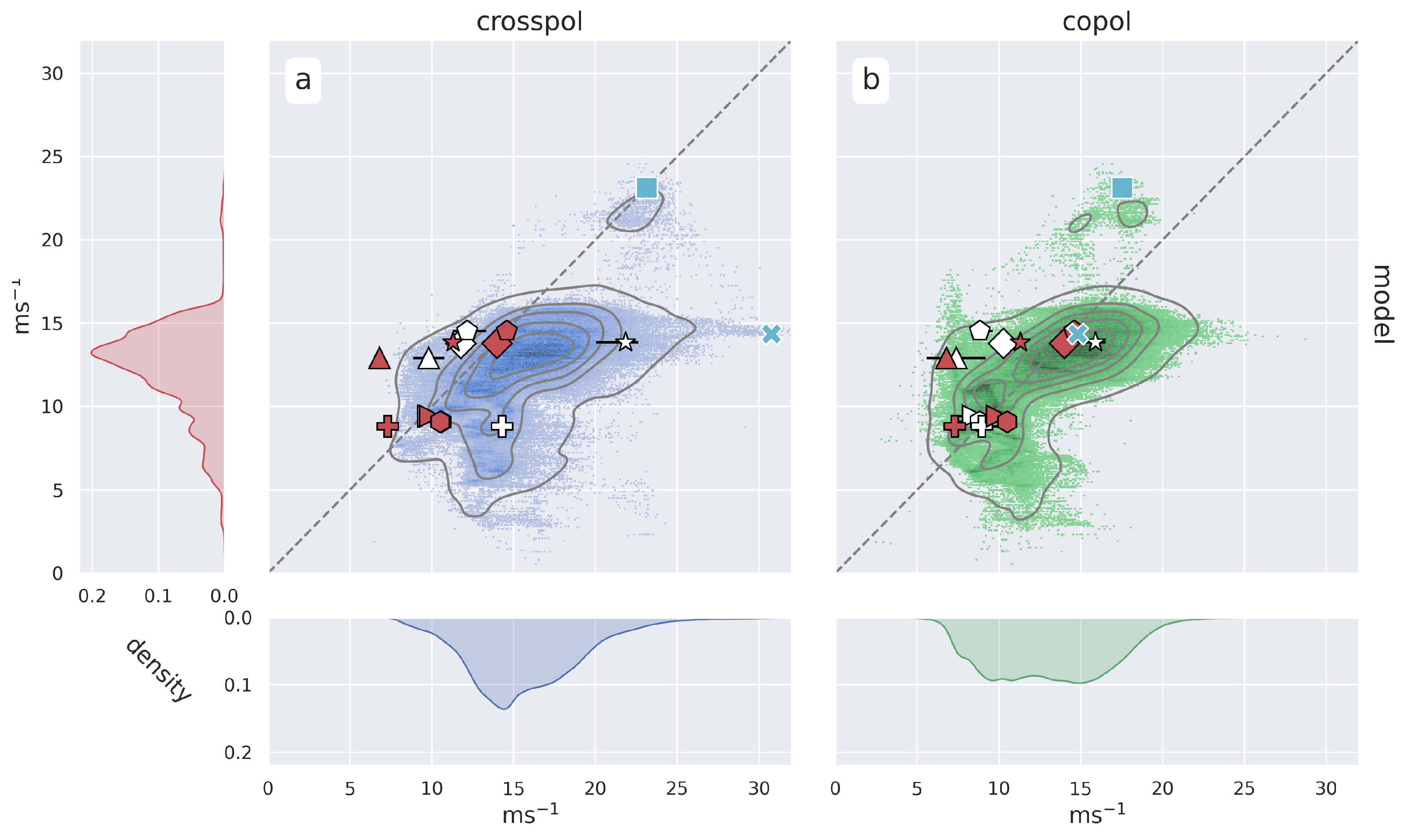
A quantitative comparison of the two wind speed retrievals with the corresponding AROME-Arctic model simulation that was resampled to the SAR grid, is shown in Figure 4. The plain wind speed distributions (rectangular panels in Figure 4) show a pronounced peak for the model (red) around 13 m s while both SAR retrievals (crosspol, MS1A in blue and copol, CMODH in green) have broader wind speed distributions. The highest modelled wind speeds, above 20 m s, are found west of the polar low centre and match with corresponding wind speeds from the collocated crosspol retrieval (square markers in Figure 2b and Figure 4a). Collocated wind speeds of the copol retrieval are about 5 m s lower than the maximum winds from the model simulation (Figure 4b).
The distinct peak around 13 m s in the model wind speed distribution originates from the uniform part of the modelled wind field south of Svalbard (cf. Figure 2a). The interpretation of the SAR-retrieved wind speeds that correspond with this uniform part of the model wind field can be separated into a physically meaningful part and errors in the wind retrieval. The physical interpretation of higher retrieved wind speeds compared to the model is the following: As a result of the northward misplacement of the polar low in the model, the highest SAR-retrieved wind speeds are extending into an area of moderate model wind speeds. In addition to that, the crosspol retrieval reaches wind speeds above 30 m s, much higher than the model simulation (x markers in Figure 2b and Figure 4a). Apart from the spatial mismatch, the larger wind speed variation of the SAR retrievals compared to the model can partly be attributed to small-scale variability, such as downdrafts from the widespread convection that is not resolved by the model physics (seen in the southern half of the wind retrievals in Figure 2c,d).
The other reason for a broader wind speed distribution of the SAR retrievals are errors in the retrieval process as well as instrument noise. For the crosspol wind speed retrieval, clearly the biggest issue is the low signal-to-noise ratio, meaning that for areas of low wind speed or strong instrument noise, the backscatter signal is indistinguishable from the instrument noise. This is especially true at sub-swath boundaries and for the lowest incidence sub-swath where the noise is strongest (see Figure 2b). Areas of strong noise lead to retrieved wind speeds that are too high. This is seen as straight lines in Figure 2c. In the case of the copol retrieval, signal saturation occurs at high wind speeds. That is, approaching saturation, the rate at which copol radar backscatter increases becomes small with increasing wind speeds. Another source of error of the copol wind retrieval results from the use of auxiliary wind direction information from the model. Any deviation of the modelled wind direction from the true wind direction results in an error of the retrieved wind speed. This is especially true for high wind speeds when the copol signal is approaching saturation as demonstrated in the following Section 3.2.
Wind speed observations from the seven weather stations that are shown as red symbols in Figure 2b are plotted against their corresponding model wind speed in Figure 4a,b. White markers of the same shape show the mean SAR retrieved wind speed of a 3 km radius around the station versus modelled wind speed at the station. Error bars indicate the variability of the retrieved wind within the 3 km radius of the station. The weather stations that lie inside the first sub-swath, the area most affected by instrument noise (star and cross markers in Figure 4a), are the ones where the values from the crosspol retrieval deviate most from the in situ observations. The measurement site closest to the polar low centre, pentagon marker, is the one for which the copol retrieval deviates most from the observation. The observed wind speed at the station marked with the triangle is closer to both SAR-retrievals than to the model. The latter simulated 7 m s higher wind speed than the observation. This could be due to a shallow stable boundary layer not captured by the model. The triangle station is located in a narrow fjord with complex topography (see Figure 2b) and is known to be misrepresented by AROME-Arctic under stable conditions. The observations presented here are too scarce and too uncertain to draw firm conclusions. However, they represent independent samples of the wind field that confirm the noise-problem of the crosspol wind retrievals and hint towards the potential strength of SAR to reveal stable shallow boundary layers that NWP models struggle to predict.
3.2. Information Content of SAR
The combination of copol backscatter and a priori wind from NWP, as introduced in Section 2.4, is the most established method to retrieve wind from SAR images. The European Space Agency applies this method to produce their widely used Sentinel-1 Ocean Wind Fields. As long as the surface wind field is moderately strong, uniform, and far away from steep coastal topography it is likely that the real wind direction is simulated well by the model and therefore the classical wind retrieval yields good results. However, this method uses only the information contained in the copol backscatter signal and relies heavily on a correct a priori wind direction.
For the retrieval of complex, mesoscale wind fields of polar lows with the classical copol retrieval, correct a priori wind direction can only be provided by a numerical model with high enough resolution to correctly simulate polar lows. Unfortunately, even a small spatial mismatch between the sharp wind gradients of a polar low captured by SAR observations and the corresponding model simulation can potentially lead to double penalty errors: imagine using a priori wind direction from a course-resolution model that does not at all simulate a polar low, but represents only the large-scale background flow. This situation would result in one-time errors from incorrect wind direction. Using the a priori wind direction of a high-resolution model that predicts sharp gradients of a polar low in an incorrect location is potentially penalised twice, once for failing to simulate a polar low that is indicated by the SAR observation, and once more for simulating a polar low where it should not be present according to the SAR-observation. To avoid such double penalty errors, we suggest exploiting all wind information contained in the SAR image without using any a priori wind direction. Only if necessary, should auxiliary wind information be used in a separate processing step to, e.g., remove ambiguities.
We propose to supplement the wind information contained in copol backscatter with wind speed information from the crosspol backscatter at high wind speeds and the Doppler shift. This can partly replace external wind direction information. These three sources of information can be combined as cost function terms in the same type of probabilistic retrieval that was presented in Section 2.4 omitting the a priori term. Such a cost function could read:
Note that the GMFs for copol backscatter and Doppler centroid anomaly, respectively and , are functions of the full wind vector , hence wind speed and direction. Contrarily, the crosspol GMF, , is a function of wind speed only. , and are the measured copol backscatter in horizontal polarisation, the crosspol backscatter, and the measured Doppler centroid anomaly, respectively. The corresponding Gaussian error standard deviations in the denominators are , , and . Previously the following constant values have been suggested for those errors 0.1 dB [7] and 5 Hz [30]. To rely on crosspol backscatter only in areas of strong signal and low noise a variable that depends on the local signal-to-noise ratio is applied here following the approach in [7].
For SAR-observed , and values at a given location, the minima of the three cost function terms in Equation (2) can be represented by contour lines of the respective GMFs at the measured values (Figure 1a–c). Figure 3a–e show those lines at the five locations indicated in Figure 3f for the example polar low that was presented in the previous section. For each location that is marked in Figure 3f, the corresponding copol (green), crosspol (blue), and DCA contours (orange) are shown together with the AROME-Arctic wind vector for the same location (empty grey symbol). For every location the ambiguous wind vectors from a probabilistic retrieval that minimises Equation (2) are indicated by the filled red symbols in Figure 3a–e and red wind arrows in Figure 3f. The orientation of the red reference arrow in the upper right corner of Figure 3f shows the 0 direction towards the radar. Isobars of sea level pressure (magenta contours) and the wind vectors from AROME-Arctic in Figure 3f demonstrate the spatial mismatch of about 80 km between the polar low observed by SAR and its representation by the AROME-Arctic model. Note that the blue line in Figure 3a–e corresponds to the wind speed of the crosspol retrieval at the extracted location. The wind vector of the classical copol wind retrieval using a priori wind direction from AROME-Arctic corresponds to the intersection of the grey, dashed line through the AROME-Arctic marker and the green copol line in Figure 3a–e.
The location marked with the triangle symbol in Figure 3f lies close to the centre of the model polar low where AROME-Arctic predicted a wind speed of 5 m s blowing almost directly in the opposite direction to the radar as can be seen by the empty grey triangle in Figure 3a. From the brightness of the underlying greyscale SAR image, it is quite obvious that the location marked with the triangle in reality experienced a strong northeasterly wind, which corresponds better with the retrieved ambiguity at 17 m s and 130° in Figure 3a. Note that in the classical copol retrieval shown in Figure 2d, the AROME-Arctic a priori wind vector is used as auxiliary information during wind retrieval. The retrieved wind vector of the classical copol retrieval is therefore close to the intersection of the green line with the vertical, grey, dashed line through the grey marker in Figure 3a–e. Using the wrong wind direction from the model at this location leads to a dampened wind speed.
At the location marked with the square symbol in Figure 3f, the model and the crosspol retrieval show the same wind speed, while the copol wind retrieval with the model wind direction leads to a 5 m s lower wind speed (Figure 3b, also seen in Figure 4a,b). For the ambiguous wind retrieval at this location, one of the ambiguities seems to match the real wind direction again and the wind speed lies between the copol and crosspol retrievals.
Increasing wind speed increases the potential error caused by a wrong a priori wind direction input to the classical copol wind retrieval. The cross symbol in Figure 3f marks the area of maximum crosspol backscatter intensity and largest local signal-to-noise ratio. As shown in Figure 3c and Figure 4, crosspol and copol retrieval differ at this location by 17 m s. In the SAR-only retrieval, the high signal-to-noise ratio results in relatively high weight of the crosspol term of Equation (2) relative to the copol term that has constant weight. Therefore, the wind speed of the SAR-only retrieval is close to the crosspol retrieval at this location.
Since the wind directions of AROME-Arctic, and one of the ambiguous wind vectors almost match at the location marked with the circle symbol in Figure 3f, the retrieved wind speed of the classical copol retrieval is close to the ambiguous SAR-only retrieval (Figure 3d). However, note that, at this location, a slightly different a priori wind direction would result in dramatically different wind speed for the copol retrieval.
Last, the diamond symbol in Figure 3f marks a location with very low signal-to-noise ratio of the crosspol backscatter. Here, the crosspol term in Equation (2) weights accordingly low, and the SAR-only wind speed is close to the green copol contour in Figure 3e.
A mismatch between the SAR image and numerical model of the order that is presented here (Figure 3f) is enough to achieve wind direction errors between 0 and 180°, covering the full range of possible errors for the wind speed component of the classical copol retrieval. Therefore any wind retrieval that indiscriminately relies on such auxiliary wind direction input is corrupted. Figure 3g shows the full wind field of the SAR-only retrieval with the black and white arrows indicating the ambiguous wind directions. The combination of the three sources of information, copol, crosspol, and DCA seems to yield realistic wind speeds, and one of the wind direction ambiguities is qualitatively always aligned with the real wind direction.
4. Discussion
The classical wind retrieval that combines copol radar backscatter with a priori wind information from a numerical model is a good method for many applications. However, our analysis of a polar low event that was misrepresented by the AROME-Arctic model shows that the potential benefits of high-resolution SAR observations cannot be reached with current wind retrieval methods that heavily rely on a correct representation of the wind direction by a numerical model. Currently the Gaussian error standard deviation of the a priori term in Equation (1), , in the classical copol wind retrieval is assumed to be constant. Thereby, it is assumed that the model wind is equally correct everywhere which appears to be a poor assumption for complex mesoscale wind fields. The assumption of constant model error can only be relaxed if the DCA or alternative wind direction information is available as a substitute for the model wind direction.
The SAR-only retrieval presented here still follows the convention of constant error terms and [7,30] in Equation (2). Future work is dedicated to a thorough investigation of meaningful variable error terms which will presumably improve the quality of the SAR-only retrieval due to optimised weights of the cost function terms. In addition, a meaningful treatment of variable errors will provide a total error of the SAR-only wind retrieval, which is required for assimilation into numerical weather prediction models.
In a broader context, it appears reasonable to keep separate the extraction of wind information from the SAR image in an ambiguous SAR-only wind retrieval, such as the one suggested here, and then optionally use numerical model data for ambiguity removal. By doing so, the ambiguous wind field remains independent of numerical models and can be used as observations in assimilation or model validation. Here, it is worth noting that assimilation systems can handle ambiguous wind fields, and that, e.g., ambiguous winds retrieved from scatterometer observations are routinely assimilated at ECMWF. A study on the impact of assimilating ambiguous SAR winds into a high-resolution NWP is in preparation.
Most applications for SAR-derived wind fields likely still prefer unambiguous wind directions which calls for future investigations in ambiguity removal. Such attempts might revisit the extraction of linear features or a more nuanced consideration of model wind directions.
Furthermore, the SAR-only method presented here has to be refined, validated, and adapted for the use on IW backscatter images including the new crosspol GMF for the Sentinel-1 IW mode [31]. If assimilation experiments with ambiguous SAR winds show a positive effect on weather predictions, a fast algorithm for operational use needs to be developed.
5. Conclusions
Two common wind retrieval techniques are applied to SAR dual polarisation observations of the sea surface backscatter during a polar low event with complex wind structure. The goal is to evaluate the performance of these techniques for such rapidly evolving, intense mesoscale cyclones. Furthermore, we advocate a new wind retrieval technique that exploits the information content of SAR observations to a larger extend than existing methods do. These are the main findings:
- Current wind retrieval methods that retrieve wind from a single product, copol or crosspol, or rely on auxiliary wind information form numerical models are not suitable to derive a surface wind field from SAR observations of highly variable wind environments, such as polar lows, due to potentially large errors caused by the use of incorrect auxiliary wind direction information or high instrument noise.
- Comprehensive utilisation of, thus far, neglected wind direction information gathered from a combination of copol and crosspol backscatter, and the Doppler centroid anomaly can replace the need for auxiliary wind direction information during wind vector retrieval and minimise the effect of instrument noise. The resulting new SAR-only wind retrieval yields a wind field with a directional ambiguity that is independent of a priori information from NWP models. Thereby, the SAR-only wind retrieval is free from errors caused by incorrect auxiliary wind direction provided by models that are likely to misrepresent the details of complex wind structures.
- High-resolution surface wind fields of dynamically changing weather events, such as polar lows obtained from this unsupervised wind retrieval can potentially improve weather predictions of these events by providing small-scale observations for the data assimilation process of mesoscale NWP models.
Author Contributions
Conceptualisation, all authors contributed; methodology, M.T.; software, M.T. and H.J.; writing—original draft preparation, M.T.; writing—review and editing, all authors contributed; visualisation, M.T. All authors have read and agreed to the published version of the manuscript.
Funding
This research was funded by the Centre of Integrated Remote Sensing and Forecasting for Arctic Operations (CIRFA) under the Research Council of Norway (RCN), grant number 237906.
Data Availability Statement
The Norwegian meteorological institute provides free access to meteorological data from the AROME-Arctic model, as well as in situ observations at https://thredds.met.no/thredds/catalog/aromearcticarchive/2018/12/26/catalog.html (accessed November 2021) and at https://frost.met.no/index.html (accessed November 2021). SAR data can be searched and downloaded freely at https://search.asf.alaska.edu (accessed November 2021).
Acknowledgments
Thanks to the meteorological institute of Norway and to the Norwegian Research Centre AS (NORCE) for providing support and access to their systems, which was a integral contribution to making this work possible. We thank the two anonymous reviewers for their comments and Sam Black for proofreading the manuscript.
Conflicts of Interest
The authors declare no conflict of interest.
Abbreviations
The following abbreviations are used in this manuscript:
| SAR | synthetic aperture radar |
| GMF | geophysical model function |
| copol | co-polarised; same polarisation plane for transmitted and received signal |
| HH (VV) | horizontally (vertically) polarised transmitted and received radiation |
| crosspol | cross-polarised; 90° different polarisation planes for transmission and reception |
| HV (VH) | horizontal and vertical polarisation for transmission and reception (or opposite) |
| NWP | numerical weather prediction |
| ECMWF | European Centre for Medium-Range Weather Forecasts |
References
- Donnelly, W.J.; Carswell, J.R.; McIntosh, R.E.; Chang, P.S.; Wilkerson, J.; Marks, F.; Black, P.G. Revised ocean backscatter models at C and Ku band under high-wind conditions. J. Geophys. Res. Ocean. 1999, 104, 11485–11497. [Google Scholar] [CrossRef]
- Wackerman, C.C.; Rufenach, C.L.; Shuchman, R.A.; Johannessen, J.A.; Davidson, K.L. Wind vector retrieval using ERS-1 synthetic aperture radar imagery. IEEE Trans. Geosci. Remote Sens. 1996, 34, 1343–1352. [Google Scholar] [CrossRef]
- Lehner, S.; Horstmann, J.; Koch, W.; Rosenthal, W. Mesoscale wind measurements using recalibrated ERS SAR images. J. Geophys. Res. Ocean. 1998, 103, 7847–7856. [Google Scholar] [CrossRef]
- Horstmann, J.; Schiller, H.; Schulz-Stellenfleth, J.; Lehner, S. Global wind speed retrieval from SAR. IEEE Trans. Geosci. Remote. Sens. 2003, 41, 2277–2286. [Google Scholar] [CrossRef] [Green Version]
- Vachon, P.W.; Wolfe, J. C-band cross-polarization wind speed retrieval. IEEE Geosci. Remote. Sens. Lett. 2010, 8, 456–459. [Google Scholar] [CrossRef]
- Zhang, B.; Perrie, W. Cross-polarized synthetic aperture radar: A new potential measurement technique for hurricanes. Bull. Am. Meteorol. Soc. 2012, 93, 531–541. [Google Scholar] [CrossRef] [Green Version]
- Mouche, A.A.; Chapron, B.; Zhang, B.; Husson, R. Combined co-and cross-polarized SAR measurements under extreme wind conditions. IEEE Trans. Geosci. Remote Sens. 2017, 55, 6746–6755. [Google Scholar] [CrossRef]
- Zhang, B.; Fan, S.; Mouche, A.; Zhang, G.; Perrie, W. Synergistic Measurements of Hurricane Wind Speeds and Directions from C-band Dual-Polarization Synthetic Aperture Radar. In Proceedings of the IGARSS 2019-2019 IEEE International Geoscience and Remote Sensing Symposium, Yokohama, Japan, 28 July–2 August 2019; pp. 4618–4621. [Google Scholar]
- Koch, W. Directional analysis of SAR images aiming at wind direction. IEEE Trans. Geosci. Remote Sens. 2004, 42, 702–710. [Google Scholar] [CrossRef]
- Lin, H.; Xu, Q.; Zheng, Q. An overview on SAR measurements of sea surface wind. Prog. Nat. Sci. 2008, 18, 913–919. [Google Scholar] [CrossRef]
- Mouche, A.A.; Collard, F.; Chapron, B.; Dagestad, K.F.; Guitton, G.; Johannessen, J.A.; Kerbaol, V.; Hansen, M.W. On the use of Doppler shift for sea surface wind retrieval from SAR. IEEE Trans. Geosci. Remote Sens. 2012, 50, 2901–2909. [Google Scholar] [CrossRef]
- Rasmussen, E.A. Polar lows. In A Half Century of Progress in Meteorology: A Tribute to Richard Reed; Springer: Berlin/Heidelberg, Germany, 2003; pp. 61–78. [Google Scholar]
- Mile, M.; Randriamampianina, R.; Marseille, G.J.; Stoffelen, A. Supermodding—A special footprint operator for mesoscale data assimilation using scatterometer winds. Q. J. R. Meteorol. Soc. 2021, 147, 1382–1402. [Google Scholar] [CrossRef]
- Lu, Y.; Zhang, B.; Perrie, W.; Mouche, A.; Zhang, G. CMODH Validation for C-Band Synthetic Aperture Radar HH Polarization Wind Retrieval Over the Ocean. IEEE Geosci. Remote Sens. Lett. 2020, 18, 102–106. [Google Scholar] [CrossRef]
- Said, F.; Johnsen, H.; Chapron, B.; Engen, G. An ocean wind Doppler model based on the generalized curvature ocean surface scattering model. IEEE Trans. Geosci. Remote. Sens. 2015, 53, 6632–6638. [Google Scholar] [CrossRef] [Green Version]
- ESA. Sentiel-1 Technical Guide. 2021. Available online: https://sentinel.esa.int/web/sentinel/missions/sentinel-1 (accessed on 18 May 2021).
- Müller, M.; Batrak, Y.; Kristiansen, J.; Køltzow, M.A.; Noer, G.; Korosov, A. Characteristics of a convective-scale weather forecasting system for the European Arctic. Mon. Weather. Rev. 2017, 145, 4771–4787. [Google Scholar] [CrossRef]
- Seity, Y.; Brousseau, P.; Malardel, S.; Hello, G.; Bénard, P.; Bouttier, F.; Lac, C.; Masson, V. The AROME-France convective-scale operational model. Mon. Weather. Rev. 2011, 139, 976–991. [Google Scholar] [CrossRef] [Green Version]
- Stoll, P.J.; Valkonen, T.M.; Graversen, R.G.; Noer, G. A well-observed polar low analysed with a regional and a global weather-prediction model. Q. J. R. Meteorol. Soc. 2020, 146, 1740–1767. [Google Scholar] [CrossRef]
- Müller, M.; Homleid, M.; Ivarsson, K.I.; Køltzow, M.A.; Lindskog, M.; Midtbø, K.H.; Andrae, U.; Aspelien, T.; Berggren, L.; Bjørge, D.; et al. AROME-MetCoOp: A Nordic convective-scale operational weather prediction model. Weather. Forecast. 2017, 32, 609–627. [Google Scholar] [CrossRef]
- Zhang, B.; Mouche, A.; Lu, Y.; Perrie, W.; Zhang, G.; Wang, H. A geophysical model function for wind speed retrieval from C-band HH-polarized synthetic aperture radar. IEEE Geosci. Remote. Sens. Lett. 2019, 16, 1521–1525. [Google Scholar] [CrossRef]
- Portabella, M.; Stoffelen, A.; Johannessen, J.A. Toward an optimal inversion method for synthetic aperture radar wind retrieval. J. Geophys. Res. Ocean. 2002, 107, 1. [Google Scholar] [CrossRef]
- Adamo, M.; Rana, F.M.; De Carolis, G.; Pasquariello, G. Assessing the Bayesian inversion technique of C-band synthetic aperture radar data for the retrieval of wind fields in marine coastal areas. J. Appl. Remote Sens. 2014, 8, 083531. [Google Scholar] [CrossRef]
- Wang, H.; Yang, J.; Mouche, A.; Shao, W.; Zhu, J.; Ren, L.; Xie, C. GF-3 SAR ocean wind retrieval: The first view and preliminary assessment. Remote Sens. 2017, 9, 694. [Google Scholar] [CrossRef] [Green Version]
- Moiseev, A.; Johnsen, H.; Johannessen, J.; Collard, F.; Guitton, G. On Removal of Sea State Contribution to Sentinel-1 Doppler Shift for Retrieving Reliable Ocean Surface Current. J. Geophys. Res. Ocean. 2020, 125, e2020JC016288. [Google Scholar] [CrossRef]
- Engen, G.; Johnsen, H.; Larsen, Y. Sentinel-1 geophysical doppler product-performance and application. In Proceedings of the EUSAR 2014, 10th European Conference on Synthetic Aperture Radar, Berlin, Germany, 3–5 June 2014; pp. 1–4. [Google Scholar]
- Engen, G.; Johnsen, H. Sentinel-1 Doppler and Ocean Radial Velocity Algorithm Definition. Image 2015, 19, 62. [Google Scholar]
- Chapron, B.; Collard, F.; Ardhuin, F. Direct measurements of ocean surface velocity from space: Interpretation and validation. J. Geophys. Res. Ocean. 2005, 110. [Google Scholar] [CrossRef]
- Saïd, F.; Johnsen, H. Ocean surface wind retrieval from dual-polarized SAR data using the polarization residual Doppler frequency. IEEE Trans. Geosci. Remote. Sens. 2013, 52, 3980–3990. [Google Scholar] [CrossRef] [Green Version]
- Hansen, M.W.; Collard, F.; Dagestad, K.F.; Johannessen, J.A.; Fabry, P.; Chapron, B. Retrieval of sea surface range velocities from Envisat ASAR Doppler centroid measurements. IEEE Trans. Geosci. Remote Sens. 2011, 49, 3582–3592. [Google Scholar] [CrossRef]
- Gao, Y.; Sun, J.; Zhang, J.; Guan, C. Extreme Wind Speeds Retrieval Using Sentinel-1 IW Mode SAR Data. Remote Sens. 2021, 13, 1867. [Google Scholar] [CrossRef]
Figure 2.
AROME-Arctic model simulation as well as weather station observations and Sentinel-1 crosspol SAR backscatter of an example polar low at 06 utc 26 December, 2018, close to the archipelago of Svalbard. (a) AROME-Arctic wind field at 10 m AGL (arrows and colour shading in m s) and isobars of sea level pressure (magenta contour lines with 4-hPa increments). The dashed, grey line shows the sea ice edge (sea ice concentration = 0) and indicates the boundary of the area within which ice-contaminated SAR observations were removed. (b) as in (a), but overlaid with ground weather stations (red station symbols with black wind barbs and white wind speed in m s) and SAR crosspol backscatter intensities (grey shading in dB, bright indicates high values). The blue square and x symbols indicate the areas of maximum wind speed simulated by the AROME-Arctic model and the crosspol retrieval. (c,d) show retrieved wind speed (colour shading in m s) from two established wind retrievals that use the crosspol backscatter, and a combination of copol backscatter and the a priori wind direction of the AROME-Arctic model, respectively.

Figure 3.
(a–e) illustration of the three cost function terms in Equation (2) for five selected locations that are marked in (f). The blue, green and orange lines in (a–e) represent the crosspol-, copol-, and Doppler terms of Equation (2), respectively. The corresponding AROME-Arctic wind vector for each location is marked with an empty grey symbol and ambiguous wind vectors from the SAR-only retrieval that minimises Equation (2) are marked by red symbols in (a–e). The direction of 0°, wind blowing towards the radar, is marked by the red reference arrow in (f,g). Angles increase in clockwise direction. (f) SAR crosspol backscatter image (grey shading in dB, bright indicates high values) overlaid with sea level pressure (magenta contours) and wind arrows from AROME-Arctic. Blue symbols mark the locations of (a–e) and the pairs of red arrows show the ambiguous wind vectors of the SAR-only retrieval. The complete wind field of the SAR-only retrieval is shown in (g) with white and black arrows indicating the two wind direction solutions.

Figure 4.
Comparison of retrieved wind speed from the crosspol (a) and copol (b) wind retrievals shown in Figure 2c,d, and collocated wind speed from the AROME-Arctic model. The darker colour shows higher point density, as do the contour lines of the kernel density estimation. The narrow panels on the left and bottom show the associated wind speed distributions. Filled red symbols show weather station observations with the observed wind speed on the horizontal axis and the corresponding model wind speed on the vertical axis. Filled blue symbols with error bars show the mean and variance of the retrieved wind speed within a 3 km radius of the weather stations on the horizontal axis against the corresponding model wind speed at the station on the vertical axis. Filled green symbols show the same for the copol retrieval.

Publisher’s Note: MDPI stays neutral with regard to jurisdictional claims in published maps and institutional affiliations. |
© 2021 by the authors. Licensee MDPI, Basel, Switzerland. This article is an open access article distributed under the terms and conditions of the Creative Commons Attribution (CC BY) license (https://creativecommons.org/licenses/by/4.0/).
Share and Cite
MDPI and ACS Style
Tollinger, M.; Graversen, R.; Johnsen, H. High-Resolution Polar Low Winds Obtained from Unsupervised SAR Wind Retrieval. Remote Sens. 2021, 13, 4655. https://0-doi-org.brum.beds.ac.uk/10.3390/rs13224655
AMA Style
Tollinger M, Graversen R, Johnsen H. High-Resolution Polar Low Winds Obtained from Unsupervised SAR Wind Retrieval. Remote Sensing. 2021; 13(22):4655. https://0-doi-org.brum.beds.ac.uk/10.3390/rs13224655
Chicago/Turabian StyleTollinger, Mathias, Rune Graversen, and Harald Johnsen. 2021. "High-Resolution Polar Low Winds Obtained from Unsupervised SAR Wind Retrieval" Remote Sensing 13, no. 22: 4655. https://0-doi-org.brum.beds.ac.uk/10.3390/rs13224655
Note that from the first issue of 2016, this journal uses article numbers instead of page numbers. See further details here.