
Stitching and Geometric Modeling Approach Based on Multi-Slice Satellite Images
by
 , , ,
, , ,
Longhui Wang
1 ,
,
Yan Zhang
1,*,
Tao Wang
1,
Yongsheng Zhang
1,
Zhenchao Zhang
2,
Ying Yu
1 and
Lei Li
1 1
Geospatial Information Institute, Information Engineering University, Zhengzhou 450001, China
2
Department of Earth Observation Science, Faculty ITC, University of Twente, 7511 AE Enschede, The Netherlands
*
Author to whom correspondence should be addressed.
Remote Sens. 2021, 13(22), 4663; https://0-doi-org.brum.beds.ac.uk/10.3390/rs13224663
Submission received: 21 October 2021
/
Revised: 13 November 2021
/
Accepted: 15 November 2021
/
Published: 19 November 2021
(This article belongs to the Special Issue Remote Sensing and Digital Twins)
Abstract
:Time delay and integration (TDI) charge-coupled device (CCD) is an image sensor for capturing images of moving objects at low light levels. This study examines the model construction of stitched TDI CCD original multi-slice images. The traditional approaches, for example, include the image-space-oriented algorithm and the object-space-oriented algorithm. The former indicates concise principles and high efficiency, whereas the panoramic stitching images lack the clear geometric relationships generated from the image-space-oriented algorithm. Similarly, even though the object-space-oriented algorithm generates an image with a clear geometric relationship, it is time-consuming due to the complicated and intensive computational demands. In this study, we developed a multi-slice satellite images stitching and geometric model construction method. The method consists of three major steps. First, the high-precision reference data assist in block adjustment and obtain the original slice image bias-corrected RFM to perform multi-slice image block adjustment. The second process generates the panoramic stitching image by establishing the image coordinate conversion relationship from the panoramic stitching image to the original multi-slice images. The final step is dividing the panoramic stitching image uniformly into image grids and employing the established image coordinate conversion relationship and the original multi-slice image bias-corrected RFM to generate a virtual control grid to construct the panoramic stitching image RFM. To evaluate the performance, we conducted experiments using the Tianhui-1(TH-1) high-resolution image and the Ziyuan-3(ZY-3) triple liner-array image data. The experimental results show that, compared with the object-space-oriented algorithm, the stitching accuracy loss of the generated panoramic stitching image was only 0.2 pixels and that the mean value was 0.799798 pixels, achieving the sub-pixel stitching requirements. Compared with the object-space-oriented algorithm, the RFM positioning difference of the panoramic stitching image was within 0.3 m, which achieves equal positioning accuracy.
1. Introduction
The spaceborne linear-array sensor is an indispensable carrier for remote sensing earth observation. Given the growing applications and uses of remote sensing technology, sensor performance, index, and imaging quality should meet more stringent requirements. Most optical sensors employ the spliced time delay and integration charge-coupled device (TDI CCD) technology in acquiring ground images to achieve high imaging quality and wide terrain coverage. It has a wide range of applications due to its outstanding imaging performance. For example, satellites such as IKONOS, QuickBird, WorldView-2, SPOT6/7, LandSat-8, “Tianhui-1 (TH-1)”, “Ziyuan-3 (ZY-3)”, “Gaofen-2”, and “Gaofen-7” [1,2,3,4,5,6,7] are equipped with these sensors. As the technology progresses, the spatial resolution of images has reached the sub-meter level. Therefore, the stitching processing of original multi-slice images and the construction of geometric models of panoramic stitching images cannot ignore stitching errors.
Along the flight direction of the satellite platform, the stitched TDI CCD sensor obtains original multi-slice images for earth observation. Multiple factors change the geometric quality of the original multi-slice images and the overlapping relationship of the adjacent slice, such as internal aberrations of the sensor, deflection angle control, platform tremor, and attitude angle errors. Consequently, imaging parameters require the on-orbit geometric calibration and the correction of the ground processing model. Taking the external and internal errors into account, including the bias of camera installation angle, time measurement errors, attitude measurement errors, orbit measurement errors and optical distortion of the camera lens, Xu et al. [8] applied the geometric calibration model to enhance the direct positioning performance and internal accuracy of the ZY-3 02 satellite triple linear-array. Wang et al. [9,10,11,12] recommended a self-calibration model suitable for images to eliminate the system positioning error and improve image stereo positioning accuracy. After geometric calibration, the upgraded image quality facilitates the subsequent high-quality stitching and geometric model construction of the original multi-slice images.
Current stitching algorithms classify two types: image-space-oriented and object-space-oriented. The image-space-oriented algorithm relies on automatic image matching to generate tie points and adopt specific stitching models to complete the stitching, such as interslice translation [13], piecewise affine transformation [14], and line integration time normalization [15]. The image-space-oriented algorithm is efficient and straightforward, relying solely on the image’s information, whereas the resulting panoramic stitched image lacks a clear geometric object-image relationship. The object-space-oriented algorithm is generated from the continuity of the object-space and generates the panoramic stitched image based on the strict geometric model of the sensor. Hu [15] proposed an object-space stitching algorithm for constructing a virtual TDI CCD line array according to the interslice imaging geometric constraint relationship between three inconsistent TDI CCDs fragments, discussed the sources of stitching errors, and validated the method through simulated data. Numerous studies [16,17,18,19] have explored the influence of topographic relief on the splicing accuracy and generated the rational function model (RFM) based on constructing a strict geometric model of the virtual line array. Pan et al. [20,21] optimized the stitching process and verified the method’s feasibility using ZY-1 02C satellite high-resolution images. Jiang et al. [22] set up a virtual camera model through the relative geometric inspection of the dual cameras of the Remote Sensing 24, achieving seamless stitching of the dual cameras. The object stitching algorithm has a strict and clear geometric object relationship, but the precise sensor parameters and data, such as orbital ephemeris, are often challenging to obtain, and the processing is difficult and time-consuming.
This study presents a method for stitching and the geometric model construction of multi-slice satellite images. Using the multi-slice image block adjustment, the proposed modeling approach takes advantage of high-precision reference data for control points, enhancing the positioning accuracy of the original multi-slice image RFM. The image segmental affine transformation model is applied to set the coordinate transformation relationship of the image points from the panoramic stitch image to the original segmented image. Finally, the panoramic stitching image is divided evenly into image grids. The established image coordinate conversion relationship and the original segmented image RFM compensation model are used to establish a virtual control grid of objects to construct the panoramic stitching image RFM.
2. Materials and Methods
2.1. Study Area and Data Acquisition
The research site is located in the Dengfeng area (34°27′ N, 113°02′ E) of Henan Province, Central China. The study area includes mountainous, hilly, and flat terrain with undulating topography. The region’s mean elevation is 350 m, while the maximum elevation is 1450 m.
Two different satellite image data were collected, TH-1 02 high-resolution (HR) image and ZY-3 01 triple linear-array image. Table 1 presents the detailed information of the experimental data, while Figure 1 shows the overview of the original multi-slice images. Data A use mechanical stitching, and there is a misalignment relationship of about 2114 pixels in the along-track direction in the adjacent slice. Data B are imaged by optical stitching, and the misalignment in the along-track direction in the adjacent slice is smaller. High-precision reference data, including digital orthophoto mapper (DOM) (resolution: 0.5 m) and digital elevation model(DEM) (resolution: 1 m), were also employed to match the reference points automatically.
2.2. Processing and Analysis
For multi-linear array images, the original multi-slice images were matched to obtain the tie points. Some filtered tie points were matched with the DOM, and the ground control points (GCPs) were acquired after interpolating the elevation values in the DEM. As for single-line array images, the original multi-slice images were directly matched with the DOM to obtain the GCPs. Adjacent slice images were automatically matched to obtain interslice tie points (ITPs) in the overlapping area. The SUFT algorithm applies automatic matching with a matching accuracy greater than 0.5 pixels.
For multi-linear array images as the ZY-3 satellite triple linear-array, its nadir view image comprises 3 CCDs, and the forward and backward view images are composed of 4 CCDs, respectively. The multi-slice images were matched by multi-view to obtain the tie points, and some of the tie points were screened and matched with the DOM with geographic information to obtain the corresponding ground point plane coordinates. The elevation values are interpolated in the DEM, which were used as control points after the elevation datum conversion.
With regard to single-linear array image, such as the TH-1 satellite HR image, is composed of 8 CCDs. The original slice image was directly matched with the DOM to obtain the control point plane coordinates, and the elevation value was interpolated and updated in the DEM.
The processing consists of three steps: (1) multi-slice images RFM block adjustment, (2) panoramic image stitching based on piecewise affine transformation model, (3) and panoramic stitching image RFM construction. Figure 2 shows the methodology flow chart and depicts the details of each step.
2.3. Multi-Slice Images RFM Block Adjustment
The satellite is calibrated on-orbit and eliminates the systematic errors of the inner and outer azimuth elements. However, after the satellite is in operation for a period of time, due to outer orientation data, observations have a specific systematic error, making geometric image positioning biased. Moreover, the RFM generated by the strict geographical model fitting also has a corresponding systematic error. The assistance of high- precision reference data can compensate for the systematic errors of each original slice image, thus improving the RFM positioning accuracy.
2.3.1. Bias-Corrected RFM
RFM connects the image coordinate with the corresponding object coordinate in the form of a polynomial ratio [23]. The definition is shown in Equation (1).
where, , , and are RFM parameters; and are usually 1; are normalized image coordinates; and are normalized object coordinates.
where, , , , and are the unnormalized coordinate; , , and are the image coordinate normalization parameters; , , , , and are the object coordinate normalization parameters.
Image compensation (IC) eliminates the systematic error of the image and is more theoretically rigorous than object compensation [24,25]. The affine transformation model is usually chosen as the image compensation model and is given by the expression:
where, are the systematic error compensation parameters for each slice image.
Therefore, the correction relationship between image and object coordinates is as follows:
where, , and .
2.3.2. RFM Block Adjustment
When the object of study is a multi-linear array image, the observations include two types of GCPs and tie points. Since the coordinates of the GCPs are precisely known, the unknown parameters of the error equation constructed only include the RFM image compensation parameters. In this case, Equation (4) is considered a linear equation, and the error equation is established as Equation (5). Image compensation eliminates the systematic error of the image and is more theoretically rigorous than object compensation [22,23]. Therefore, the affine transformation model is usually chosen as the image compensation model, given by the expression:
In addition to the RFM image compensation parameters, the tie point unknown parameters also contain its object coordinates. Equation (4) needs to be linearized, and the initial value of the tie point object coordinates can be obtained from the RFM space intersection. The tie point error equation is:
Combining Equations (5) and (6), the image compensation parameters and the object coordinates of the tie point are solved together and written in matrix form as follows:
where, is the residual vector of the error equation; is the vector of coefficient corrections of the image affine transformation; is the vector of corrections of the object coordinates of the tie point; and are the matrix of coefficients of the unknowns; is the constant term obtained from the calculation; and is the power matrix.
When the object of study is a single-linear array image, the observations consist of only GCPs, and the error equation can be established from Equation (5) in the form of a matrix, where the vector expressions are all consistent with Equation (7).
The control points and tie points establish the error equation using Equations (5) and (6), and the weight is fixed given the observation accuracy. The leveling operation yields the RFM image compensation model.
2.4. Panoramic Image Stitching Based on Piecewise Affine Transformation Model
The mounting relationship is introduced with three TDI CCDs as an example, as shown in Figure 3. The TDI CCDs are staggered in the focal plane with each slice length w pixels, spaced by dy pixels along the track direction, and overlapping dx pixels in the vertical track direction. The original multi-slice images are obtained by pushing and scanning along the flight direction.
2.4.1. Piecewise Affine Transformation Model
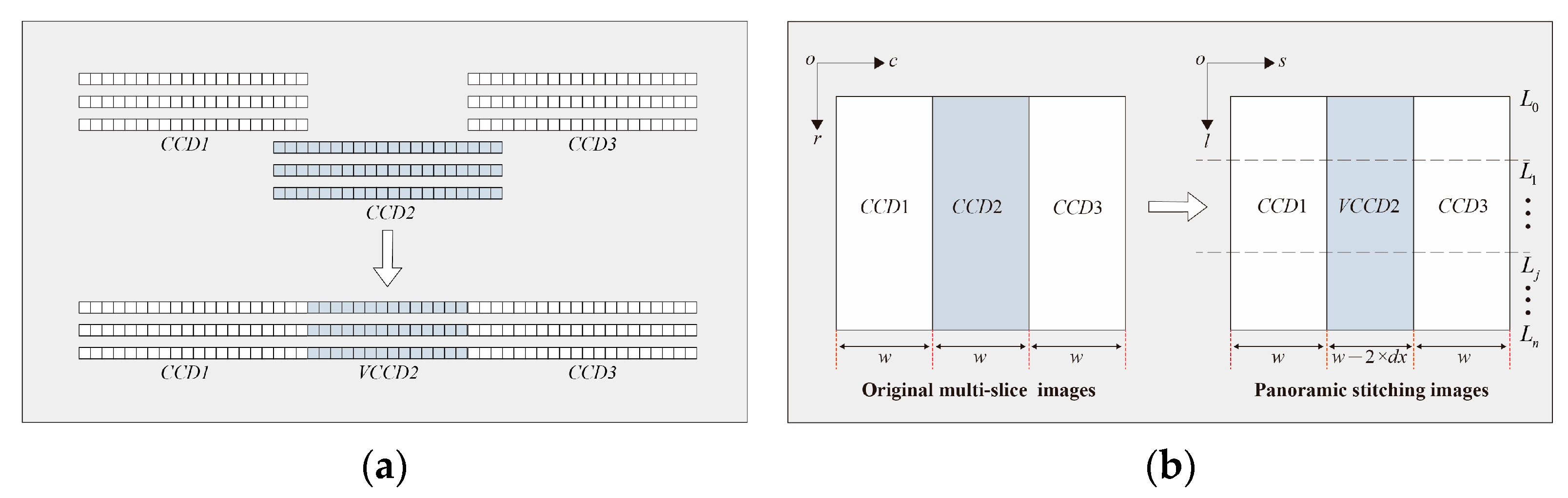
Acquired directly from three TDI CCDs that are strictly co-linear in the focal plane, the panoramic stitching image keeps the position of the odd slice image unchanged and embeds the even slice image between the odd slice images. As shown in Figure 4a, VCCD2 is the part of the even slice image CCD2 converted to the panoramic stitching image. With the reference of the odd slice image and the even slice image embedded, the imaging geometry of the original slice image maintains to the maximum extent to prevent the stretching deformation of the left and right edges of the panoramic stitching image. In addition, setting the stitching line at the right border of the CCD1 image and the left border of the CCD3 image preserves the odd-slice image information.
The multi-slice images automatically match the interslice tie points in the overlapping area of adjacent slices. With the matched interslice tie points, the trend of vertical offset is measured, and the CCD2 image of the original multi-slice image can solve the affine transformation coefficients using the interslice tie points. The affine transformation coefficients are calculated as follows.
Assuming that there are pairs of tie points on the left side of the segment of the CCD2 image, the coordinates in CCD1 and CCD2 are and , , respectively. There are pairs of tie points on the right side. The coordinates in CCD2 and CCD3 are and , . indicates the image coordinates of the original slice image. The first number of the subscript represents the original slice image number, and the second letter of the subscript represents the tie point serial number.
Using to represent the image coordinates of the panoramic stitching image, the CCD2 tie point coordinates on the panoramic stitching image are: for the left tie point, , ; and for the right tie point, , . When converting the CCD2 image to the VCCD2 image, the tie point coordinates are converted from to . An affine transformation model is constructed for the j segment to describe the coordinate conversion relationship before and after the stitching in the following form:
where, ( denotes the number of segments); are segment’s six affine transformation parameters, describing the translation, rotation, and scaling in the row and column directions of the segmented image, accordingly.
2.4.2. Panoramic Stitching Image Generation
As shown in Figure 4b, the CCD1 image and CCD3 image are completely preserved in the panoramic stitching image, and the VCCD2 image is generated from the CCD2 image based on the segmented affine transformation model by grayscale resampling. The image point coordinate conversion relationship F from the panoramic stitching image to the original slice image is as follows.
For panoramic stitching image CCD1 region:
where, ; .
For panoramic stitching image VCCD2 region:
where, ; .
For panoramic stitching image CCD3 region:
where, ; .
Based on the image point coordinate conversion relationship , the original slice image is resampled in grayscale to generate a continuous and seamless panoramic stitching image.
2.5. Panoramic Stitching Image RFM Construction
This section describes the construction of a virtual control grid for panoramic stitching images using the RFM compensation model of the original slice images. The RFM is solved in a “terrain-independent” way [26]. First, the grid points of the panoramic stitching image are corresponded to the image points of the original slice image through the image point coordinate conversion relationship. The grid point object coordinates are then calculated based on the RFM compensation model of the original slice image to build the virtual control grid. The process of generating the virtual control grid of the panoramic stitching image is as follows.
Uniformly dividing the image grid according to the size of the panoramic stitching image for any grid point can determine the corresponding image point in the original multi-slice images through the image point coordinate conversion relationship in Section 3.
The elevation within the image coverage is evenly stratified, and the object coordinates of the virtual control grid dot corresponding to the image grid dot are calculated using the original split-image RFM compensation model. The process is shown in Figure 5.
Combined with the ground elevation stratification and the original slice image RFM compensation model, the ground coordinates of the virtual control grid corresponding to the image points P are calculated. The variables , and are substituted into Equation (4), and the equation is linearized to obtain Equation (13).
where, and are the initial value of the image coordinates.
Deforming Equation (13) takes the form:
Using Equation (14), we can calculate the coordinate correction, correct the ground coordinates, and obtain the virtual control point ground coordinates after several iterations. The ground coverage of the panoramic stitching image and the original slice image are the same, and so the virtual control point corresponds to point P. The process is given by the expression:
Following Equation (15), the corresponding virtual control grid can be obtained after traversing all image grid points of the panoramic stitching image. The reference [26] provides the specific steps to establish the error equation using the virtual control grid, and the standard equation is highly susceptible to pathology due to the over-parameterization of the model [27]. In this paper, the RFM is solved by the iteration method by correcting characteristic value [28].
3. Results
3.1. Accuracy Evaluation of Multi-Slice Images Block Adjustment
For Data A, 504 control points were generated by automatic matching with the high-precision reference data. Data B generated tie points by image three-view matching and then selected some tie points to match with the high-precision reference data to gain 511 control points and 7573 tie points. The above points distribute evenly in the image range and possess high reliability. In Data A and Data B, the GPS field survey obtained 105 and 93 high-precision control points, respectively, to verify the leveling accuracy as checkpoints. Experiment Scheme 1 involves direct positioning and evaluation of positioning accuracy by checkpoints, while Experiment Scheme 2 involves control points and tie points’ participation in multi-slice image leveling and the evaluation of positioning accuracy after leveling by checkpoints.
As indicated in Table 2 and Figure 6a–d, when no control points are involved, the localization results obtained from the checkpoints in all four experiment groups present systematic errors, and the residuals are distributed in similar patterns. Furthermore, when the control points and tie points are involved in leveling, the results demonstrate the elimination of the systematic errors and substantial improvement of the localization accuracy, as displayed in Figure 7a,b. In the image space, the plane residue in Data A is within 2 pixels, and those in Data B are close to 1 pixel.
3.2. Visual Evaluation of Panoramic Stitching Images
To evaluate the stitching accuracy more intuitively, the roads and buildings at the stitching seams are intercepted as obvious features, and the continuity of these features is judged by the visual evaluation method. The magnified images are shown in Figure 8e–h. As shown by the magnified image, there is no misalignment in the visual inspection, and the panoramic stitching image meets the accuracy requirement of visual seamlessness.
3.3. The Fitting Precision of RFM
Section 2.5 exhibits the construction of the panoramic stitching image RFM and evaluates the RFM fitting accuracy. Initially, the image is divided into 64-pixel × 64-pixel equivalent intervals. The maximum and minimum elevation values of the survey area with DEM data are obtained and separated into ten layers uniformly in the elevation range. The virtual control grid is established by projecting the image grid points to the elevation plane following Equation (15) and solves the RFM parameters using the spectral correction iteration method. Eventually, the image grid and elevation stratification are encrypted, and the established virtual check grid is analyzed for RFM fitting accuracy.
The fitting accuracy is shown in Table 3. The fitting accuracy of the TH-1 HR image RFM is about 0.5% pixels, the ZY-3 nadir view image RFM 0.04% pixels, and the forward and backward view images are both within 0.3% pixels. This suggests that the fitting accuracy of the RFM constructed using the proposed approach is within 0.01 pixels, which is applicable for photogrammetric processing.
3.4. Evaluation of Geometric Accuracy of Panoramic Stitching Images
In order to further evaluate the proposed approach, the method was compared with the object-space-oriented algorithm, and the geometric accuracy of the panoramic stitching image was analyzed from two aspects.
First is the quantitative evaluation of the stitching accuracy. The inter-slice tie points are uniformly distributed within the overlapping range of adjacent slice images. To evaluate the stitching accuracy, 140 pairs of TH-1 high-resolution images, 40 pairs of ZY-3 nadir view images, and 60 pairs of forward and backward view images were selected. The coordinates of the odd-numbered slices were converted into the coordinates of the panoramic stitching image, and the coordinates corresponding to the even-numbered slices were then calculated. The difference between the calculated and measured values was used as the basis for evaluating the stitching accuracy.
The results in Table 4 show the comparison of the stitching accuracy. The stitching accuracy of our proposed method is roughly the same as that of the object-space-oriented stitching algorithm. Compared with the object-space-oriented algorithm, this method has about 0.2 pixels of stitching accuracy loss, and the maximum difference is about 0.386 pixels in the ZY-3 forward view image. However, the stitching accuracy of the four images is within 1 pixel, which meets the sub-pixel level stitching accuracy requirement.
The second aspect is the RFM localization accuracy comparison. Uniformly distributed points were selected on the panoramic stitched images generated by the proposed method and the object-space-oriented algorithm. These points were used as checkpoints to evaluate the difference in RFM positioning accuracy between the two methods. For Data A, the checkpoints were positioned as a single slice, and the elevation was interpolated from the DEM. For Data B, the object coordinates were rendezvoused in front of the checkpoints. The difference between the two was used to evaluate the RFM positioning accuracy.
As shown in Table 5, the difference in RFM positioning accuracy of TH-1 panoramic stitching image was 0.193747 m in the X-direction, 0.156821 m in the Y-direction, and 0.226853 m in Z-direction. The difference of RFM positioning accuracy for the ZY-3 panoramic stitching image was 0.131874 m in the X-direction, 0.103422 m in the Y-direction, and 0.136224 m in the Z-direction. For both sets of data, the accuracy difference was within 0.3 m. Considering the error when selecting the same name point, the RFM generated by the proposed method and the object-space-oriented algorithm achieved the same positioning accuracy.
4. Discussion
The proposed approach addressed in this paper can be divided into three parts: block adjustment of multi-slice images, panoramic stitching image generation and RFM construction, and block adjustment assisted by high-resolution reference data. The planar residual of Data A in image space was 1.687527 pixels, and the planar residual of three images in Data B was close to one pixel. These results demonstrate that we improved positioning accuracy and provided an accuracy guarantee for the RFM construction. Adopting the piecewise affine transformation model to generate the panoramic stitching image, the accuracies of stitching images were all within one pixel, meeting the requirements of seamless stitching and achieving the stitching accuracy measured in [14]. Compared with the object-space-oriented algorithm in [19,20,21], the difference of object space spatial positioning accuracy was within 0.3 m, achieving consistent positioning accuracy.
5. Conclusions
In this paper, we proposed a new method for multi-slice satellite images stitching and geometric model construction. The image-space-oriented algorithm has no precise sensor parameters and attitude and requires orbit data. Users may find it difficult to obtain and process data, relying only on the original slice image information and RFM. The panoramic stitching image achieves sub-pixel level stitching accuracy. Moreover, the RFM positioning accuracy is consistent with the object-space-oriented algorithm, meeting the user’s subsequent application requirements. We used RFM as the coordinate conversion model, which integrates the coordinate conversion relationship of image space and object space continuity.
The proposed approach, in comparison with the image-space-oriented algorithm, can establish a clear geometric object-image relationship. In addition, as opposed to the object-space-oriented algorithm, the proposed approach is simpler and can establish the geometric object-image relationship of panoramic stitching images without sensor parameters. Moreover, the proposed approach has speed advantages in image processing, being computationally efficient with a smaller quantity. Nevertheless, our proposed method depends on image matching. This means that the image-stitching and RFM positioning accuracy can be affected if we lack the image texture features. Moreover, the RFM of the original slice image is generated after calibrating the geometric sensor distortion and its mounting angle error, platform stability, and other parameters. This method requires high positioning accuracy to ensure the geometric quality of the stitching image.
Author Contributions
Conceptualization, L.W., Y.Z. (Yan Zhang) and T.W.; Data curation, L.L.; Formal analysis, Z.Z. and Y.Y.; Methodology, L.W., Y.Z. (Yan Zhang) and T.W.; Software, L.W.; Validation, Y.Y.; Visualization, Y.Z. (Yongsheng Zhang) and Z.Z.; Writing—Original draft, L.W. and Y.Z. (Yan Zhang); Writing—Review and Editing, T.W. and Y.Z (Yongsheng Zhang). All authors have read and agreed to the published version of the manuscript.
Funding
This research received no external funding.
Institutional Review Board Statement
Not applicable.
Informed Consent Statement
Not applicable.
Data Availability Statement
Not applicable.
Conflicts of Interest
The authors declare no conflict of interest.
References
- Dial, G.; Bowen, H.; Gerlach, F.; Grodecki, J.; Oleszczuk, R. IKONOS satellite, sensor, imagery, and products. Remote Sens. Environ. 2004, 88, 23–36. [Google Scholar] [CrossRef]
- Elsenbeiss, H.; Baltsavias, E.; Pateraki, M.; Zhang, L. Potential of IKONOS and QuickBird imagery for accurate 3D-point positioning, orthoimage and DSM generation. Int. Arch. Photogramm. Remote Sens. Spat. Inf. Sci. 2004, 35, 522–528. [Google Scholar]
- Ironsa, J.R.; Dwyer, J.L.; Barsi, J.A. The next Landsat-satellite: The Landsat data continuity mission. Remote Sens. Environ. 2012, 122, 11–21. [Google Scholar] [CrossRef] [Green Version]
- Meng, W.C.; Zhu, S.L.; Cao, W.; Zhu, Y.F.; Gao, X.; Cao, F.Z. Establishment and optimization of rigorous geometric model of push-broom camera using TDI CCD arranged in an alternating pattern. Acta Geod. Et Cartogr. Sin. 2015, 44, 1340–1350. [Google Scholar] [CrossRef]
- Zhang, G.; Jiang, Y.H.; Li, D.R.; Huang, W.C.; Pan, H.B.; Tang, X.M.; Zhu, X.Y. In-orbit geometric calibration and validation of ZY-3 linear array sensors. Photogramm. Rec. 2014, 29, 68–88. [Google Scholar] [CrossRef]
- Cheng, Y.F.; Jin, S.Y.; Wang, M.; Zhu, Y.; Dong, Z.P. Image Mosaicking Approach for a Double-Camera System in the GaoFen2 Optical Remote Sensing Satellite Based on the Big Virtual Camera. Sensors 2017, 17, 1441. [Google Scholar] [CrossRef] [PubMed] [Green Version]
- Wang, C.J.; Yang, J.K.; Sun, L.; Zhu, Y.H.; Huang, Y.; He, Q.; Yu, S.J.; Wang, C.Y.; Li, C.Y.; Yin, Y.Z. Design and implementation of the dual line array camera for GF-7 satellite. Spacecr. Recovery Remote Sens. 2020, 41, 29–38. [Google Scholar]
- Xu, K.; Jiang, Y.H.; Zhang, G.; Zhang, Q.J.; Wang, X. Geometric Potential Assessment for ZY3-02 Triple Linear Array Imagery. Remote Sens. 2017, 9, 658. [Google Scholar] [CrossRef] [Green Version]
- Wang, T.; Zhang, Y.; Zhang, Y.S.; Zhang, Z.C.; Xiao, X.W.; Yu, Y.; Wang, L.H. A Spliced Satellite Optical Camera Geometric Calibration Method Based on Inter-Chip Geometry Constraints. Remote Sens. 2021, 13, 2832. [Google Scholar] [CrossRef]
- Wang, T.; Zhang, Y.; Zhang, Y.S.; Mo, D.L.; Zhou, L.Y. Investigation on GNSS lever arms and IMU boresight misalignment calibration of domestic airborne wide-field three CCD camera. Acta Geod. Et Cartogr. Sin. 2018, 47, 1474–1486. [Google Scholar] [CrossRef]
- Wang, T.; Zhang, Y.; Zhang, Y.S.; Jiang, G.W.; Zhang, Z.H.; Yu, Y.; Dou, L.J. Geometric calibration for the aerial line scanning camera. Photogramm. Eng. Remote Sens. 2019, 85, 643–658. [Google Scholar] [CrossRef]
- Wang, T.; Zhang, Y.; Zhang, Y.S.; Mo, D.L.; Yu, Y. Geometric calibration of domestic airborne wide-field three-linear CCD camera. J. Remote Sens. 2020, 24, 731–743. [Google Scholar] [CrossRef]
- Li, S.W.; Liu, T.J.; Wang, H.Q. Image mosaic for TDI CCD push-broom camera image based on image matching. Remote Sens. Technol. Appl. 2009, 24, 374–378. [Google Scholar]
- Meng, W.C.; Zhu, S.L.; Zhu, B.S.; Cao, B.C. TDI CCDs imagery stitching using piecewise affine transformation model. J. Geomat. Sci. Technol. 2013, 30, 505–509. [Google Scholar]
- Hu, F. Research on Inner FOV Stitching Theories and Algorithms for Sub-Images of Three non-Collinear TDI CCD Chips; Wuhan University: Wuhan, China, 2010; pp. 71–77. [Google Scholar]
- Zhang, G.; Liu, B.; Jiang, W.S. Inner FoV stitching algorithm of spaceborne optical sensor based on the virtual CCD line. J. Image Graph. 2012, 17, 696–701. [Google Scholar]
- Tang, X.M.; Zhang, G.; Zhu, X.Y.; Pan, H.B.; Jiang, Y.H.; Zhou, P.; Wang, X.; Gou, L. Triple Linear-array imaging geometry model of Ziyuan-3 surveying satellite and its validation. Acta Geod. Cartogr. Sin. 2012, 41, 191–198. [Google Scholar]
- Tang, X.M.; Zhou, P.; Zhang, G.; Wang, X. Research on a production method of sensor corrected products for ZY-3 satellite. Geomat. Inf. Sci. Wuhan Univ. 2014, 39, 288–294. [Google Scholar] [CrossRef]
- Tang, X.M.; Hu, F.; Wang, M.; Pan, J.; Jin, S.Y.; Lu, G. Inner FoV Stitching of Spaceborne TDI CCD Images Based on Sensor Geometry and Projection Plane in Object Space. Remote Sens. 2014, 6, 6386–6406. [Google Scholar] [CrossRef] [Green Version]
- Pan, J.; Hu, F.; Wang, M.; Jin, S.Y.; Li, G.Y. An inner FOV stitching method for Non-collinear TDI CCD images. Acta Geod. Cartogr. Sin. 2014, 43, 1165–1173. [Google Scholar] [CrossRef]
- Pan, J.; Hu, F.; Wang, M.; Jin, S.Y. Inner FOV stitching of ZY-1 02C HR camera based on virtual CCD line. Geomat. Inf. Sci. Wuhan Univ. 2015, 40, 436–443. [Google Scholar] [CrossRef]
- Jiang, Y.H.; Xu, K.; Zhao, R.; Zhang, G.; Cheng, K.; Zhou, P. Stitching images of dual-cameras onboard satellite. Isprs J. Photogramm. Remote Sens. 2017, 128, 274–286. [Google Scholar] [CrossRef]
- Zhang, Y.J.; Lu, Y.H.; Wang, L.; Huang, X. A new approach on optimization of the rational function model of high-resolution satellite imagery. IEEE Trans. Geosci. Remote Sens. 2012, 50, 2758–2764. [Google Scholar] [CrossRef]
- Fraser, C.S.; Hanley, H.B. Bias compensated RPCs for sensor orientation of high-resolution satellite imagery. Photogramm. Eng. Remote Sens. 2004, 71, 909–915. [Google Scholar] [CrossRef]
- Hong, Z.H.; Tong, X.H.; Liu, S.J.; Chen, P.; Xie, H.; Jin, Y.M. A comparison of the performance of bias-corrected RSMs and RFMs for the geo-positioning of high-resolution satellite stereo imagery. Remote Sens. 2015, 7, 16815–16830. [Google Scholar] [CrossRef] [Green Version]
- Tao, C.V.; Hu, Y. A comprehensive study of the rational function model for photogrammetric processing. Photogramm. Eng. Remote Sens. 2001, 67, 1347–1357. [Google Scholar]
- Liu, B.; Gong, J.Y.; Jiang, W.S.; Zhu, X.Y. Improvement of the iteration by correcting characteristic value based on ridge estimation and its application in RPC calculating. Geomat. Inf. Sci. Wuhan Univ. 2012, 37, 399–402. [Google Scholar] [CrossRef]
- Wang, X.Z.; Liu, D.Y. Iteration method by correcting characteristic value for ill-conditioned equations in the least square estimations. J. Hubei Inst. Natl. 2002, 20, 1–4. [Google Scholar]
Figure 1.
Original multi-slice images: (a) Data A; (b) Data B Forward; (c) Data B Nadir; (d) Data B Backward.
Figure 1.
Original multi-slice images: (a) Data A; (b) Data B Forward; (c) Data B Nadir; (d) Data B Backward.

Figure 2.
RFM construction process of panoramic stitching image.

Figure 3.
Multi-slice TDI CCD mounting structure.

Figure 4.
Panoramic stitching image generation process. (a) CCD position relationship before and after stitching. (b) Geometric stitching schematic.
Figure 4.
Panoramic stitching image generation process. (a) CCD position relationship before and after stitching. (b) Geometric stitching schematic.

Figure 5.
The process of virtual control grid generation for panoramic stitching images.

Figure 6.
Discrepancies in the image space of direct positioning. (a) Data A; (b) Data B Forward; (c) Data B Nadir; (d) Data B Backward.
Figure 6.
Discrepancies in the image space of direct positioning. (a) Data A; (b) Data B Forward; (c) Data B Nadir; (d) Data B Backward.

Figure 7.
Discrepancies in the image space using bias-corrected RFM. (a) Data A; (b) Data B Forward; (c) Data B Nadir; (d) Data B Backward.
Figure 7.
Discrepancies in the image space using bias-corrected RFM. (a) Data A; (b) Data B Forward; (c) Data B Nadir; (d) Data B Backward.

Figure 8.
Visual accuracy evaluation of panoramic stitching images (marked areas, white rectangle, as stitching ground feature): (a) Data A; (b) Data B Forward; (c) Data B Nadir; (d) Data B Backward; (e) overlapping area 1 and 2; (f) overlapping area 3 and 4; (g) overlapping area 5 and 6; (h) overlapping area 7 and 8.


Table 1.
Characteristics of multi-slice images from TH-1 and ZY-3 acquired at the study site.
| Parameters | Data A | Data B |
|---|---|---|
| Sensor Name | TH-1 02 HR | ZY-3 01 TLC |
| Image Size of Single Image (Pixels) | 35,000 × 4096 | Forward: 16,384 × 4096 Nadir: 24,576 × 8192 Backward: 16,384 × 4096 |
| No. of Multi-slice Images | 8 | Forward: 4 Nadir: 3 Backward: 4 |
| Ground Sample Distance (m) | 2 | Forward: 3.5 Nadir: 2.1 Backward: 3.5 |
| Range ( | 60 × 60 | 51 × 51 |
| Acquisition Date | 16 May 2014 | 3 February 2012 |
Table 2.
The precision statistics comparison of multi-slice images block adjustment.
| Data Set | Scheme | Type | RMS Value of CKP Discrepancies in Image Space (Pixels) | RMS Value of CKP Discrepancies on the Ground (m) | |||||
|---|---|---|---|---|---|---|---|---|---|
| Line | Sample | Plane | X | Y | XY | Z | |||
| Data A | 1 | TH-1 02 HR | 11.950773 | 8.074052 | 14.422596 | 10.516638 | 14.678512 | 18.057087 | 6.744125 |
| 2 | 1.260287 | 1.122241 | 1.687527 | 2.512472 | 2.908526 | 3.278277 | 2.372241 | ||
| Data B | 1 | ZY-3 Forward | 4.098916 | 12.290807 | 12.956275 | 8.796569 | 11.68349 | 14.624759 | 8.45712 |
| ZY-3 Nadir | 3.561324 | 3.620004 | 5.078136 | ||||||
| ZY-3 Backward | 5.354629 | 7.359084 | 9.100998 | ||||||
| 2 | ZY-3 Forward | 0.925734 | 0.789700 | 1.216803 | 2.180230 | 3.081771 | 3.775012 | 1.619248 | |
| ZY-3 Nadir | 0.642916 | 0.710468 | 0.958178 | ||||||
| ZY-3 Backward | 0.764244 | 0.850248 | 1.143237 | ||||||
Table 3.
Statistical results (MAX and RMS) from different directions for RFM fitting precision of panoramic stitching images (pixels).
Table 3.
Statistical results (MAX and RMS) from different directions for RFM fitting precision of panoramic stitching images (pixels).
| Data Set | Type | Line | Sample | Plane | |||
|---|---|---|---|---|---|---|---|
| MAX | RMS | MAX | RMS | MAX | RMS | ||
| Data A | TH-1 02 HR | 0.001217 | 0.000303 | 0.018252 | 0.005103 | 0.018287 | 0.005112 |
| Data B | ZY-3 Forward | 0.000959 | 0.000232 | 0.004553 | 0.002685 | 0.004634 | 0.002695 |
| ZY-3 Nadir | 0.000566 | 0.000179 | 0.000591 | 0.000386 | 0.000813 | 0.000425 | |
| ZY-3 Backward | 0.001141 | 0.000277 | 0.002762 | 0.001412 | 0.002978 | 0.001439 | |
Table 4.
Mosaic precision of panoramic stitching images. The comparison of our proposed method with object-oriented stitching algorithm from different directions (pixels).
Table 4.
Mosaic precision of panoramic stitching images. The comparison of our proposed method with object-oriented stitching algorithm from different directions (pixels).
| Data Set | Type | Our Proposed Approach | Object-Space-Oriented Algorithm | ||||
|---|---|---|---|---|---|---|---|
| Line | Sample | Plane | Line | Sample | Plane | ||
| Data A | TH-1 02 HR | 0.765632 | 0.452424 | 0.889314 | 0.464530 | 0.583708 | 0.741704 |
| Data B | ZY-3 Forward | 0.789822 | 0.530437 | 0.951411 | 0.496312 | 0.269938 | 0.564971 |
| ZY-3 Nadir | 0.426511 | 0.356673 | 0.555992 | 0.366489 | 0.228940 | 0.432120 | |
| ZY-3 Backward | 0.652214 | 0.467529 | 0.802475 | 0.320874 | 0.385625 | 0.501664 | |
Table 5.
Obtained statistics and different directions (X, Y, Z) for RFM geo-positioning deviation from CKPs.
Table 5.
Obtained statistics and different directions (X, Y, Z) for RFM geo-positioning deviation from CKPs.
| Data Set | NO. of CKPs | X (m) | Y (m) | Z (m) | |||
|---|---|---|---|---|---|---|---|
| MAX | RMS | MAX | RMS | MAX | RMS | ||
| Data A | 65 | 0.295894 | 0.193747 | 0.255223 | 0.156821 | 0.288841 | 0.226853 |
| Data B | 73 | 0.237871 | 0.131874 | 0.186644 | 0.103422 | 0.251929 | 0.136224 |
Publisher’s Note: MDPI stays neutral with regard to jurisdictional claims in published maps and institutional affiliations. |
© 2021 by the authors. Licensee MDPI, Basel, Switzerland. This article is an open access article distributed under the terms and conditions of the Creative Commons Attribution (CC BY) license (https://creativecommons.org/licenses/by/4.0/).
Share and Cite
MDPI and ACS Style
Wang, L.; Zhang, Y.; Wang, T.; Zhang, Y.; Zhang, Z.; Yu, Y.; Li, L. Stitching and Geometric Modeling Approach Based on Multi-Slice Satellite Images. Remote Sens. 2021, 13, 4663. https://0-doi-org.brum.beds.ac.uk/10.3390/rs13224663
AMA Style
Wang L, Zhang Y, Wang T, Zhang Y, Zhang Z, Yu Y, Li L. Stitching and Geometric Modeling Approach Based on Multi-Slice Satellite Images. Remote Sensing. 2021; 13(22):4663. https://0-doi-org.brum.beds.ac.uk/10.3390/rs13224663
Chicago/Turabian StyleWang, Longhui, Yan Zhang, Tao Wang, Yongsheng Zhang, Zhenchao Zhang, Ying Yu, and Lei Li. 2021. "Stitching and Geometric Modeling Approach Based on Multi-Slice Satellite Images" Remote Sensing 13, no. 22: 4663. https://0-doi-org.brum.beds.ac.uk/10.3390/rs13224663
Note that from the first issue of 2016, this journal uses article numbers instead of page numbers. See further details here.