An Object- and Topology-Based Analysis (OTBA) Method for Mapping Rice-Crayfish Fields in South China

Abstract

The rice-crayfish field (i.e., RCF), a newly emerging rice cultivation pattern, has greatly expanded in China in the last decade due to its significant ecological and economic benefits. The spatial distribution of RCFs is an important dataset for crop planting pattern adjustment, water resource management and yield estimation. Here, an object- and topology-based analysis (OTBA) method, which considers spectral-spatial features and the topological relationship between paddy fields and their enclosed ditches, was proposed to identify RCFs. First, we employed an object-based method to extract crayfish breeding ditches using very high-resolution images. Subsequently, the paddy fields that provide fodder for crayfish were identified according to the topological relationship between the paddy field and circumjacent crayfish ditch. The extracted ditch objects together with those paddy fields were merged to derive the final RCFs. The performance of the OTBA method was carefully evaluated using the RCF and non-RCF samples. Moreover, the effects of different spatial resolutions, spectral bands and temporal information on RCF identification were comprehensively investigated. Our results suggest the OTBA method performed well in extracting RCFs, with an overall accuracy of 91.77%. Although the mapping accuracies decreased as the image spatial resolution decreased, satisfactory RCF mapping results (>80%) can be achieved at spatial resolutions greater than 2 m. Additionally, we demonstrated that the mapping accuracy can be improved by more than 10% when near-infrared (NIR) band information was involved, indicating the necessity of the NIR band when selecting images to derive reliable RCF maps. Furthermore, the images acquired in the rice growth phase are recommended to maximize the differences of spectral characteristics between paddy fields and ditches. These promising findings suggest that the OTBA approach performs well for mapping RCFs in areas with fragmented agricultural landscapes, which provides fundamental information for further agricultural land use and water resources management.

1. Introduction

The rice-crayfish field (i.e., RCF) is a kind of ecological cropping system that combines rice planting with crayfish aquaculture [1]. An RCF generally consists of a rice field and a circular ditch for breeding crayfish, and the ditch is usually between 2 and 4 m around the rice field [2]. The growth stage of the paddy rice in an RCF begins with the transplanting period in June and ends with the harvest period in October. Crayfish are available in RCFs all year round and are generally harvested twice: between April and June and between August and September [3]. The mutualism between rice and crayfish in an RCF has considerable ecological values, such as increasing the rice yield, improving the soil fertility, and reducing the input of pesticides [4]. Moreover, farmers can harvest rice once and crayfish twice within an RCF each year, which significantly improves land use efficiency and their agricultural income [5]. Due to these prominent ecological and economic benefits, RCFs have greatly expanded in China in the last decade [6,7]. Agricultural statistics show that RCFs in China increased by 50% (2.74 × 10⁵ ha) from 2017 to 2018. In particular, Hubei Province, the location of which is in the middle reaches of the Yangtze River, has the most RCFs in China due to its superior climate conditions, water resources and cultivation techniques. Although the total RCF area can be roughly estimated by statistics, its specific spatial distribution information is still lacking, which restricts its applications in monitoring rice growth, estimating yield and managing and modeling water resources [8,9,10]. Fortunately, the rapid advancement of satellite remote sensing technology has made it possible to map the spatial distribution of crops in an effective and reliable manner [11,12,13].

Several prior studies have mainly focused on identifying rice using its distinctive spectral signatures during the flooding and transplanting stages [14,15]. Medium- or coarse-resolution images, which provide frequent data acquisition and thus are advantageous to detect such “flooding signatures”, have been extensively used to map the rice distribution [16]. For instance, Zhang et al. [17] generated yearly rice maps between the years 2000 and 2015 in India and China by adopting 500 m time series data of MODIS to capture major flooding signatures, revealing the spatiotemporal dynamics of rice planting areas in these two countries. Qin et al. [18] used the flooding signature generated from Landsat ETM+/OLI time series to map rice growing areas in cold temperate climate zones. However, RCFs share a similar “flooding signature” with traditional rice fields, making it hard to distinguish them using crop phenological information. Field surveys show that RCFs have a distinct ditch structure for breeding crayfish, and these ditches are not used in traditional rice fields. Therefore, identifying and extracting crayfish ditches have become crucial points for efficiently mapping RCFs.

High-resolution images are needed to identify unique crayfish ditches with a width of 2–4 m. In addition, the use of high-resolution images can significantly reduce mixed-pixel effects in comparison with medium/low-resolution images since RCFs are mainly distributed in South China, where the crop planting patterns are complex and croplands are fragmented [19]. It is known that intraclass spectral variability increases with the spatial resolution of satellite images, which could result in ‘salt and pepper’ interferences [20,21] and thus reduce the mapping accuracy when adopting the pixel-based classification. Instead, a geographic object-based image analysis (GEOBIA) method is superior for characterizing the spectral features, contextual information, neighborhoods and hierarchical relationships of land cover classes through segmenting satellite images into homogeneous objects [22,23,24,25]. Accordingly, the GEOBIA method can largely reduce the undesired effects of spectral variability and mixed pixels [26,27,28,29].

The GEOBIA method includes two main steps: (1) segment images into homogeneous objects, and (2) assign the objects into targeted classes using classification algorithms [21]. Image segmentation is a crucial procedure in GEOBIA because the segmentation quality substantially impacts the final classification accuracy. Segmentation algorithms can be generally categorized as edge-based algorithms (e.g., edge detection, Hough transform and neighborhood search) and region-based algorithms (e.g., multiresolution segmentation, mean-shift, and recursive hierarchical segmentation) [23]. Due to excessive dependence on object edge information, the edge-based segmentations perform inferior in images with noise or low contrast, making it not suitable for high-resolution images [23,30,31]. The region-based methods generate objects with high consistency in internal spatial-spectral characteristics based on homogeneity criterion, showing stronger capacity in segmentation for high-resolution images than edge-based methods [32,33]. Specifically, the multiresolution segmentation algorithm, which is embedded in the eCognition software, is an operable region-based segmentation method. Furthermore, its most important segmentation parameter (i.e., scale) can be automatically selected by an analysis tool known as Estimation of Scale Parameter (ESP) [34]. High accessibility and high accuracy make multiresolution segmentation algorithm become one of the most widely used segmentation algorithms [23,35]. In terms of the object-based classification, many classification methods have been widely used, such as random forest (RF), support vector machine (SVM) and decision tree (DT) [36,37,38]. Among various methods, decision tree model is widely used in crop mapping because of its simplicity and ease of interpretation [39,40,41,42]. Considering the unique morphological characteristic (i.e., paddy rice surrounded by crayfish ditches) of RCFs, the multiresolution segmentation algorithm and decision tree classification method present great potentials for RCF extraction.

Here, this research was conducted to propose an object- and topology-based analysis (OTBA) approach for identifying RCFs. The OTBA method includes two main steps: (1) identify objects of crayfish ditches by selecting the optimal segmentation scale and classification features, and (2) extract RCFs by using the topological relationships between rice fields and crayfish ditches. To explore the potential of the OTBA method, Jianli City, which has the largest planting area of RCFs in Hubei Province, was chosen as the case study region. Furthermore, we evaluated the impacts of the spatial, temporal and spectral information obtained from satellite images on RCF identification. The paper is structured as described below. Section 2 presents the study area and dataset, and the OTBA framework and complete classification process are described. Additionally, a comprehensive evaluation of the performance of the OTBA method is given. Section 3 shows the RCF mapping results obtained with the OTBA method, including the optimal segmentation scale, optimal classification features and mapping accuracies. Section 4 and Section 5 conclude the paper by discussing how the spatial resolution, spectral bands, and temporal information affect the OTBA method; moreover, we discuss how the OTBA method can be improved and extended to large-scale regions.

2. Materials and Methods

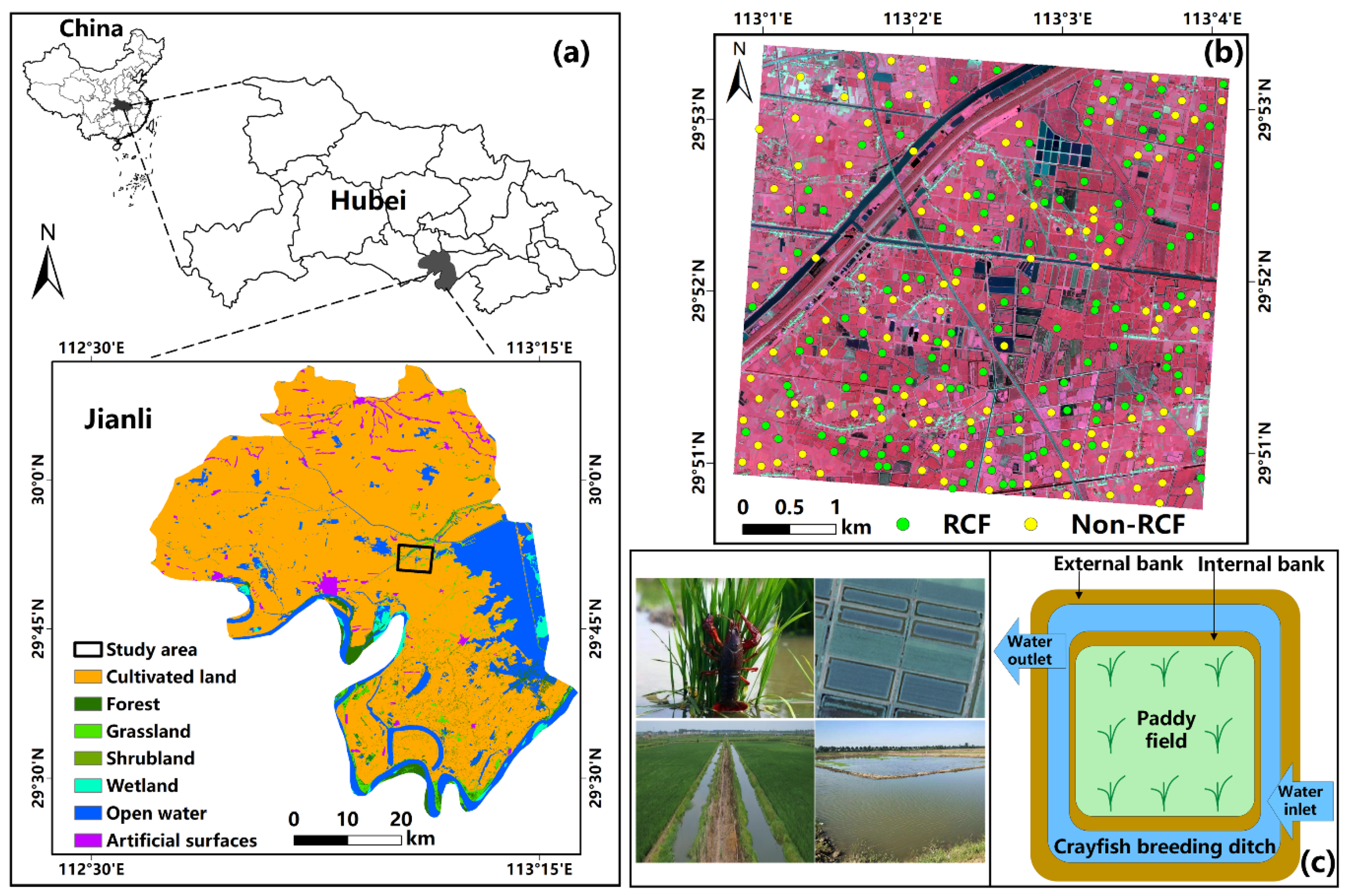
2.1. Study Area

Jianli City, Hubei Province, Central China, is where the study area was located (Figure 1a). Jianli is in a subtropical monsoon climatic zone. The average annual rainfall and temperature in this area are 1200 mm and 16 °C, respectively. Jianli is one of the major food-producing areas in the middle reaches of the Yangtze River. Paddy rice, wheat, corn, oilseed rape, and rice-crayfish are the primary crop types in this city. Among all Chinese counties, Jianli has the largest RCF planting area (approximately 5.3 × 10⁴ ha), accounting for 15% of all RCFs in Hubei Province. According to the availability of high-resolution images of Jianli, we selected a specific region to be the final study area, and the land area of this region was approximately 25 km² (Figure 1). The period of planting rice in an RCF begins in June and harvest occurs in October. In general, farmers put crayfish seeds into ditches in March, and then the crayfish will enter the rice fields for food as they grow up. The adult crayfish are generally harvested twice per year in two time periods, i.e., April to June and August to September.

2.2. Data

We used SuperView-1 images to extract the RCFs in this study. The SuperView-1 constellation, which comprises four satellites (SuperView-1 01, 02, 03 and 04), was designed by China and launched in 2016. The camera onboard the SuperView-1 satellite has four multispectral bands (blue: 450–520 nm, green: 520–590 nm, red: 630–690 nm, and near-infrared (NIR): 770–890 nm) and one panchromatic band (450–890 nm) with a revisit cycle of 1 day [43]. The spatial resolutions of the multispectral bands and panchromatic band are 2 m and 0.5 m, respectively. Two SuperView-1 images acquired on 19 August 2018 (Figure 1b) and 7 April 2019, which refer to the rice growth phase and field flooding phase, respectively, were used in this study. The radiometric and geometric biases of the two images were previously adjusted. We used the Gram-Schmidt algorithm to fuse the multispectral image (2 m) and panchromatic image (0.5 m) into a multispectral image with a 0.5 m resolution to identify the RCFs [24].

A total of 51 RCF samples and 189 samples of other land cover types including 56 cropland, 105 artificial land, 11 water body, and 17 forest samples from field surveys were selected as the training dataset for decision tree classification. The main paddy fields in the study area were RCF, traditional paddy rice, and a small number of lotus root fields. Due to the similar spectral characteristics between traditional paddy rice and lotus root, they were grouped into the “cropland” type. Artificial land consisted of rural buildings and roads. Rivers and ponds were classified as the water bodies. All training samples were carefully selected from pure objects to build the decision tree model. The validation samples were collected from two field surveys in Jianli in September 2018 and May 2019, respectively. Finally, 124 RCF samples and 119 non-RCF samples in 2018 and 110 RCF samples and 95 non-RCF samples in 2019 were respectively used for validating the derived RCF maps.

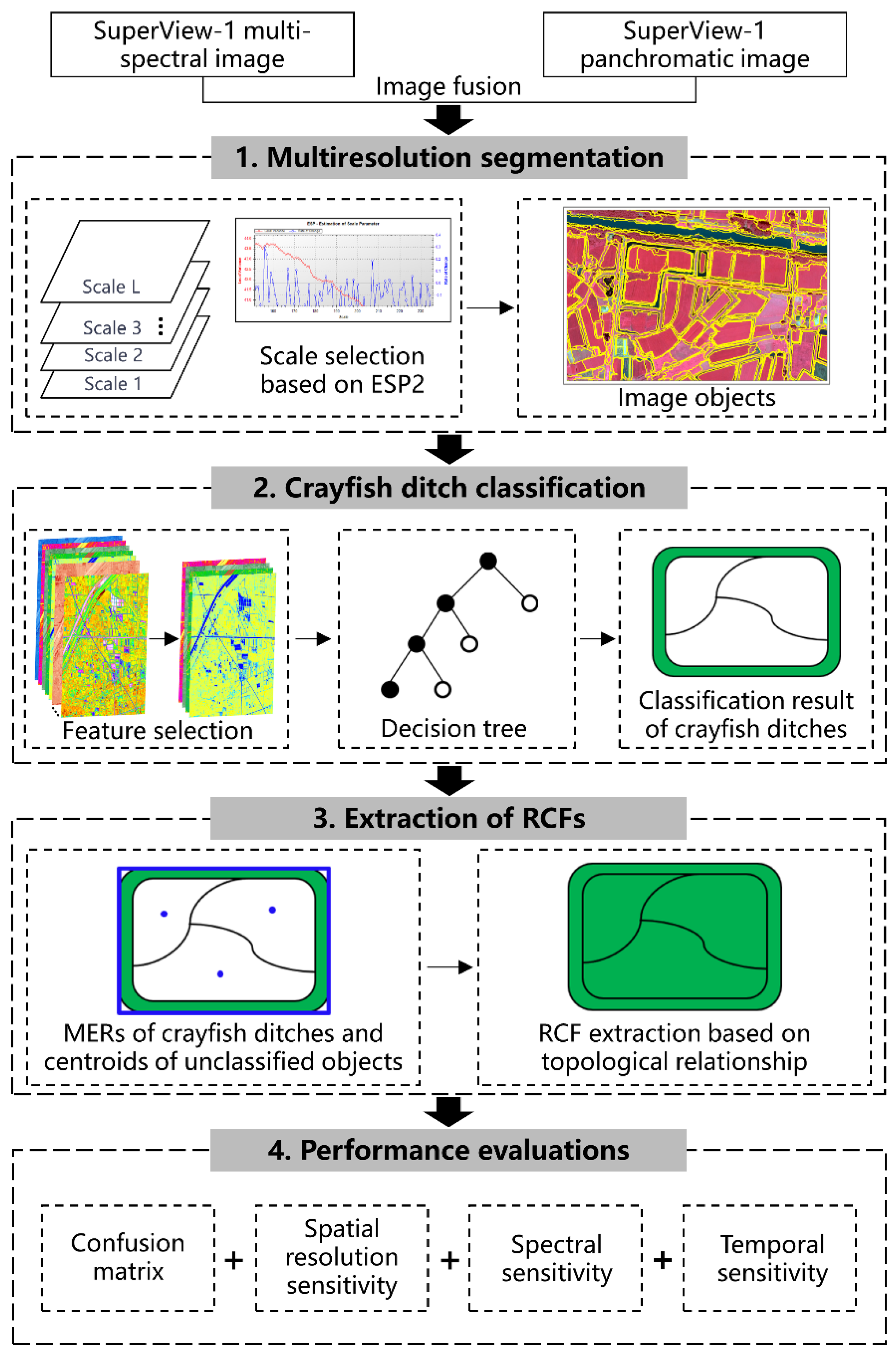
2.3. Framework of the OTBA Method

The OTBA method was proposed to identify RCFs based on their unique crayfish ditch features, and three sequential processes were performed: (1) multiresolution segmentation, (2) crayfish ditch classification, and (3) extraction of RCFs. Figure 2 depicts the OTBA technique flowchart. First, multiresolution segmentation was adopted to obtain crayfish ditch objects. Second, we identified the crayfish ditches using a decision tree model, in which the classification features were selected based on feature separability analysis. Finally, we extracted the RCFs according to the topological relationship between paddy fields and surrounding ditches. A detailed description of each step is provided in Section 2.3.1, Section 2.3.2 and Section 2.3.3.

2.3.1. Multiresolution Segmentation

To create image objects, a multiresolution segmentation method which is embedded in eCognition Developer 9.0 was employed, and it is one of the most widely used object segmentation algorithms [20,44]. A multiresolution segmentation algorithm realizes the purpose of region merging through the bottom-up strategy and is particularly suitable for crop identification using high-resolution images [42]. The algorithm iteratively combines pixels into objects and then merges small and similar objects into larger objects according to the predefined homogeneity criterion [45]. The scale parameter, shape parameter, and compactness parameter are the three important parameters for image segmentation [29]. The shape parameter represents the geometrical characteristics of the objects and the compactness parameter represents the boundary smoothness. The scale parameter needs to be carefully selected since it affects the average size and the internal homogeneity of image objects [46]. Estimation of Scale Parameter 2 (ESP2), an automatic tool, was used to identify the optimal scale parameter to circumvent the time-consuming and subjective trial-and-error technique.

The ESP2 tool evaluates the segmentation effects according to the local variance (LV) as well as its rate of change (ROC) [47]. The ROC was calculated according to Equation (1):

$$ROC=\left[\frac{L{V}_{(L)}-L{V}_{(L-1)}}{L{V}_{(L-1)}}\right]\times 100$$

(1)

where LV_(L) is the LV of objects at the targeted level, and LV_(L−1) is the LV at the next lower level. LV varies with changes in object level, and the ROC curve can illustrate this dynamic change. When the ROC curve presents a local peak value, the corresponding segmentation scale value at this point is potentially optimal [48]. Note that the local peak of ESP2 may be observed at various segmentation scales for different land cover types for one image, resulting in several optimal segmentation scales to be selected [34]. Thus, according to visual inspection of the completeness and boundary consistency of the resultant objects, we carefully selected the optimal segmentation scale for crayfish ditches.

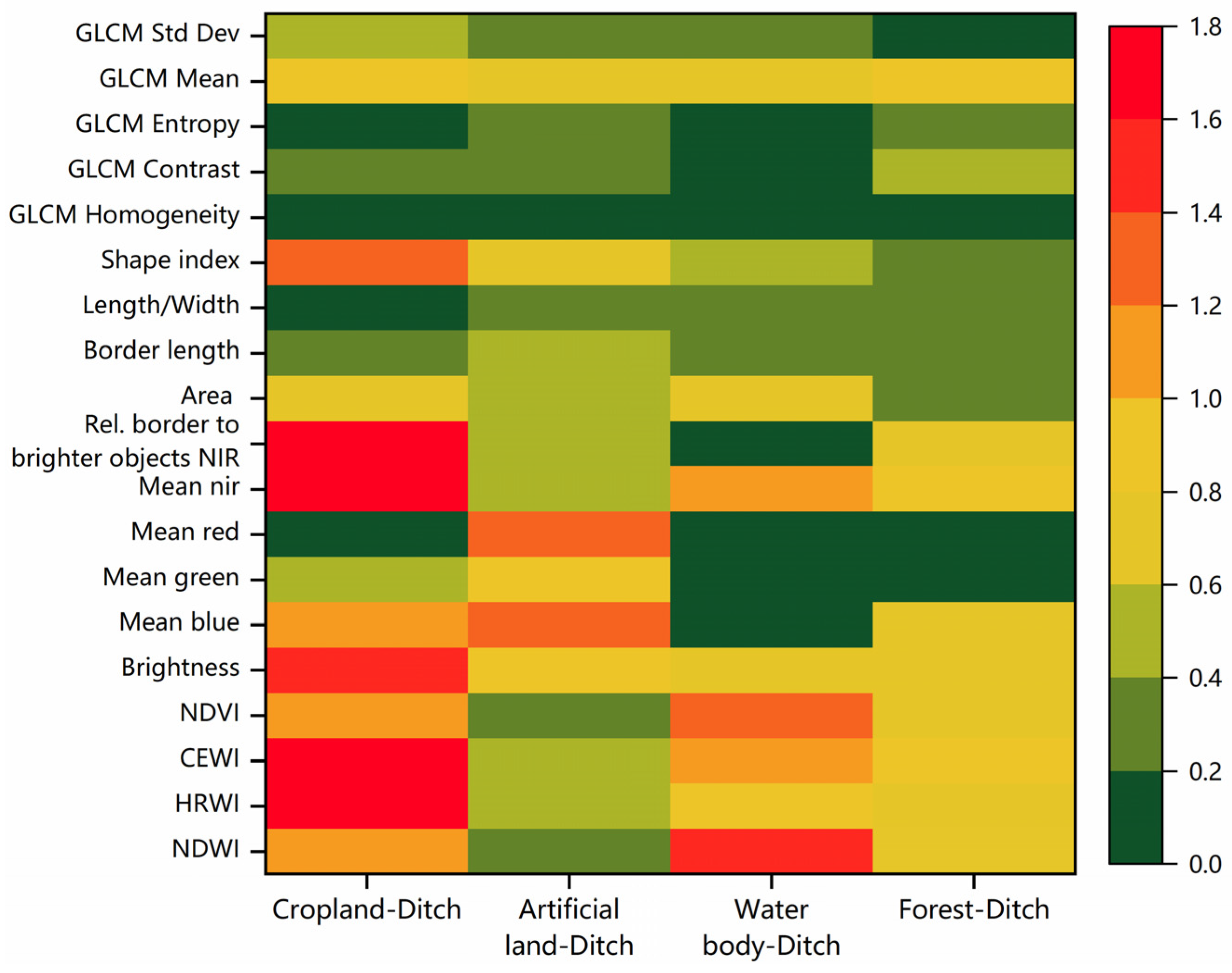
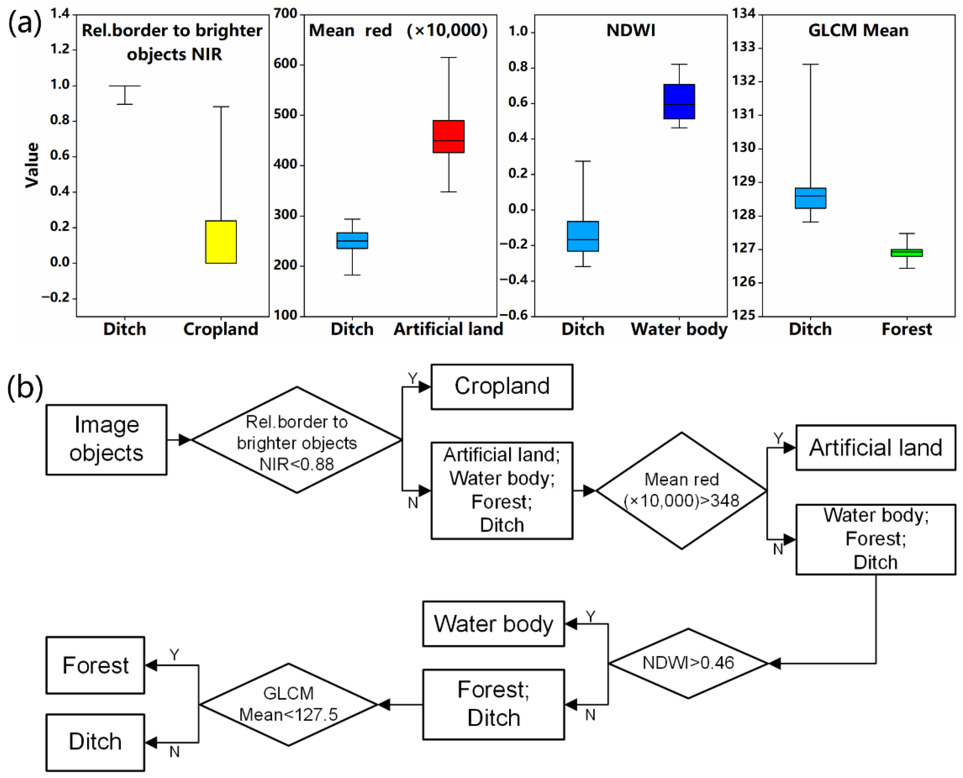
2.3.2. Crayfish Ditch Classification Based on a Decision-Tree Model

A decision-tree classification method was adopted in this work to identify crayfish ditch objects. Decision trees have been widely used in the thematic mapping of crops since they have a flowchart-like structure that is straightforward and easy to interpret [39,42]. In addition to crayfish ditches, the study area mainly included cropland, artificial land, water body, and forest land types. Therefore, we constructed a four-layer decision tree model that aimed to extract crayfish ditch objects by recursively eliminating the abovementioned four other land cover types. The crucial step in building a good decision-tree model is to select the appropriate classification features for different land cover types at tree nodes. In view of the distinctive characteristics of crayfish breeding ditches, such as a narrow width and water information, a total of 19 features (

Table 1. Classification features used in this study.

Feature Category	Selected Features	Equations	Parameters	References
Spectral features	NDWI (Normalized difference water index)	$NDWI=\frac{Green-NIR}{Green+NIR}$	Blue, Green, Red and NIR = surface reflectance values of Blue, Green, Red, NIR bands. #Pv = total number of pixels contained in the object Pv. $c_k(x,y,z,t)$ = the image layer intensity value at pixel $(x,y,z,t)$. $N_v^B$ = the darker direct neighbor to v, with $N_v^B\left\{u\in N_v:{\overline{c}}_k(u)<{\overline{c}}_k(v)\right\}$·$b(v,u)$ = the length of common border between v and u.	[52]
	NDVI (Normalized difference vegetation index)	$NDVI=\frac{NIR-Red}{NIR+Red}$		[53]
	CEWI (Coefficient enhanced water index)	$CEWI=\sqrt{NI{R}^2-2\times (NIR-Blue)}$		[54]
	HRWI (High-resolution water index)	$\begin{array}{ll}HRWI& =6\times Green-Red\\ & +6.5\times NIR+0.2\end{array}$		[55]
	Mean blue, green, red and NIR	${\overline{c}}_k(v)=\frac{1}{\#P_v}{\displaystyle \sum _{(x,y,z,t)\in P_v}{c}_k(x,y,z,t)}$		[56]
	Brightness	$\overline{c}(v)=\frac{1}{4}{\displaystyle \sum _{k=1}^4{\overline{c}}_k(v)}$
	Rel. border to brighter objects NIR	${\displaystyle \sum _{u\in N_v^B}\frac{b(v,u)}{b_v}}$
Geometric features	Border length	$b_v=b_o+b_i$	b0 = the length of outer border. bi = the length of inner border. u = the pixel size in coordinate system units. ${\gamma }_v^{EV}$= the ratio length of v of the eigenvalues. ${\gamma }_v^{BB}$ = the ratio length of v of the bounding box.	[56]
	Area	$A_v=\#P_v\times u^2$
	Length/Width	${\gamma }_v=\min {\gamma }_v^{EV},\max {\gamma }_v^{BB}$
	Shape index	$s_v=\frac{b_v}{4\sqrt{A_v}}$
Textural features	GLCM Entropy	$e_{i,j}={\displaystyle \sum _{i,j=0}^{N-1}{P}_{i,j}}(-\ln P_{i,j})$	i = the row number. j = the column number. $P_{i,j}$ = the normalized value in the cell $i,j$. N = the number of rows or columns.	[56]
	GLCM Mean	${\mu }_{i,j}=\frac{{\displaystyle \sum _{i,j=0}^{N-1}{P}_{i,j}}}{N^2}$
	GLCM Std Dev	${\sigma }_{i,j}=\sqrt{{\displaystyle \sum _{i,j=0}^{N-1}{P}_{i,j}(i,j-{\mu }_{i,j})}}$
	GLCM Homogeneity	$h_{i,j}={\displaystyle \sum _{i,j=0}^{N-1}\frac{P_{i,j}}{1+{(i-j)}^2}}$
	GLCM Contrast	$c_{i,j}={\displaystyle \sum _{i,j=0}^{N-1}{P}_{i,j}}{(i-j)}^2$

) were used as candidate features: (1) 10 spectral features including 4 vegetation indices and 6 spectral band features, (2) 4 geometric features, and (3) 5 textural features. We selected these 19 features because they have been extensively used in object-based classification for agricultural lands [38,49,50] and have shown the potential to reflect the unique spectral and geometric characteristics of RCFs.

With these candidate features, we employed the separability index (SI), which has been demonstrated to be a good indicator to reflect two-class spectral separability [51], to identify the best features for targeted classes. The SI was calculated as follows:

$$S{I}_{di}=\frac{\Delta \mathrm{inter}(d,i)}{\Delta \mathrm{intra}(d,i)}=\frac{\left|\overline{u_d}-\overline{u_i}\right|}{1.96\times ({\sigma }_d+{\sigma }_i)}$$

(2)

where $\overline{u_d}$ and $\overline{u_i}$ are the mean values of a feature of crayfish ditch and land cover type i, respectively, and $\overline{{\sigma }_d}$ and $\overline{{\sigma }_i}$ are the corresponding standard deviations. The $\left|\overline{u_d}-\overline{u_i}\right|$ reflects the interclass heterogeneity, whereas $({\sigma }_d+{\sigma }_i)$ reflects intraclass heterogeneity [51]. Higher interclass heterogeneity and lower intraclass heterogeneity will result in a higher SI, which means that the corresponding features are the optimal features for crayfish ditch classification.

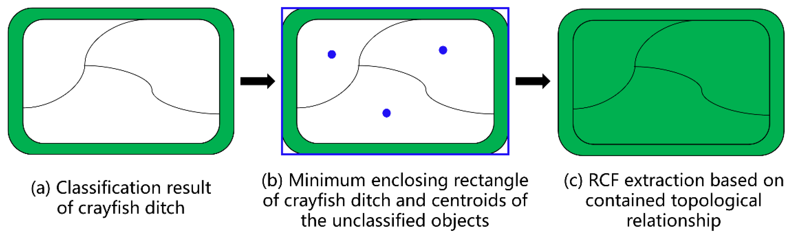
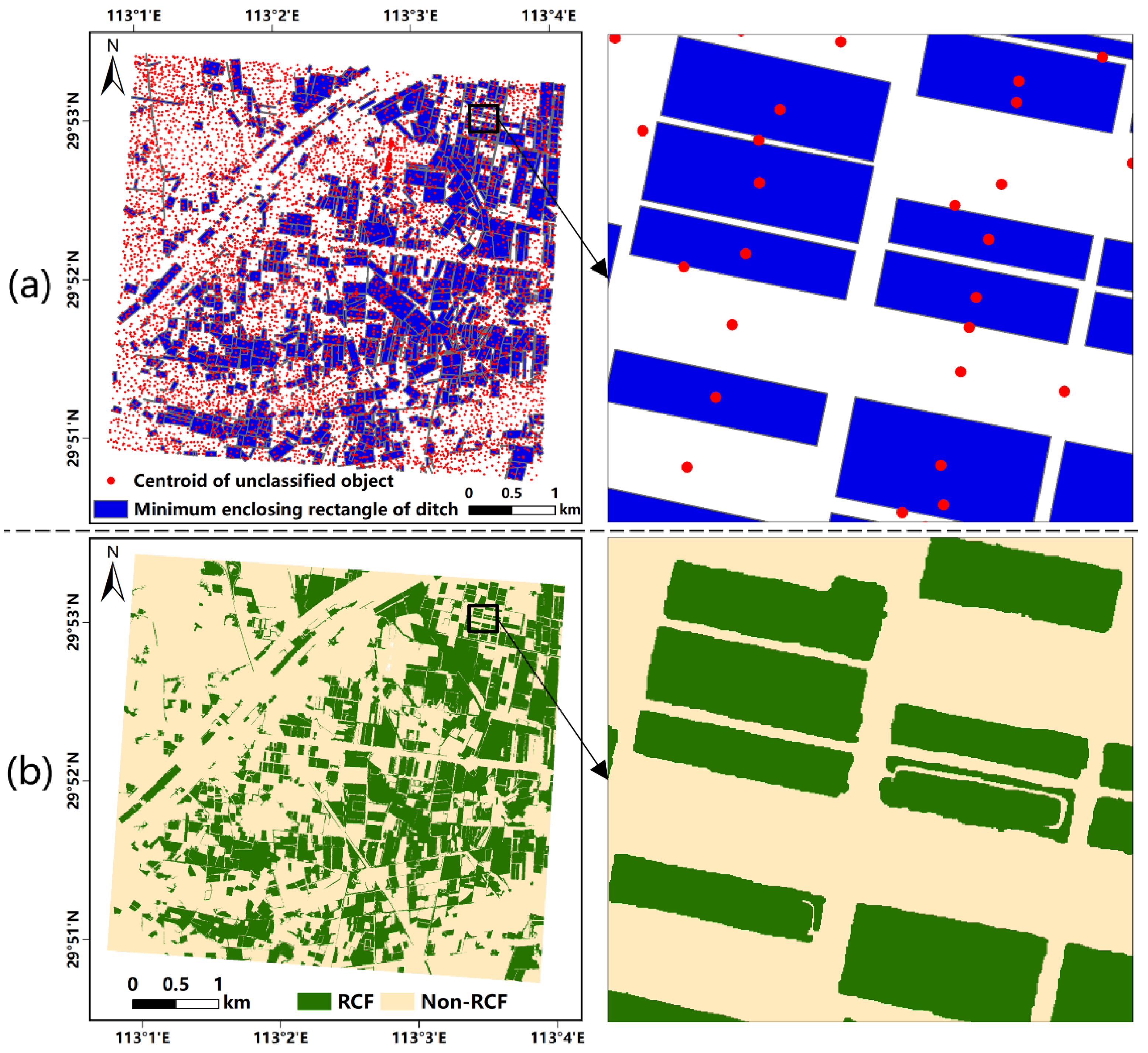
2.3.3. RCF Extraction by Topology

Based on the identified crayfish ditches, the rice fields in the RCF farming system were extracted according to the topological relationship between the crayfish ditches and the adjacent rice fields. The crayfish ditch objects together with the embedded rice field objects comprised the entire RCF. Specifically, we first calculated the centroid of each unclassified object. Then, we estimated the minimum enclosing rectangle of each ditch object, as shown in Figure 3. If the centroids of unclassified objects were located in any of the outer rectangles of the ditches, these undefined objects were grouped into rice fields (Figure 3). Following the above steps, all rice objects were identified from the unclassified objects. Finally, the crayfish ditch objects and rice objects were merged as RCFs.

To further improve the classification results, two post-classification steps were developed. First, since it was inevitable that a crayfish ditch may be segmented into multiple objects in the segmentation process, which might reduce the integrity of the resultant RCFs, we obtained the entire crayfish ditch by merging contiguous ditch objects. Second, we removed the misclassified ditch from the crayfish ditch classification result when the outer rectangle of a ditch did not contain any other object’s centroid.

2.4. Performance Evaluations

To evaluate the RCF classification performances of the OTBA method, we collected a total of 243 field samples. The traditional error matrix and its adjunctive indicators, including the overall accuracy, user’s accuracy and producer’s accuracy, were adopted to assess the classification accuracy.

Since the OTBA was developed to extract RCFs mainly according to the geometrical features of crayfish ditches, which were characterized by a high spatial resolution image, we assessed how spatial resolution impacted on RCF classification performance. To do so, we resampled the original 0.5 m image to different resolutions (i.e., 1 m, 2 m, 3 m, 5 m, 8 m and 10 m) and implemented OTBA classification and validation. In addition, to determine the lower limit of the spatial resolution for RCF mapping, we adopted the Z-test to quantitatively assess the significance in differences of RCF classifications from images with different spatial resolutions. The Z-test can be expressed as the Equation (3) [57]:

$$Z=\frac{\frac{X_1}{N_1}-\frac{X_2}{N_2}}{\sqrt{\rho (1-\rho )(\frac{1}{N_1}+\frac{1}{N_2})}}$$

(3)

where N₁ and N₂ represent the sizes of sample sets used in two different classifications, X₁ and X₂ refer to the quantities of samples which are rightly classified, and ρ can be derived from (X₁ + X₂)/(N₁ + N₂). There exists a significant difference between the two classifications if the |Z| value is greater than or equal to 1.96, which is estimated at the widely used 5% significance level.

In addition to the spatial resolution, we assessed the sensitivity of the OTBA approach to spectral bands. Therefore, we compared the classification results derived from the original image with four (i.e., red, green, blue, and NIR) spectral bands and the image with only three (i.e., red, green, and blue) bands. Moreover, to evaluate how the temporal information affected the OTBA method, we compared the classification results derived from the image in the rice growth phase when the field was covered by rice (Figure 1c) and the image in the flooding phase when the field was mainly covered by water (Figure 1c).

3. Results

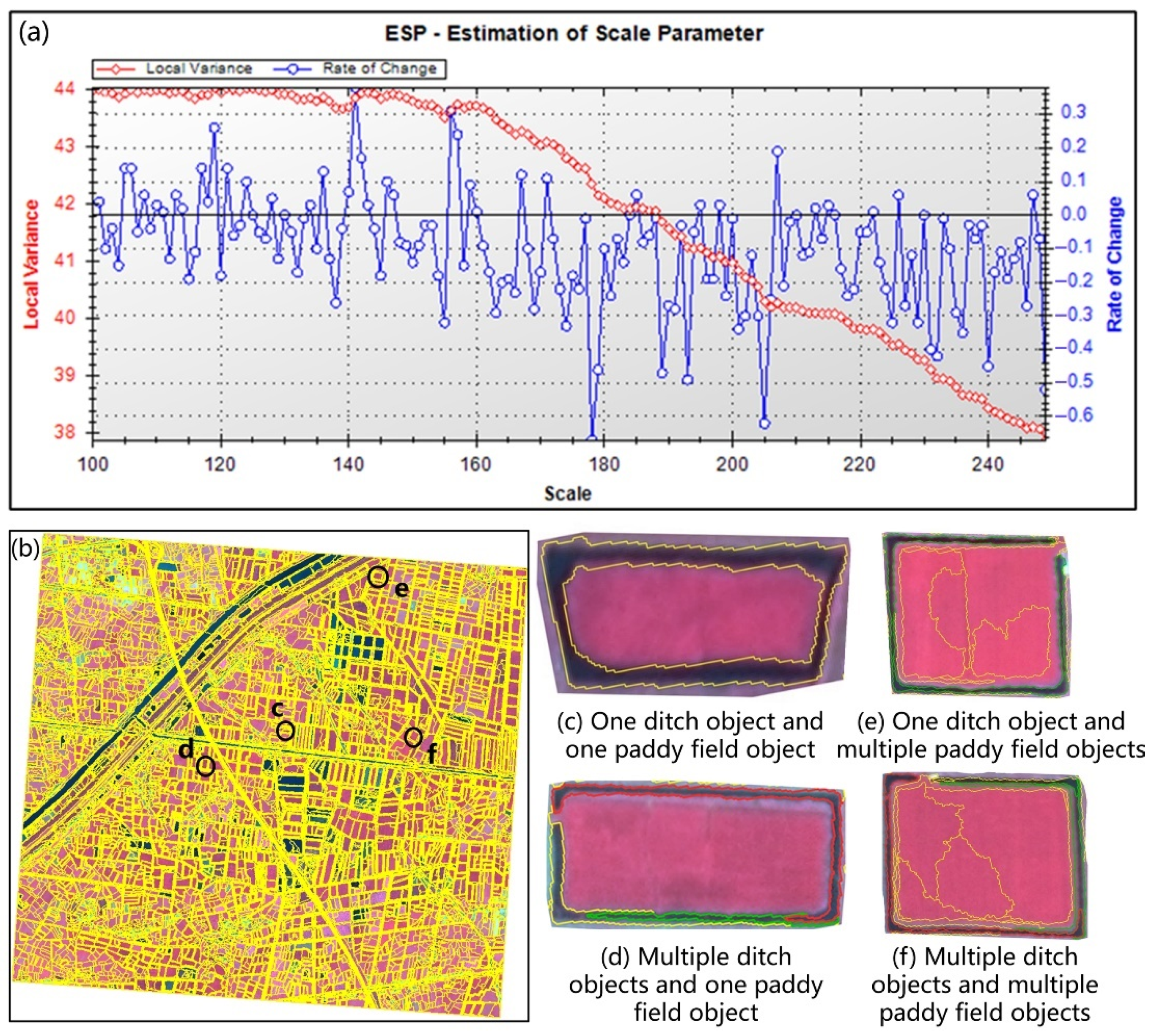
3.1. Optimal Scale Parameter and Image Segmentation Result

The ideal scale parameter and image objects obtained from the multiresolution segmentation method based on the ESP2 tool are shown in Figure 4. We observed that the local variance decreased with increasing segmentation scale. Furthermore, when the scale changed, the rate of change of local variance fluctuated significantly for the reason that the heterogeneity of image objects generated by different scales may vary greatly. There were four local peaks, i.e., 119, 141, 156 and 207, for the ROC curve, which represented the potential optimal segmentation scales for crayfish ditches. According to the visual judgments of segmentation objects, we selected 207 as the optimal scale parameter, at which the completeness and boundary consistency of crayfish ditch objects were the best. After several trial-and-error tests, the shape parameter and the compactness parameter were finally adjusted to 0.7 and 0.2. As a result, a total of 10364 image objects were generated for this area.

As shown in Figure 4, there were generally four patterns of image objects for an RCF: (1) a crayfish ditch object and a paddy field object, (2) multiple crayfish ditch objects and a paddy field object, (3) a crayfish ditch object and multiple paddy field objects, and (4) multiple crayfish ditch objects and multiple paddy field objects. According to the strategy described in Section 2.3, we merged the contiguous multiple ditch objects into a circular crayfish ditch with high integrity.

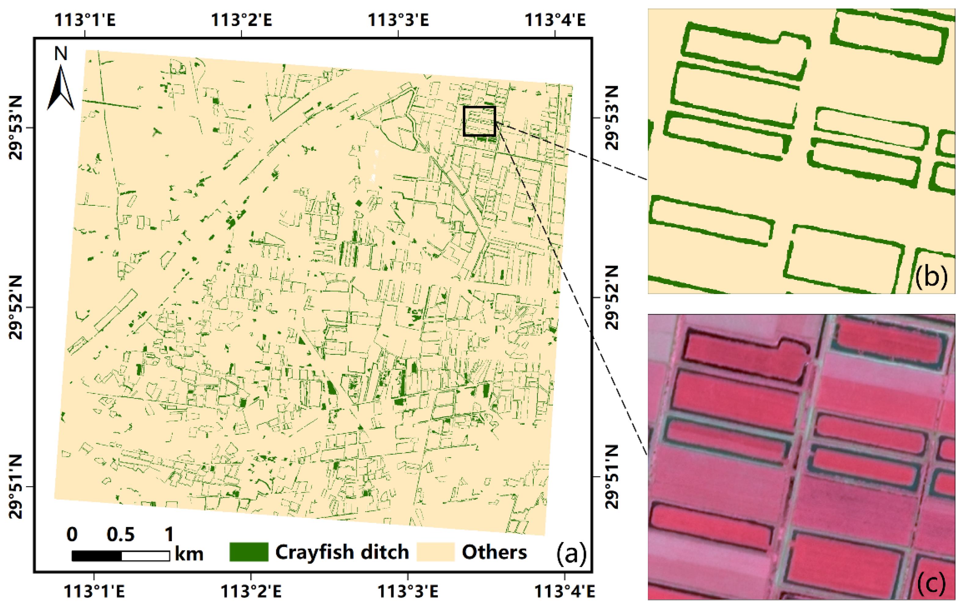
3.2. Classification Model and Result of Crayfish Ditch

Figure 5 presents the separability chart of four pairwise classes for the 19 features. A high SI value indicates high separability between the two classes for a given feature. The highest SI of 1.72 was observed for cropland and ditches at the feature Rel. border to brighter objects NIR, indicating that ditches were most easily distinguished from cropland by using this feature. The feature Rel. border to brighter objects NIR reflected how much the perimeter of an object was surrounded by objects with higher near-infrared reflectance. The reason for this observation was that the near-infrared reflectance of crayfish ditches in the flooding state that were mainly covered by water was much lower than that of the surrounding rice field, resulting in a higher Rel. border to brighter objects NIR of a ditch than that of a paddy field. The Mean red, with an SI value of 1.24, performed better than the other features in terms of separating artificial land and ditches. For water body and ditches, the NDWI was the best feature for distinguishing them, and it had an SI value of 1.44. Due to abundant vegetation around the ditch (Figure 1c), the near-infrared reflectance of the crayfish ditch was higher than that of the water body, leading to a much smaller NDWI for the crayfish ditch. Among all features, the textural feature GLCM Mean presented the highest SI for separating ditches from forests. Thus, the decision tree classification model was built by setting these features with the highest SI values as the final classification features.

To determine the thresholds for the selected features of the decision-tree model, we estimated the value ranges of these features for different pairwise classes (Figure 6a). The feature Rel. border to brighter objects NIR was less than 0.88 for cropland, while the minimum value of crayfish ditches was 0.90. Therefore, the threshold of Rel. border to brighter objects NIR was set to 0.88 to distinguish between cropland and ditches. The minimum of Mean red (multiplied by 10,000) was 348 for artificial land, and the value was less than 294 for ditches. The NDWI of all ditch objects was less than 0.27, which was significantly less than the minimum NDWI (i.e., 0.46) of water body objects. It was also observed that the marginal value of GLCM Mean to separate ditches from forests was 127.5. With these optimal features and associated thresholds, the decision tree used to extract the crayfish ditches can be developed, as shown in Figure 6b.

The crayfish ditches were then identified using the above decision-tree classification model (Figure 7a). We found that most ditches were circular and relatively enclosed. Although a small number of road objects and river objects were misclassified into crayfish ditches, the classification performance of ditches was generally satisfactory, based on a visual comparison with the original SuperView-1 image.

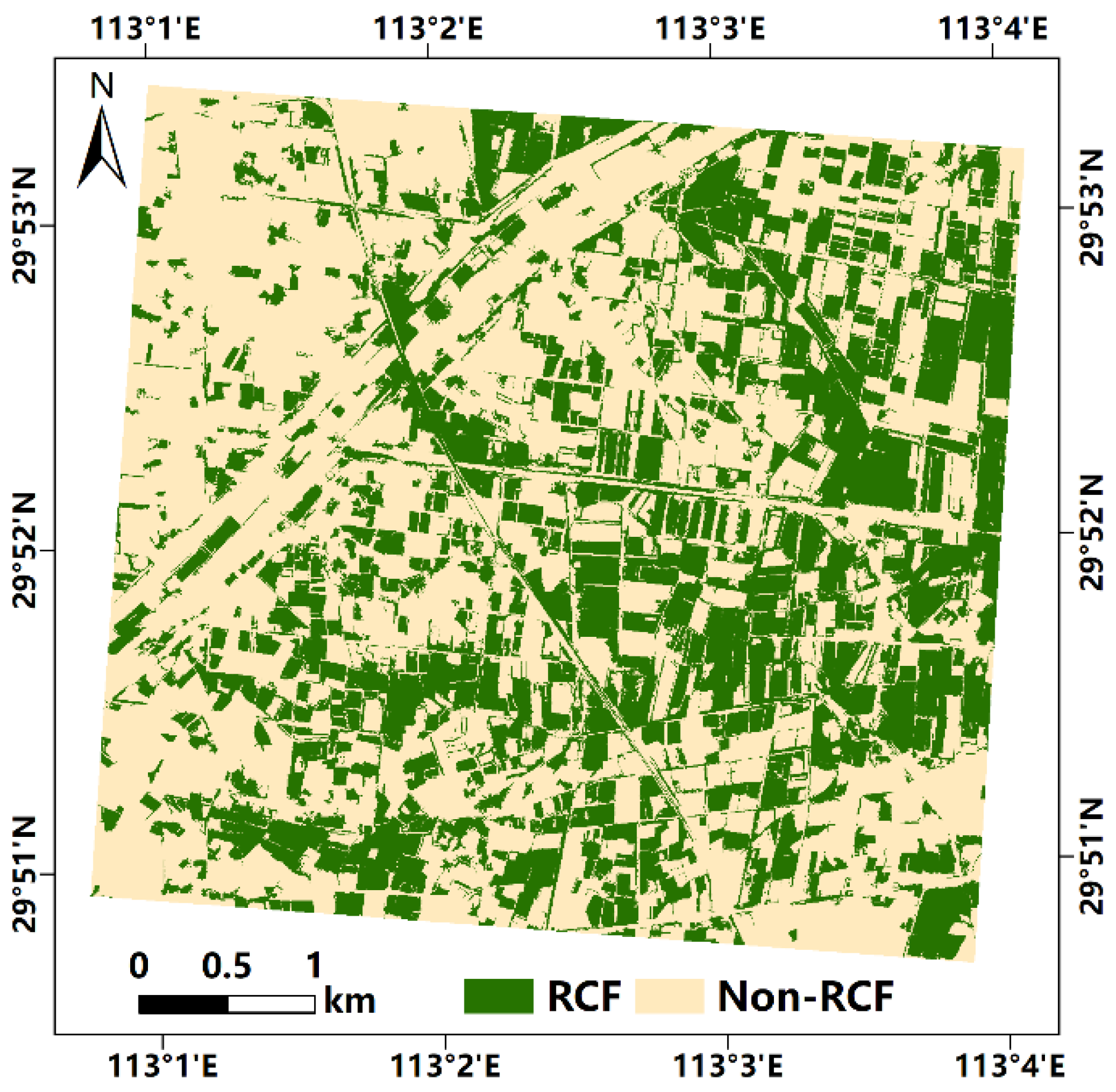
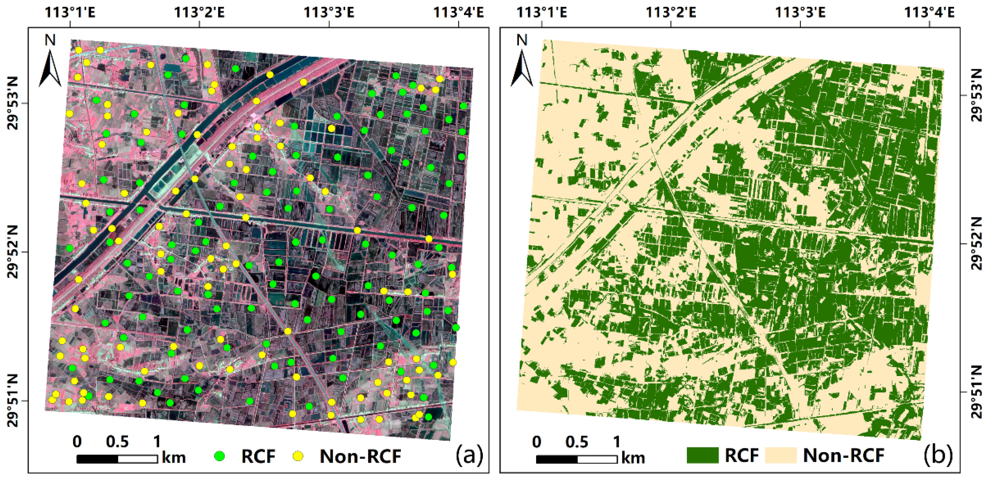
3.3. RCF Map and Accuracy Assessment

With the classification results of the crayfish ditch, an RCF was extracted according to the topological relationship between the crayfish ditch and its neighboring paddy rice (Figure 8). Specifically, the minimum enclosing rectangles of ditch objects and the centroids of unclassified objects are shown in Figure 8a. Figure 8b presents the map of the RCFs in the study area, and the RCFs were composed of crayfish ditches and paddy rice. The overall classification accuracy of RCFs was 91.77% by using the OTBA method and the 0.5 m SuperView-1 image on 19 August 2018 (

Table 2. The evaluation of derived RCF map using the field samples.

Class	RCF	Non-RCF	Total	Producer’s Accuracy
RCF	112	12	124	90.32%
Non-RCF	8	111	119	93.28%
Total	120	123	243
User’s Accuracy	93.33%	90.24%
Overall Accuracy	91.77%

). The producer’s accuracy for RCFs was 90.32% and the corresponding user’s accuracy was 93.33%, indicating the good performance of the OTBA method for extracting RCFs. In addition, our results showed that the area of RCFs in 2018 was 822 ha in the study area.

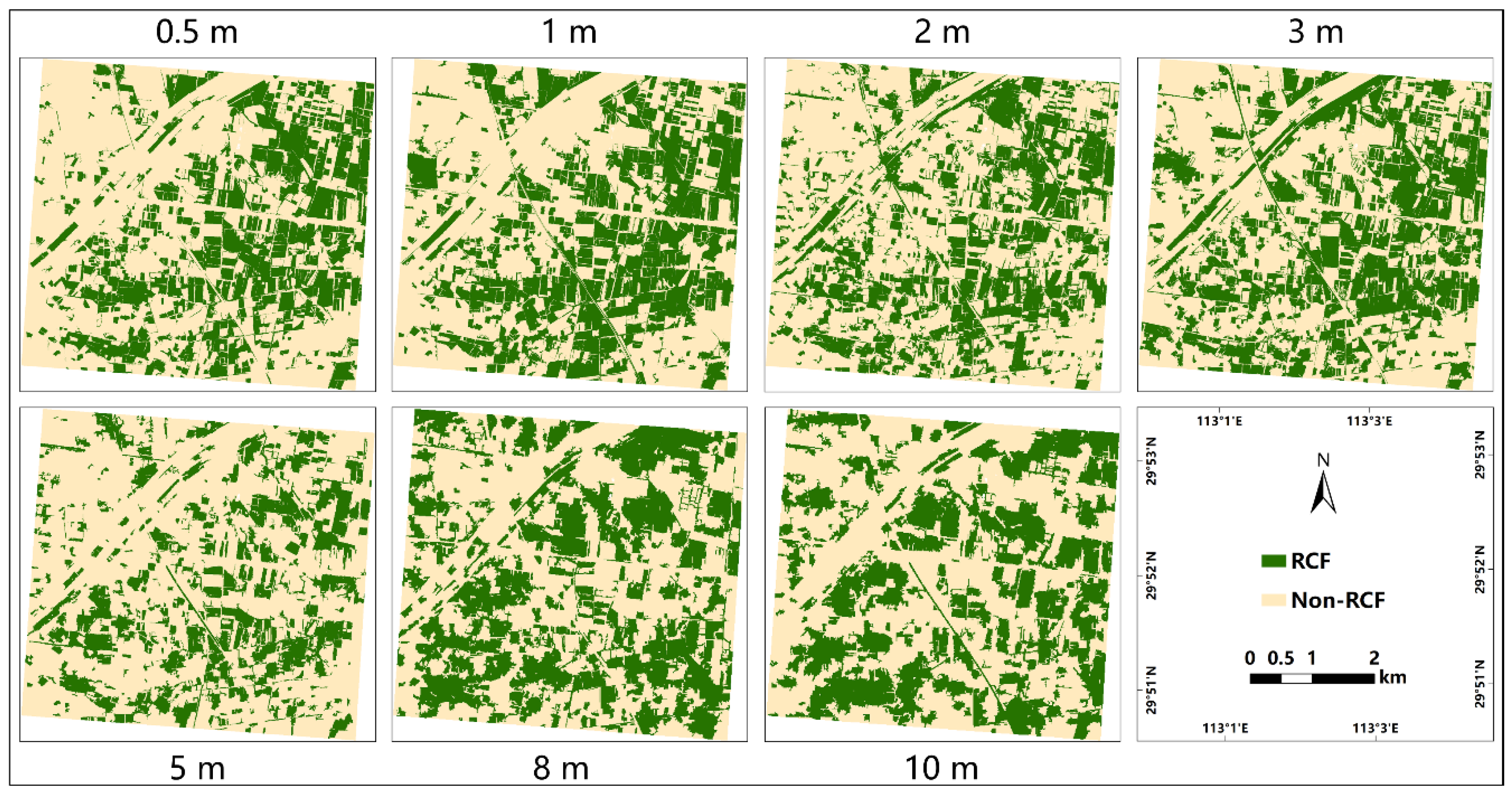
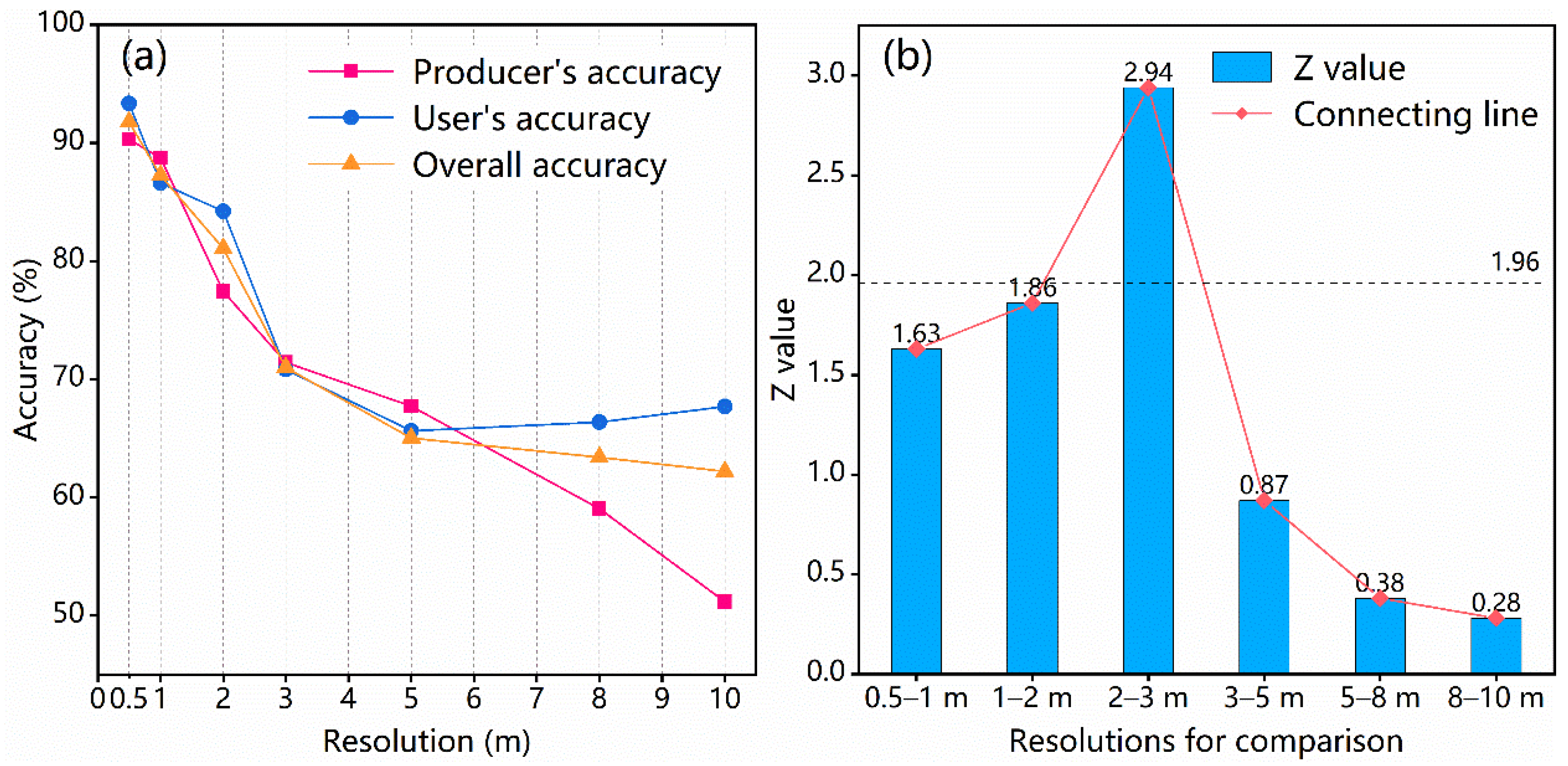
3.4. RCF Mapping Based on Different Spatial, Spectral and Temporal Information

Figure 9 and Figure 10 show the RCF maps and corresponding classification accuracies based on images with different spatial resolutions (i.e., 0.5 m, 1 m, 2 m, 3 m, 5 m, 8 m and 10 m). We observed that all classification accuracies, including the user’s accuracy, producer’s accuracy and overall accuracy of RCFs, decreased with spatial resolution as expected. The accuracies of the RCF map based on images of 1 m resolution were greater than 85%. However, when the spatial resolution decreased to 2 m, the accuracies of the RCF maps, particularly the producer’s accuracy, dropped below 80%. According to the Z-test statistics, the difference in RCF classification accuracies between 0.5 m and 1 m or between 1 m and 2 m was not significant, with all Z values of less than 1.96 at the 95% test level. However, the Z value between 2 m and 3 m was 2.94, indicating a significant difference in their classification results.

Additionally, the NIR band was excluded to analyze the impacts of different spectral bands for identifying RCFs. It should be noted that we adjusted the candidate features for crayfish ditch extraction (Table S1 in the Supplementary Material) due to the lack of an NIR band. The RCF map and associated classification accuracies derived by using the RGB image are shown in Figure 11 and Table S2 (Supplementary Material). Compared with the classification accuracies of using the original four spectral bands, the overall accuracy, user’s accuracy, and producer’s accuracy without using the NIR band decreased by 10%, 9% and 15%, respectively.

To understand the OTBA performance for RCF mapping in different observation dates, the RCF extraction result based on the image from 7 April 2019 in the rice field flooding phase was generated (Figure 12b). Compared with the RCF area (i.e., 822 ha) in 2018, the RCF area (i.e., 1085 ha) in 2019 was significantly increased, which was consistent with the fact that the RCF area expanded rapidly between 2018 and 2019. The user’s and producer’s accuracies and overall accuracy of RCF extraction in the field flooding stage were 4%, 6% and 6% lower than those in the rice growth stage, respectively (Table S3 in Supplementary Material).

4. Discussion

4.1. The Sensitivity of Spatial, Spectral and Temporal Information on the OTBA Method

With the very high-resolution image of 0.5 m (i.e., SuperView-1), we well characterized the topological relationship between crayfish ditches and paddy fields to accurately identify RCFs. However, images with a 0.5 m spatial resolution are not always available, and mapping RCFs in a large region with satellite images of less than 1 m often requires high costs. To evaluate the generalization of the OTBA method to different satellite images, we investigated the lower limit of image spatial resolution that could achieve satisfactory RCF classification accuracies (described in Section 2.4). Based on the performance of derived RCF maps, we found that the classification result presented significant differences when the spatial resolution decreased to 2 m (Figure 10). Therefore, the lower limit of the image resolution for mapping RCFs with high reliability (overall accuracy = 81.07%) based on the OTBA method was 2 m, indicating the good generalization capability of the OTBA method. Additionally, these results provide important references for the selection of appropriate images for mapping RCFs over large regions.

The OTBA method mainly took advantage of spatial features and topological relationships among land cover types to identify RCFs, which raised the question of whether the OTBA method requires rich spectral bands. The results in Figure 11 show significant declines in several accuracy indicators, suggesting that the NIR band is a very important feature that cannot be ignored for the OTBA method. Furthermore, the decreased accuracies using the RGB image was explained by the fact that the optimal crayfish ditch classification features, including Rel. border to brighter objects NIR (to eliminate cropland objects) and NDWI (to eliminate water body objects), which are both related to the NIR band, were excluded in this case. Although the RGB image can be used to produce an RCF map with acceptable accuracy (overall accuracy = 80.49%), an image with NIR band information is recommended to further improve the performance of the OTBA method.

In addition, there were two important phases for cultivating RCFs: one was the field flooding stage (the end of October to May of the next year) when the field was mainly covered by water, and the other was the rice growth stage (June to October) when the field was mainly covered by rice. The SuperView-1 image used in this study was in the rice growth phase (i.e., 19 August 2018), with which we achieved satisfactory RCF mapping results. However, very high-resolution images are not always available in every phase of crop farming, particularly in South China, where cloudy and rainy weather is frequent. Therefore, to evaluate the impact of temporal information of satellite images on the OTBA method, we added the experiment using the image obtained in the field flooding phase for RCF classification. Results showed classification accuracies based on the images in flooding phase were lower than those in rice growth phase (Figure 12). Such results can be explained by that the spectral signature of RCFs in the flooding stage was influenced by a mixture of water and other impurities (e.g., straw and waterweeds), leading to the increased probability of class confusion. Therefore, high-resolution images in the rice growth stage from June to October are preferred for mapping RCFs. However, regardless of the relatively low mapping accuracy in comparison with that in the rice growth period, the RCFs in the rice flooding stage achieved an overall accuracy of 85.85%, which is generally satisfactory for most agricultural applications.

4.2. Advantages and Further Improvements

Previous studies have shown that mapping rice is challenging because it is difficult to capture the key phenological phase, and rice is easily misclassified with other crop types [16,18,58]. For example, He et al. [59] claimed that the proportion of valid observations in key phenological phases of paddy rice was less than 60% in their study area, resulting in extremely poor accuracy of early rice identification. Zhou et al. [60] and Zhang et al. [15] pointed out that rice was very easy to be mixed with wetland or edge pixels of rivers and lakes. In order to eliminate the interference of the abovementioned land cover types, they introduced existing land cover classification datasets or established many additional classification rules to improve the classification accuracy. RCFs, which are composed of not only rice fields but also crayfish ditches, display higher intraclass spectral variance than traditional rice patterns do. Therefore, identifying entire RCFs based on the common strategy that relies solely on the spectral signature of land cover classes tends to be difficult. Considering the specific characteristic of RCFs, our proposed OTBA method first identified the crayfish ditches of RCFs using spectral and spatial features based on a decision-tree model and then extracted rice fields of RCFs using the topological relationships between crayfish ditches and rice fields. In this way, the OTBA method does not need to identify rice, which to a large extent avoids addressing the complex spectral heterogeneity of rice fields and therefore can improve the performance of the OTBA method effectively for extracting whole RCFs.

Furthermore, an accurate extraction of crayfish ditch is crucial for the OTBA method. A large number of studies mainly used pixel-based methods and relied on spectral features (e.g., spectral bands and water indices) to extract water bodies [61,62,63]. However, the ‘salt and pepper effect’ [35] existing in the pixel-based process will significantly affect the extraction accuracy and integrity of small water bodies such as crayfish ditches. Huang et al. [64] extracted multi-class urban water bodies (including rivers, lakes, small ponds, and narrow canals) using spectral indices and machine learning, but they found that the extraction performance at pixel level was inferior, with obvious omission and commission errors. In addition, identifying water body only based on spectral features has great uncertainty. For example, Wang et al. [65] used a water index to extract water, which showed serious cases of misclassifying building shadows (sharing similar index value with water) as water and missing small water bodies (mixed with other objects). By contrast, we employed an object-based method, which ingested not only spectral signatures but also spatial signatures and neighborhood relationships, to extract crayfish ditches. The good accuracy and high completeness of the extracted crayfish ditch are essential for the improvement of RCF mapping. It is noteworthy that although we developed the OTBA method to map RCFs in Jianli City using SuperView-1 images, the OTBA can be easily generalized to other regions even with fragmented landscapes and other high-resolution images with spatial resolutions of higher than 2 m.

Additionally, two major improvements could be made when extending the OTBA method for RCF identification in a larger area. First, most of the RCFs in this study were rectangular, but a few RCFs were convex or concave. These nonrectangular RCFs could increase the commission errors if using the minimum enclosing rectangle to characterize the topological relationships between rice fields and crayfish ditches. More approaches, such as the area filling method and other minimum enclosing polygons, will be tested to extract RCFs with various shapes in future work. Second, since it is generally difficult to cover a large area with single-source satellite data, considerable efforts should be made to collect and integrate multisource high spatial resolution images for large-region RCF mapping.

5. Conclusions

In this work, we presented an OTBA method to map RCFs, which are an increasingly popular farming pattern used in South China. The OTBA method first identified the crayfish ditches using an object-based decision tree method and then extracted the paddy field objects using the topological relationship between the ditches and paddy fields. The final RCF was a combination of the ditch and paddy field objects. Jianli City, which has the largest planting area of RCFs in Hubei Province, was chosen as the research site for evaluating the OTBA method. In addition, we carefully explored the impacts of various spatial resolutions, spectral bands, and temporal information on RCF mapping. Our results showed that the overall accuracy, user’s accuracy, and producer’s accuracy of the derived RCF map were 91.77%, 93.33% and 90.32%, respectively, indicating that the proposed OTBA method performed well. The mapping accuracy of RCFs gradually decreased with decreasing image spatial resolution, as expected. Nevertheless, the OTBA method can generate satisfactory mapping results for RCFs as long as the spatial resolution is greater than 2 m. The NIR band, which was used to calculate crucial spectral features (i.e., Rel. border to brighter objects NIR and NDWI) for identifying crayfish ditches, plays an important role in accurately mapping RCFs. Moreover, high-resolution images in the rice growth stage performed better than those in the flooding stage for mapping RCFs, with a 5% accuracy gap, providing a good reference for the selection of images on a specific observation date. Our proposed method fully utilized the spectral features, spatial features and neighborhood relationships among land use objects to identify whole RCFs, which largely reduced the uncertainty of the high intraclass spectral variance associated with paddy rice. The OTBA method can be easily generalized to other study areas regardless of fragmented agricultural landscapes and other high-resolution (≤2 m) images. Furthermore, since a single satellite that produces high-resolution images suffers from the long revisit cycle, integrating multisource high-resolution images is an important direction for large-region RCF mapping in the future.

References

1. Wang, Y.; Wang, C.; Chen, Y.; Zhang, D.; Zhao, M.; Li, H.; Guo, P. Microbiome Analysis Reveals Microecological Balance in the Emerging Rice-Crayfish Integrated Breeding Mode. Front. Microbiol. 2021, 12, 669570. [Google Scholar] [CrossRef]
2. Yu, J.; Ren, Y.; Xu, T.; Li, W.; Xiong, M.; Zhang, T.; Li, Z.; Liu, J. Physicochemical water quality parameters in typical rice-crayfish integrated systems (RCIS) in China. Int. J. Agric. Biol. Eng. 2018, 11, 54–60. [Google Scholar] [CrossRef] [Green Version]
3. Liu, C.; Hu, N.; Song, W.; Chen, Q.; Zhu, L. Aquaculture Feeds Can Be Outlaws for Eutrophication When Hidden in Rice Fields? A Case Study in Qianjiang, China. Int. J. Environ. Res. Public Health 2019, 16, 4471. [Google Scholar] [CrossRef] [Green Version]
4. Sun, Z.; Guo, Y.; Li, C.; Cao, C.; Yuan, P.; Zou, F.; Wang, J.; Jia, P.; Wang, J. Effects of straw returning and feeding on greenhouse gas emissions from integrated rice-crayfish farming in Jianghan Plain, China. Environ. Sci. Pollut. Res. 2019, 26, 11710–11718. [Google Scholar] [CrossRef] [PubMed]
5. Hou, J.; Styles, D.; Cao, Y.; Ye, X. The sustainability of rice-crayfish coculture systems: A mini review of evidence from Jianghan plain in China. J. Sci. Food Agric. 2021, 101, 3843–3853. [Google Scholar] [CrossRef] [PubMed]
6. Li, Q.; Xu, L.; Xu, L.; Qian, Y.; Jiao, Y.; Bi, Y.; Zhang, T.; Zhang, W.; Liu, Y. Influence of consecutive integrated rice-crayfish culture on phosphorus fertility of paddy soils. Land Degrad. Dev. 2018, 29, 3413–3422. [Google Scholar] [CrossRef]
7. Si, G.H.; Peng, C.L.; Yuan, J.F.; Xu, X.Y.; Zhao, S.J.; Xu, D.B.; Wu, J.S. Changes in soil microbial community composition and organic carbon fractions in an integrated rice-crayfish farming system in subtropical China. Sci. Rep. 2017, 7, 2856. [Google Scholar] [CrossRef]
8. Hu, Q.; Yin, H.; Friedl, M.A.; You, L.; Li, Z.; Tang, H.; Wu, W. Integrating coarse-resolution images and agricultural statistics to generate sub-pixel crop type maps and reconciled area estimates. Remote Sens. Environ. 2021, 258, 112365. [Google Scholar] [CrossRef]
9. Kluger, D.M.; Wang, S.; Lobell, D.B. Two shifts for crop mapping: Leveraging aggregate crop statistics to improve satellite-based maps in new regions. Remote Sens. Environ. 2021, 262, 112488. [Google Scholar] [CrossRef]
10. Yan, L.; Roy, D.P. Conterminous United States crop field size quantification from multi-temporal Landsat data. Remote Sens. Environ. 2016, 172, 67–86. [Google Scholar] [CrossRef] [Green Version]
11. Burke, M.; Driscoll, A.; Lobell, D.B.; Ermon, S. Using satellite imagery to understand and promote sustainable development. Science 2021, 371, eabe8628. [Google Scholar] [CrossRef]
12. Weiss, M.; Jacob, F.; Duveiller, G. Remote sensing for agricultural applications: A meta-review. Remote Sens. Environ. 2020, 236, 111402. [Google Scholar] [CrossRef]
13. Xie, Y.; Lark, T.J. Mapping annual irrigation from Landsat imagery and environmental variables across the conterminous United States. Remote Sens. Environ. 2021, 260, 112445. [Google Scholar] [CrossRef]
14. Xiao, X.; Boles, S.; Frolking, S.; Li, C.; Babu, J.Y.; Salas, W.; Moore, B. Mapping paddy rice agriculture in South and Southeast Asia using multi-temporal MODIS images. Remote Sens. Environ. 2005, 100, 95–113. [Google Scholar] [CrossRef]
15. Zhang, G.; Xiao, X.; Dong, J.; Kou, W.; Jin, C.; Qin, Y.; Zhou, Y.; Wang, J.; Menarguez, M.A.; Biradar, C. Mapping paddy rice planting areas through time series analysis of MODIS land surface temperature and vegetation index data. ISPRS J. Photogramm. Remote Sens. 2015, 106, 157–171. [Google Scholar] [CrossRef] [PubMed] [Green Version]
16. Dong, J.; Xiao, X. Evolution of regional to global paddy rice mapping methods: A review. ISPRS J. Photogramm. Remote Sens. 2016, 119, 214–227. [Google Scholar] [CrossRef] [Green Version]
17. Zhang, G.; Xiao, X.; Biradar, C.M.; Dong, J.; Qin, Y.; Menarguez, M.A.; Zhou, Y.; Zhang, Y.; Jin, C.; Wang, J.; et al. Spatiotemporal patterns of paddy rice croplands in China and India from 2000 to 2015. Sci. Total Environ. 2017, 579, 82–92. [Google Scholar] [CrossRef] [PubMed]
18. Qin, Y.; Xiao, X.; Dong, J.; Zhou, Y.; Zhu, Z.; Zhang, G.; Du, G.; Jin, C.; Kou, W.; Wang, J.; et al. Mapping paddy rice planting area in cold temperate climate region through analysis of time series Landsat 8 (OLI), Landsat 7 (ETM+) and MODIS imagery. ISPRS J. Photogramm. Remote Sens. 2015, 105, 220–233. [Google Scholar] [CrossRef] [Green Version]
19. Ding, M.; Guan, Q.; Li, L.; Zhang, H.; Liu, C.; Zhang, L. Phenology-Based Rice Paddy Mapping Using Multi-Source Satellite Imagery and a Fusion Algorithm Applied to the Poyang Lake Plain, Southern China. Remote Sens. 2020, 12, 1022. [Google Scholar] [CrossRef] [Green Version]
20. Belgiu, M.; Csillik, O. Sentinel-2 cropland mapping using pixel-based and object-based time-weighted dynamic time warping analysis. Remote Sens. Environ. 2018, 204, 509–523. [Google Scholar] [CrossRef]
21. Blaschke, T.; Hay, G.J.; Kelly, M.; Lang, S.; Hofmann, P.; Addink, E.; Feitosa, R.Q.; van der Meer, F.; van der Werff, H.; van Coillie, F.; et al. Geographic Object-Based Image Analysis—Towards a new paradigm. ISPRS J. Photogramm. Remote Sens. 2014, 87, 180–191. [Google Scholar] [CrossRef] [PubMed] [Green Version]
22. Cai, Y.; Zhang, M.; Lin, H. Estimating the Urban Fractional Vegetation Cover Using an Object-Based Mixture Analysis Method and Sentinel-2 MSI Imagery. IEEE J. Sel. Top. Appl. Earth Observ. Remote Sens. 2020, 13, 341–350. [Google Scholar] [CrossRef]
23. Hossain, M.D.; Chen, D. Segmentation for Object-Based Image Analysis (OBIA): A review of algorithms and challenges from remote sensing perspective. ISPRS J. Photogramm. Remote Sens. 2019, 150, 115–134. [Google Scholar] [CrossRef]
24. Pelizari, P.A.; Sprohnle, K.; Geiss, C.; Schoepfer, E.; Plank, S.; Taubenbock, H. Multi-sensor feature fusion for very high spatial resolution built-up area extraction in temporary settlements. Remote Sens. Environ. 2018, 209, 793–807. [Google Scholar] [CrossRef]
25. Peña, J.M.; Gutiérrez, P.A.; Hervás-Martínez, C.; Six, J.; Plant, R.E.; López-Granados, F. Object-based image classification of summer crops with machine learning methods. Remote Sens. 2014, 6, 5019–5041. [Google Scholar] [CrossRef] [Green Version]
26. Csillik, O.; Belgiu, M.; Asner, G.P.; Kelly, M. Object-Based Time-Constrained Dynamic Time Warping Classification of Crops Using Sentinel-2. Remote Sens. 2019, 11, 1257. [Google Scholar] [CrossRef] [Green Version]
27. Liu, T.; Abd-Elrahman, A. Multi-view object-based classification of wetland land covers using unmanned aircraft system images. Remote Sens. Environ. 2018, 216, 122–138. [Google Scholar] [CrossRef]
28. Whiteside, T.G.; Boggs, G.S.; Maier, S.W. Comparing object-based and pixel-based classifications for mapping savannas. Int. J. Appl. Earth Obs. Geoinf. 2011, 13, 884–893. [Google Scholar] [CrossRef]
29. Yang, L.B.; Mansaray, L.R.; Huang, J.F.; Wang, L.M. Optimal Segmentation Scale Parameter, Feature Subset and Classification Algorithm for Geographic Object-Based Crop Recognition Using Multisource Satellite Imagery. Remote Sens. 2019, 11, 514. [Google Scholar] [CrossRef] [Green Version]
30. Iannizzotto, G.; Vita, L. Fast and accurate edge-based segmentation with no contour smoothing in 2-D real images. IEEE Trans. Image Process. 2000, 9, 1232–1237. [Google Scholar] [CrossRef]
31. Yu, Q.; Gong, P.; Clinton, N.; Biging, G.; Kelly, M.; Schirokauer, D. Object-based detailed vegetation classification. with airborne high spatial resolution remote sensing imagery. Photogramm. Eng. Remote Sens. 2006, 72, 799–811. [Google Scholar] [CrossRef] [Green Version]
32. Kalantar, B.; Bin Mansor, S.; Sameen, M.I.; Pradhan, B.; Shafri, H.Z.M. Drone-based land-cover mapping using a fuzzy unordered rule induction algorithm integrated into object-based image analysis. Int. J. Remote Sens. 2017, 38, 2535–2556. [Google Scholar] [CrossRef]
33. Yang, J.; Jones, T.; Caspersen, J.; He, Y. Object-Based Canopy Gap Segmentation and Classification: Quantifying the Pros and Cons of Integrating Optical and LiDAR Data. Remote Sens. 2015, 7, 15917–15932. [Google Scholar] [CrossRef] [Green Version]
34. Dragut, L.; Tiede, D.; Levick, S.R. ESP: A tool to estimate scale parameter for multiresolution image segmentation of remotely sensed data. Int. J. Geogr. Inf. Sci. 2010, 24, 859–871. [Google Scholar] [CrossRef]
35. Blaschke, T. Object based image analysis for remote sensing. ISPRS J. Photogramm. Remote Sens. 2010, 65, 2–16. [Google Scholar] [CrossRef] [Green Version]
36. Dronova, I.; Gong, P.; Clinton, N.E.; Wang, L.; Fu, W.; Qi, S.H.; Liu, Y. Landscape analysis of wetland plant functional types: The effects of image segmentation scale, vegetation classes and classification methods. Remote Sens. Environ. 2012, 127, 357–369. [Google Scholar] [CrossRef]
37. Ma, L.; Cheng, L.; Li, M.; Liu, Y.; Ma, X. Training set size, scale, and features in Geographic Object-Based Image Analysis of very high resolution unmanned aerial vehicle imagery. ISPRS J. Photogramm. Remote Sens. 2015, 102, 14–27. [Google Scholar] [CrossRef]
38. Li, M.; Ma, L.; Blaschke, T.; Cheng, L.; Tiede, D. A systematic comparison of different object-based classification techniques using high spatial resolution imagery in agricultural environments. Int. J. Appl. Earth Obs. Geoinf. 2016, 49, 87–98. [Google Scholar] [CrossRef]
39. Zhang, F.; Yang, X. Improving land cover classification in an urbanized coastal area by random forests: The role of variable selection. Remote Sens. Environ. 2020, 251, 112105. [Google Scholar] [CrossRef]
40. Gomez, C.; Mangeas, M.; Petit, M.; Corbane, C.; Hamon, P.; Hamon, S.; De Kochko, A.; Le Pierres, D.; Poncet, V.; Despinoy, M. Use of high-resolution satellite imagery in an integrated model to predict the distribution of shade coffee tree hybrid zones. Remote Sens. Environ. 2010, 114, 2731–2744. [Google Scholar] [CrossRef]
41. Bazzi, H.; Baghdadi, N.; El Hajj, M.; Zribi, M.; Minh, D.H.T.; Ndikumana, E.; Courault, D.; Belhouchette, H. Mapping Paddy Rice Using Sentinel-1 SAR Time Series in Camargue, France. Remote Sens. 2019, 11, 887. [Google Scholar] [CrossRef] [Green Version]
42. Li, Q.T.; Wang, C.Z.; Zhang, B.; Lu, L.L. Object-Based Crop Classification with Landsat-MODIS Enhanced Time-Series Data. Remote Sens. 2015, 7, 16091–16107. [Google Scholar] [CrossRef] [Green Version]
43. Li, X.; Zheng, H.; Han, C.; Wang, H.; Dong, K.; Jing, Y.; Zheng, W. Cloud Detection of SuperView-1 Remote Sensing Images Based on Genetic Reinforcement Learning. Remote Sens. 2020, 12, 3190. [Google Scholar] [CrossRef]
44. Zhang, X.Y.; Du, S.H.; Wang, Q. Integrating bottom-up classification and top-down feedback for improving urban land-cover and functional-zone mapping. Remote Sens. Environ. 2018, 212, 231–248. [Google Scholar] [CrossRef]
45. Xu, L.; Ming, D.P.; Zhou, W.; Bao, H.Q.; Chen, Y.Y.; Ling, X. Farmland Extraction from High Spatial Resolution Remote Sensing Images Based on Stratified Scale Pre-Estimation. Remote Sens. 2019, 11, 108. [Google Scholar] [CrossRef] [Green Version]
46. Shen, Y.; Chen, J.Y.; Xiao, L.; Pan, D.L. Optimizing multiscale segmentation with local spectral heterogeneity measure for high resolution remote sensing images. ISPRS J. Photogramm. Remote Sens. 2019, 157, 13–25. [Google Scholar] [CrossRef]
47. Drăguţ, L.; Csillik, O.; Eisank, C.; Tiede, D. Automated parameterisation for multi-scale image segmentation on multiple layers. ISPRS J. Photogramm. Remote Sens. 2014, 88, 119–127. [Google Scholar] [CrossRef] [PubMed] [Green Version]
48. Dragut, L.; Eisank, C. Automated object-based classification of topography from SRTM data. Geomorphology 2012, 141, 21–33. [Google Scholar] [CrossRef] [Green Version]
49. Laliberte, A.S.; Browning, D.; Rango, A. A comparison of three feature selection methods for object-based classification of sub-decimeter resolution UltraCam-L imagery. Int. J. Appl. Earth Obs. Geoinf. 2012, 15, 70–78. [Google Scholar] [CrossRef]
50. Song, Q.; Xiang, M.T.; Hovis, C.; Zhou, Q.B.; Lu, M.; Tang, H.J.; Wu, W.B. Object-based feature selection for crop classification using multi-temporal high-resolution imagery. Int. J. Remote Sens. 2019, 40, 2053–2068. [Google Scholar] [CrossRef]
51. Hu, Q.; Wu, W.; Song, Q.; Yu, Q.; Lu, M.; Yang, P.; Tang, H.; Long, Y. Extending the pairwise separability index for multicrop identification using time-series modis images. IEEE Trans. Geosci. Remote Sens. 2016, 54, 6349–6361. [Google Scholar] [CrossRef]
52. McFeeters, S.K. The use of the normalized difference water index (NDWI) in the delineation of open water features. Int. J. Remote Sens. 1996, 17, 1425–1432. [Google Scholar] [CrossRef]
53. Rouse, J.; Haas, R.; Schell, J.; Deering, D. Monitoring Vegetation Systems in the Great Plains with ERTS. NASA Spec. Publ. 1974, 351, 309. [Google Scholar]
54. Li, J.; Wang, H.; Wang, G.; Guo, J.; Zhai, H. A New Method of High Resolution Urban Water Extraction Based on Index. Remote Sens. Inf. 2018, 33, 99–105. [Google Scholar] [CrossRef]
55. Yao, F.; Wang, C.; Dong, D.; Luo, J.; Shen, Z.; Yang, K. High-Resolution Mapping of Urban Surface Water Using ZY-3 Multi-Spectral Imagery. Remote Sens. 2015, 7, 12336–12355. [Google Scholar] [CrossRef] [Green Version]
56. Trimble. eCognition Developer 9.0.1 Reference Book; Trimble Germany GmbH: Munich, Germany, 2014. [Google Scholar]
57. Foody, G.M. Thematic map comparison: Evaluating the statistical significance of differences in classification accuracy. Photogramm. Eng. Remote Sens. 2004, 70, 627–633. [Google Scholar] [CrossRef]
58. Dong, J.; Xiao, X.; Menarguez, M.A.; Zhang, G.; Qin, Y.; Thau, D.; Biradar, C.; Moore, B., III. Mapping paddy rice planting area in northeastern Asia with Landsat 8 images, phenology-based algorithm and Google Earth Engine. Remote Sens. Environ. 2016, 185, 142–154. [Google Scholar] [CrossRef] [Green Version]
59. He, Y.; Dong, J.; Liao, X.; Sun, L.; Wang, Z.; You, N.; Li, Z.; Fu, P. Examining rice distribution and cropping intensity in a mixed single- and double-cropping region in South China using all available Sentinel 1/2 images. Int. J. Appl. Earth Obs. Geoinf. 2021, 101, 102351. [Google Scholar] [CrossRef]
60. Zhou, Y.; Xiao, X.; Qin, Y.; Dong, J.; Zhang, G.; Kou, W.; Jin, C.; Wang, J.; Li, X. Mapping paddy rice planting area in rice-wetland coexistent areas through analysis of Landsat 8 OLI and MODIS images. Int. J. Appl. Earth Obs. Geoinf. 2016, 46, 1–12. [Google Scholar] [CrossRef] [PubMed] [Green Version]
61. Li, W.; Du, Z.; Ling, F.; Zhou, D.; Wang, H.; Gui, Y.; Sun, B.; Zhang, X. A Comparison of Land Surface Water Mapping Using the Normalized Difference Water Index from TM, ETM+ and ALI. Remote Sens. 2013, 5, 5530–5549. [Google Scholar] [CrossRef] [Green Version]
62. Malahlela, O.E. Inland waterbody mapping: Towards improving discrimination and extraction of inland surface water features. Int. J. Remote Sens. 2016, 37, 4574–4589. [Google Scholar] [CrossRef]
63. Wu, W.; Li, Q.; Zhang, Y.; Du, X.; Wang, H. Two-Step Urban Water Index (TSUWI): A New Technique for High-Resolution Mapping of Urban Surface Water. Remote Sens. 2018, 10, 1704. [Google Scholar] [CrossRef] [Green Version]
64. Huang, X.; Xie, C.; Fang, X.; Zhang, L. Combining Pixel- and Object-Based Machine Learning for Identification of Water-Body Types From Urban High-Resolution Remote-Sensing Imagery. IEEE J. Sel. Top. Appl. Earth Observ. Remote Sens. 2015, 8, 2097–2110. [Google Scholar] [CrossRef]
65. Wang, Y.; Li, Z.; Zeng, C.; Xia, G.-S.; Shen, H. An Urban Water Extraction Method Combining Deep Learning and Google Earth Engine. IEEE J. Sel. Top. Appl. Earth Observ. Remote Sens. 2020, 13, 769–782. [Google Scholar] [CrossRef]
Figure 1. The study area and dataset. (a) The study area in Hubei Province, China; (b) Crop field samples and SuperView-1 image; (c) A diagram of the rice-crayfish raising system.
Remotesensing 13 04666 g001
Figure 2. The workflow of the OTBA method used to extract RCFs (MER: minimum enclosing rectangle).
Remotesensing 13 04666 g002
Figure 3. The process of extracting RCFs based on the topological relationship between the rice field and crayfish ditch.
Remotesensing 13 04666 g003
Figure 4. Image objects that were derived by the multiresolution segmentation method. (a) The scale parameter estimation results obtained with the ESP2 tool; (b) The image objects with the best segmentation scale of 207; (cf) refer to the four different patterns of image objects for an RCF.
Remotesensing 13 04666 g004
Figure 5. SI chart for crayfish ditches and four other land cover types. The horizontal axes refer to the four pairwise classes, and the vertical axes refer to the 19 features, including 10 spectral, 4 geometric and 5 textural features. The redder the corresponding grid is, the higher the ability of a feature to differentiate the pairwise classes is.
Remotesensing 13 04666 g005
Figure 6. (a) The ranges of optimal classification features for the four pairwise land cover types; (b) The developed decision tree used to extract crayfish breeding ditches.
Remotesensing 13 04666 g006
Figure 7. (a) The identified crayfish ditches using the decision-tree model; (b,c) refer to the zoom of the local classification map and the corresponding original image (19 August 2018, in pseudocolor composition: R = NIR, G = Red, B = Green), respectively.
Remotesensing 13 04666 g007
Figure 8. (a) The minimum enclosing rectangles of crayfish ditches and the centroids of the unclassified objects; (b) The map of RCFs obtained by merging paddy fields and crayfish ditches.
Remotesensing 13 04666 g008
Figure 9. RCF maps in the study area that were derived using images with different spatial resolutions.
Remotesensing 13 04666 g009
Figure 10. (a) Accuracy assessment of RCF classification using different spatial resolution images; (b) The significant difference test (Z-test) of the classification results at different resolutions (1.96 is the Z value at the 5% significance level).
Remotesensing 13 04666 g010
Figure 11. The derived RCF map using the image with only RGB bands.
Remotesensing 13 04666 g011
Figure 12. (a) SuperView-1 image and RCF samples in the flooding phase on 7 April 2019; (b) The corresponding RCF map based on the flooding phase image.
Remotesensing 13 04666 g012