1. Introduction
Water on the Earth’s surface receives solar radiation, and evaporates to water vapor that is then brought to higher levels by vertical movements such as convection, turbulence, orographic uplift, and so on. Cloud droplets form when the saturation condition is satisfied, and then grow into graupel, hail, drizzle, rain, or snow, etc., before finally falling back to the surface. Clouds cover more than half of the globe. They are an important link in the Earth’s hydrological cycle and have a profound impact on the Earth’s climate. Moreover, most of the Earth’s weather, such as rainfall, hail, snow, thunderstorms, typhoons, etc., is closely related to clouds [
1,
2].
Observations of clouds are carried out by a diverse range of instruments with different principles and techniques, such as multi-wavelength radiometers, visible or infrared imagers, ground-based Lidars and radars, and airborne or satellite platforms [
3,
4,
5,
6,
7]. Passive remote sensing measures the characteristics of the cloud as a whole, and it is difficult with this method to obtain the cloud’s interior microphysical properties. In contrast, radars are powerful instruments for observing the physical structure of clouds [
8,
9]. Compared with the widely used centimeter-wavelength radars (such as X-, C-, and S-band radars) in the meteorological community, millimeter-wavelength radars have shorter wavelengths, and are possibly highly sensitive in their detection of turbulent fluctuations and non-precipitating clouds [
10,
11,
12]. A large fraction of clouds are composed of high concentrations of small hydrometeors, such as ice particles and cloud droplets with radii ranging from a few to tens of micrometers. Millimeter-wavelength radars have the potential to offer a better ability in detecting nonprecipitating clouds.
Millimeter waves have a wavelength of between 1 and 10 mm, and the frequency ranges from 30 to 300 GHz. The wavelength used for millimeter-wavelength radar should be selected in the atmospheric window region where the absorption of gases is relatively small. Previous analysis has shown that there are four ideal center frequencies: 220 GHz, 140 GHz, 94 GHz, and 35 GHz [
13]. The development of millimeter-wavelength radar began in the 1950s [
13]. Since then, along with theoretical and technological developments, the capabilities of radar have gradually improved; plus, the polarimetric function and Doppler technique have been added. To date, it is 94-GHz and 35-GHz radars that have been most widely applied, due to their technological maturity. Studies relating to millimeter-wavelength radars in the field of meteorology have mostly been reported by scientists in the United States [
14,
15,
16,
17,
18]. For instance, the Atmospheric Radiation Measurement Program (ARM), supported by the U.S. Department of Energy, has used multiple-frequency radars, including millimeter-wavelength radars, to carry out observations of cloud and precipitation at many ARM sites [
19]. In April 2006, the CloudSat satellite and CALIPSO satellite led by NASA were successfully launched [
20,
21]. These two satellites were equipped with a 94-GHz radar and a Lidar, respectively. In February 2014, the core observation platform, GPMCO (GPM Core Observatory), of the global precipitation measurement plan, GPM (Global Precipitation Measurement), was launched, equipped with the world’s first dual-frequency satellite radar (Ku-13.6 GHz, Ka-35.5 GHz), in order to replace the TRMM (Tropical Rainfall Measuring Mission) satellite that had been in service for an extended period of time to detect the structure of cloud precipitation on a global scale (
https://gpm.nasa.gov/, accessed on 17 November 2021). Cloud radars have also been operated at different sites in Europe, i.e., in a joint activity that started with the CloudNet project, to observe and derive cloud parameters for model evaluations [
22,
23,
24,
25]. An increasing number of multi-frequency Doppler radars with frequencies ranging from the X to W band are being developed and run at research sites, and are routinely running in vertically pointing mode [
25,
26]. In China, the first Ka-band radar was developed in 1979, and the first W-band radar was developed in 2013 [
27]. The dual-frequency millimeter-wavelength radar introduced in this paper is the first dual-frequency millimeter-wavelength radar developed in China for long-term observation of clouds and precipitation over the Tibetan Plateau.
The natural geographical environment of the Tibetan Plateau (altitude above 3000 m) is unique, and plays key roles in regional and global climate. Due to this special geographical location and environment, the characteristics of clouds and precipitation in the region have distinct characteristics from those over the plain areas. However, ground-based meteorological observations of clouds and precipitation, especially radar observations, are very poor. In August 2019, we set up a dual-frequency Doppler polarimetric cloud radar (DDCR) at Yangbajing Observatory (4300 m altitude), approximately 91.8 km northwest of Lhasa City, Tibet, in order to make long-term observations 24 h a day. This paper introduces the DDCR and an initial evaluation of its performance. Moreover, the detection capabilities of the Ka-band radar and W-band radar are compared and analyzed.
The structure of the paper is as follows:
Section 2 introduces the design of DDCR in detail.
Section 3 compares and analyzes the detection capabilities of Ka-band radar and W-band radar, and their differences through several observational cases. In addition, using one year of observational data, the cloud-top height (CTH) and cloud-base height (CBH) observed by the Ka-band radar and W-band radar are studied and compared.
Section 4 and
Section 5 provide some further discussion and a summary of the study, respectively.
3. Case Study
The radar Equation (1) shows that the reflectivity measured is determined by the radar constant and the properties of the target—namely, the cloud and precipitation. Here, we selected several cases to study the advantages and disadvantages of the Ka-band radar and W-band radar in detecting cloud and precipitation. After gaseous attenuation corrections, the attenuation-corrected reflectivity (effective reflectivity factor,
Ze) has the following relationship with the observed reflectivity (
Zm):
where
A(
r) is the attenuation factor calculated in
Section 2.3. The reflectivity
Ze(
r) is corrected only for gaseous attenuation at present. Attenuation due to cloud droplets or ice crystals is not corrected, as it requires information on their phase, size, morphology, and water content amount, etc. To compare the observed values by the Ka-band radar and W-band radar, we define the difference in
Ze between the two radars as:
where
Ze,Ka is the
Ze from the Ka-band radar and
Ze,W is that from the W-band radar. Correspondingly, the difference in the mean Doppler velocity (
V) and in the Doppler spectrum width (W) are also defined in a similar way and referred to as
Dv and
Dw.
3.1. Precipitation Case
Figure 4 shows a precipitation case observed by the DDCR that occurred from 0200 to 1400 (UTC + 8; hereinafter, the time is UTC + 8) on 11 August 2019 at Yangbajing. The maximum CTH reached 8 km. It should be noted that the height in this paper is the height above the radar but not the altitude. It can be seen from each panel of
Figure 4, especially the LDR panel, that there is a “bright band” near the height of 1.5 km. On or below this layer, the
Ze,
V and
W increased significantly.
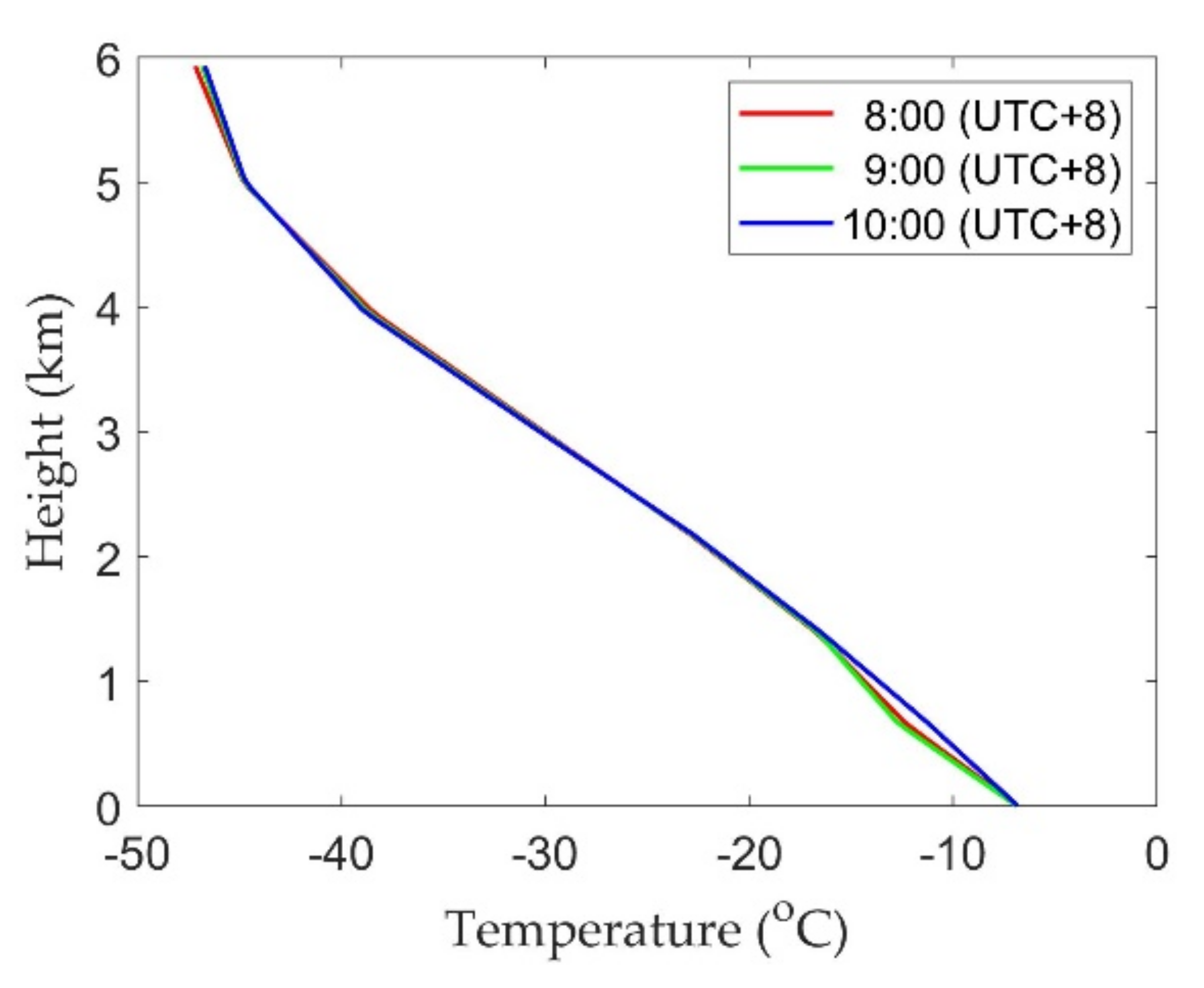
The change in temperature with the time during this event was not significant (see
Figure 5). The temperature gradually decreased with the increase in height, and it decreased to 0 °C at the height of approximately 1.5 km. The “bright band” displayed in
Figure 4 is just near this height level. The “bright band” is the melting layer. The obvious increase in the reflectivity, velocity, and spectrum width in the melting layer is because the ice crystals from the upper layer melt (or partially) into liquid water when falling into the melting layer. Most of them are covered by water. The backscattering cross section of water is larger than that of ice particles, resulting in the increase in radar reflectivity. With the increase in falling speed and particle collisions, the combined effect of cloud droplets and raindrops causes a significant increase in the spectrum width. The melting layer in the
W and
V maps (
Figure 4c–f) is presented throughout the whole process, while it sometimes disappeared on the
Ze map. Although there are no in-situ observational data, it can be inferred from the physical properties measured by the two radars and the temperature profiles that the cloud with height below 1.5 km (temperature greater than 0 °C) is liquid, the 1.5–7 km height is the mixed-phase cloud (the temperature is between 0 °C and −38 °C), and above 7 km (less than −38 °C) is ice-crystal dominated.
Above the melting layer, the highest reflectivity appears in the middle of the cloud (2.5–4 km), reaching approximately 10 dBZ (
Figure 4a). There is some change in the Doppler velocity and spectrum width. From 0900 to 1100, the downward
V and
W increased above the melting layer when compared to other adjacent periods. It might be inferred from this that more hydrometeors from the upper level fell down, resulting in stronger disturbance and larger
W. After that point, the reflectivity increased from 1200 to 1400. It appears that the stronger disturbance helps to break the balance of the cloud system, enhances the possibility of collisions of hydrometeors, and results in large droplets. This precipitation event actually included two precipitation processes with two rainfall peaks, rather than a single process of developing to enhancing and finally decaying. The dual-frequency radar recorded the two precipitation processes, especially the transition process with increasing movement in the upper layer between them.
During the transition process, cloud (rain) droplets entered the area above the melting layer with the airflow, resulting in an evident increase in the spectrum width (see
Figure 4). Theoretically, for a radar bin with uniform particle size distribution, its Doppler spectrum is usually a single-peak distribution, and the spectrum width is relatively low. However, for a radar bin with a diverse and complex particle size distribution, its Doppler spectrum will be a dual or multi-peak distribution, and the Doppler spectrum width will increase. The process from 0900 to 1100 also shows that the spectrum width value is a signal to indicate super-cooled water, which needs further research in the future.
The reflectivity,
V,
W, and LDR differences between the 35- and 94-GHz radar during this event are analyzed (see
Figure 6). There are some dots where the W-band radar has obtained the reflectivity, but the Ka-band radar has not. We use dark blue to mark these dots (the same color has a similar meaning in the following “difference” figures). In the three panels in
Figure 6, dark blue dots mostly appear near the top of the cloud, where the W-band radar reflectivity is lower than that of other interior area. The top of the cloud typically has a lower particle concentration and smaller sizes, resulting in overly weak reflectivity being captured by the Ka-band radar. In this case, the portion of the Ka-band radar that did not obtain the reflectivity was very small and, mostly, both the Ka-band radar and the W-band radar obtained the reflectivity from the cloud. The measurements of the four parameters from the two radars are compared in
Figure 7.
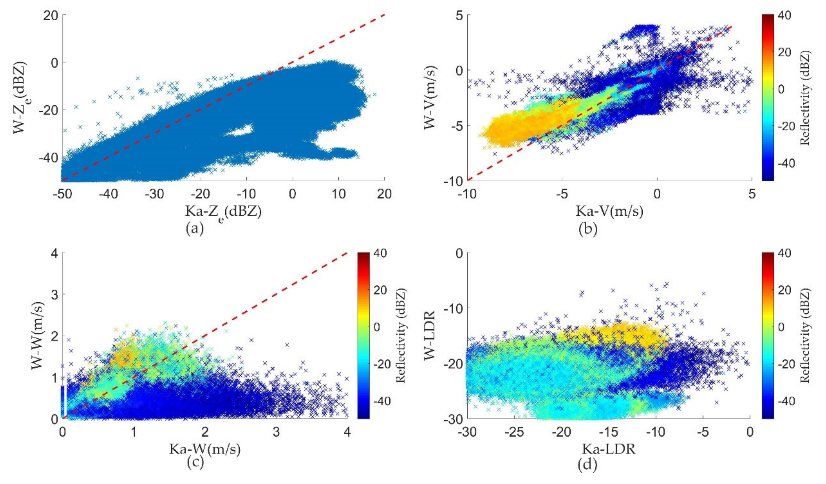
Most of the
Ze values measured by the Ka-band radar are higher than those of the W-band radar (see
Figure 7a). In particular during the time from 0200 to 0300 (see
Figure 6a), all of the reflectivity of the cloud from the Ka-band radar is significantly higher than that of the W-band radar, and the maximum Ka-band radar reflectivity reaches 15 dBZ. High reflectivity below the melting layer is accompanied by severe attenuation due to the liquid droplets, especially for shorter wavelengths. Thus, the
Dze increased significantly during this period (reaching 40 dB). Therefore, high
Dze is normally accompanied by high Ka-band radar reflectivity. It can be inferred that layers where the
Dze is high might be dominated by liquid hydrometeors owing to the larger attenuation for shorter-wavelength radar.
The Ka-band radar is more sensitive to larger cloud particles when compared with the W-band radar. In this case, the difference in
V between the two radars is small when the reflectivity is small (i.e., less than −10 dBZ;
Figure 7b). It can be inferred that the velocity of these particles might be the velocity of the airflow, but not their falling speeds. For particles with large reflectivity (i.e., >0 dBZ, raindrops), the downward
V from the W-band radar is less than the Ka-band radar. The measured
V reflects the falling speed of particles. This case shows that the two radars demonstrate good capability in detecting the velocity. For large reflectivity, the spectrum widths of the Ka-band radar and W-band radar are close. However, for small reflectivity (i.e., less than −40 dBZ), the spectrum widths from the Ka-band radar is more extensive than that from the W-band radar (
Figure 7c). This might be caused by the large uncertainty of the Ka-band radar in detecting the spectrum width for very small particles due to its lower sensitivity. The difference in LDR between two radars is also significant. LDR is the ratio of the power backscattered at vertical polarization (Z
vh) to the power backscattered at horizontal polarization (Z
hh) for the DDCR’s horizontally polarized field, which is strongly dependent on the particle reflectivity and the radar sensitivity. Thus, the uncertainty of LDR is greater than that of radar reflectivity. The complex and chaotic feature in
Figure 7d might be related to the high uncertainty of LDR.
3.2. Cloud Case
The case presented in
Figure 8 occurred between 0000 and 1300 on 3 March 2020. The average CBH was approximately 2 km, and the average cloud depth was approximately 2 km, with a maximum of 3-km depth. The reflectivity measured by the radar in this case is mostly less than −10 dBZ, which is obviously lower than the case in
Section 3.1.
There is no melting layer in
Figure 8. During the time period 0400 to 0600, the cloud thickness and radar reflectivity are relatively larger when compared with other periods. As shown in
Figure 8c, the Ka-band radar also lost some measurements at the edge of the cloud, such as the top of the cloud and the bottom of the cloud, when compared to the W-band radar.
Figure 9 shows the temperature profile from 0800 to 1000 on 3 March 2020. In the height range between 2 km and 4 km, the temperature dropped from approximately −20 °C to approximately −40 °C, and the cloud top temperature was lower than −40 °C. The
Ze,
V,
W and LDR are shown in
Figure 10. In
Figure 10a,c for the Ka-band radar, there are many more pepper-like signals near the cloud-top area. However, the W-band radar does not feature such pepper-like phenomena. The lower signal-to-noise ratio of the Ka-band radar for these signals caused obvious uncertainties in detecting the
V and
W. Moreover, due to the very weak signal, the Ka-band radar obtained the LDR values of a very small portion of the whole cloud. In this case, the W-band radar performs better than the Ka-band radar.
According to the temperature profile and the distribution characteristics of the radar reflectivity, for example, there is no melting layer, and
Dze changes little with height (see
Figure 8c), from which it can be concluded that ice crystals dominated in the cloud and the droplet size was small. In order to further understand the performance of the DDCR, we also compared the four parameters (
Ze,
V,
W, and LDR) measured by the two radars for this case (see
Figure 11). For the measurements both radars obtained, the reflectivity measured by the W-band radar is generally higher than the Ka-band radar, and most
Ze values are less than −10 dBZ. The statistical results show that the average value of
Dze in this case is −2.9 dBZ, and the minimum
Dze reaches −15 dBZ. The velocities measured by the two radars are close. Most of the spectrum width is less than 0.4 m/s, indicating a uniform particle distribution function.
In terms of Rayleigh scattering, the backscattering cross section σ of a small spherical particle can be expressed as:
According to the radar Equation (1), the effective reflectivity factor Z
e will be:
As seen from Equation (7), the
Ze only depends on the cloud particle size distribution, and ideally should not be linked with the wavelength. In this case, and the case in
Section 3.1, the reflectivity measured by the Ka-band radar and W-band radar demonstrates an obvious discrepancy. The attenuation by cloud and gas is one cause, since it has different impacts for different wavelengths. In addition, the Rayleigh scattering assumption for Equation (6) might be inapplicable at times for the two wavelengths. Here, in this case, the average reflectivity is relatively low and the reflectivity measured by the W-band radar is mostly higher than that of the Ka-band radar. Besides the causes generated by the Rayleigh scattering assumption, there are four other possible reasons:
- (1)
As presented in the radar Equation (1), the different uncertainty of the radar constant between the Ka-band radar and W-band radar will cause a difference in Ze;
- (2)
The value of K in Equation (3) is fixed. The K value of liquid particles increases with the increase in wavelength, while the K value of ice particles is small and changes less with wavelength. When an actual cloud particle is ice rather than liquid, the K should be adjusted according to the wavelength and particle phase. When such an adjustment is absent, the Ze value measured by the W-band radar is destined to be higher than the Ze measured by the Ka-band radar;
- (3)
The Ze obtained by the radar is the echo from a scatter volume. The larger particles in the volume contribute much more reflectivity than small particles. The Ka-band radar and W-band radar have different sensitivities to different sizes of particles, resulting in different Ze when the integral scattering of large particles and small particles is different;
- (4)
The Ka-band radar has a wider beam-width than the W-band radar. In fact, the volume they detected was not quite the same.
The difference caused by reason (1) can be minimized by the calibration experiment. The differences caused by the other three reasons are linked with the physical properties of the particles themselves. Thus, the difference of reflectivity, velocity, etc., between the Ka-band and W-band radar data imply the microphysical properties of cloud (i.e., size, phase), and presents ultra-information that can be used to retrieve microphysical characteristics of the particles in the cloud.
3.3. Ice Cloud Case
Ice crystals account for the absolute majority of ice clouds. The previous studies of Ka-band or W-band attenuation in ice clouds and water clouds indicate that the attenuation by ice is far smaller than by liquid hydrometeors must be considered [
10,
29,
30].
Figure 12 shows the measurements of DDCR on 19 February 2020. The temperature profile of the day (1400–2200, with an interval of 2 h) is shown in
Figure 13. The temperature at 1400 at the height of 4 km reached −38 °C. From 1400 to 1700, the CBH detected by the W-band radar was approximately 4 km. It can be concluded that it was ice cloud during this period.
The observations of the W-band radar (see
Figure 12b) show that there were continuous clouds between the heights of 3 km and 7 km from 1400 to 2400. However, the Ka-band radar (see
Figure 12a) did not obtain the cloud returning until 1800. Moreover, the cloud it measured was a portion of the cloud measured by the W-band radar, and the upper-layer cloud was missed by the Ka-band radar. The CTH measured by the Ka-band radar was almost 1 km lower than that of the W-band radar. According to the temperature profile and the radar reflectivity value, mixed-phase cloud began to appear after 1800, the cloud thickened, and some of the backscattering cross section increased. When cloud particles are ice crystals, the particle sizes and number concentration are small, and their backscattering cross-section is small. When the reflectivity is lower than the radar sensitivity, these particles will be lost by the radar. In this case, the Ka-band radar did not detect the cloud from 1400 to 1700, as well as some upper-layer cloud owing to their weak return.
All of the reflectivity that both the Ka-band radar and W-band radar obtained is presented and compared in
Figure 14a. The maximum
Ze in this case was approximately −10 dBZ. Most of the reflectivity measured by the Ka-band radar was lower than that of the W-band radar. The average
Dze was −5.1 dBZ.
Figure 14b shows a histogram of the W-band radar
Ze for the cloud that the Ka-band radar did not detect. As seen from
Figure 14b, the W-band radar
Ze was generally lower than −20 dBZ and the average reflectivity was −33.5 dBZ. We divided the cloud above 3 km into two categories: the cloud only the W-band radar detected, and the cloud that both the W-band and Ka-band radar detected.
Figure 14c shows the W-band radar reflectivity and the height for the two cloud categories. Through comparison, it can be seen that the Ka-band radar lost some cloud, mainly due to its low sensitivity. Interestingly, the reflectivity of the two categories is not completely separated, but partly overlapped (i.e., between −30 dBZ and −25 dBZ); that is, the Ka-band radar can sometimes receive echoes, but sometimes cannot when the W-band radar reflectivity is between −30 dBZ and −25 dBZ. The possible reason for this might be the difference in the filling coefficient and the particle distribution function. However, more observations by other instruments are needed to gain a deeper understanding.
3.4. Cloud-Top Height and Cloud-Base Height
We selected one year of non-precipitating cloud data from August 2019 to August 2020 and compared the CTH and CBH observed by the W-band radar and Ka-band radar. For each cloud profile, the highest height and lowest height were recorded. The median CTH and CBH of all profiles within 10 min were then calculated.
Figure 15 shows the CTH and CBH of a cloud case calculated every ten minutes on 15 December 2019.
Figure 16a shows the CBHs measured by the Ka-band and W-band radars when both radars observed the CBH. The year’s data were divided into two parts: the warm season (orange, May to October), and the cold season (blue). It can be seen that the CBHs from the Ka-band radar and W-band radar are mostly concentrated around the 1:1 line. The distribution in the cold season is relatively tighter than in the warm season. There are several cases in the warm season, in which the CBH measured by the W-band radar is far from that of the Ka-band radar. The statistical results (see
Figure 16c) show that the average difference in CBH (D
CBH) between the two radars is very small, at approximately 0.06 km.
Figure 16b shows the contrast in the CTH. In both the warm and cold seasons, it can be seen that more points are located above the 1:1 line, indicating that most of the CTHs measured by the W-band radar are higher than the values measured by the Ka-band radar. The average difference is −0.6 km (see
Figure 16d), which means that the CTH measured by the W-band radar is on average 600 m higher than that measured by the Ka-band radar. It should be noted that the statistical results here are based on all non-precipitating clouds, since there is large uncertainty in the CBH of precipitation. The concentration and size of cloud particles near the top is generally relatively low and small compared with the middle cloud, and the temperature at Yangbajing is relatively low, especially in the cold season. Therefore, the upper cloud is more likely to be dominated by ice crystals. These factors challenge the detection capability of the Ka-band radar, which has lower sensitivity. The case analyses show that, in general, the W-band radar performs better than the Ka-band radar in the detection of non-precipitating clouds at the Yangbajing study site.
4. Discussion
Radar transmits the wave with beam-width, and the reflectivity radar measures is the integral of all cloud particles in a volume. The Ka-band radar uses a wavelength of 8 mm, which is almost 2–3 times that of the W-band radar (3 mm); thus, essentially, they should have different sensitivities to different cloud particles. Therefore, even if the calibration, data quality control, attenuation correction, etc., are perfectly solved, the measurements for the same volume made by the Ka-band radar and W-band radar should perform differently, since the volume contains particles with various physical characteristics (such as size, phase, shape, etc.). The advantages and disadvantages of the DDCR have been revealed in this paper, not from theory, but through investigation different clouds observed in a field campaign. The comparisons made in this paper are preliminary; however, the results provide a reference for subsequent data processing and applications of the two radars. For example, the differences in reflectivity between the two radars demonstrate the particle phase and size properties, which helps to improve the inversion accuracy of microphysical characteristics of cloud and precipitation. Therefore, simultaneous and synergetic measurements of dual-frequency radars provide more information on cloud and precipitation. In the future, it is hoped that some new knowledge regarding clouds and precipitation can be obtained or revealed through further research and analysis.
We can “see” other parts of the cloud that the Ka-band radar fails to capture by the W-band radar. But does this mean that the current W-band radar has been able to detect the entire cloud? If not, what percentage does it miss? The technique of radar has always been, and continues to be, complex and challenging. However, radar is a powerful instrument to explore the interior of clouds and their changes, thus providing an opportunity for a comprehensive understanding of clouds—one of the most important aspects of nature. It is therefore certainly worth carrying out more research of this type in the future.


