
Characterization of Dry-Season Phenology in Tropical Forests by Reconstructing Cloud-Free Landsat Time Series

 ,
,  , ,
, ,
Abstract
:1. Introduction
2. Study Area and Data Used
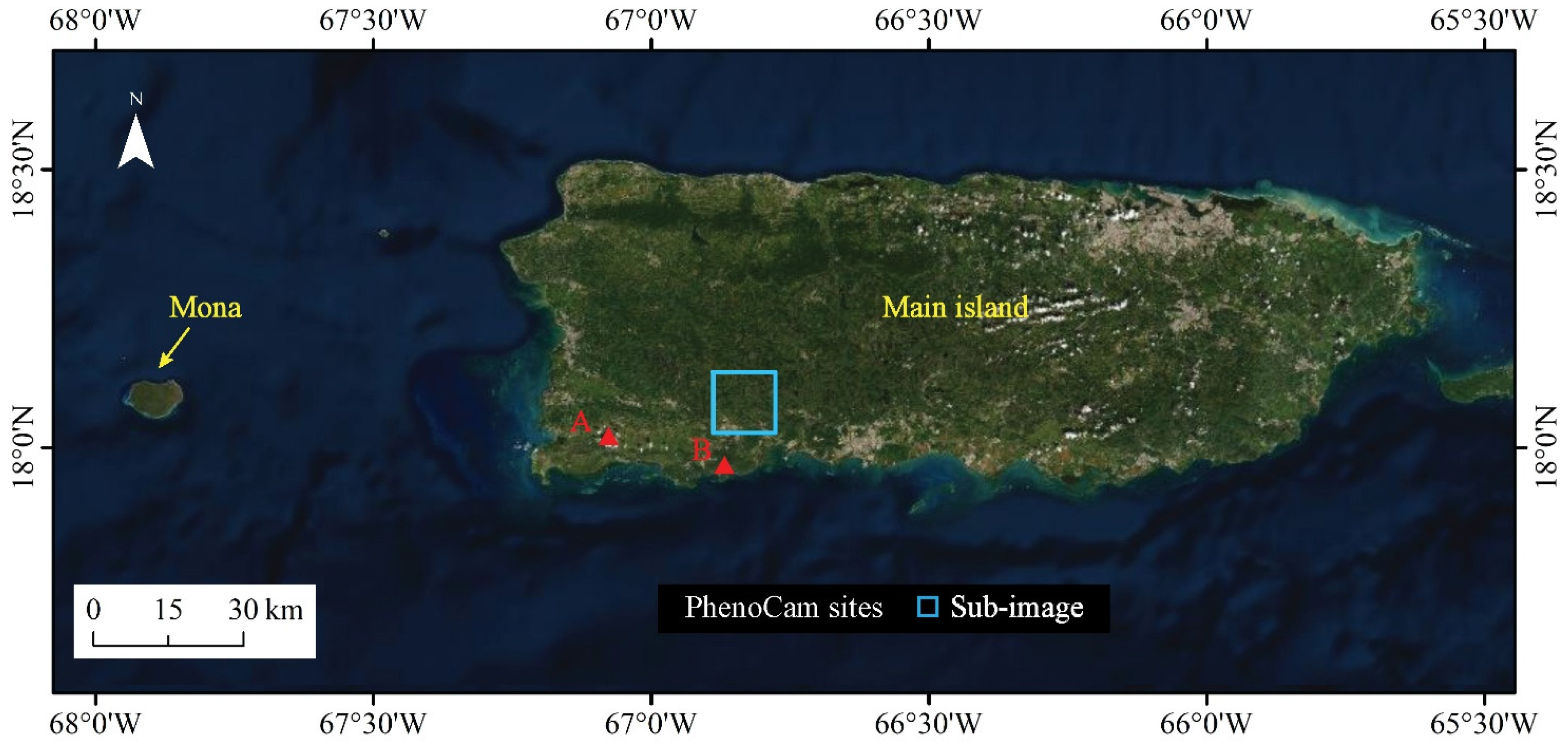
2.1. Study Area
2.2. Data Used
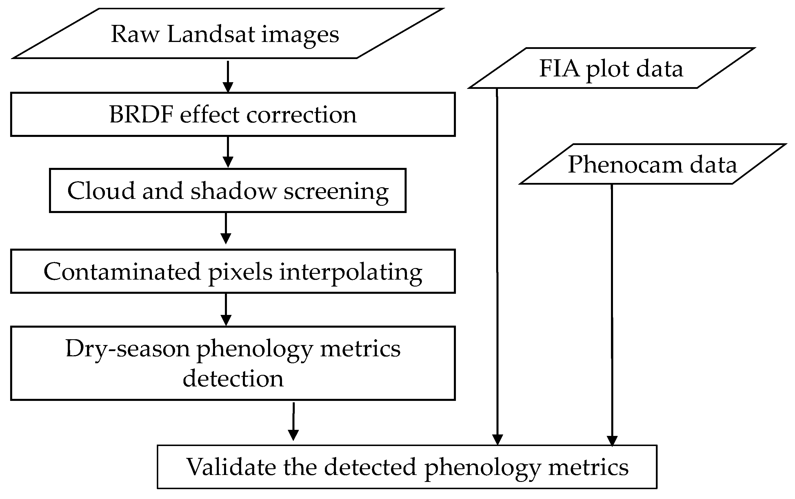
3. Methods
3.1. Generating a Cloud-Free Seasonal Landsat Time Series
3.1.1. BRDF Effect Correction
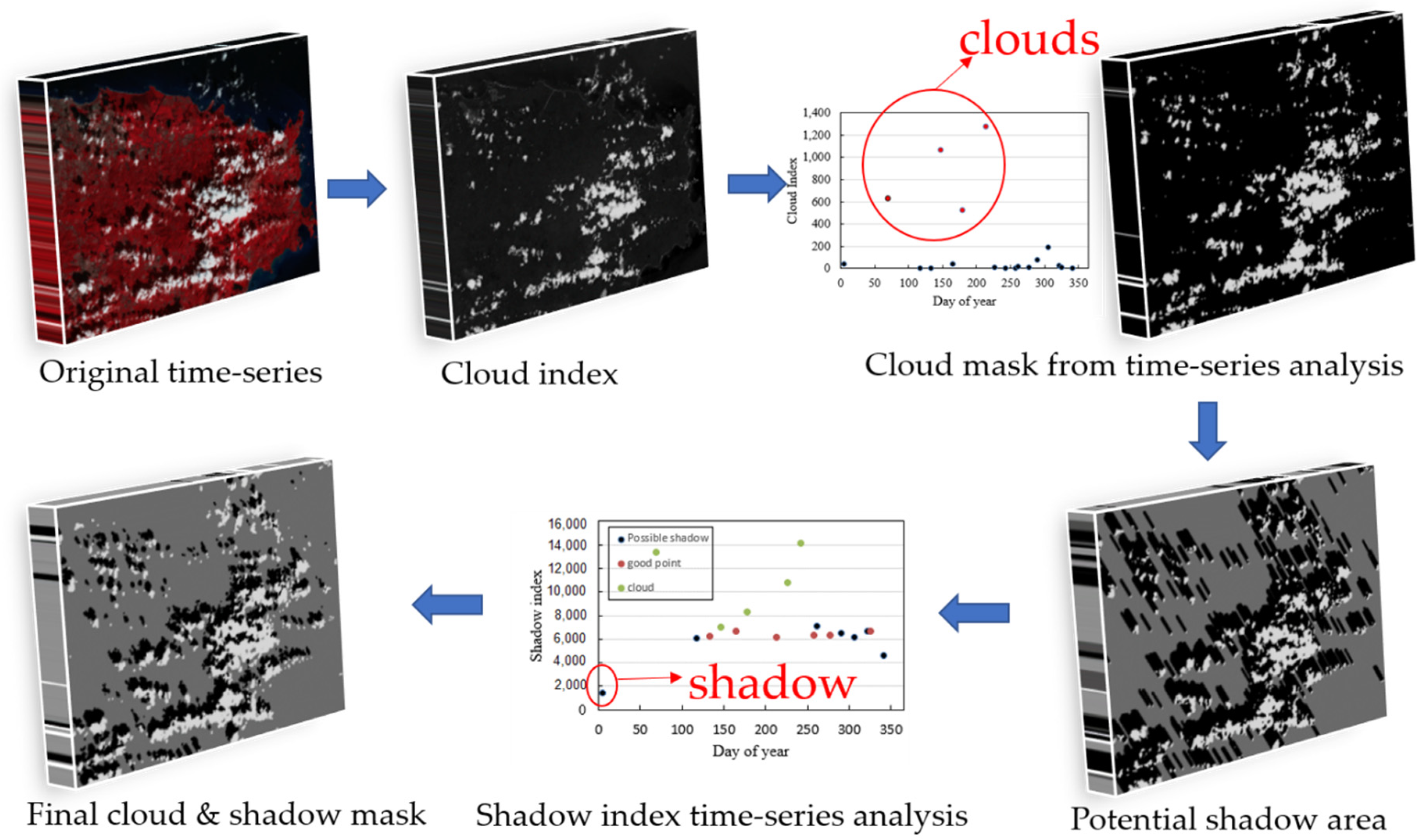
3.1.2. Screening Clouds and Cloud Shadows
3.1.3. Interpolating Contaminated Pixels in the Time Series
3.2. Extracting the Phenological Metrics
3.3. Validation
4. Results
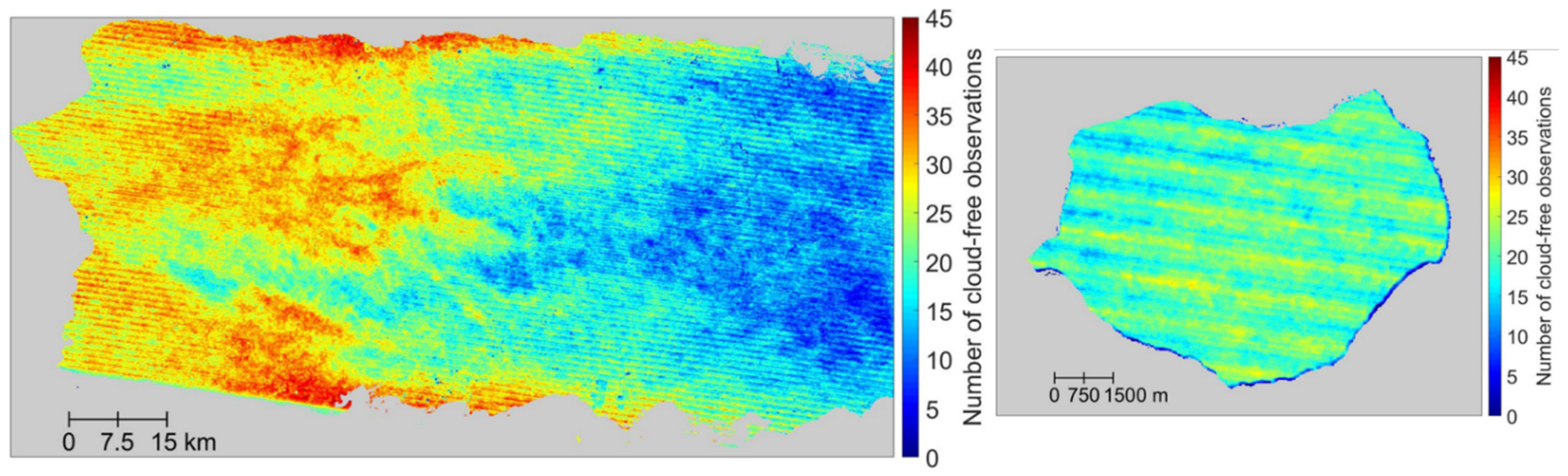
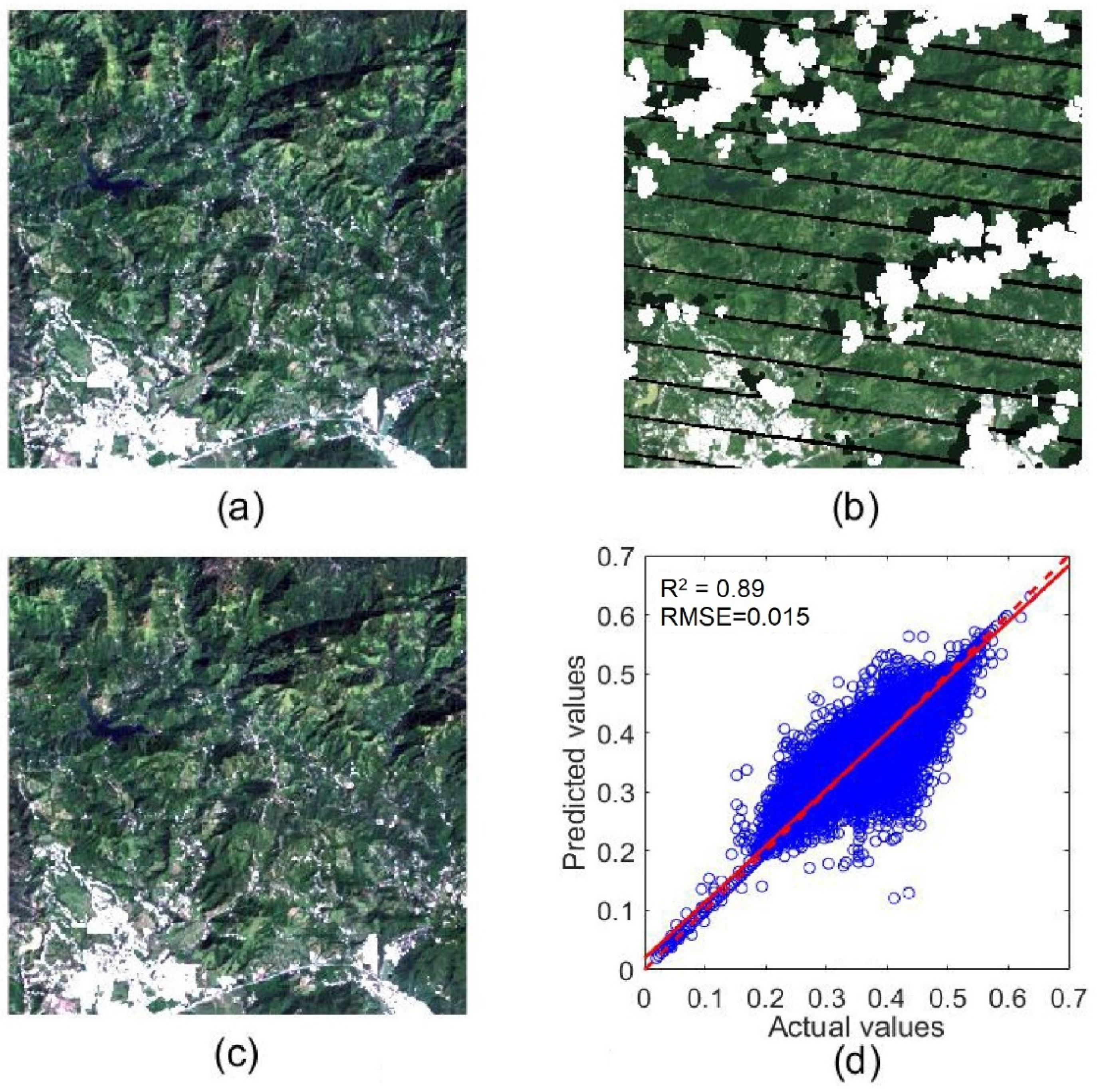
4.1. Accuracy of Landsat Time Series Reconstruction
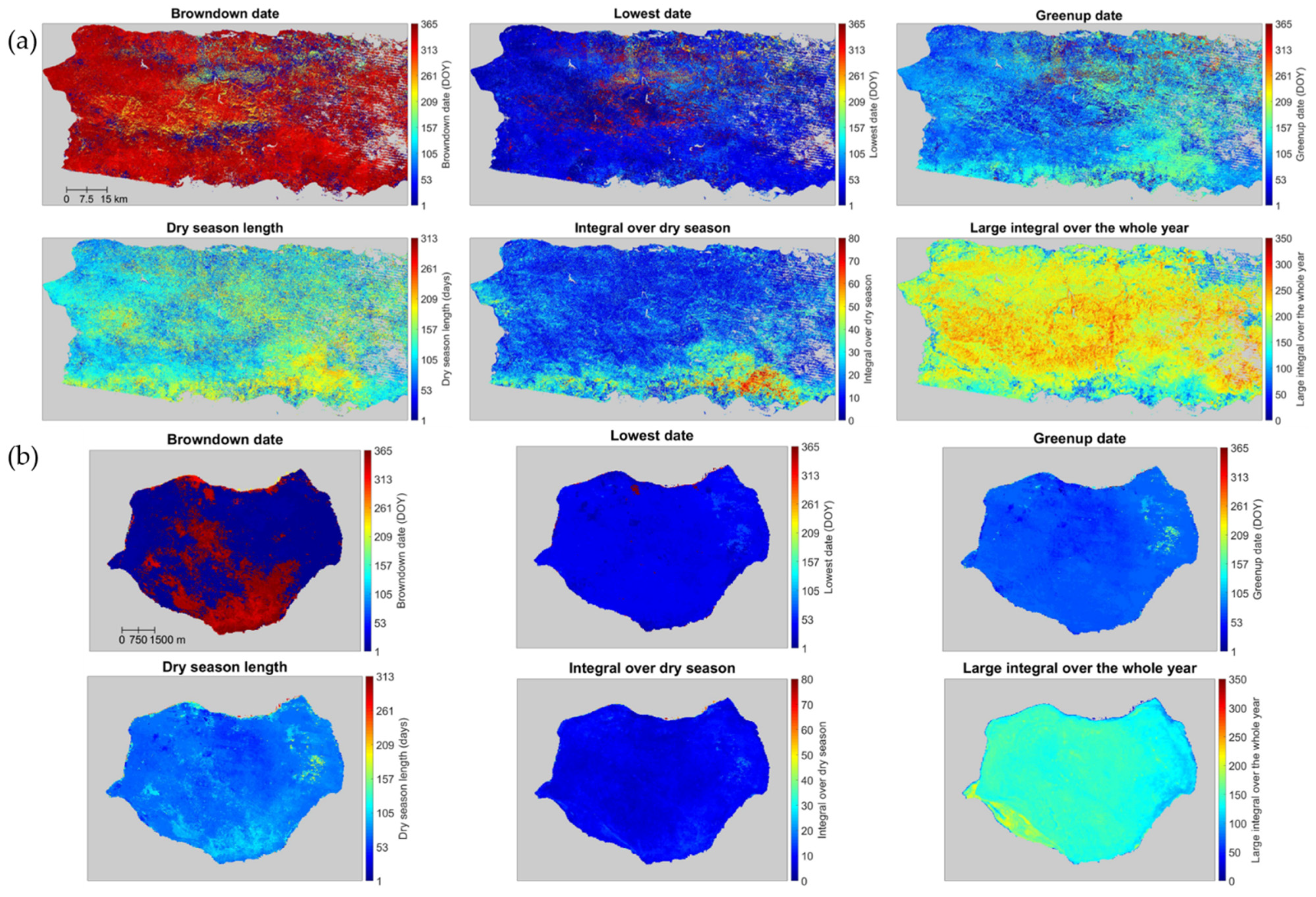
4.2. Maps and Reasonability of Detected Phenology Metrics
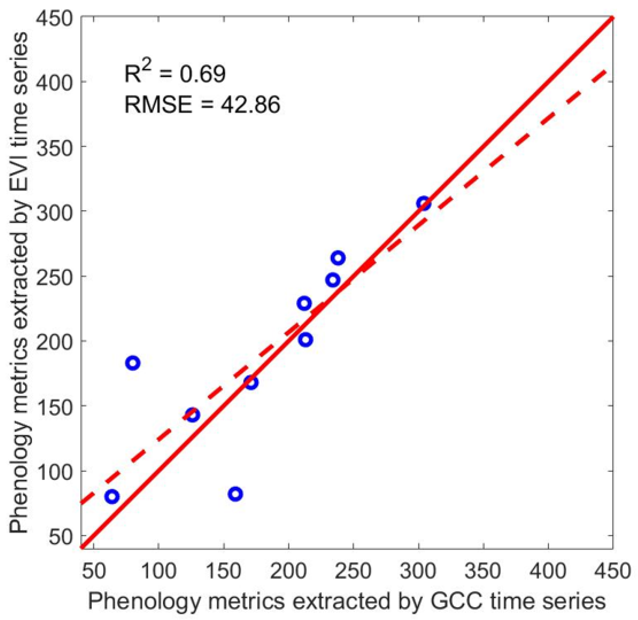
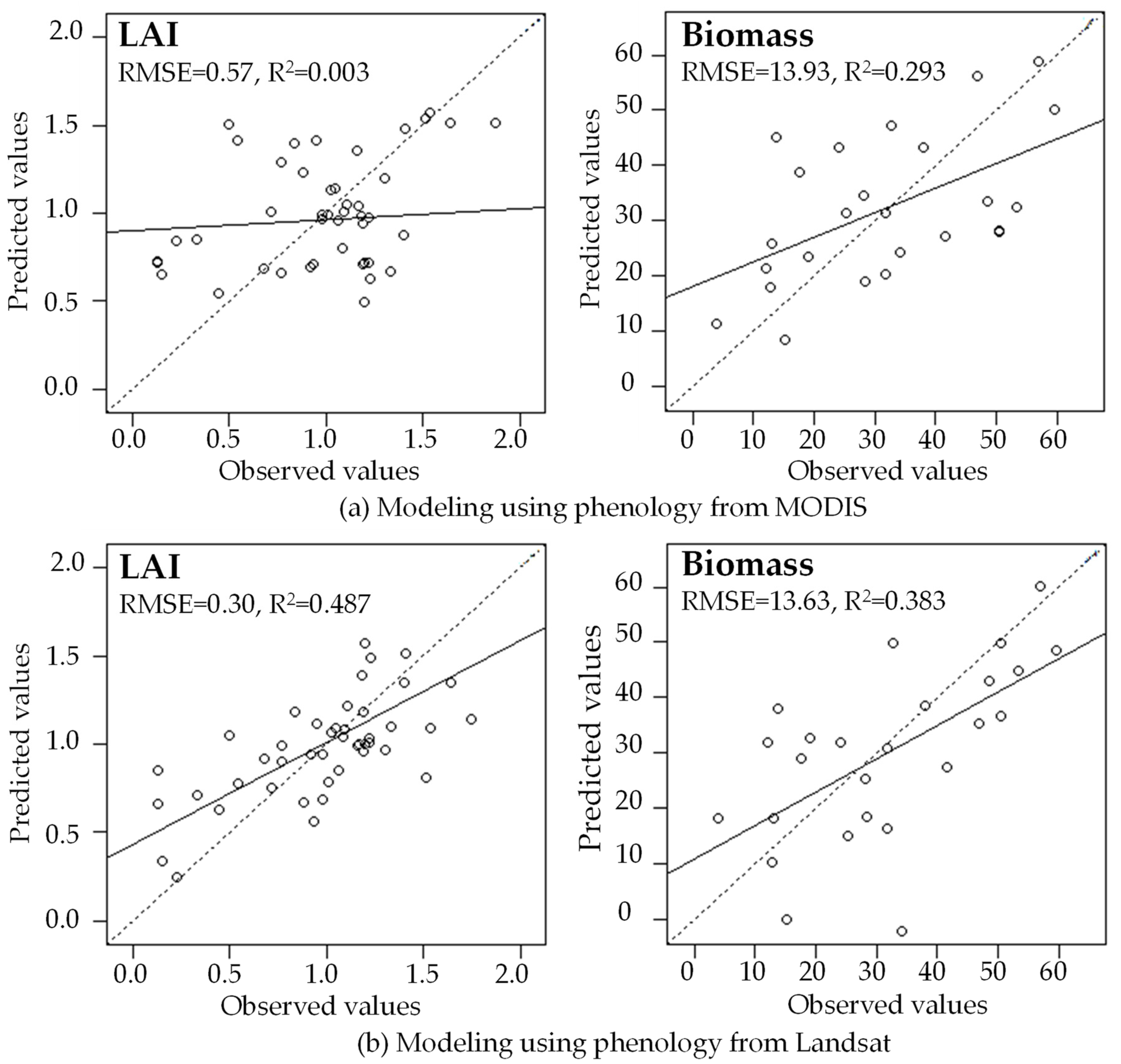
4.3. Validation Results of Detected Phenology Metrics
5. Discussion
5.1. Implications for Tropical Forest Monitoring
5.2. Limitations and Future Studies
6. Conclusions
Author Contributions
Funding
Institutional Review Board Statement
Informed Consent Statement
Data Availability Statement
Conflicts of Interest
References
- Bustamante, M.; Helmer, E.H.; Schill, S.; Belnap, J.; Brown, L.K.; Brugnoli, E.; Compton, J.E.; Coupe, R.H.; Hernández-Blanco, M.; Isbell, F.; et al. Chapter 4: Direct and indirect drivers of change in biodiversity and nature’s contributions to people. In Regional Assessment Report on Biodiversity and Ecosystem Services for the Americas; IPBES Secretariat: Bonn, Germany, 2018; pp. 335–509. [Google Scholar]
- Jiang, Y.; Zhou, L.; Tucker, C.J.; Raghavendra, A.; Hua, W.; Liu, Y.Y.; Joiner, J. Widespread increase of boreal summer dry season length over the Congo rainforest. Nat. Clim. Chang. 2019, 9, 617–622. [Google Scholar] [CrossRef]
- Sarvia, F.; De Petris, S.; Borgogno-Mondino, E. Exploring Climate Change Effects on Vegetation Phenology by MOD13Q1 Data: The Piemonte Region Case Study in the Period 2001–2019. Agronomy 2021, 11, 555. [Google Scholar] [CrossRef]
- Asner, G.P.; Alencar, A. Drought impacts on the Amazon forest: The remote sensing perspective. New Phytol. 2010, 187, 569–578. [Google Scholar] [CrossRef] [PubMed]
- Brando, P.M.; Balch, J.K.; Nepstad, D.C.; Morton, D.C.; Putz, F.E.; Coe, M.T.; Silvério, D.; Macedo, M.N.; Davidson, E.A.; Nóbrega, C.C.; et al. Abrupt increases in Amazonian tree mortality due to drought—Fire interactions. Proc. Natl. Acad. Sci. USA 2014, 111, 6347–6352. [Google Scholar] [CrossRef] [Green Version]
- Briant, G.; Gond, V.; Laurance, S.G.W. Habitat fragmentation and the desiccation of forest canopies: A case study from eastern Amazonia. Biol. Conserv. 2010, 143, 2763–2769. [Google Scholar] [CrossRef]
- Baker, J.C.A.; Spracklen, D.V. Climate Benefits of Intact Amazon Forests and the Biophysical Consequences of Disturbance. Front. For. Glob. Chang. 2019, 2, 47. [Google Scholar] [CrossRef] [Green Version]
- Allen, C.D.; Macalady, A.K.; Chenchouni, H.; Bachelet, D.; Mcdowell, N.; Vennetier, M.; Kitzberger, T.; Rigling, A.; Breshears, D.D.; Hogg, E.H.T.; et al. A global overview of drought and heat-induced tree mortality reveals emerging climate change risks for forests. For. Ecol. Manag. 2010, 259, 660–684. [Google Scholar] [CrossRef] [Green Version]
- Zhang, Q.; Shao, M.; Jia, X.; Wei, X. Relationship of Climatic and Forest Factors to Drought- and Heat-Induced Tree Mortality. PLoS ONE 2017, 12, e0169770. [Google Scholar] [CrossRef]
- Mcdowell, N.; Mcdowell, N.; Allen, C.D.; Anderson-teixeira, K.; Brando, P.; Brienen, R.; Chambers, J.; Christoffersen, B.; Davies, S.; Doughty, C.; et al. Drivers and mechanisms of tree mortality in moist tropical forests. New Phytol. 2018, 219, 851–869. [Google Scholar] [CrossRef] [Green Version]
- Powers, J.S.; Vargas, G.; Brodribb, G.T.J.; Schwartz, N.B.; Chris, D.P.; Becknell, J.M.; Aureli, F.; Calderón-morales, R.B.E.; Ana, J.C.C.; María, J.C.; et al. A catastrophic tropical drought kills hydraulically vulnerable tree species. Glob. Chang. Biol. 2020, 26, 3122–3133. [Google Scholar] [CrossRef]
- Mitchard, E.T.A. The tropical forest carbon cycle and climate change. Nature 2018, 559, 2–9. [Google Scholar] [CrossRef]
- Gardner, T.A.; Barlow, J.; Chazdon, R.; Robert, M.; Harvey, C.A. Prospects for tropical forest biodiversity in a human-modified world. Ecol. Lett. 2009, 12, 561–582. [Google Scholar] [CrossRef] [Green Version]
- Barlow, J.; França, F.; Gardner, T.A.; Hicks, C.C.; Lennox, G.D.; Berenguer, E.; Castello, L.; Economo, P.; Ferreira, J.; Guénard, B.; et al. The future of hyperdiverse tropical ecosystems. Nature 2018, 559, 517–526. [Google Scholar] [CrossRef]
- Bi, J.; Knyazikhin, Y.; Choi, S.; Park, T.; Jonathan, B.; Philippe, C.; Fu, R.; Ganguly, S.; Hall, F.; Hilker, T.; et al. Sunlight mediated seasonality in canopy structure and photosynthetic activity of Amazonian rainforests. Environ. Res. Lett. 2015, 10, 64014. [Google Scholar] [CrossRef] [Green Version]
- Cooley, S.S.; Williams, C.A.; Fisher, J.B.; Halverson, G.H.; Perret, J.; Lee, C.M. Assessing regional drought impacts on vegetation and evapotranspiration: A case study in Guanacaste, Costa Rica. Ecol. Appl. 2019, 29, e01834. [Google Scholar] [CrossRef]
- Gonçalves, N.B.; Lopes, A.P.; Dalagnol, R.; Wu, J.; Pinho, D.M.; Nelson, B.W. Both near-surface and satellite remote sensing confirm drought legacy effect on tropical forest leaf phenology after 2015/2016 ENSO drought. Remote Sens. Environ. 2020, 237, 111489. [Google Scholar] [CrossRef]
- Wang, J.; Yang, D.; Detto, M.; Nelson, B.W.; Chen, M.; Guan, K.; Wu, S.; Yan, Z.; Wu, J. Multi-scale integration of satellite remote sensing improves characterization of dry-season green-up in an Amazon tropical evergreen forest. Remote Sens. Environ. 2020, 246, 111865. [Google Scholar] [CrossRef]
- Helmer, E.H.; Ruzycki, T.S.; Wilson, B.T.; Sherrill, K.R.; Lefsky, M.A.; Marcano-Vega, H.; Brandeis, T.J.; Erickson, H.E.; Ruefenacht, B. Tropical Deforestation and Recolonization by Exotic and Native Trees: Spatial Patterns of Tropical Forest Biomass, Functional Groups, and Species Counts and Links to Stand Age, Geoclimate, and Sustainability Goals. Remote Sens. 2018, 10, 1724. [Google Scholar] [CrossRef] [Green Version]
- Roa-Fuentes, L.L.; Templer, P.H.; Campo, J. Effects of precipitation regime and soil nitrogen on leaf traits in seasonally dry tropical forests of the Yucatan Peninsula, Mexico. Oecologia 2015, 179, 585–597. [Google Scholar] [CrossRef] [PubMed]
- Umaña, M.N.; Wright, S.J.; Condit, R.; Pérez, R.; Turner, B.L.; Comita, L.S. Shifts in taxonomic and functional composition of trees along rainfall and phosphorus gradients in central Panama. J. Ecol. 2020, 109, 51–61. [Google Scholar] [CrossRef]
- Ruger, N.; Comita, L.S.; Condit, R.; Purves, D.; Rosenbaum, B.; Visser, M.D.; Wright, S.J.; Wirth, C. Beyond the fast—Slow continuum: Demographic dimensions structuring a tropical tree community. Ecol. Lett. 2018, 21, 1075–1084. [Google Scholar] [CrossRef] [Green Version]
- Rozendaal, D.M.A.; Phillips, O.L.; Lewis, S.L.; Affum-baffoe, K.; Alvarez-davila, E.; Andrade, A.; Banki, O.; Aragao, L.E.O.C.; Baker, T.R.; Brienen, R.J.W.; et al. Competition influences tree growth, but not mortality, across environmental gradients in Amazonia and tropical Africa. Ecology 2020, 101, e03052. [Google Scholar] [CrossRef]
- Wieczynski, D.J.; Singla, P.; Doan, A.; Singleton, A.; Han, Z.; Votzke, S.; Yammine, A.; Gibert, J.P. Simple traits predict complex temperature responses across ecological scales. Res. Sq. 2021. [Google Scholar] [CrossRef]
- Newman, E.A.; Breckheimer, I.K.; Park, D.S. Disentangling the effects of climate change, landscape heterogeneity, and scale on phenological metrics. bioRxiv 2021, 1–20. [Google Scholar] [CrossRef]
- Tian, J.; Zhu, X.; Wu, J.; Shen, M.; Chen, J. Coarse-Resolution Satellite Images Overestimate Urbanization Effects on Vegetation Spring Phenology. Remote Sens. 2020, 12, 117. [Google Scholar] [CrossRef] [Green Version]
- Melaas, E.K.; Friedl, M.A.; Zhu, Z. Detecting interannual variation in deciduous broadleaf forest phenology using Landsat TM/ETM+ data. Remote Sens. Environ. 2013, 132, 176–185. [Google Scholar] [CrossRef]
- Kowalski, K.; Senf, C.; Hostert, P.; Pflugmacher, D. Characterizing spring phenology of temperate broadleaf forests using Landsat and Sentinel-2 time series. Int. J. Appl. Earth Obs. Geoinf. 2020, 92, 102172. [Google Scholar] [CrossRef]
- Jönsson, P.; Cai, Z.; Melaas, E.; Friedl, M.A.; Eklundh, L. A method for robust estimation of vegetation seasonality from Landsat and Sentinel-2 time series data. Remote Sens. 2018, 10, 635. [Google Scholar] [CrossRef] [Green Version]
- Modica, G.; Solano, F.; Merlino, A.; Di Fazio, S.; Barreca, F.; Laudari, L.; Fichera, C.R. Using Landsat 8 imagery in detecting cork oak (Quercus suber L.) woodlands: A case study in Calabria (Italy). J. Agric. Eng. 2016, 47, 205–215. [Google Scholar] [CrossRef] [Green Version]
- Zhang, M.; Gong, P.; Qi, S.; Liu, C.; Xiong, T. Mapping bamboo with regional phenological characteristics derived from dense Landsat time series using Google Earth Engine. Int. J. Remote Sens. 2019, 40, 9541–9555. [Google Scholar] [CrossRef]
- Praticò, S.; Solano, F.; Di Fazio, S.; Modica, G. Machine Learning Classification of Mediterranean Forest Habitats in Google Earth Engine Based on Seasonal Sentinel-2 Time-Series and Input Image Composition Optimisation. Remote Sens. 2021, 13, 586. [Google Scholar] [CrossRef]
- King, L.; Adusei, B.; Stehman, S.V.; Potapov, P.V.; Song, X.; Krylov, A.; Di, C.; Loveland, T.R.; Johnson, D.M.; Hansen, M.C. A multi-resolution approach to national-scale cultivated area estimation of soybean. Remote Sens. Environ. 2017, 195, 13–29. [Google Scholar] [CrossRef]
- Song, X.; Potapov, P.V.; Krylov, A.; King, L.; Di, C.M.; Hudson, A.; Khan, A.; Adusei, B.; Stehman, S.V.; Hansen, M.C. National-scale soybean mapping and area estimation in the United States using medium resolution satellite imagery and field survey. Remote Sens. Environ. 2017, 190, 383–395. [Google Scholar] [CrossRef]
- Bendini, H.N.; Fonseca, L.M.G.; Schwieder, M.; Körting, T.S.; Rufin, P.; Sanches, I.D.A.; Leitão, P.J.; Hostert, P. Detailed agricultural land classification in the Brazilian cerrado based on phenological information from dense satellite image time series. Int. J. Appl. Earth Obs. Geoinf. 2019, 82, 101872. [Google Scholar] [CrossRef]
- Zhu, X.; Helmer, E.H. An automatic method for screening clouds and cloud shadows in optical satellite image time series in cloudy regions. Remote Sens. Environ. 2018, 214, 135–153. [Google Scholar] [CrossRef]
- Zhu, Z.; Woodcock, C.E. Object-based cloud and cloud shadow detection in Landsat imagery. Remote Sens. Environ. 2012, 118, 83–94. [Google Scholar] [CrossRef]
- Foga, S.; Scaramuzza, P.L.; Guo, S.; Zhu, Z.; Dilley, R.D.; Beckmann, T.; Schmidt, G.L.; Dwyer, J.L.; Joseph Hughes, M.; Laue, B. Cloud detection algorithm comparison and validation for operational Landsat data products. Remote Sens. Environ. 2017, 194, 379–390. [Google Scholar] [CrossRef] [Green Version]
- Zhu, X.; Helmer, E.H.; Chen, J.; Liu, D. An Automatic System for Reconstructing High-Quality Seasonal Landsat Time Series. In Remote Sensing Time Series Image Processing; Weng, Q., Ed.; CRC Press: Boca Raton, FL, USA, 2018; pp. 47–64. [Google Scholar]
- Li, X.; Shen, H.; Zhang, L.; Zhang, H.; Yuan, Q.; Yang, G. Recovering Quantitative Remote Sensing Products Contaminated by Thick Clouds and Shadows Using Multitemporal Dictionary Learning. IEEE Trans. Geosci. Remote Sens. 2014, 52, 7086–7098. [Google Scholar] [CrossRef]
- Roy, D.P.; Zhang, H.K.; Ju, J.; Gomez-Dans, J.L.; Lewis, P.E.; Schaaf, C.B.; Sun, Q.; Li, J.; Huang, H.; Kovalskyy, V. A general method to normalize Landsat reflectance data to nadir BRDF adjusted reflectance. Remote Sens. Environ. 2016, 176, 255–271. [Google Scholar] [CrossRef] [Green Version]
- Morton, D.C.; Nagol, J.; Carabajal, C.C.; Rosette, J.; Palace, M.; Cook, B.D.; Vermote, E.F.; Harding, D.J.; North, P.R.J. Amazon forests maintain consistent canopy structure and greenness during the dry season. Nature 2014, 506, 221–224. [Google Scholar] [CrossRef]
- Petri, C.A.; Galvão, L.S. Sensitivity of Seven MODIS Vegetation Indices to BRDF Effects during the Amazonian Dry Season. Remote Sens. 2019, 11, 1650. [Google Scholar] [CrossRef] [Green Version]
- Nagol, J.R.; Sexton, J.O.; Kim, D.-H.; Anand, A.; Morton, D.; Vermote, E.; Townshend, J.R. Bidirectional effects in Landsat reflectance estimates: Is there a problem to solve? ISPRS J. Photogramm. Remote Sens. 2015, 103, 129–135. [Google Scholar] [CrossRef]
- Ross, J. The Radiation Regime and Architecture of Plant Stands; Springer: Dordrecht, The Netherlands, 1981. [Google Scholar] [CrossRef]
- Li, X.; Strahler, A.H. Geometric-Optical Bidirectional Reflectance Modeling of the Discrete Crown Vegetation Canopy: Effect of Crown Shape and Mutual Shadowing. IEEE Trans. Geosci. Remote Sens. 1992, 30, 276–292. [Google Scholar] [CrossRef]
- Ju, J.; Roy, D.P. The availability of cloud-free Landsat ETM+ data over the conterminous United States and globally. Remote Sens. Environ. 2008, 112, 1196–1211. [Google Scholar] [CrossRef]
- Zeng, L.; Wardlow, B.D.; Xiang, D.; Hu, S.; Li, D. A review of vegetation phenological metrics extraction using time-series, multispectral satellite data. Remote Sens. Environ. 2020, 237, 111511. [Google Scholar] [CrossRef]
- Zhang, Q.; Yuan, Q.; Li, J.; Li, Z.; Shen, H.; Zhang, L. Thick cloud and cloud shadow removal in multitemporal imagery using progressively spatio-temporal patch group deep learning. ISPRS J. Photogramm. Remote Sens. 2020, 162, 148–160. [Google Scholar] [CrossRef]
- Yin, G.; Mariethoz, G.; Sun, Y.; McCabe, M.F. A comparison of gap-filling approaches for Landsat-7 satellite data. Int. J. Remote Sens. 2017, 38, 6653–6679. [Google Scholar] [CrossRef]
- Chen, J.; Zhu, X.; Vogelmann, J.E.; Gao, F.; Jin, S. A simple and effective method for filling gaps in Landsat ETM+ SLC-off images. Remote Sens. Environ. 2011, 115, 1053–1064. [Google Scholar] [CrossRef]
- Zhu, X.; Gao, F.; Liu, D.; Chen, J. A modified neighborhood similar pixel interpolator approach for removing thick clouds in landsat images. IEEE Geosci. Remote Sens. Lett. 2012, 9, 521–525. [Google Scholar] [CrossRef]
- Zhang, X.; Friedl, M.A.; Schaaf, C.B.; Strahler, A.H.; Hodges, J.C.; Gao, F.; Reed, B.C.; Huete, A. Monitoring vegetation phenology using MODIS. Remote Sens. Environ. 2003, 84, 471–475. [Google Scholar] [CrossRef]
- Shang, R.; Liu, R.; Xu, M.; Liu, Y.; Zuo, L.; Ge, Q. The relationship between threshold-based and inflexion-based approaches for extraction of land surface phenology. Remote Sens. Environ. 2017, 199, 167–170. [Google Scholar] [CrossRef]
- Jönsson, P.; Eklundh, L. TIMESAT—A program for analyzing time-series of satellite sensor data. Comput. Geosci. 2004, 30, 833–845. [Google Scholar] [CrossRef] [Green Version]
- Vrieling, A.; Meroni, M.; Darvishzadeh, R.; Skidmore, A.K.; Wang, T.; Zurita-milla, R.; Oosterbeek, K.; Connor, B.O.; Paganini, M. Vegetation phenology from Sentinel-2 and field cameras for a Dutch barrier island. Remote Sens. Environ. 2018, 215, 517–529. [Google Scholar] [CrossRef]
- Chen, J.; Jönsson, P.; Tamura, M.; Gu, Z.; Matsushita, B.; Eklundh, L. A simple method for reconstructing a high-quality NDVI time-series data set based on the Savitzky–Golay filter. Remote Sens. Environ. 2004, 91, 332–344. [Google Scholar] [CrossRef]
- Buitenwerf, R.; Rose, L.; Higgins, S.I. Three decades of multi-dimensional change in global leaf phenology. Nat. Clim. Chang. 2015, 5, 364–368. [Google Scholar] [CrossRef]
- Cong, N.; Piao, S.; Chen, A.; Wang, X.; Lin, X.; Chen, S.; Han, S.; Zhou, G.; Zhang, X. Spring vegetation green-up date in China inferred from SPOT NDVI data: A multiple model analysis. Agric. For. Meteorol. 2012, 165, 104–113. [Google Scholar] [CrossRef]
- Richardson, A.D.; Hufkens, K.; Milliman, T.; Aubrecht, D.M.; Chen, M.; Gray, J.M.; Johnston, M.R.; Keenan, T.F.; Klosterman, S.T.; Kosmala, M.; et al. Tracking vegetation phenology across diverse North American biomes using PhenoCam imagery. Sci. DATA 2018, 5, 1–24. [Google Scholar] [CrossRef]
- Wu, J.; Chavana-Bryant, C.; Prohaska, N.; Serbin, S.P.; Guan, K.; Albert, L.P.; Yang, X.; van Leeuwen, W.J.D.; Garnello, A.J.; Martins, G.; et al. Convergence in relationships between leaf traits, spectra and age across diverse canopy environments and two contrasting tropical forests. New Phytol. 2017, 214, 1033–1048. [Google Scholar] [CrossRef] [Green Version]
- Lopes, A.P.; Nelson, B.W.; Wu, J.; Graça, P.M.L.A.; Tavares, J.V.; Prohaska, N.; Martins, G.A.; Saleska, S.R. Leaf flush drives dry season green-up of the Central Amazon. Remote Sens. Environ. 2016, 182, 90–98. [Google Scholar] [CrossRef]
- Rojas-Sandoval, J.; Meléndez-Ackerman, E.J. Spatial patterns of distribution and abundance of Harrisia portoricensis, an endangered Caribbean cactus. J. Plant Ecol. 2013, 6, 489–498. [Google Scholar] [CrossRef] [Green Version]
- Gray, A.N.; Brandeis, T.J.; Shaw, J.D.; Mcwilliams, W.H.; Miles, D. Forest Inventory and Analysis Database of the United States of America (FIA). Biodivers. Ecol. 2012, 4, 225–231. [Google Scholar] [CrossRef] [Green Version]
- Müller, H.; Ru, P.; Grif, P.; José, A.; Siqueira, B.; Hostert, P. Mining dense Landsat time series for separating cropland and pasture in a heterogeneous Brazilian savanna landscape. Remote Sens. Environ. 2015, 156, 490–499. [Google Scholar] [CrossRef] [Green Version]
- Al-Shammari, D.; Fuentes, I.; Whelan, B.M.; Filippi, P.; Bishop, T.F.A. Mapping of Cotton Fields Within-Season Using Phenology-Based Metrics Derived from a Time Series of Landsat Imagery. Remote Sens. 2020, 12, 3038. [Google Scholar] [CrossRef]
- Schwieder, M.; Leitão, P.J.; Pinto, J.R.R.; Teixeira, A.M.C.; Pedroni, F.; Sanchez, M.; Bustamante, M.M. Landsat phenological metrics and their relation to aboveground carbon in the Brazilian Savanna. Carbon Balance Manag. 2018, 13, 1–15. [Google Scholar] [CrossRef] [Green Version]
- Khare, S.; Rossi, S. Phenology analysis of moist decedous forest using time series Landsat-8 remote sensing data. In Proceedings of the 2019 IEEE International Workshop on Metrology for Agriculture and Forestry (MetroAgriFor), Portici, Italy, 24–26 October 2019; Volume 1, pp. 127–131. [Google Scholar]
- Venkatappa, M.; Anantsuksomsri, S.; Castillo, J.A.; Smith, B.; Sasaki, N. Mapping the Natural Distribution of Bamboo and Related Carbon Stocks in the Tropics Using Google Earth Engine, Phenological Behavior, Landsat 8, and Sentinel-2. Remote Sens. 2020, 12, 3109. [Google Scholar] [CrossRef]
- Faber-langendoen, D.; Keeler-wolf, T.; Meidinger, D.; Josse, C.; Weakley, A.; Tart, D.; Navarro, G.; Hoagland, B.; Ponomarenko, S.; Fults, G.; et al. Classification and Description of World Formation Types; General Technical Report RMRS-GTR-346; US Department of Agriculture, Forest Service, Rocky Mountain Research Station: Fort Collins, CO, USA, 2016.
- Terra, M.C.N.S.; Santos, R.M.; Júnior, J.A.P.; Mello, J.M.; Scolforo, J.R.S.; Fontes, M.A.L.; Schiavini, I.; Reis, A.A.; Bueno, I.T.; Magnago, L.F.S.; et al. ter Water availability drives gradients of tree diversity, structure and functional traits in the Atlantic—Cerrado—Caatinga transition, Brazil. J. Plant Ecol. 2018, 11, 803–814. [Google Scholar] [CrossRef] [Green Version]
- Rocha, H.R.; Manzi, A.O.; Shuttleworth, J. Evapotranspiration. In Amazonia and Global Change; Gash, J., Keller, M., Dias, P.S., Bustamante, M., Eds.; American Geophysical Union: Washington, DC, USA, 2009; pp. 261–272. [Google Scholar]
- Huete, A.R.; Restrepo-coupe, N.; Ratana, P.; Didan, K.; Saleska, S.R. Multiple site tower flux and remote sensing comparisons of tropical forest dynamics in Monsoon Asia. Agric. For. Meteorol. 2008, 148, 748–760. [Google Scholar] [CrossRef]
- Guan, K.; Wolf, A.; Medvigy, D.; Caylor, K.K.; Pan, M.; Wood, E.F. Seasonal coupling of canopy structure and function in African tropical forests and its environmental controls. Ecosphere 2013, 4, 1–21. [Google Scholar] [CrossRef]
- Zhu, X.; Cai, F.; Tian, J.; Williams, T.K.A. Spatiotemporal fusion of multisource remote sensing data: Literature survey, taxonomy, principles, applications, and future directions. Remote Sens. 2018, 10, 527. [Google Scholar] [CrossRef] [Green Version]


| Year | Mona (Path 6 Row 47) | Main Island (Path 5 Row 47) |
|---|---|---|
| 2005 | 18; 82; 98; 114; 146; 242 | 43; 59; 75; 91; 123; 251; 267; 299; 315; 331; 347; 363 |
| 2006 | 5; 21; 53; 117; 229; 245; 341 | 46; 78; 94; 110; 126; 142; 158; 286; 302; 318; 350 |
| 2007 | 40; 104; 136; 296; 312; 360 | 17; 49; 145; 209; 225; 273; 321; 337 |
| 2008 | 11; 27; 43; 75; 91; 139; 171; 203 | 36; 68; 100; 116; 132; 276; 292; 308; 340; 356 |
| 2009 | 29; 45; 61; 77; 253; 269; 285; 301; 317; 333; 349 | 86; 102; 150; 166; 182; 198; 214; 230; 294; 310; 326; 334; 342 |
| 2016 | 258; 274; 290; 322; 338; 354 | |
| 2017 | 4; 20; 36; 68; 100; 132; 148; 164; 180; 212; 244 |
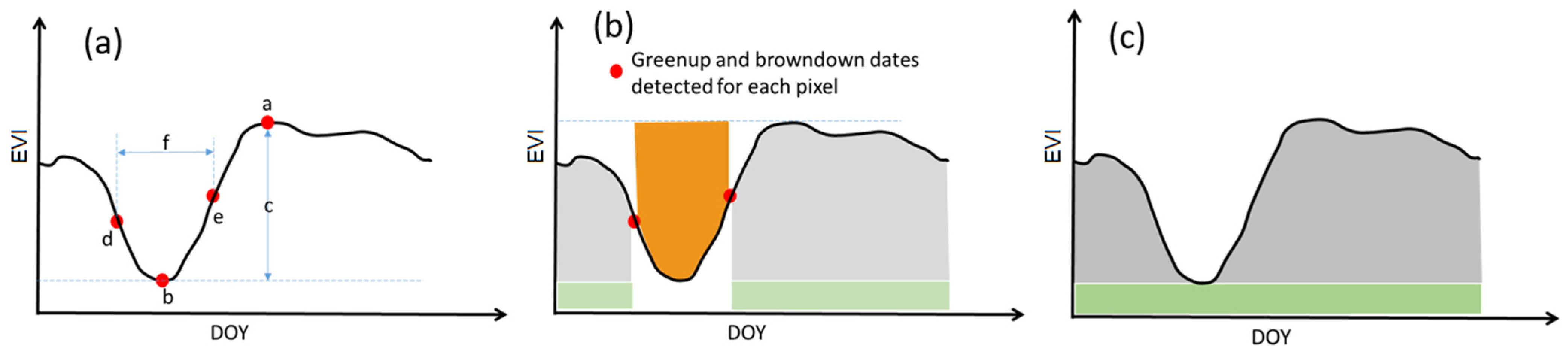
| No. | Name | Description | Unit | Definition in EVI Time Series in Figure 6 |
|---|---|---|---|---|
| 1 | Maximum EVI | Largest EVI value | EVI unit | a in Figure 6a |
| 2 | Minimum EVI | smallest EVI value | EVI unit | b in Figure 6a |
| 3 | Amplitude | Difference between the maximum and minimum EVI | EVI unit | c in Figure 6a |
| 4 | Peak Date | Date of the largest EVI | Day from 1 January | a in Figure 6a |
| 5 | Lowest Date | Date of the smallest EVI | Day from 1 January | b in Figure 6a |
| 6 | Greenup Rate | Linear slope of EVI increase during the greenup process | EVI unit/day | Slope from b to e in Figure 6a |
| 7 | Browndown Rate | Linear slope of EVI decrease during the browndown process | EVI unit/day | Slope from d to b in Figure 6a |
| 8 | Greenup Date | Date when the EVI increases to 50% during the greenup process | Day from 1 January | e in Figure 6a |
| 9 | Browndown Date | Date when the EVI decreases to 50% during the browndown process | Day from 1 January | d in Figure 6a |
| 10 | Dry season length | Time interval between browndown and greenup dates | Days | f in Figure 6a |
| 11 | Small Integral over growing season | Integral over growing season of each pixel giving area between the curve and minimum EVI value | EVI unit × day | Light Gray shaded area in Figure 6b |
| 12 | Large Integral over growing season | Integral over growing season of each pixel giving area between the curve and 0 | EVI unit × day | Light gray and light green shaded area in Figure 6b |
| 13 | Integral over dry season | Integral of EVI values over the main dry season of each pixel | EVI unit × day | Orange shaded area in Figure 6b |
| 14 | Small Integral over the whole year | Integral of EVI values above the minimum EVI over whole year | EVI unit × day | Gray shaded area in Figure 6c |
| 15 | Large Integral over the whole year | Integral of EVI values over whole year | EVI unit × day | Gray and green shaded area in Figure 6c |
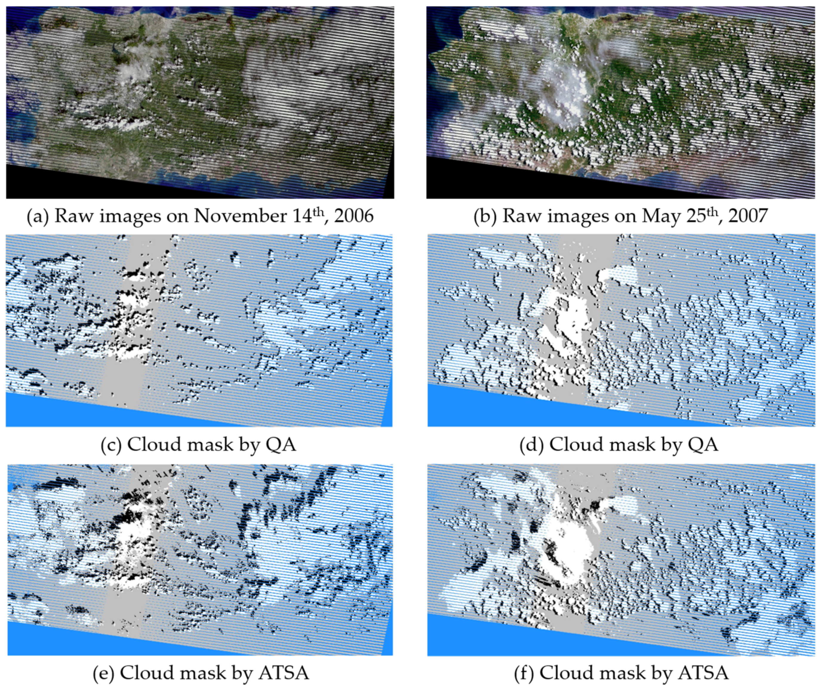
| Images | Cloud Masks | Cloud | Cloud Shadow | |||
|---|---|---|---|---|---|---|
| oa | ua | pa | ua | pa | ||
| 14 November 2006 | QA band | 0.747 | 0.931 | 0.593 | 0.334 | 0.223 |
| ATSA | 0.958 | 0.997 | 0.917 | 0.920 | 0.935 | |
| 25 May 2007 | QA band | 0.827 | 0.831 | 0.811 | 0.520 | 0.441 |
| ATSA | 0.973 | 0.988 | 0.963 | 0.895 | 0.951 | |
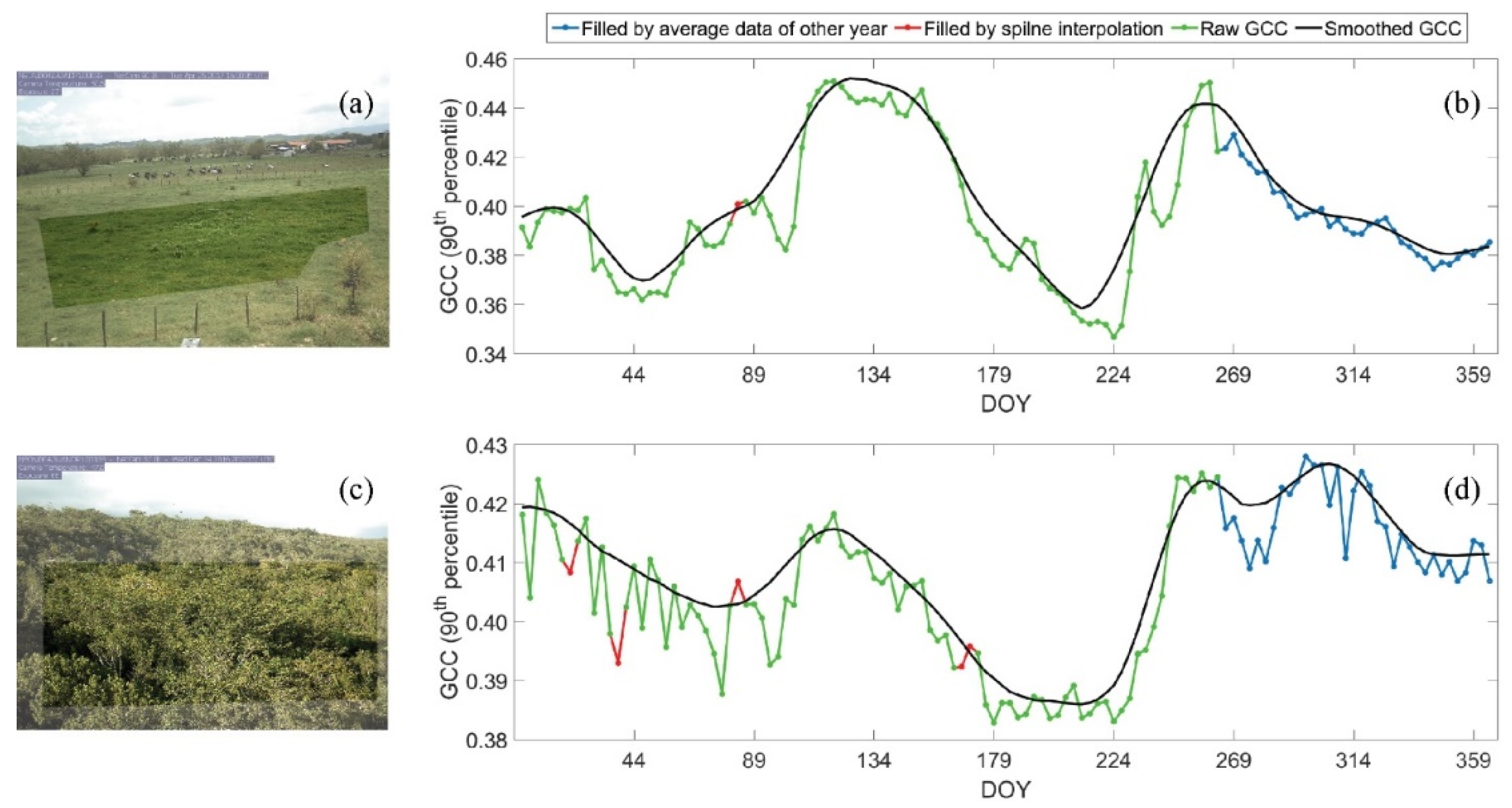
| PhenoCam A | PhenoCam B | |||
|---|---|---|---|---|
| Phenology Metric | GCC | EVI | GCC | EVI |
| Peak Date | 126 | 143 | 304 | 306 |
| Lowest Date | 213 | 201 | 212 | 229 |
| Greenup Date | 234 | 247 | 238 | 264 |
| Browndown Date | 171 | 168 | 159 | 82 |
| Dry season length | 64 | 80 | 80 | 183 |
Publisher’s Note: MDPI stays neutral with regard to jurisdictional claims in published maps and institutional affiliations. |
© 2021 by the authors. Licensee MDPI, Basel, Switzerland. This article is an open access article distributed under the terms and conditions of the Creative Commons Attribution (CC BY) license (https://creativecommons.org/licenses/by/4.0/).
Share and Cite
Zhu, X.; Helmer, E.H.; Gwenzi, D.; Collin, M.; Fleming, S.; Tian, J.; Marcano-Vega, H.; Meléndez-Ackerman, E.J.; Zimmerman, J.K. Characterization of Dry-Season Phenology in Tropical Forests by Reconstructing Cloud-Free Landsat Time Series. Remote Sens. 2021, 13, 4736. https://0-doi-org.brum.beds.ac.uk/10.3390/rs13234736
Zhu X, Helmer EH, Gwenzi D, Collin M, Fleming S, Tian J, Marcano-Vega H, Meléndez-Ackerman EJ, Zimmerman JK. Characterization of Dry-Season Phenology in Tropical Forests by Reconstructing Cloud-Free Landsat Time Series. Remote Sensing. 2021; 13(23):4736. https://0-doi-org.brum.beds.ac.uk/10.3390/rs13234736
Chicago/Turabian StyleZhu, Xiaolin, Eileen H. Helmer, David Gwenzi, Melissa Collin, Sean Fleming, Jiaqi Tian, Humfredo Marcano-Vega, Elvia J. Meléndez-Ackerman, and Jess K. Zimmerman. 2021. "Characterization of Dry-Season Phenology in Tropical Forests by Reconstructing Cloud-Free Landsat Time Series" Remote Sensing 13, no. 23: 4736. https://0-doi-org.brum.beds.ac.uk/10.3390/rs13234736