Assessing the Utility of Sentinel-1 Coherence Time Series for Temperate and Tropical Forest Mapping

Abstract

This study tested the ability of Sentinel-1 C-band to separate forest from other common land use classes (i.e., urban, low vegetation and water) at two different sites. The first site is characterized by temperate forests and rough terrain while the second by tropical forest and near-flat terrain. We trained a support vector machine classifier using increasing feature sets starting from annual backscatter statistics (average, standard deviation) and adding long-term coherence (i.e., coherence estimate for two acquisitions with a large time difference), as well as short-term (six to twelve days) coherence statistics from annual time series. Classification accuracies using all feature sets was high (>92% overall accuracy). For temperate forests the overall accuracy improved by up to 5% when coherence features were added: long-term coherence reduced misclassification of forest as urban, whereas short-term coherence statistics reduced the misclassification of low vegetation as forest. Classification accuracy for tropical forests showed little differences across feature sets, as the annual backscatter statistics sufficed to separate forest from low vegetation, the other dominant land cover. Our results show the importance of coherence for forest classification over rough terrain, where forest omission error was reduced up to 11%.

1. Introduction

Forest ecosystems host a large portion of terrestrial biodiversity, and provide many ecosystem services, such as timber and food production, risk mitigation (i.e., flood, erosion), and climate regulation, as forests hold a large portion of terrestrial biomass, and its growth and degradation play an essential role on climate and atmospheric CO₂ dynamics. This has prompted several international agreements to preserve forest services and biodiversity, along with specific procedures to track forest cover and status. One of the earliest international efforts for tracking forest status was undertaken under the Food and Agriculture Organization (FAO) through the global Forest Resources Assessment (FRA), whose first report was published in 1948. FRA defines forest as areas with tree canopy cover above 10%, 5 m minimum tree height, and a minimum extent of 0.5 Ha [1].

Forests’ increasing importance is reflected by subsequent conventions such as the United Nations (UN) Rio Convention on Biological Diversity [2], and the UN Framework Convention on Climate Change [3], UNFCC. The UNFCC was extended by the Kyoto protocol and the Paris agreements [4,5] with the commitment of the signatory countries to reduce their greenhouse gasses emissions through, among other, reforestation programs. Further forest-related agreements include the Bonn Challenge [6], a global effort for forest restoration, and the New York declaration of forests [7], aimed at reducing the rate of deforestation. Agreements under the UNFCC use indicators considered critical to characterize Earth’s climate, the so called essential climate variables (ECVs) [8] which are assessed and monitored through a range of programs and frameworks to track compliance. For example, between 2005 and 2015 the UN funded the REDD+ program, focused on “Reducing emissions from deforestation and forest degradation and the role of conservation, sustainable management of forests and enhancement of forest carbon stocks in developing countries” [9]. REDD+ requires the implementation of measurement, reporting and verification (MRV) systems as part of developing national forest monitoring systems. In the context of MRV systems, remote sensing technologies were used to keep track of forest status thanks to the short revisit times and consistent large-scale coverage.

Currently, most forest related ECVs are retrieved from earth observation satellites, with the European Space Agency (ESA) Climate Change Initiative (CCI) funding the extraction of many forest-related variables (i.e., land cover, above ground biomass, burned area) along with other ECVs (i.e., aerosols, sea surface temperature, snow cover, etc.). Remote sensing is the only technology able to provide the short revisit times and large-scale coverage needed for such tasks [10]. Recent approaches on forest/non-forest (FNF) classification leveraged optical imagery from AVHRR, MODIS, MERIS or Landsat, despite the cloud cover related problems of such sensors [10,11,12,13,14]. Active systems such as space-borne light detection and ranging (LiDAR) are sensitive to forest height and fractional cover, which are important indicators for separating forested areas [1]. However, the use of space-borne LiDAR is limited by its sparse coverage and cloud cover as is the case for the global ecosystem dynamics investigation (GEDI) instrument onboard the international space station [15]. Active systems based on synthetic aperture radar (SAR), are not affected by cloud cover, provide continuous or near continuous coverage (due to distortions over rough terrain), and are sensitive to forest presence [10,12,16].

Over the past decades, the SAR backscatter coefficient has been employed for many forest-mapping studies [10,11,17,18]. Forests tend to have higher backscatter coefficient than other land cover classes due to the multiple bounces of the signal within the canopy (volume scattering), allowing a larger amount of energy to return to the sensor. In general, longer wavelengths provide a larger contrast between forest and other classes [11,19] while cross-polarized channels are better suited at identifying forest cover since multiple bounces within the canopy cause the return to lose its original polarization [20,21]. Recent mapping examples include the ALOS PALSAR forest/non-forest maps [11] which used L-band HV (horizontal (H) transmit—vertical (V) receive) backscatter to determine forest extent, while water bodies and non-forest areas are separated using the HH channel.

The utility of the backscatter coefficient for land cover mapping is often limited by unrelated factors such as dielectric (i.e., soil moisture) and geometric effects (i.e., roughness, tree stumps and debris left after forest clearing) as well as rain, snow, and freeze-thaw periods [10,11,13,16,22,23]. For example, the backscatter coefficient may increase after forest clearing, as tree stumps and woody debris are left exposed (double bounce) and decrease with time as soil surface dries [11]. Furthermore, some land cover classes may be misclassified due to their scattering properties’ similarity to those of forest cover (i.e., vineyards, urban parks, and gardens). Nevertheless, changes in backscatter may be employed for detecting changes in the land cover (e.g., forest loss) [24,25].

Phase information may be leveraged for land cover classification to avoid the shortcomings of backscattering intensity, albeit at the cost of increased data volumes and processing times. Single-pass interferometry has been successfully applied to generate a global forest map based on TanDEM-X HH interferometric coherence, i.e., the correlation between images acquired from different sensor positions acquired at the same time (single-pass) or at different time steps (repeat–pass) [13]. Repeat–pass interferometric coherence has been also employed for land cover classification [14,26,27,28,29] with shorter temporal baselines improving the contrast between classes [28,29]. Nevertheless, such contrast may be lost over some land cover classes (e.g., crops due to tillage) even for images acquired at very short intervals [28,29]. Using dense time series (6–12 days) may overcome such limitations, but at a steep increase of data volume. Alternatively, adding coherence estimates from a few pairs with long temporal baselines can improve separating some classes, such as urban cover, ref. [14] with a smaller computational cost.

Regardless of whether phase information has been employed, multitemporal datasets may inform classifiers on land cover temporal behavior. This information can be leveraged in several ways, such as using individual observations as features, or using the pixel-wise annual statistics (i.e., average, standard deviation). When both approaches were tested in the context of forest mapping, the latter approach obtained improved results [10], as it reduces data dimensionality and it is less vulnerable to the influence of short-lived events such as precipitation [10,14,17]. However, it is important to note that the usefulness of such statistics may be hampered by variability due to thawing/flooding events or infrequent image acquisition [16]. Within annual statistics layers, SAR backscatter variations are usually lower over forested areas when compared to other land cover classes such as crops which are affected by cultivation cycles [10,17]. Forest limited annual variation is related to scattering from tree canopy and the associated dampening of temporal variations in soil surface moisture. However, annual variations may not suffice when separating younger forests as the scattering is influenced by the underlying soil properties [17], or in areas with pronounced seasonality [10]. Urban areas may also be misclassified as forests, as they have a similarly low variability. Hence, the annual backscatter average is also needed to separate forest from urban areas (infrastructure has a high backscatter coefficient [17]).

The objective of this study was to investigate the contribution of radar backscatter and coherence for forest cover mapping in temperate and tropical settings. Three increasingly richer feature sets were employed to assess the contribution of the variables that separate forest from other major land classes such as urban, low vegetation, and water. The first feature set was derived from annual backscatter statistics, the second set included long-term coherence (i.e., coherence estimate for two acquisitions with a large time difference) while for the last set short-term coherence statistics were added (i.e., average and standard deviation of coherence estimates with a short temporal baseline). The results were assessed using existing land cover datasets and spaceborne Lidar data.

2. Study Area and Data Employed

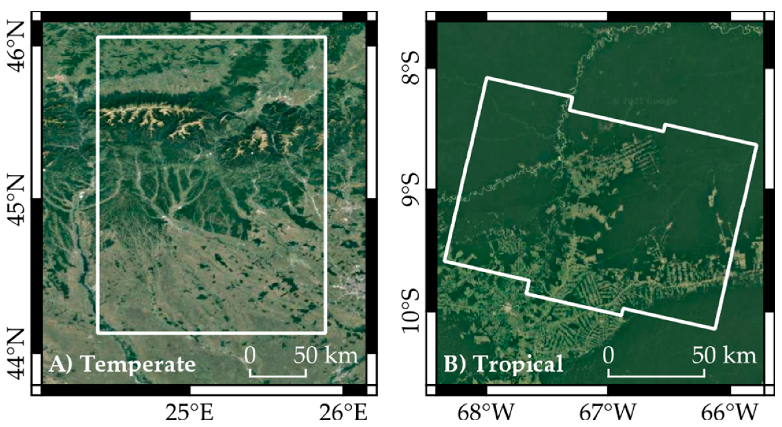
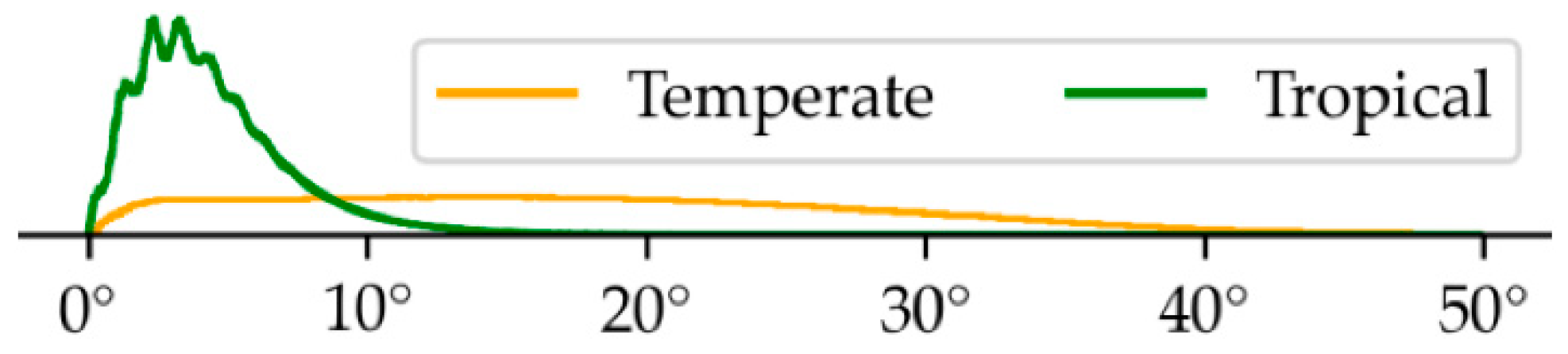
The first study area (Figure 1A) was a N-S transect over the Romanian Carpathians characterized by continuous and discontinuous urban areas, water courses and water bodies, croplands, tree and bush orchards, herbaceous cover (natural grasslands and pastures), as well as broadleaf, needleleaf and mixed temperate forest. Forests appear mainly on over-sloped terrain (Figure 2). It has an approximate area of 25,000 km². The second study area (Figure 1B) was in the Brazilian Amazon. It mainly contains broadleaf tropical forest and cropland mixed with natural vegetation (tree, shrub, herbaceous), with several water courses and small cities. At this site, forests appear mainly over gentle slopes (Figure 2). It has an approximate area of 43,000 km².

Dual-polarized (VV, VH) single look complex (SLC) images acquired by Sentinel-1 A and B satellites (C-band) in interferometric wide swath mode (IWS) were used. The SLC images have a pixel spacing of 14.1 m in azimuth and 2.3 m in range. At the temperate site (Romania), we processed all overlapping acquisitions (6-day repeat interval) from both, ascending (29, 131) and descending (7) “orbital tracks” for years 2017–2019 to ensure complete coverage of the rough Carpathians terrain. Data from these three orbits were normalized (geometric, radiometric, interferometric) using the 12 m TanDEM-X digital elevation model (DEM) [30] (©DLR, Deutsches Zentrum für Luft- und Raumfahrt 2019). For the tropical site (Brazil) we processed a time series for years 2018 and 2019, including only images from Sentinel-1A (12-day repeat interval) to ensure coherence observations with the same temporal baseline. Notice that Sentinel-1B satellite started to consistently acquire images over the area after May 2019. For the flatter terrain at the tropical site, the use of data from one relative orbit (54) was considered sufficient. SAR processing at this site was based on the NASADEM height data [31,32].

We used preexisting land cover maps as data sources to generate a consistent layer for training and validation purposes including:

• 2018 Corine land cover (CLC), generated by manual digitalization over satellite imagery with a minimum polygon area of 25 hectares [33,34], with an overall accuracy of 88.7% within the boundaries of Romania [35].
• 2015 European Space Agency Climate Change Initiative land cover dataset (ESA CCI LC, from here on CCILC), generated at 300 m resolution with a time series of optical data (AVHRR, MERIS, SPOT-VGT, POBA-V) and machine learning [36], with an accuracy of 75.1% [37].
• 2016 global urban footprint (GUF), generated at 12 m resolution with texture and intensity of TanDEM-X imagery, with an accuracy of 85–88% [38].
• 2011–2015 TanDEM-X forest non-forest map (TFNF), generated with 50 m resolution from TanDEM-X bistatic coherence data, with an estimated accuracy of 85–93% [13].
• 2017 Advanced land observing satellite phased array type L-band synthetic aperture radar forest/non-forest map (ALOS PALSAR FNF, shortened to AFNF) generated at 25 m resolution using backscatter data, with an accuracy of 85–95% [11].

To account for possible changes after the creation of the mentioned land cover datasets, we used the GEDI level 2B data from period 20/04/2019–15/04/2020 (both sites) and one Sentinel-2 image (tropical site, tiles 19LEK, 19LEL, 19LFK, 19LFL, 19LGK, 19LGL) acquired 24 August 2020.

3. Methods

3.1. SAR Data Processing

Before SAR data processing, the DEMs employed for SAR co-registration and radiometric/geometric corrections were mosaicked. Both the TanDEM-X DEM and the NASADEM tiles were received in equiangular coordinates. The TanDEM-X DEM, received as height above the ellipsoid with 12 m pixel spacing, was mosaiced and resampled to 20 m using bilinear interpolation. The NASADEM, received with a pixel size of 30 m and geoidal height reference, was mosaiced and shifted to ellipsoidal heights.

The Sentinel-1 SLC sub-swathes were assembled into a single image and multi-looked to a pixel spacing of approximately 25 m, using a factor of 7 in range, and 2 in azimuth. This allowed reducing the impact of speckle while bringing the pixel size closer to the resolution intended for analysis. The first image acquired in each relative orbit served as master. All remaining acquisitions were co-registered, by relative orbit, to the master image using an iterative process based on intensity matching and spectral diversity with the DEM as auxiliary dataset [39]. The DEM was employed to generate a lookup-table (LUT), relating its own coordinates (map coordinates) and the SAR image coordinates (range-doppler coordinates), as well as auxiliary layers containing information on terrain slope and orientation, local incidence angle, scattering area and layover and shadowed areas. Interferograms were generated between subsequent image pairs as well as at yearly intervals starting with the master image acquisition date. Two series of interferograms were thus obtained for each relative orbit: (1) the long-term series containing two to three yearly estimates, and (2) the short-term series containing near weekly (6 days) or bi-weekly (12 days) estimates depending on the study area. The topographic phase was subsequently removed and coherence was estimated for each interferogram using a two-step adaptive approach [40,41].

The backscatter intensity was calibrated to terrain flattened γ⁰, considering the incidence angle and the terrain scattering area estimate [42,43,44]. A multi-temporal speckle filter was applied to reduce speckle [17]. Coherence and backscattering intensity estimates were orthorectified using an inverse distance resampling and the yearly average and standard deviation (SD) were computed for each SAR metric (VV and VH backscatter and VV coherence) and converted to the decibel (dB) scale.

Notice that layover and shadow areas were masked using the DEM-derived auxiliary layers. Foreshortened areas were also masked, because scattering area may be underestimated, leaving them with anomalously high values. To determine when such anomalies appear, we characterized the distribution of the annual average of VH backscatter, calculating its median and median absolute deviation for all forest pixels (forest was expected to have the largest values over sloping terrain). A pixel was marked as distorted if the mean annual VH backscatter had a median-based z-score larger than 3 in all years and the pixel was within 100 m of any LUT-masked pixel (i.e., pixels where topographic normalization may still be problematic).

3.2. Land Cover Reference Dataset

We used two datasets for training and validation: a GEDI-derived point layer showing forest cover presence or absence, and a land cover raster layer. For the GEDI-based layer, shots (points) were labeled as presence when the fractional tree cover was above 10%, as estimated from both the GEDI shots and the Landsat-derived tree cover ancillary data included in the GEDI file; the canopy height (rh100) was above 5 m. If none of these thresholds was reached, the shot was considered as non-forest.

The land cover dataset was created by a Boolean combination of preexisting land cover maps. To combine them, we first resampled all data sources to a pixel grid matching the Sentinel-1 dataset. Nearest neighbor resampling was employed for qualitative datasets, bilinear resampling was employed for Sentinel-2 data, and mode resampling was employed for GUF, as its pixel size was smaller when compared to the processed Sentinel-1 data. The matching grids were combined based on the rules depicted on the

Table 1. Temperate site classification scheme together with the ruleset employed to determine the membership based on the preexisting datasets. The subclasses are based on agreement between CLC and CCI LC. GUF had to be 255 (urban) for the homonymous class, and 0 (other) for the rest of classes. “!=” denotes the NOT operator, i.e. “!=1” indicates not classified as forest in AFNF or TFNF.

Class	Subclass	CLC 2018	CCI LC 2015	AFNF 2017	TFNF 2018
Urban	Artificial	1xx: Artificial surfaces	190: Urban areas	-	0: Urban
Low vegetation	Crops	211: Non-irrigated Arable land	10: Cropland 11: Herbaceous	!=1: Other (not forest)	2: Not forest
	Pasture	231: Pastures	11: Herbaceous 130: Grassland
	Grassland	321: Grassland
	Permanent crops	222: orchards 242: agriculture mix	12: Tree or shrub
	Transitional woodland-shrub	324: transitional Woodland-shrub	40–153: natural vegetation	-
Forest	Broadleaf	311: broadleaf	50–62: broadleaf	1: Forest	1: Forest
	Needleleaf	312: needleleaf	70–82: needleleaf
	Mixed	313: mixed	90: mixed
Water	Water	-	210: Water	!=1: Other	!=1: Other

and

Table 2. Tropical site classification scheme together with the ruleset employed to determine the membership based on the preexisting datasets. The subclasses are based on CCI LC. GUF had to be 255 (urban) for the homonymous class, and 0 (other) for the rest of classes. “!=” denotes the NOT operator.

Class	Subclass, CCI LC 2015	AFNF 2017	TFNF 2018	Sentinel-1 2018, 2019	Sentinel-2 2020
Urban	190: Urban areas	!=1: Other	0: Urban	-	NDVI < 0.6 NDWI < 0
Low vegetation	30: Mosaic of cropland with natural vegetation		2: Not forest	VV < −8	NDMI < 0.05 NDVI < 0.6 NDWI < 0
	40: Mosaic of natural vegetation with cropland
	100: Mosaic tree/shrub and herbaceous
	120: Shrubland
Forest	50–62: broadleaf	1: Forest	1: Forest	-	NDVI > 0.6 NDWI < 0
Water	210: Water	!=1: Other	!=1: Other	VH < −20 dB VV < −15 dB	NDWI > 0

: to receive a specific sub-class a pixel had to meet all conditions imposed for that specific subclass. The logic behind the specific ruleset is described in the following paragraphs, as different conditions were necessary for each site due to the land cover types present and the difference in available ancillary data.

At the temperate site, the AFNF was not used to determine urban cover because it disagreed with the remaining datasets (i.e., parts of the cities were classified as forest). For the rest of non-forest classes, the condition imposed on AFNF was “NOT forest”, as open areas and water surfaces were sometimes misclassified as each other due to a similarly low backscatter. In the case of transitional woodland-shrub, it was necessary to remove AFNF or relax the condition (any natural cover of CCI land cover), as most of the plots from CLC were lost due to the large size of ESA CCI pixel size, or due to the object-based generalization of AFNF. For areas meeting the imposed conditions, a two-pixel negative buffer was applied to avoid edge effects.

At the tropical site, Sentinel-1 annual averages (by polarization) were added to avoid the shortcomings of the preexisting datasets, together with normalized difference indices (ND) derived from one Sentinel-2 image (24 August 2020). In the case of low vegetation, large areas were covered by mixed land covers (forest and low vegetation appear together) in the CCI LC. To avoid including thin tree lines in the low vegetation sample, pixels with a backscattering intensity over −8 dB on the Sentinel-1 VV annual averages, a ND moisture index (NDMI [45]) over 0.05, and ND vegetation index (NDVI [46]) over 0.6 in the Sentinel-2 image were masked out, as these characteristics indicate tree cover. Forest had to have an NDVI over 0.6 in the 2020 Sentinel-2 image to avoid including areas that may have been deforested after the creation of the land cover datasets. ND water index (NDWI [47]) had to be negative for land classes, and positive for water. Water also needed to have an annual backscattering intensity average under −15 and −20 dB for VV and VH channels to avoid errors caused by changes in the water cover. Forest and low vegetation (dominant classes) received the two-pixel negative buffer. The few pixels available for urban areas precluded such a buffer. Similarly, the sample for water cover would have been greatly reduced by a negative buffer, as it appears as thin rivers.

3.3. Training Data Preparation

The training sample was taken from unmasked SAR pixels (not affected by layover, shadow, or foreshortening) in all the relative orbits employed for the site. The training dataset was designed to withhold at least 30% of the sub-class samples for validation, taking up to 25.000 random samples from the pixels with said sub-class. In the specific case of forest sub-types, samples were taken from the GEDI-derived tree cover layer, selecting the shots overlapping with a pixel with the specific forest type.

The training data was culled by applying the local outlier factor algorithm to each individual sub-class, keeping all points that were considered inliers in all orbits and years. In the case of water cover, the median-based z-score was also employed by dropping any sample where the z-score for the VH channel was over three, cases where we assumed the pixel may be partially occupied by land and/or aquatic vegetation, thus reducing the separability with low vegetation classes. For each land cover, 5000 random points evenly distributed between its subclasses were selected. All sub-classes always had over 1000 training samples, with the lowest counts for the temperate site low vegetation sub-classes (1000 samples each), and tropical site urban (1891 samples as the single sub-class). Training data was employed to plot the distribution of the land cover classes.

3.4. Classification Scheme

Yearly classifications were created using an increasing number of features. The first set includes backscatter annual statistics, the second adds long-term interferometric coherence, and the third adds short-term coherence statistics. While training the classifier, each year was considered an independent sample, i.e., each classifier was trained with 20.000 samples per year. A “one-versus-rest” linear support vector machine classifier was fitted for every orbit, as anisotropic effects may remain even after performing radiometric terrain flattening [42]. These classifiers were fit with a regularization parameter of 1, primal problem optimization, L1 penalty, 0.001 stopping tolerance, and 10.000 iterations maximum. At the temperate site, data from several relative orbits were combined to maximize coverage as large areas were masked in each individual orbit due to the SAR related geometric distortions. For each pixel, every orbit casts a vote with a weight equal to the inverse of its scattering area, as pixels with large scattering suffer larger geometric and radiometric distortions [43,48]. The pixel is classified as the land cover accumulating the largest weight. Detailed information about the methodology can be found in [49].

3.5. Validation

The land cover validation set was created after discarding pixels overlapping the GEDI shots, those that have been masked as distorted in all orbits, and any pixel that has been considered for inclusion in the training sample. The GEDI validation set (forest and non-forest classes) was created using all shots, except for those considered as candidates for inclusion in the training sample (see Section 3.2 and Section 3.3).

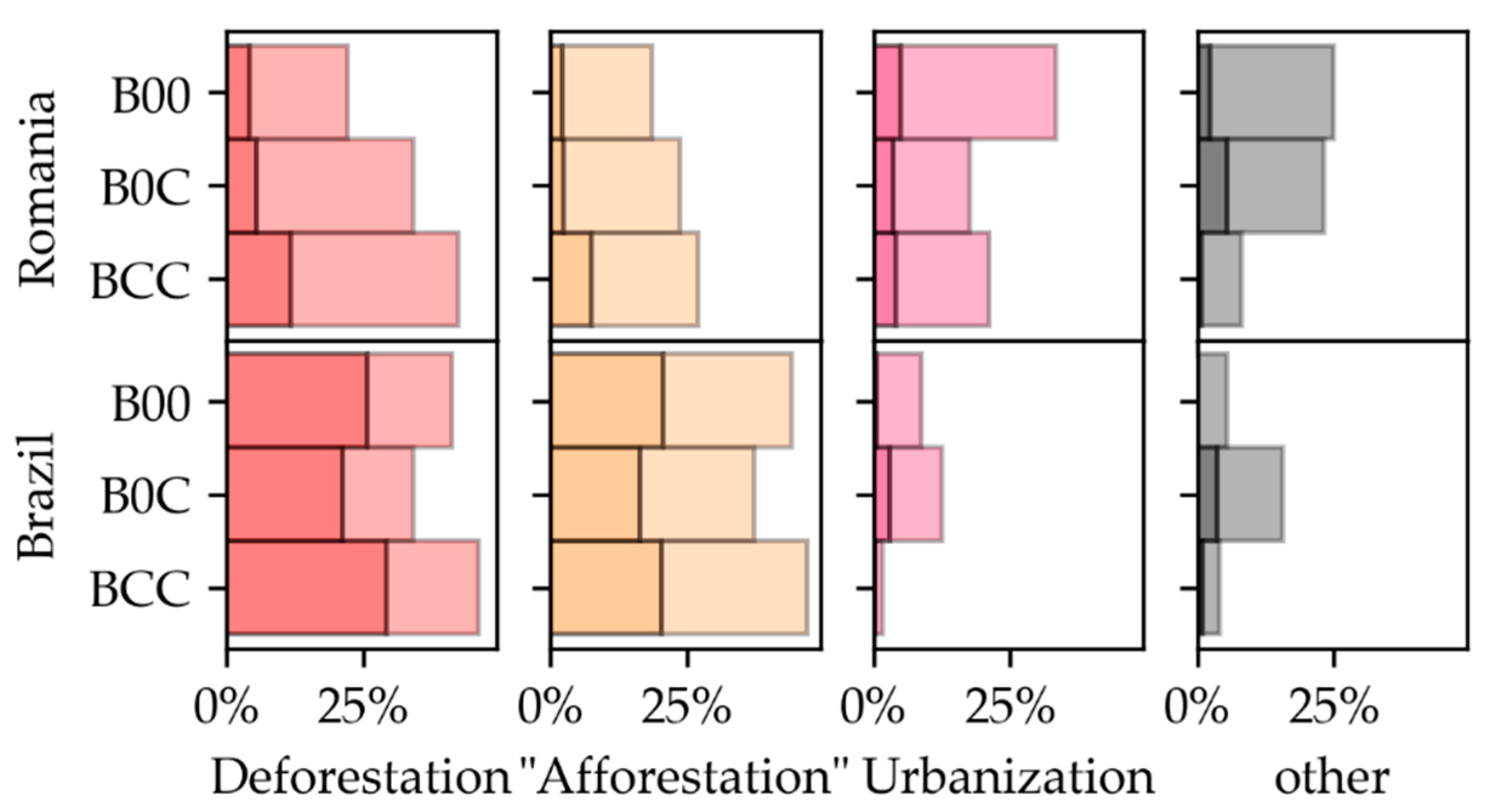
Validation was performed directly for the land cover dataset (same classes), whereas, for comparison with the GEDI forest/non-forest validation set, the resulting classification was matched to the GEDI binary scheme, with forests being considered as forest presence and the remaining classes forest absence. We employed confusion matrices and its derived metrics, overall accuracy (OA), Kappa statistic (K), omission, and commission errors (OE, CE) to assess the results. Alluvial diagrams were employed to track OE and CE origin. Classification stability was assessed as the percentage of unchanged pixels between yearly classifications (i.e., 2018 vs. 2019) by separating pixels with known land cover (in the validation sample) and pixels not included in the validation sample. We analyzed the type of change by disaggregating into four groups: deforestation and “afforestation” (forest to low vegetation and vice versa), water related changes (water to low vegetation and vice versa), urbanization (forest or low vegetation to urban), and other changes. Note that these changes have not been independently verified.

4. Results

4.1. Data Distribution

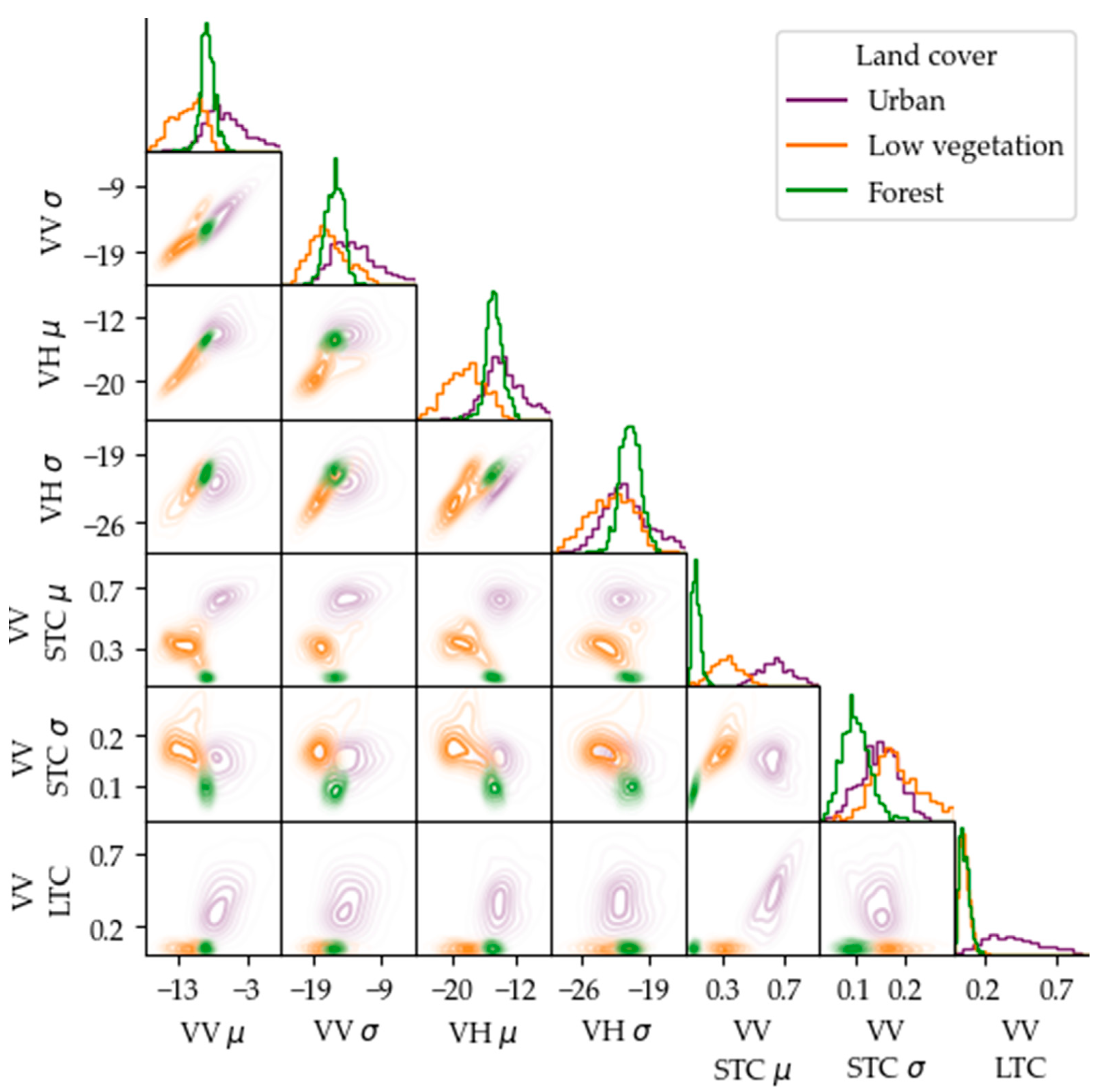
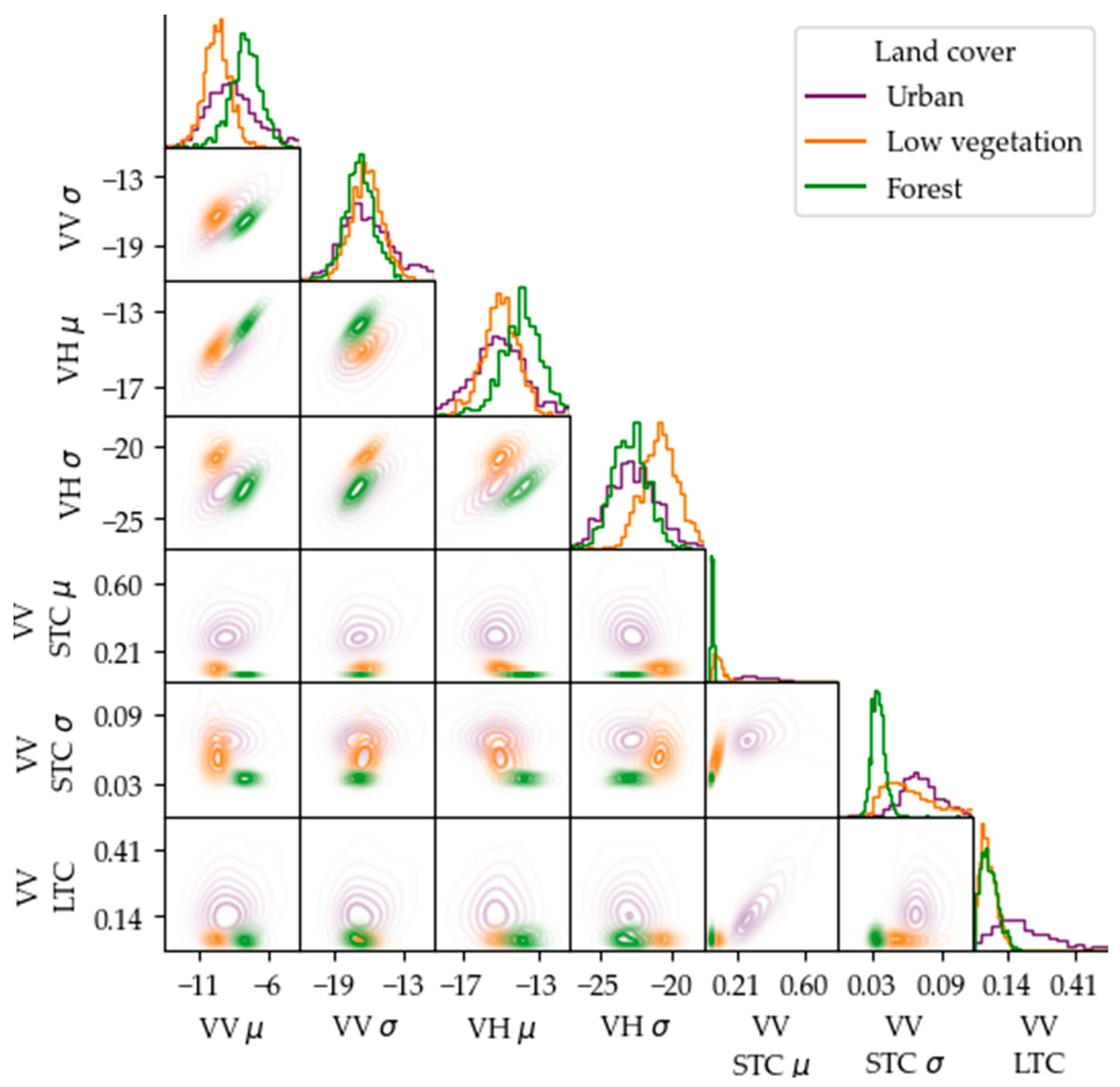
At both sites, the pixel-wise annual backscatter average was larger over forests when compared to low vegetation, with a large overlap between both. Distribution of the urban class overlapped with the distribution of the forest class, as the former showed a large variability (Figure 3 and Figure 4).

Annual backscatter standard deviation (SD) displayed similar tendencies, with a large degree of overlap between forest, low vegetation, and urban classes. Long-term coherence helped separating forests from urban, as the former generally displays lower values, with little overlap between the two classes. Average short-term coherence showed the lowest value for forest, increasing for low vegetation and reaching maximum over the urban cover. The annual standard deviation helped separating forest from low vegetation, as it tends to be higher for the latter, albeit some overlap remained.

4.2. Classification with Feature Sets

All classifications attained accurate results (OA > 90%) and substantial agreement (K > 0.75 [50]) when assessed against the reference land cover (LC) and the GEDI-derived validation sets (

Table 3. Overall accuracy (%) and kappa by classification. “LC” stands for land cover-based reference dataset. B00—classification using backscatter annual statistics, B0C—adding long-term coherence, and BCC—further adding short-term coherence statistics. Cells are shaded with a gradient between yellow and green, associated with lower, and higher metrics, respectively.

			Temperate								Tropical
		Overall accuracy				Kappa statistic				Overall accuracy				Kappa statistic
		B00	B0C	BCC		B00	B0C	BCC		B00	B0C	BCC		B00	B0C	BCC
LC	2017	94	97	99		0.86	0.93	0.98
	2018	96	97	99		0.91	0.93	0.97		98	97	99		0.87	0.85	0.92
	2019	96	97	99		0.90	0.93	0.97		99	99	99		0.93	0.91	0.96
GEDI	2017	92	96	97		0.79	0.90	0.91
	2018	93	95	96		0.84	0.89	0.91		95	95	96		0.77	0.76	0.82
	2019	93	96	96		0.82	0.89	0.90		95	95	97		0.79	0.79	0.83

). When only the backscatter annual statistics were used as predictors, the overall accuracy ranged between 94–99% (LC) and 92–97% (GEDI). At the temperate site, the Kappa statistic ranged within the 0.86–0.91 (LC) and 0.79–0.84 (GEDI) interval, whereas at the tropical site it ranged between 0.87–0.93 (LC) and 0.77–0.79 (GEDI). Adding long-term coherence data resulted in opposite results depending on the site. At the temperate site, the overall accuracy and K increased to 97% and 0.93, respectively. Conversely, at the tropical site the Kappa statistic decreased slightly, 0.85–0.91 (LC) and 0.76–0.79 (GEDI). Adding annual statistics from short-term coherence series increased the overall accuracy at both sites to 99% (using the land cover dataset as reference) and 96–97% (using the GEDI data set as reference). Similarly, the Kappa statistic increased at both sites. At the temperate site Kappa increased to 0.97–0.98 (LC), and 0.90–0.91 (GEDI), whereas at the tropical site it increased to 0.92–0.96 (LC), and 0.82–0.83 (GEDI).

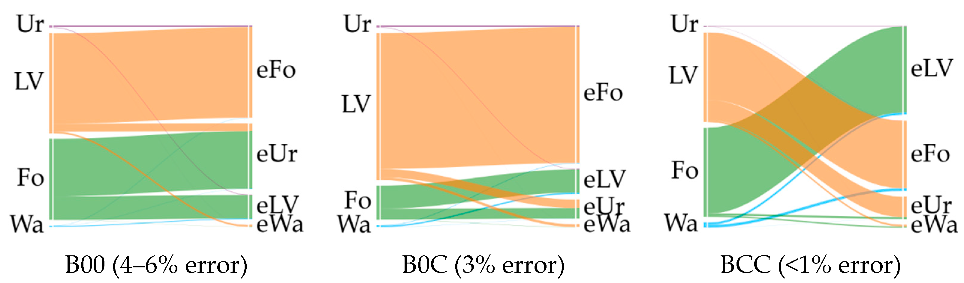
At both sites, the prevalent land cover types (low vegetation and forest) were most affected by misclassification (Figure 5 and Figure 11). However, there were different tendencies between the two study sites. At the temperate site, using only the backscatter annual statistics as predictor variables resulted in an omission error (OE) of 4–12% for the forest class, with most pixels being assigned to the urban class, which showed an 83% commission error for 2017, 60% for 2018 and 67% for 2019 (

Table 4. Temperate site errors (%) disaggregated by land cover (Ur, Urban; LV, low vegetation; Fo, forest; Wa, water). B00—classification using backscatter annual statistics, B0C—adding long-term coherence, and BCC—further adding short-term coherence statistics. Complete matrices in Appendix A (Table A1). Cells are shaded with a green-yellow gradient, indicating lower and higher errors.

		2017					2018					2019
		Ur	LV	Fo	Wa		Ur	LV	Fo	Wa		Ur	LV	Fo	Wa
Commission error	B00	83	1	9	14		60	1	8	11		67	1	8	16
	B0C	37	1	7	14		30	1	7	10		28	1	7	14
	BCC	16	<1	1	6		13	1	1	5		17	1	1	5
Omission error	B00	7	4	12	9		14	4	4	9		11	4	6	9
	B0C	4	3	2	9		4	3	2	9		6	3	2	9
	BCC	1	1	1	8		1	1	2	8		1	1	2	9

, Figure 5).

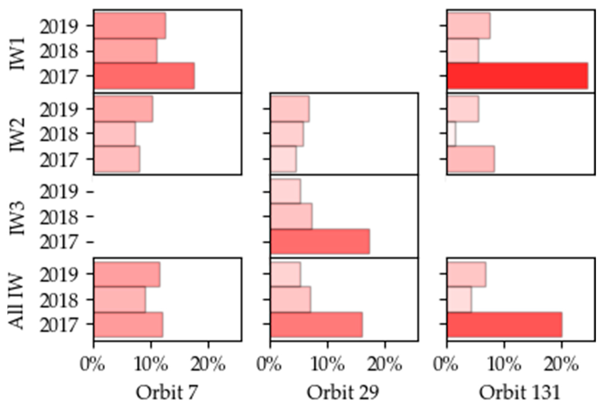
There was a large variation on urban commission error across the yearly classification, with forest being the main contributor. To understand the source of this misclassification, we examined the prevalence of said error in the individual classifications generated for each orbit disaggregating by sub-swathes (Figure 6). For the by-orbit classification of year 2017, the misclassification of forest as urban was more prevalent within a particular sub-swath for both, 29 and 131 orbits.

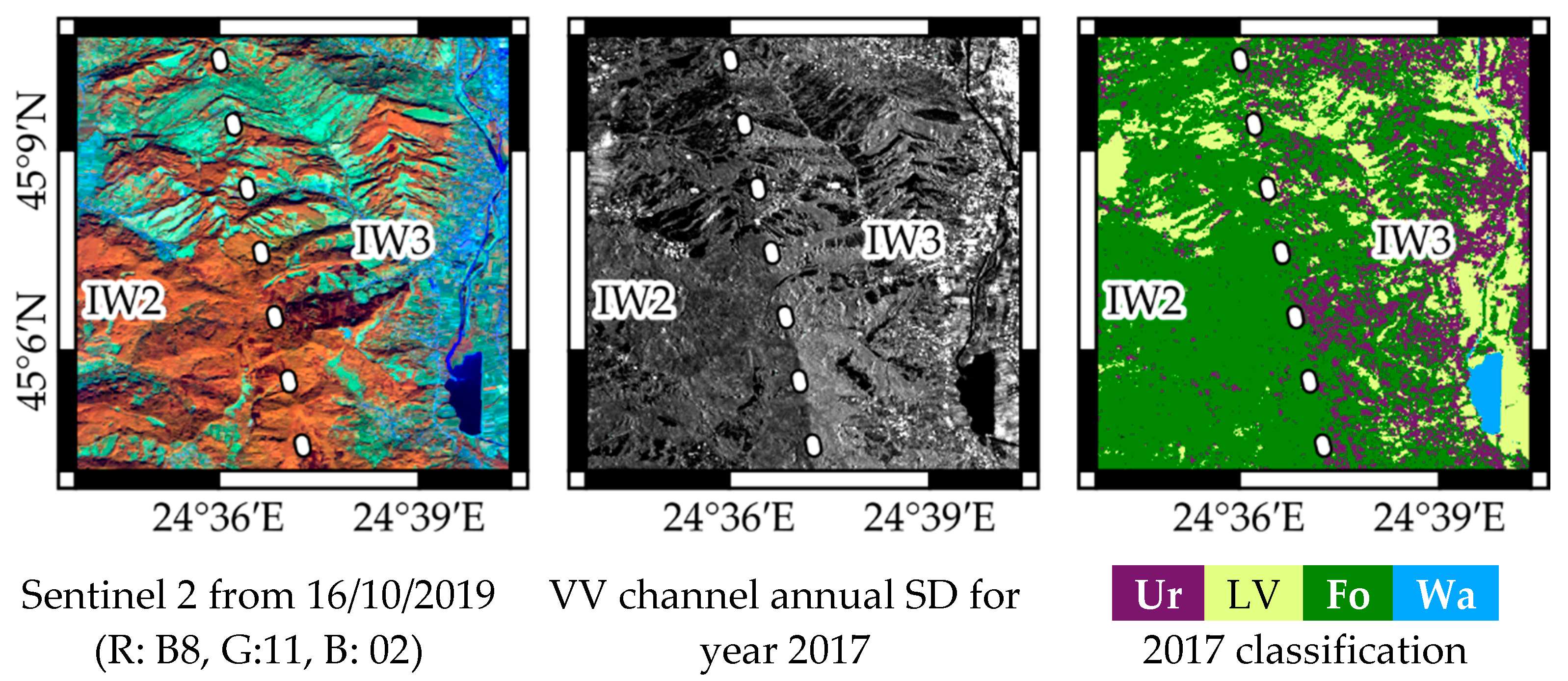
When displaying the 2017 classifications there is a clear cutline, where misclassification becomes more prevalent (Figure 7).

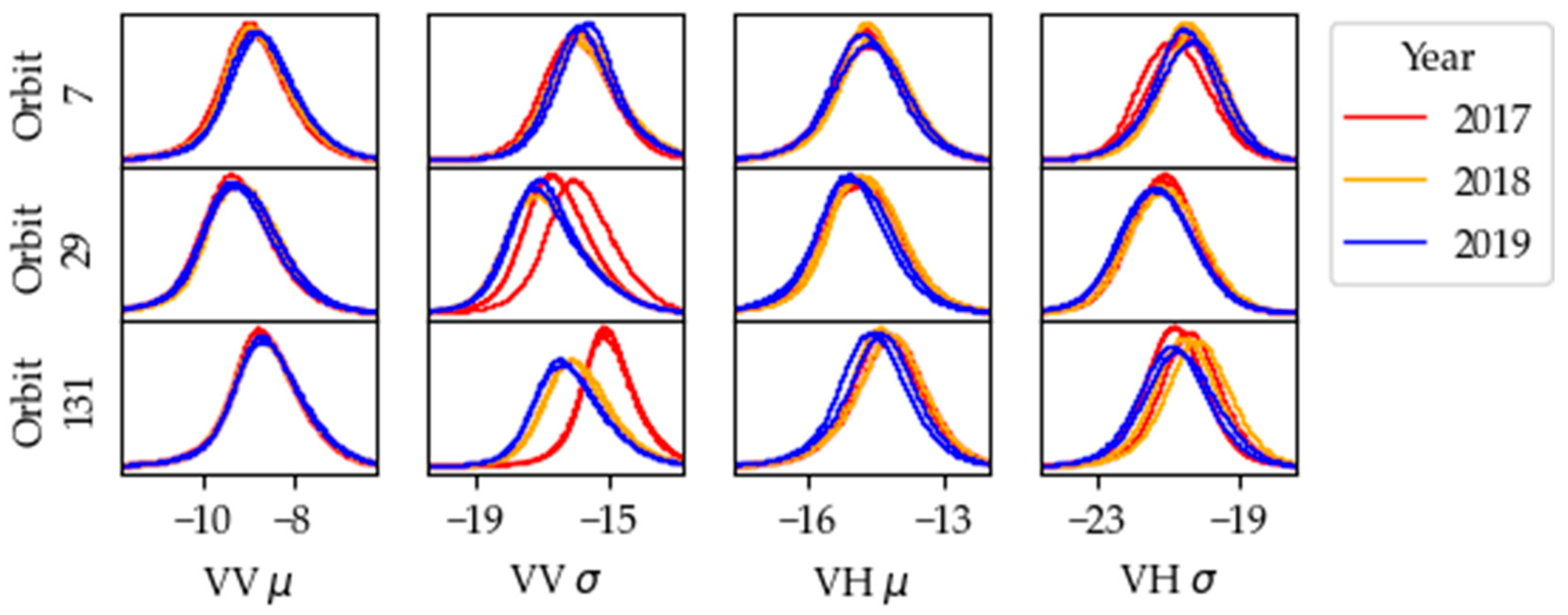
To understand the sub-swathes differences, we plotted the distribution of all pixels labeled as forest in the validation sample disaggregating by orbit, year, and sub-swath (Figure 8). VV and VH annual averages showed little difference between years and sub-swathes, with a near-complete match between the distributions of all years and sub-swathes. However, for year 2017 the VV annual SD for ascending orbits (29, 131) had its distribution shifted compared to years 2018 and 2019. For orbit 29, the distributions for the sub-swathes were centered around different values, whereas both had a similarly high value for orbit 131. VH annual SD showed smaller shifts, with some mismatch between sub-swathes from orbit 131.

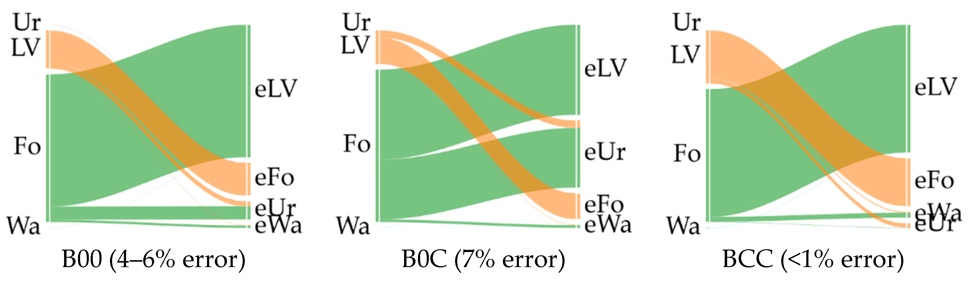
Omission errors for forest class were reduced when coherence information was included. Adding long-term coherence as predictor reduced forest OE to 2%, while urban CE decreased to 28–37%. Including coherence annual statistics further reduced the commission error for urban class (from 28–37% to 13–17%), forests (from 7% to 1%), and water (from 10–14% to 5–6%).

Evaluating forest cover presence with the GEDI-derived reference (

Table 5. Temperate site errors (%) based on GEDI forest presence/absence validation dataset. B00—classification using backscatter annual statistics, B0C—adding long-term coherence, and BCC—further adding short-term coherence statistics. Complete matrices in Appendix A (Table A2). Cells are shaded with a green-yellow gradient, indicating lower and higher errors.

		2017				2018				2019
		B00	B0C	BCC		B00	B0C	BCC		B00	B0C	BCC
Commission error	Forest	14	10	2		15	12	3		15	11	2
	Other	7	2	4		3	1	4		4	2	5
Omission error	Forest	18	5	11		8	4	11		10	4	13
	Other	5	4	1		6	5	1		6	5	1

) showed CE and OE for forest cover between 14–15% and 8–18%, respectively, when using backscatter annual statistics as predictor variables. CE and OE for non-forest ranged between 3 and 7%. Adding long term coherence reduced errors for both forest and non-forest classes whereas including coherence annual statistics further reduced CE for the forest class from 10–12% to 2–3%, while increasing OE omission from 4–5% to 11–13%. As expected, the non-forest class showed opposite trends., i.e., decreasing OE from 4–5% to 1%, and increasing CE from 1–2% to 4–5%.

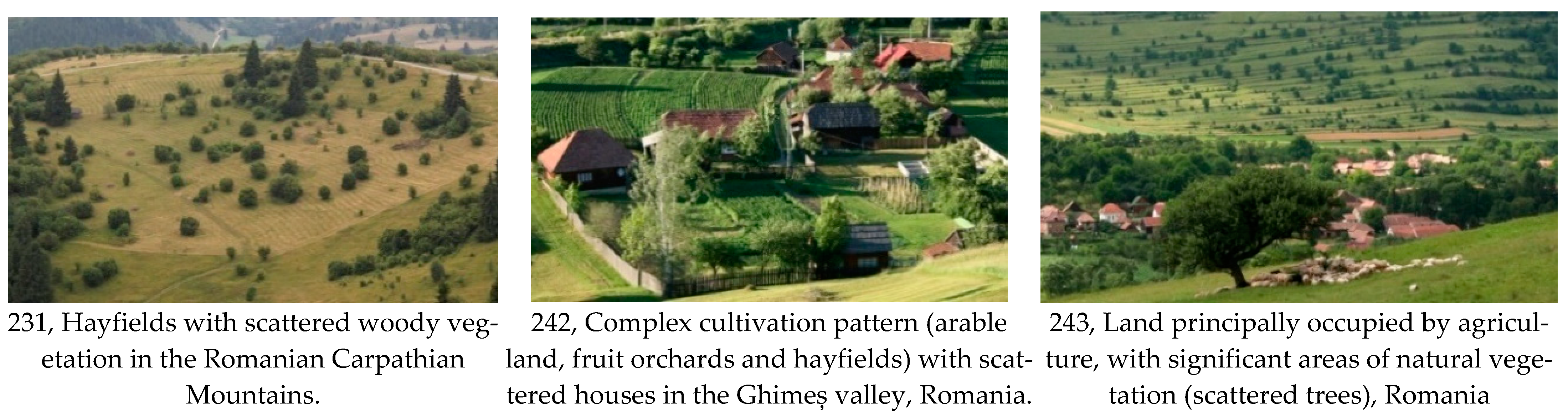
Classifications using the full feature set had opposing trends on CE and OE, depending on the validation set employed for the assessment. Such trends were explained by examining the CCI/CLC cover over the GEDI shots where forest omission had happened. Most such shots were considered broadleaf forests (27–32% CCI, 19–27% CLC) followed by the CLC classes “Fruit tree and Berry plantations”, “Complex cultivation patterns”, and “Land mainly occupied by agriculture”. Combined, these agricultural areas represented a 35–41% of OE for forest class when using the GEDI-derived reference layer. Tree and shrub were the CCI land cover class with the second largest contribution to misclassification (18–23%). Notice that CCI tree and shrub class largely corresponds to CLC agricultural classes that can have a significant tree cover (Figure 9).

For the tropical site, the overall classification errors were similar no matter the feature set employed (

Table 6. Tropical site errors (%) disaggregated by land cover (Ur, Urban; LV, low vegetation; Fo, forest; Wa, water). B00—classification using backscatter annual statistics, B0C—adding long-term coherence, and BCC—further adding short-term coherence statistics. Complete matrices in Appendix A (Table A3). Cells are shaded with a green-yellow gradient, indicating lower and higher errors.

		2018					2019
		Ur	LV	Fo	Wa		Ur	LV	Fo	Wa
Commission error	B00	99	17	<1	16		99	8	<1	16
	B0C	>99	15	<1	22		>99	6	<1	19
	BCC	89	11	<1	22		89	5	<1	17
Omission error	B00	71	4	2	1		62	4	1	1
	B0C	24	4	3	1		27	4	1	1
	BCC	7	4	1	1		9	3	<1	1

), with slight differences for the majority classes (forest and low vegetation), which increased for the minority classes, especially urban, whose omission fell from 62–71% to 7–9%. The similar classification errors may stem from the adequate separability of forest and low vegetation classes based on backscatter statistics (Figure 4).

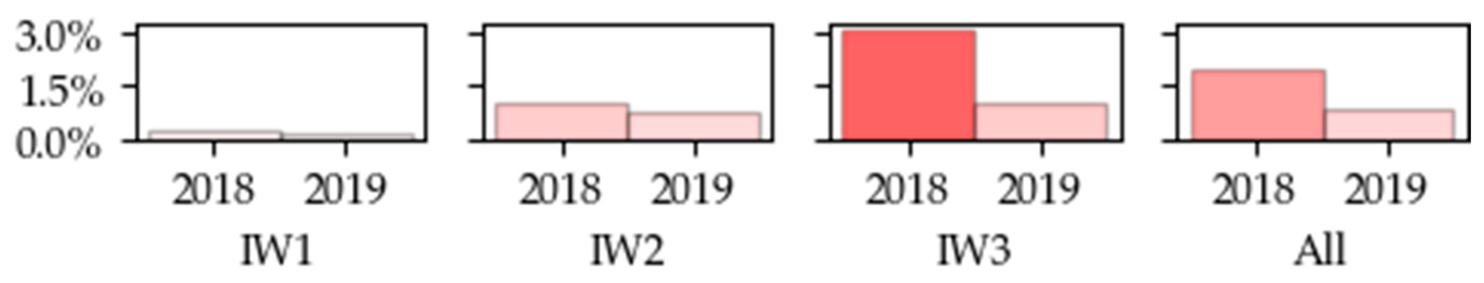
To check differences between sub-swathes on the backscatter-based classification, the percentage of forest validation pixels misclassified as low vegetation (most common misclassification of the forest class), was plotted by sub-swath (Figure 10). Indeed, a larger error (3%) was observed for sub-swath IW3 when compared to the remaining sub-swathes for year 2018. However, the differences in distribution were not as evident as at the temperate site.

At the tropical site, adding the coherence-based variables resulted in under- or over-prediction of the minority classes (Table 6, Figure 11). Adding long-term coherence reduced forest omission, low vegetation commission and urban omission errors. When coherence annual statistics were included as well, CE for low vegetation dropped to 5–11%, forest OE dropped to 1% or less, and urban CE dropped to 89%.

When assessing the tropical site classifications against the GEDI derived reference layer (

Table 7. Tropical site errors (%) based on GEDI forest presence/absence validation dataset. B00—classification using backscatter annual statistics, B0C—adding long-term coherence, and BCC—further adding short-term coherence statistics. Complete matrices in Appendix A (Table A4). Cells are shaded with a green-yellow gradient, indicating lower and higher errors.

		2018				2019
		B00	B0C	BCC		B00	B0C	BCC
Commission error	Forest	1	1	1		<1	<1	<1
	Other	32	33	25		29	29	23
Omission error	Forest	5	5	4		5	5	3
	Other	5	5	4		4	4	4

), similar results were observed regardless of the input features. Differences appeared only when short-term coherence statistics were added, with CE for non-forest dropping from 29–33% to 23–25%. In addition, the OE for both, forest and non-forest classes, were reduced by 1–2%.

4.3. Classification Stability

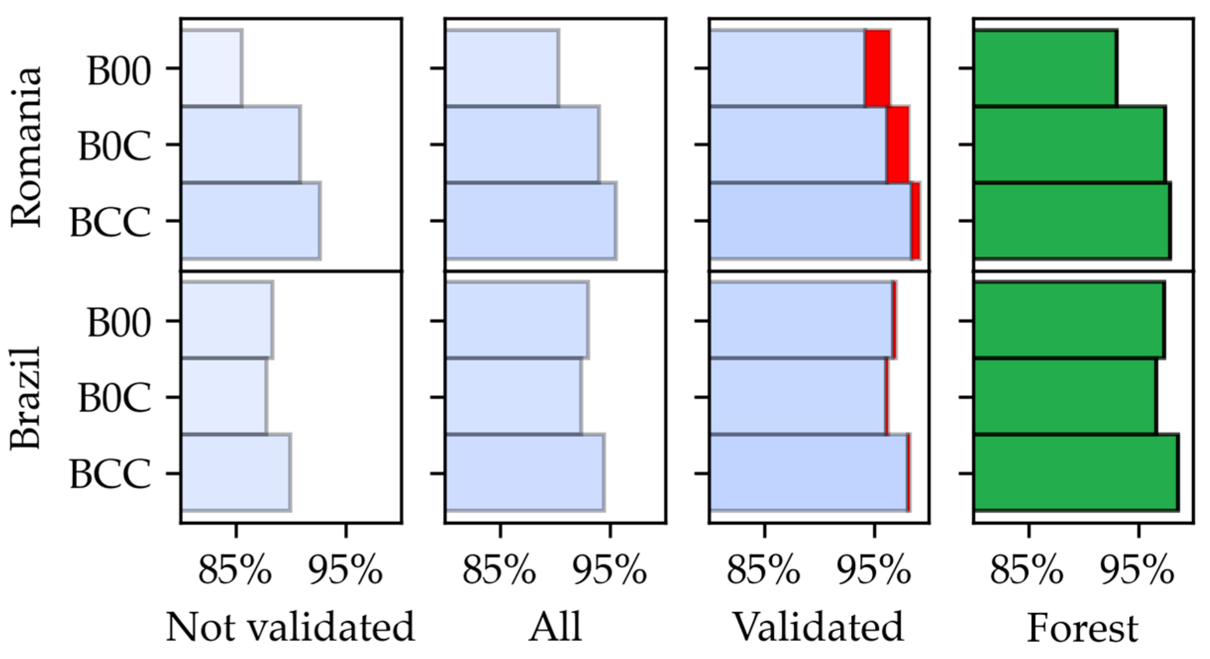
The stability between 2018 and 2019 yearly classifications was assessed. The year 2017 was excluded due to the SAR processing induced differences between sub-swaths and the lack of data over the tropical site. Over 85% of all unmasked pixels (not affected by SAR geometric distortions) were stable, i.e., did not change classes from year to year regardless of the site (Figure 12). In addition, pixels labeled as “forest” in the LC validation sample shows a particularly high stability (>95% in most cases). At the temperate site, the classification based on backscatter statistics features showed lower stability as well as slightly larger proportion of stable, but misclassified pixels when compared to classifications based on features taking advantage of the coherence information. Differences for the tropical site were smaller, with the largest stability appearing when using the full feature set, followed by the backscatter statistics set, and with little difference in the proportion of stable, but misclassified, pixels. Note that an unknown proportion of the changes detected may be actual land cover changes, as changes have not been validated.

Generally, changes between the yearly classifications (2018 vs. 2019) were caused by transitions between forest and low vegetation classes (Figure 13) which appeared frequently at class borders. At the temperate site, the apparent deforestation and afforestation increased when more coherence-based features were added, representing 41%, 58% and 70% of change as the feature set grows larger (backscatter annual statistics, long-term coherence, coherence annual statistics). These changes appeared near the mountain tops and in areas with a sparse tree cover (young forest, tree orchards). Changes from low vegetation/forest to urban accounted for 33% of the total changes. At the temperate site, unclassified changes accounted for up to 25% of all changes (using backscatter statistics), albeit most of them were eliminated by the morphological operator “opening”.

Deforestation/afforestation followed a similar trend at the tropical site, accounting for 86% of the change in the yearly classifications when using the backscatter statistics feature set, 72% when adding long-term coherence and 93% when using the full feature set. Changes from vegetation to urban and unclassified changes had a larger representation when using the full feature set, reaching 12% (compared to 2–9%) and 16% (compared to 4–5%) respectively. Nevertheless, most patches were eliminated by the “opening” operator, indicating that they appear as small, thin areas (salt and pepper noise).

5. Discussion

Backscatter-based overall mapping accuracy was high regardless of the site (OA > 92%). However, in temperate environments (i.e., Carpathians), classifications based on backscatter annual statistics frequently misclassified forest as urban, especially over steep slopes. The 2017 classification presented a particularly large tendency to misclassify forest as urban, prompting further analysis on the possible cause. The analysis showed that such misclassifications were prevalent in specific sub-swathes, where the statistical distribution of the pixel-wise annual standard deviation appears to be shifted compared to other sub-swathes and years. This phenomenon could be attributed to the limited information provided by the Sentinel-1 noise lookup table prior to 13/03/2018, which only annotated noise in the range direction. Past this date, the Sentinel-1 instrument processing facility software (IPF), was upgraded to version 2.90, and started providing noise annotations in azimuth direction as well [51,52,53]. This conclusion is also supported by the marginal differences in distribution observed for years 2018 and 2019.

Backscatter-based classifications for years 2018 and 2019 displayed a smaller tendency to misclassify forest as urban. However, misclassifications were still observed and may be related to the inclusion of 2017 data (with the related noise problem) in the training sample. Other possible sources of error were the under-correction of slopes facing the sensor [23,49,54] and the elongation of the path traversed within the forest canopy on backslopes [42]. Such errors may be alleviated if topographic information is included (orientation, slope, incidence angle, etc.) [19]. It is also important to consider that urban cover is mostly discontinuous, with a significant presence of gardens and trees that influence the urban radiometric signature (small settlements misclassified as forest), a problem that also has been encountered by [55]. Furthermore, backscatter-based maps presented lower stabilities at the temperate site which may be related to differences in the meteorological conditions across the years such as the winter length (forest presents lower backscatter in freezing conditions [22,56]), or rain frequency (less contrast between land covers [57]).

Adding long-term coherence reduced the misclassification of forest as urban up to 9%. Such reductions were possible because urban was the only land cover that retained higher coherence levels over long periods [14,26]. Errors for all land covers dropped when short-term coherence statistics were added. In particular, an important reduction of low vegetation to forest misclassification was observed, as the former has higher coherence values (i.e., pastures, grasslands), or higher variations (e.g., agriculture cropping cycle) than forests which are characterized by low coherence values [27]. Accompanying these gains in accuracy, there were successive increases in classification stability. The remaining apparent changes were mainly observed between forest and low vegetation. Apparent afforestation patches appeared close to the mountain tops and may be related to how long the stable winter conditions (i.e., increased coherence) lasted every specific year [58]. Apparent deforestation generally appeared close to the edges of forest, and in areas with smaller tree cover and height. This may be related to the use of an adaptative estimator for coherence. Such estimators reduce the loss of resolution compared to a boxcar filter, albeit it may bias the coherence estimation [29]. The employed estimator combined several coherence estimates using a gaussian weighting function [40,41]. It is possible that in border areas (i.e., forest contact with pastures) the weighting may have been modified depending on the meteorologic conditions (i.e., a coherence drop due intense precipitation), affecting the annual statistics and inducing instability.

When comparing with GEDI-derived forest presence/absence, including short-term, coherence statistics decreased the commission error for forest, but increased its omission. These opposing trends were explained by the presence of other land uses with tree presence (orchards, scattered trees, treed plot borders, Figure 4) considered as forest cover, according to the criteria set for the GEDI validation dataset, but not classified as such. This suggests that it may be possible to separate agricultural classes with significant tree cover from actual forests using the Sentinel-1 coherence temporal statistics [27]. Notice that such separation based solely on backscatter features is difficult, as is also shown in previous studies [16].

Over tropical areas, smaller differences between classifications were observed. The trends were also different when compared to temperate environments. Such differences were attributed to flatter terrain and improved Sentinel-1 processing at IPF which led to a reduced impact on the training sample. The use of C-band dual-pol backscatter annual statistics provided highly accurate results, in line with results in the recent literature [10,16,23]. This contrasts with older studies based on single-pol data from the active microwave instrument (SAR) on board of the European remote sensing missions (ERS AMI-SAR), where the C-band VV backscatter could not discriminate tropical forest from other land covers [59,60,61].

Including long-term coherence as a feature slightly decreased classification accuracy as well as its stability, due the over-prediction of urban (some near-bare areas also kept a high coherence). This had little impact on GEDI validation results, indicating the over-prediction of urban cover does not come from the misclassification of forest. Adding short-term coherence statistics increased accuracy, reducing the errors for most land cover classes, regardless of validation dataset. This is thanks to the improved contrast between forest, urban and low vegetation, as also shown in prior studies based on either ERS [59,60,61] or Sentinel-1 imagery [62,63].

Differences between sites could be related to the different land cover classes, terrain characteristics, land cover dataset generation, the changes in the Sentinel-1 IPF or the lower number of acquisitions at the tropical site, where the longer temporal baseline may have degraded the contrast between classes, and thus, the value of using coherence data [28,29].

6. Conclusions

The aim of this study was to evaluate how temporal features extracted from Sentinel-1 data affect forest/non-forest classification as well as to differentiate possible misclassification sources. Increasingly richer feature sets were tested starting with annual backscatter statistics (average and standard deviation of VV and VH backscattering intensities) and adding long-term coherence as well as short-term coherence statistics. Using only backscatter derived features has advantages as they can be obtained from the ground range detected (GRD) products. Contrarily, coherence derived metrics require pairs of single-look complex images (SLC), with the associated increase in data volume and processing times. Validation was performed with a land cover dataset, and GEDI data binarized into forest presence and absence as per the FAO definitions [1].

All three feature sets provided high overall accuracies, and acceptable omission (<19%) and commission (<16%) for forested areas with additional improvements in accuracy and classification stability being observed as more features were added. Accuracy of forest cover showed larger differences depending on the feature set used at the temperate site. Classifications based on backscatter annual statistics showed important omissions (up to 18%) for forested areas which were often misclassified as urban. Adding long-term coherence reduced forest omissions to 5%, while adding annual coherence statistics reduced forest commission errors.

Over the tropical site the results were highly accurate and stable from year to year, with small improvements being observed as more features were added. Classifications based on backscatter annual statistics tended to misclassify urban areas as forest. Adding long-term coherence greatly reduced such misclassifications. Annual coherence statistics had an overall positive effect, reducing forest omission and low vegetation commission error, as well as reducing the error for forest presence/absence when comparing with the GEDI dataset.

Our results show that it is possible to generate highly accurate (>92%) forest/non-forest maps based on backscatter annual statistics, with further gains being observed when adding coherence-based features, particularly over areas characterized by rough terrain. There results complement the study of [29], by providing additional evidence on the use of dense temporal series of interferometric coherence for land classification in tropical areas, as well as over temperate regions characterized by very rough terrain.

References

- Food and Agriculture Organization Forest Resources Assessment. On Definitions of Forest and Forest Change; Working Papers; Food and Agriculture Organization of the United Nations, Forest Resources Assessment: Rome, Italy, 2000; Volume 33. [Google Scholar]
- United Nations. Convention on Biological Diversity; UNST/LEG(092)/B4; United Nations Secretariat: New York, NY, USA, 1992. [Google Scholar]
- United Nations. Framework Convention on Climate Change (UNFCC); FCC/INFORMAL/84/Rev.1 GE.14-20481 (E); United Nations Secretariat: Kyoto, Japan, 1992. [Google Scholar]
- United Nations. Kyoto Protocol to the United Nations Framework Convention on Climate Change; FCCC/CP/1997/L.7/Add.1; United Nations Secretariat: Kyoto, Japan, 1997. [Google Scholar]
- United Nations. Paris Agreement; FCCC/CP/2015/L.9/Rev.1; United Nations Secretariat: Paris, France, 2015. [Google Scholar]
- International Union for Conservation of Nature. The Bonn Challenge. Available online: https://www.iucn.org/theme/forests/our-work/forest-landscape-restoration/bonn-challenge (accessed on 28 October 2020).
- United Nations. Forests: Action Statements and Action Plans; United Nations Secretariat: New York, NY, USA, 2014. [Google Scholar]
- Bojinski, S.; Verstraete, M.; Peterson, T.C.; Richter, C.; Simmons, A.; Zemp, M. The Concept of Essential Climate Variables in Support of Climate Research, Applications, and Policy. Bull. Am. Meteorol. Soc. 2014, 95, 1431–1443. [Google Scholar] [CrossRef]
- Goetz, S.J.; Hansen, M.; Houghton, R.A.; Walker, W.; Laporte, N.; Busch, J. Measurement and Monitoring Needs, Capabilities and Potential for Addressing Reduced Emissions from Deforestation and Forest Degradation under REDD+. Environ. Res. Lett. 2015, 10, 123001. [Google Scholar] [CrossRef]
- Hansen, J.N.; Mitchard, E.T.A.; King, S. Assessing Forest/Non-Forest Separability Using Sentinel-1 C-Band Synthetic Aperture Radar. Remote Sens. 2020, 12, 1899. [Google Scholar] [CrossRef]
- Shimada, M.; Itoh, T.; Motooka, T.; Watanabe, M.; Shiraishi, T.; Thapa, R.; Lucas, R. New Global Forest/Non-Forest Maps from ALOS PALSAR Data (2007–2010). Remote Sens. Environ. 2014, 155, 13–31. [Google Scholar] [CrossRef]
- Baron, D.; Erasmi, S. High Resolution Forest Maps from Interferometric TanDEM-X and Multitemporal Sentinel-1 SAR Data. PFG 2017, 85, 389–405. [Google Scholar] [CrossRef]
- Martone, M.; Rizzoli, P.; Wecklich, C.; González, C.; Bueso-Bello, J.-L.; Valdo, P.; Schulze, D.; Zink, M.; Krieger, G.; Moreira, A. The Global Forest/Non-Forest Map from TanDEM-X Interferometric SAR Data. Remote Sens. Environ. 2018, 205, 352–373. [Google Scholar] [CrossRef]
- Sica, F.; Pulella, A.; Nannini, M.; Pinheiro, M.; Rizzoli, P. Repeat-Pass SAR Interferometry for Land Cover Classification: A Methodology Using Sentinel-1 Short-Time-Series. Remote Sens. Environ. 2019, 232, 111277. [Google Scholar] [CrossRef]
- Dubayah, R.; Blair, J.B.; Goetz, S.; Fatoyinbo, L.; Hansen, M.; Healey, S.; Hofton, M.; Hurtt, G.; Kellner, J.; Luthcke, S.; et al. The Global Ecosystem Dynamics Investigation: High-Resolution Laser Ranging of the Earth’s Forests and Topography. Sci. Remote Sens. 2020, 1, 100002. [Google Scholar] [CrossRef]
- Dostálová, A.; Wagner, W.; Milenković, M.; Hollaus, M. Annual Seasonality in Sentinel-1 Signal for Forest Mapping and Forest Type Classification. Int. J. Remote Sens. 2018, 39, 7738–7760. [Google Scholar] [CrossRef]
- Quegan, S.; Le Toan, T.; Yu, J.J.; Ribbes, F.; Floury, N. Multitemporal ERS SAR Analysis Applied to Forest Mapping. IEEE Trans. Geosci. Remote Sens. 2000, 38, 741–753. [Google Scholar] [CrossRef]
- Rüetschi, M.; Schaepman, M.; Small, D. Using Multitemporal Sentinel-1 C-Band Backscatter to Monitor Phenology and Classify Deciduous and Coniferous Forests in Northern Switzerland. Remote Sens. 2017, 10, 55. [Google Scholar] [CrossRef] [Green Version]
- Mitchell, A.L.; Tapley, I.; Milne, A.K.; Williams, M.L.; Zhou, Z.-S.; Lehmann, E.; Caccetta, P.; Lowell, K.; Held, A. C- and L-Band SAR Interoperability: Filling the Gaps in Continuous Forest Cover Mapping in Tasmania. Remote Sens. Environ. 2014, 155, 58–68. [Google Scholar] [CrossRef]
- Woodhouse, I.H. Introduction to Microwave Remote Sensing; Taylor & Francis: Boca Raton, FL, USA, 2006; ISBN 978-0-415-27123-3. [Google Scholar]
- Ulaby, F.T.; Long, D.G. Microwave Radar and Radiometric Remote Sensing; The University of Michigan Press: Ann Arbor, MI, USA, 2014; ISBN 978-0-472-11935-6. [Google Scholar]
- Olesk, A.; Voormansik, K.; Pohjala, M.; Noorma, M. Forest Change Detection from Sentinel-1 and ALOS-2 Satellite Images. In Proceedings of the 2015 IEEE 5th Asia-Pacific Conference on Synthetic Aperture Radar (APSAR), Singapore, 1–4 September 2015; IEEE: Singapore, 2015; pp. 522–527. [Google Scholar]
- Dostálová, A.; Hollaus, M.; Milenković, M.; Wagner, W. Forest Area Derivation from Sentinel-1 Data. ISPRS Ann. Photogramm. Remote Sens. Spat. Inf. Sci. 2016, III–7, 227–233. [Google Scholar] [CrossRef] [Green Version]
- Canty, M.J.; Nielsen, A.A.; Conradsen, K.; Skriver, H. Statistical Analysis of Changes in Sentinel-1 Time Series on the Google Earth Engine. Remote Sens. 2019, 12, 46. [Google Scholar] [CrossRef] [Green Version]
- Doblas, J.; Shimabukuro, Y.; Sant’Anna, S.; Carneiro, A.; Aragão, L.; Almeida, C. Optimizing Near Real-Time Detection of Deforestation on Tropical Rainforests Using Sentinel-1 Data. Remote Sens. 2020, 12, 3922. [Google Scholar] [CrossRef]
- Bruzzone, L.; Marconcini, M.; Wegmuller, U.; Wiesmann, A. An Advanced System for the Automatic Classification of Multitemporal SAR Images. IEEE Trans. Geosci. Remote Sens. 2004, 42, 1321–1334. [Google Scholar] [CrossRef]
- Wegmuller, U.; Werner, C.L. SAR Interferometric Signatures of Forest. IEEE Trans. Geosci. Remote Sens. 1995, 33, 1153–1161. [Google Scholar] [CrossRef]
- Thiel, C.J.; Thiel, C.; Schmullius, C.C. Operational Large-Area Forest Monitoring in Siberia Using ALOS PALSAR Summer Intensities and Winter Coherence. IEEE Trans. Geosci. Remote Sens. 2009, 47, 3993–4000. [Google Scholar] [CrossRef]
- Jacob, A.W.; Vicente-Guijalba, F.; Lopez-Martinez, C.; Lopez-Sanchez, J.M.; Litzinger, M.; Kristen, H.; Mestre-Quereda, A.; Ziolkowski, D.; Lavalle, M.; Notarnicola, C.; et al. Sentinel-1 InSAR Coherence for Land Cover Mapping: A Comparison of Multiple Feature-Based Classifiers. IEEE J. Sel. Top. Appl. Earth Obs. Remote Sens. 2020, 13, 535–552. [Google Scholar] [CrossRef] [Green Version]
- Rizzoli, P.; Martone, M.; Gonzalez, C.; Wecklich, C.; Borla Tridon, D.; Bräutigam, B.; Bachmann, M.; Schulze, D.; Fritz, T.; Huber, M.; et al. Generation and Performance Assessment of the Global TanDEM-X Digital Elevation Model. ISPRS J. Photogramm. Remote Sens. 2017, 132, 119–139. [Google Scholar] [CrossRef] [Green Version]
- Crippen, R.; Buckley, S.; Agram, P.; Belz, E.; Gurrola, E.; Hensley, S.; Kobrick, M.; Lavalle, M.; Martin, J.; Neumann, M.; et al. NASADEM Global Elevation Model: Methods and Progress. Int. Arch. Photogramm. Remote Sens. Spat. Inf. Sci. 2016, XLI-B4, 125–128. [Google Scholar] [CrossRef] [Green Version]
- NASA Jet Propulsion Laboratory. NASADEM Merged DEM Global 1 Arc Second V001. Available online: https://lpdaac.usgs.gov/products/nasadem_hgtv001 (accessed on 6 April 2021).
- Büttner, G.; Kosztra, B.; Soukup, T.; Sousa, A.; Langanke, T. CLC2018 Technical Guidelines. Available online: https://land.copernicus.eu/user-corner/technical-library/corine-land-cover-nomenclature-guidelines/html (accessed on 8 April 2021).
- Kosztra, B.; Büttner, G. Updated CLC Illustrated Nomenclature Guidelines. Available online: https://land.copernicus.eu/user-corner/technical-library/corine-land-cover-nomenclature-guidelines/docs/pdf/CLC2018_Nomenclature_illustrated_guide_20190510.pdf (accessed on 8 April 2021).
- Moiret-Guigand, A.; Jaffrain, G.; Pennec, A.; Dufourmont, H. CLC2018/CLCC1218 Validation Report. Available online: https://land.copernicus.eu/user-corner/technical-library/clc-2018-and-clc-change-2012-2018-validation-report (accessed on 8 April 2021).
- Kirches, G.; Brockmann, C.; Boettcher, M.; Peters, M.; Bontemps, S.; Lamarche, C.; Schlerf, M.; Santoro, M.; Defourny, P. Land Cover Cci-Product User Guide-Version 2. Available online: http://maps.elie.ucl.ac.be/CCI/viewer/download/ESACCI-LC-Ph2-PUGv2_2.0.pdf (accessed on 24 November 2021).
- Achard, F.; Bontemps, S.; Lamarche, C.; Da Maet, T.; Mayaux, P.; Van Bogaert, E.; Defourny, P. Quality Assessment of the CCI Land Cover Maps. In Proceedings of the First CCI Land Cover User Workshop, Frascati, Italy, 31 August 2017. [Google Scholar]
- Esch, T.; Heldens, W.; Hirner, A.; Keil, M.; Marconcini, M.; Roth, A.; Zeidler, J.; Dech, S.; Strano, E. Breaking New Ground in Mapping Human Settlements from Space—The Global Urban Footprint. ISPRS J. Photogramm. Remote Sens. 2017, 134, 30–42. [Google Scholar] [CrossRef] [Green Version]
- Wegmüller, U.; Werner, C.; Strozzi, T.; Wiesmann, A. Automated and Precise Image Registration Procedures. In Proceedings of the Analysis of Multi-Temporal Remote Sensing Images, Ispra, Italy, 16–18 July 2002; World scientific: Trento, Italy, 2002; pp. 37–49. [Google Scholar]
- Wegmüller, U.; Werner, C. Land Applications Using ERS-1/2 Tandem Data. In Proceedings of the Fringe Workshop: ERS SAR Interferometry, Zurich, Switzerland, 30 October 1996; European Space Agency: Zurich, Switzerland, 1996; pp. 97–112. [Google Scholar]
- Werner, C.; Wegmüller, U.; Strozzi, T.; Wiesmann, A. Gamma SAR and Interferometric Processing Software. In Proceedings of the ERS-Envisat symposium, Gothenburg, Sweden, 15–20 October 2000; ESA Publications Division: Noordwijk, The Netherlands, 2000. [Google Scholar]
- Castel, T.; Beaudoin, A.; Stach, N.; Stussi, N.; Le Toan, T.; Durand, P. Sensitivity of Space-Borne SAR Data to Forest Parameters over Sloping Terrain. Theory and Experiment. Int. J. Remote Sens. 2001, 22, 2351–2376. [Google Scholar] [CrossRef]
- Small, D. SAR Backscatter Multitemporal Compositing via Local Resolution Weighting. In Proceedings of the 2012 IEEE International Geoscience and Remote Sensing Symposium, Munich, Germany, 22–27 July 2012; IEEE: Munich, Germany, July 2012; pp. 4521–4524. [Google Scholar]
- Frey, O.; Santoro, M.; Werner, C.L.; Wegmuller, U. DEM-Based SAR Pixel-Area Estimation for Enhanced Geocoding Refinement and Radiometric Normalization. IEEE Geosci. Remote Sens. Lett. 2013, 10, 48–52. [Google Scholar] [CrossRef]
- Gao, B. NDWI—A Normalized Difference Water Index for Remote Sensing of Vegetation Liquid Water from Space. Remote Sens. Environ. 1996, 58, 257–266. [Google Scholar] [CrossRef]
- Tucker, C.J. Red and Photographic Infrared Linear Combinations for Monitoring Vegetation. Remote Sens. Environ. 1979, 8, 127–150. [Google Scholar] [CrossRef] [Green Version]
- Xu, H. Modification of Normalised Difference Water Index (NDWI) to Enhance Open Water Features in Remotely Sensed Imagery. Int. J. Remote Sens. 2006, 27, 3025–3033. [Google Scholar] [CrossRef]
- Small, D.; Rohner, C.; Miranda, N.; Ruetschi, M.; Schaepman, M.E. Wide-Area Analysis-Ready Radar Backscatter Composites. IEEE Trans. Geosci. Remote Sens. 2021, 1–14. [Google Scholar] [CrossRef]
- Borlaf-Mena, I.; Badea, O.; Tanase, M.A. Influence of the Mosaicking Algorithm on Sentinel-1 Land Cover Classification over Rough Terrain. In Proceedings of the 2021 IEEE International Geoscience and Remote Sensing Symposium, Brussels, Belgium, 11–16 July 2021; IEEE: Brussels, Belgium, 2021; pp. 4521–4524. [Google Scholar]
- Landis, J.R.; Koch, G.G. The Measurement of Observer Agreement for Categorical Data. Biometrics 1977, 33, 159. [Google Scholar] [CrossRef] [Green Version]
- ESA. Sentinel-1 New Product Format Operational on 13 March 2018. Available online: https://sentinel.esa.int/web/sentinel/-/sentinel-1-new-product-format-operational-on-13-march-2018 (accessed on 7 June 2021).
- Vincent, P.; Bourbigot, M.; Hajduch, G. Release Note of S-1 IPF for End Users of Sentinel-1 Products. Available online: https://sentinel.esa.int/documents/247904/2142675/S-1-IPF-Sentinel-1-products-Release-Note.pdf (accessed on 24 November 2021).
- Vincent, P.; Bourbigot, M.; Johnsen, H.; Piantanida, R. Sentinel-1 Product Specification. Available online: https://sentinel.esa.int/documents/247904/1877131/Sentinel-1-Product-Specification (accessed on 24 November 2021).
- Borlaf-Mena, I.; Santoro, M.; Villard, L.; Badea, O.; Tanase, M.A. Investigating the Impact of Digital Elevation Models on Sentinel-1 Backscatter and Coherence Observations. Remote Sens. 2020, 12, 3016. [Google Scholar] [CrossRef]
- Santoro, M.; Askne, J.I.H.; Wegmuller, U.; Werner, C.L. Observations, Modeling, and Applications of ERS-ENVISAT Coherence over Land Surfaces. IEEE Trans. Geosci. Remote Sens. 2007, 45, 2600–2611. [Google Scholar] [CrossRef]
- Ranson, K.J.; Sun, G. Effects of Environmental Conditions on Boreal Forest Classification and Biomass Estimates with SAR. IEEE Trans. Geosci. Remote Sens. 2000, 38, 1242–1252. [Google Scholar] [CrossRef]
- Sharma, R.; Leckie, D.; Hill, D.; Crooks, B.; Bhogal, A.S.; Arbour, P.; D’eon, S. Hyper-Temporal Radarsat SAR Data of a Forested Terrain. In Proceedings of the International Workshop on the Analysis of Multi-Temporal Remote Sensing Images, Biloxi, MS, USA, 16–18 May 2005; IEEE: Biloxi, MS, USA, 2005; pp. 71–75. [Google Scholar]
- Santoro, M.; Shvidenko, A.; Mccallum, I.; Askne, J.; Schmullius, C. Properties of ERS-1/2 Coherence in the Siberian Boreal Forest and Implications for Stem Volume Retrieval. Remote Sens. Environ. 2007, 106, 154–172. [Google Scholar] [CrossRef]
- Strozzi, T.; Wegmuller, U.; Luckman, A.; Balzter, H. Mapping Deforestation in Amazon with ERS SAR Interferometry. In Proceedings of the IEEE 1999 International Geoscience and Remote Sensing Symposium. IGARSS’99, Hamburg, Germany, 28 June–2 July 1999; IEEE: Hamburg, Germany, 1999; Volume 2, pp. 767–769. [Google Scholar]
- Luckman, A.; Baker, J.; Wegmüller, U. Repeat-Pass Interferometric Coherence Measurements of Disturbed Tropical Forest from JERS and ERS Satellites. Remote Sens. Environ. 2000, 73, 350–360. [Google Scholar] [CrossRef]
- Gaboardi, C. Utilização de Imagem de Coerência SAR para Classificação do uso da Terra: Floresta Nacional do Tapajós. Available online: http://mtc-m12.sid.inpe.br/col/sid.inpe.br/marciana/2003/04.10.08.52/doc/publicacao.pdf (accessed on 24 November 2021).
- Diniz, J.M.F.d.S. Avaliação do Potencial dos Dados Polarimétricos Sentinel-1A para Mapeamento do uso e Cobertura da Terra na Região de Ariquemes—RO. Available online: http://mtc-m21c.sid.inpe.br/col/sid.inpe.br/mtc-m21c/2019/01.28.12.01/doc/publicacao.pdf (accessed on 24 November 2021).
- Pulella, A.; Aragão Santos, R.; Sica, F.; Posovszky, P.; Rizzoli, P. Multi-Temporal Sentinel-1 Backscatter and Coherence for Rainforest Mapping. Remote Sens. 2020, 12, 847. [Google Scholar] [CrossRef] [Green Version]
Figure 1.
Extent of the study areas ((A), temperate, Romania; (B), tropical, Brazil). the white outline represents the extent of the sites. Background imagery is courtesy of Google Satellite.
Figure 2.
Frequency distribution of the slopes for forest pixels of both sites.
Figure 3.
Value distribution of a subset of 1000 random pixels extracted from the training sample at the temperate site. The diagonal displays histograms, the remaining cells display the 2D kernel density estimate for each pair of variables. Water cover has been excluded to improve visibility for the remaining classes. STC stands for “short-term coherence” whereas LTC stands for “long term coherence”. Note that backscattering intensity annual statistics were calculated in linear scale and then converted to decibel (dB).
Figure 4.
Value distribution of a subset of 1000 random pixels extracted from the training sample at the tropical site. The diagonal displays the histograms, whereas the rest of cells display the 2D kernel density plots for each pair of variables. Water cover has been excluded to better display the distribution overlap for the rest of classes. STC stands for “short-term coherence” whereas LTC stands for “long term coherence”. Note that backscattering intensity annual statistics were calculated in linear scale and then converted to decibel (dB).
Figure 5.
Alluvial diagrams of the errors (OE, CE) as a function of predictor variables used for classification at the temperate site. Left vertical axes show the reference label (Ur, Urban, in purple; LV, low vegetation, in orange; Fo, forest, in green; Wa, water, in blue), right vertical axes show classified label for the misclassified (error—‘e’) pixels. The thickness of the lines indicates error frequency compared to the total error.
Figure 6.
Percentage of forest pixels misclassified as urban, disaggregated by orbits and sub-swathes, at the temperate site.
Figure 7.
Annual (2017) SD for VV polarization for orbit 29 (subset), and the derived classification for said orbit prior to classification merging. The dotted line represents the limit between both sub-swathes. From left to right: Sentinel-2 image shown as reference, annual SD (VV) and, classified land cover (Ur, urban; LV, low vegetation; Fo, forest; Wa, water).
Figure 8.
Statistical distribution for pixels labeled as forest in the validation sample disaggregated by year (color) and sub-swath (one line per sub-swath).
Figure 9.
Example illustrations from Corine Land Cover nomenclature guidelines [33,34] for some mixed land covers appearing in the temperate site. Photographies by György Büttner (231) and Barbara Kosztra (242, 243). Copyright: European Environment Agency.
Figure 10.
Tropical site percentage of forest pixels misclassified as low vegetation disaggregated by sub-swaths.
Figure 11.
Alluvial diagrams of the errors as a function of predictor variables used for classification at the tropical site. Left vertical axes show the reference label (Ur, Urban, in purple; LV, low vegetation, in orange; Fo, forest, in green; Wa, water, in blue), right vertical axes show classified label for the misclassified (error—‘e’) pixels. The thickness of the lines indicates error frequency compared to the total error.
Figure 12.
Percentage of pixels with no change between the 2018–2019 classifications segregated in: “Not validated”—pixels with no validation label, “all”—all pixels (with or without validation label), “validated”- pixels with validation labels, and “forest”—pixels whose validation label was forest (green). Blue bars denote stability. In the case of validated subset, the blue bar indicates accurate and stable pixels, whereas red indicates stable but misclassified pixels.
Figure 13.
Contribution of each specific change type disaggregated by site. The paler bar indicates small-sized changes that would be lost after a single pass of the morphological operator “opening” (i.e., lone misclassified pixels). The darker bars indicate changes that were larger and would not be lost (i.e., bigger change patch).