
A Precisely One-Step Registration Methodology for Optical Imagery and LiDAR Data Using Virtual Point Primitives


The School of Remote Sensing and Information Engineering, Wuhan University, Luoyu Road 129, Wuhan 430079, China
*
Author to whom correspondence should be addressed.
Remote Sens. 2021, 13(23), 4836; https://0-doi-org.brum.beds.ac.uk/10.3390/rs13234836
Submission received: 21 October 2021
/
Revised: 20 November 2021
/
Accepted: 26 November 2021
/
Published: 28 November 2021
(This article belongs to the Special Issue 3D Reconstruction and Visualization of Dynamic Object/Scenes Using Data Fusion)
Abstract
:The registration of optical imagery and 3D Light Detection and Ranging (LiDAR) point data continues to be a challenge for various applications in photogrammetry and remote sensing. In this paper, the framework employs a new registration primitive called virtual point (VP) that can be generated from the linear features within a LiDAR dataset including straight lines (SL) and curved lines (CL). By using an auxiliary parameter (λ), it is easy to take advantage of the accurate and fast calculation of the one-step registration transformation model. The transformation model parameters and λs can be calculated simultaneously by applying the least square method recursively. In urban areas, there are many buildings with different shapes. Therefore, the boundaries of buildings provide a large number of SL and CL features and selecting properly linear features and transforming into VPs can reduce the errors caused by the semi-discrete random characteristics of the LiDAR points. According to the result shown in the paper, the registration precision can reach the 1~2 pixels level of the optical images.
1. Introduction
High spatial resolution optical images acquired by aerial or satellite remote sensing sensors are one of the most commonly used data sources for geographic information applications. They have been used for manmade object detection and extraction [1], urban planning [2], environmental monitoring [3], rapid response to natural disasters [4], and many other applications. Nevertheless, the lack of three-dimensional (3D) information in optical images limits their utilities in terms of 3D applications. Airborne Light Detection and Ranging (LiDAR), on the other hand, has the ability to directly acquire 3D geo-spatial data of the landscape with respect to a given object coordinate system [5]. It is an active sensor which means it can be operated under a wide range of weather conditions with the acquired dataset free of shadow. Meanwhile, a laser pulse can penetrate through the gaps of plant foliage and then hit the ground; hence, it not only provides an efficient way for high accuracy Digital Elevation Model (DEM) acquisition in areas of vegetation, but also acts as an indispensable means for forestry parameters retrieval [6]. Both spatial and spectral information can be acquired if optical images and LiDAR point cloud are combined, which effectively compensates for the deficiency caused by a single data source and has great potential applications in natural hazard assessment [7], true orthophoto production [8], change detection [9,10], ecology [11,12], forest [13], land cover [14], automatic manmade objects extraction and modeling [15], etc.
Fusion of LiDAR data and optical images can be performed only if they are precisely registered in order to eliminate the geometric inconsistency between the two datasets [16]. Although orthorectified aerial images and airborne LiDAR data should be precisely registered, misalignments still exist because of the systematic errors of the respective sensor systems [17]. For example, errors may appear due to either insufficient accuracy of the Global Positioning System (GPS) and Inertial Measurement Unit (IMU) observations or inappropriate system calibration [18]. Therefore, precise registration is necessary, even if images have been rectified when they are fused with point cloud.
1.1. Related Work
The current registration methods of remote sensing image and LiDAR point cloud data commonly ignore the characteristics of the data itself: (1) The three-dimensional point cloud data of LiDAR space has the characteristics of discontinuity, irregularity, and uneven data density [19], which leads to the difference between remote sensing image and LiDAR point cloud data shown in Table 1. The registration has the problem of inconsistency between the vertical and horizontal accuracy of the image and LiDAR data. The classic entity features, such as point, line, and patch features, are used as the registration primitives. However, they cannot overcome the inconsistent defects of the two kinds of the data features for registration, which greatly limits improvement of the registration accuracy with LiDAR point cloud data [20]. (2) In digital image processing, image registration refers to the process of aligning two or more images, pixel by pixel, by using a transformation: one of them is referred to as the master and any others that are registered to the master are termed slaves. Registration is currently conducted with intensity-based methods, feature-based methods, or a combination of the two [21]. Unlike the image-to-image registration scenario, the registration between optical images and laser scanning data is characterized by registering continuous 2D image pixels to irregularly spaced 3D point clouds, thereby making it difficult to meet the requirements imposed by traditional methods mainly developed for registering optical images [22]. Most of the registration methodologies usually adopt the following two modes: converting the LiDAR data into a two-dimensional depth image or a two-dimensional image generating a three-dimensional point by photogrammetry method. The two types of data to register can then be transferred to the same dimension but the registration process is cumbersome and the error accumulation is significant.
1.1.1. Registration Primitive
In recent years, domestic and foreign scholars have carried out a series of research on the registration of remote sensing images and LiDAR point cloud data. Registration primitives, registration transformation model, and registration similarity measures are the basic problems of data registration [23], and the choice of registration primitives determines the similarity measures and registration transformation models of registration. Therefore, the high-precision registration of LiDAR point clouds firstly lies in the selection of registration primitives. The traditional registration methods mainly use points [24], lines [24,25,26], and patches [27,28] as registration primitives, but all of them have inherent limitations for the registration of remote sensing images and LiDAR point cloud data.
- (1)
- Point features are used as registration primitives. Due to the semi-random discrete characteristics of airborne LiDAR point cloud data, the horizontal accuracy of point cloud features is usually lower than the resolution of remote sensing images. In other words, it is impossible to select the registration primitive points on the LiDAR data having an equivalent horizontal accuracy as the points selected on the images [29].
- (2)
- Linear feature registration primitives have been widely used because of their variety of mathematical expressions and easy extraction [30]. In LiDAR point cloud data, high-precision line features can be obtained through the intersection of patches. This method can eliminate the influence of semi-random discrete errors in point cloud data [9]. At present, most of the registration methods based on line features are based on straight line features and registration methods based on curve features are relatively rare [18].
- (3)
- The patch features as well as the registration primitive are generally a set of coplanar points obtained based on spatial statistical methods [31], which can also eliminate the accidental error of the semi-random discrete characteristic of point cloud data. According to the perspective imaging principle of photogrammetry, the images of target objects tend to be distorted, deformed, occluded, etc. The similarity of coincidence measurement or the point-to-surface distance can only better constrain the elevation error but ignores the influence of plane error [31,32]. Therefore, there is an urgent need to find a new form of registration primitives that can both adapt to the semi-random discrete characteristics of point cloud data and eliminate the influence of uncertain errors.
1.1.2. Registration Transformation Model
The registration transformation model is the core methodology of the registration of remote sensing images and airborne LiDAR point cloud data. This scientific and rigorous mathematical model directly affects the registration accuracy [29]. Aiming at the 2D–3D dimensional inconsistency mode of remote sensing image and LiDAR point cloud data, existing research is mainly based on the following two ideas:
- (1)
- In early research, LiDAR data are converted to two-dimensional images. Image-based methods make full use of existing algorithms for image registration, which makes the registration process easier. Mastin et al. [33] suggested taking advantage of mutual information as a similarity measure when LiDAR point cloud and aerial images were to be registered in the 2D–2D mode, which also includes using the improved frequency based method (FBT) to register low resolution optical images and LiDAR data, the scale-invariant feature transform (SIFT) algorithm [34,35] for the registration of LiDAR data and photogrammetric images, or the salient image disks (SIDs) to extract control points for the registration of LiDAR data and optical satellite images. The experimental results have proven that the SIDs method is relatively better than other techniques for natural scenes. However, the inevitable errors and mismatching caused by conversion of irregularly spaced laser scanning points to digital images (an interpolation process) means the registration accuracy may not be satisfactory. Baizhu et al. [36] propose a novel registration method involving a two-step registration process where the coarse registration is carried out to achieve a rough global alignment of the aerial and LiDAR intensity image, while the fine registration is then performed by constructing a discriminative descriptor. The whole registration processing is relatively complex, with a 2-pixel accuracy and it need amount of calculation.
- (2)
- In other cases, the geometric properties of the two datasets are fully utilized. As far as the registration procedure is concerned, most of the existing methodologies rely on point primitives and some researchers apply the iterative closest point (ICP) or its variants to establish a mathematical model for transformation [37,38]. Then, dense photogrammetric points are first extracted by stereo-image matching and 3D to 3D point cloud registration algorithms, such as ICP or structure from motion (SFM), are secondly applied to establish a mathematical model for transformation [39,40,41,42]. For further research, the surface-to-surface registration has been achieved by interpolating both datasets into a uniform grid. A comparison is used to estimate the necessary shifts by analyzing the elevation at the corresponding grid posts [43,44]. Such an approach can arise based on the above methods. First, minimizing the differences along the z-direction where there are abundant flat building roofs over urban areas. All of these methodologies are mostly implemented within a comprehensive automatic registration procedure [45]. Secondly, such approaches based on processing the photogrammetric data can produce breaklines or patches in the object space [46]. The main drawback of this method is that the registration accuracy may be influenced by the result of image matching. Moreover, methods in this category require stereo images covering the same area as covered by point clouds, which increases the cost of data acquisition. For the low cost unmanned aerial system, Yang Bisheng et al. [47] propose a novel coarse-to-fine method based on correcting the trajectory and minimizing the depth discrepancy derived from SfM and the raw laser scans. This achieves accurate non-rigid registration between the image sequence and raw laser scans collected by a low-cost UAV system, resulting in an improved LiDAR point cloud. The registration process described in this paper would allow for a simpler and more robust solution of the matching problem within overlapping images [48].
1.2. Paper Objective
This paper proposes a novel method for registration of the two datasets acquired in urban scenes by using a direct transformation function and point features as control information. From the above discussion about the existing research methods, it is easy to deduce that the registration accuracy is affected by two factors: one is the discrete characteristic of the points and the other is the complexity of the registration transform model. The pre-factor determines that it is impossible to select precise control points as the registration primitive because of the distance between the points. The latter factor determines that the direct registration method more precisely avoids errors caused by complex calculation processes.
High-precision registration between two datasets requires high-precision registration primitives. The virtual points (VPs), which are generated from SL and CL, can be used as the registration primitive and satisfy the two conditions mentioned above. The VP can simplify the linear features into point features by introducing auxiliary parameters (λs). This makes it possible to resolve the parameter of the direct registration model and the λs simultaneously. In other words, this paper’s methodology is changing the traditional Point–Point or Line–Line mode registration to Point–Line mode registration, and the point features are selected on the optical images, while the linear features are extracted from the LiDAR point dataset. Moreover, all types of linear features can be transformed into the VPs and that allows the methodology to cater to a variety of test sites. In summary, this article will focus on the following issues:
- (1)
- Definition and expression of virtual point features based on linear features
In the LiDAR point cloud data, the linear features can be summarized as straight-line features and curve features. For different types of line features and their manifestations in the point cloud data, by introducing auxiliary parameters, the paper will deduce the definition and expression of virtual point features from the line feature constraints and then establish the corresponding registration similarity measurement:
- ●
- Research on the extraction of straight lines and curves from the LiDAR point cloud data;
- ●
- The definition and expression of virtual point registration primitives from different line features.
- (2)
- The 2D–3D direct registration transformation model based on virtual point features
- ●
- The robust direct registration model for the remote sensing images and LiDAR point cloud data based on virtual point features means the registration results do not rely on the initial values of model parameters;
- ●
- Establishment of a direct registration model between remote sensing image and LiDAR point cloud data;
- ●
- A joint solution model of the registration transformation model parameters and the auxiliary parameters when generating the virtual points.
1.3. Article Structures
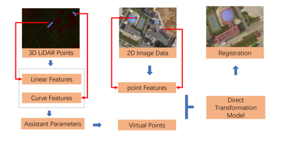
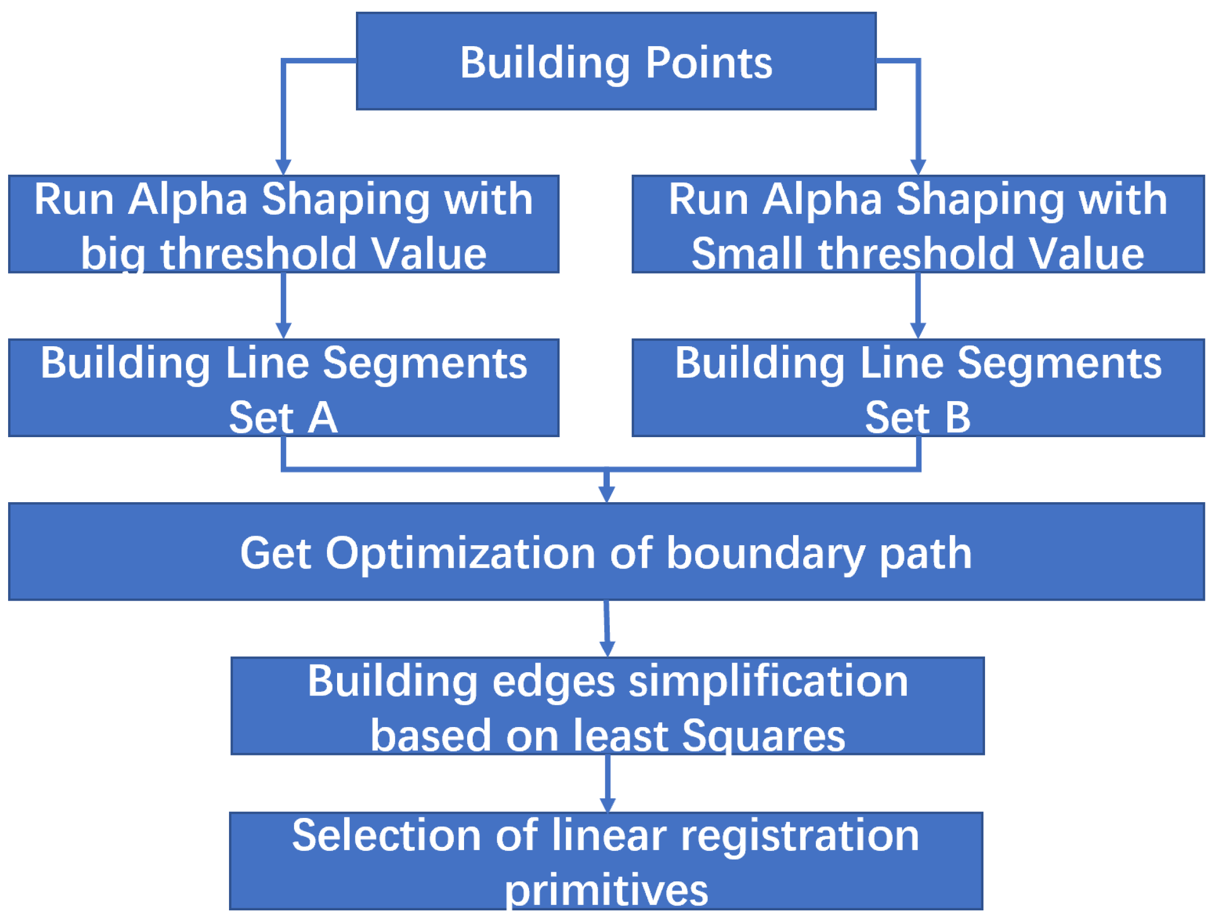
The workflow of the proposed method is shown in Figure 1, and the rest of this paper is organized as follows: After giving a short description for the notations used in this paper, Section 2 describes the technique of how LiDAR data are firstly employed for linear feature detection. As the VPs can be generated from two kinds of linear features and the expression of the VPs from different types of the linear features, all the details will be shown in Section 3. In Section 3, a direction registration transformation model is also used to perform the registration processing and, during the processing, all the primitives with large errors can be excluded automatically. A direct transformation function based on collinearity equations is proposed and four test sites will be used to implement the experiment and discussions in Section 4. Finally, the experimental conclusions will be drawn out in Section 5.
2. Detection and Selection of the Linear Registration Primitives
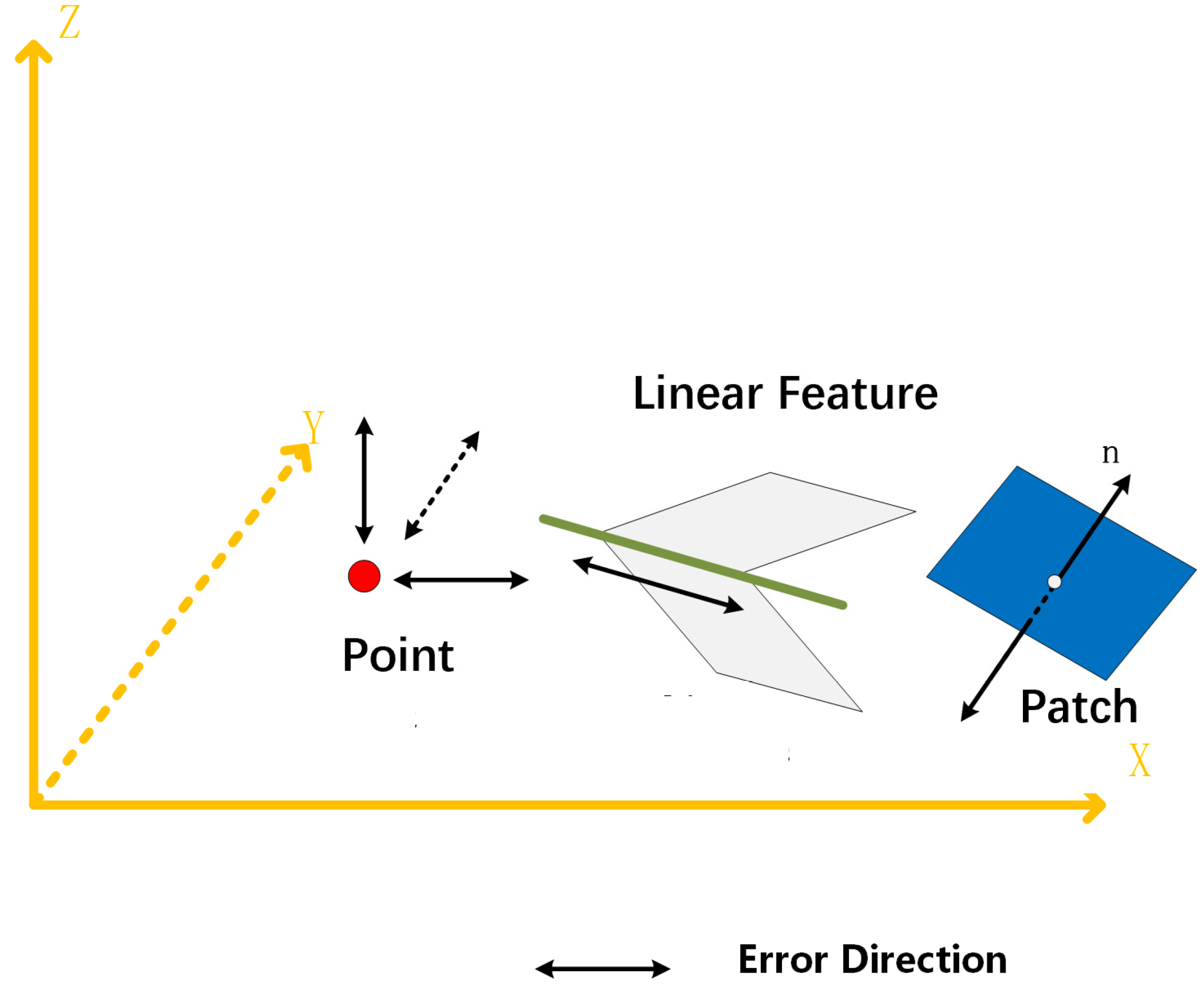
As mentioned in the introduction, registration based on primitives starts from the extraction of salient features, which include point, linear, and planar features, as Figure 2 shows. LiDAR point cloud has semi-discrete random characteristics, so the three types of registration primitives all have specific new features on the LiDAR point cloud, as shown in Table 2. Point registration primitives have random characteristics in LiDAR point cloud and there are error offsets along the three directions of the coordinate axis. The line and patch features in the point cloud are usually generated or fitted by multiple points, so the influence of the discrete error can be greatly reduced [49]. However, the three types of registration primitive have different mathematical expression, and the mathematical expression complexity in Table 2 indicates the difficulty of mathematical expression of each feature. The simpler the expression of registration primitives, the simpler the registration model and the smaller the registration process error.
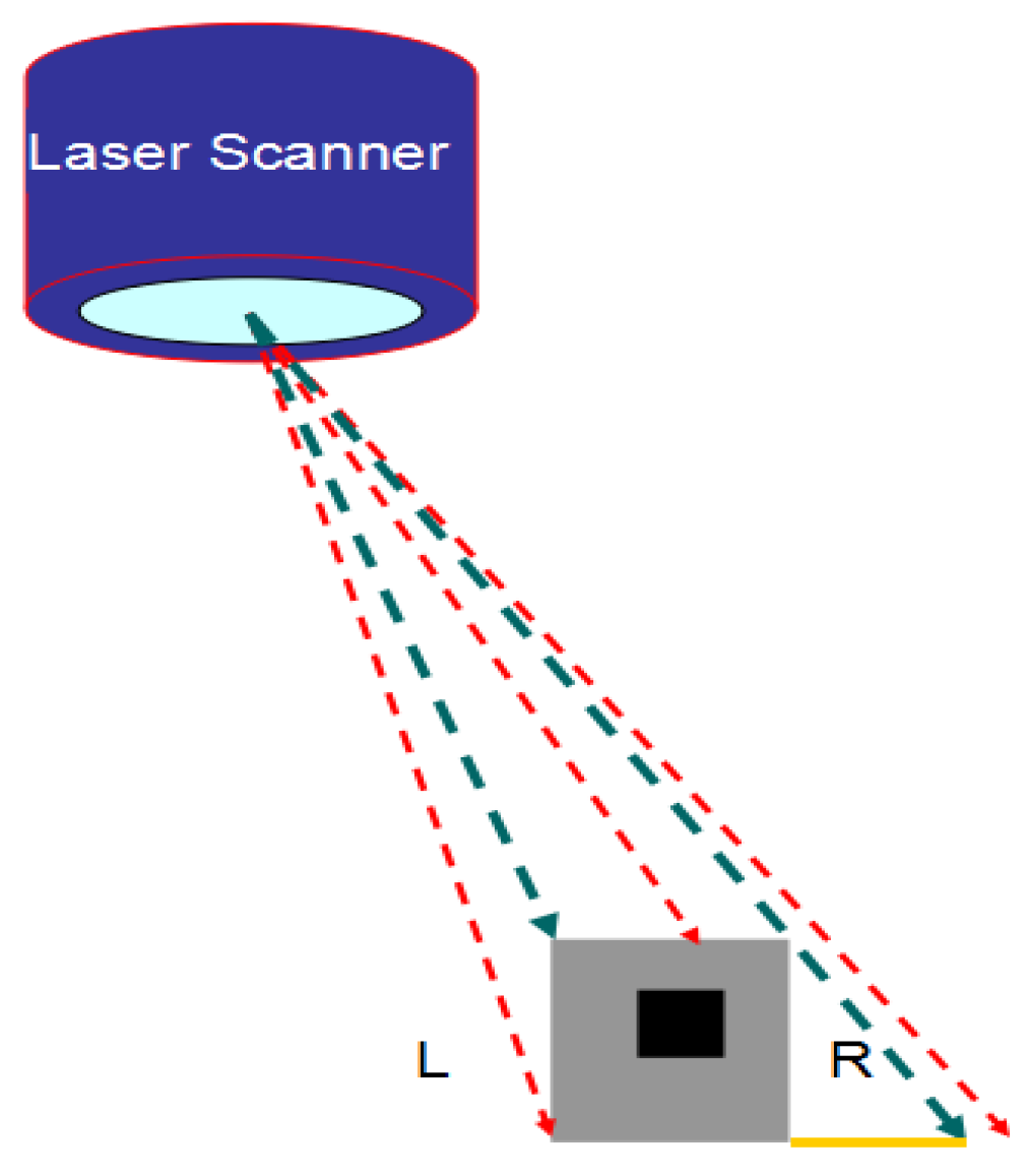
Line features are obtained from the intersection of patches and the accuracy depends on the extraction accuracy of patches. In LiDAR point cloud, there are random errors in directly selected point features and the errors are often greater due to the occlusion of ground objects, as shown in the R region in Figure 3. Therefore, this paper intends to select line or curve features with higher accuracy to represent the point features and realize the high-precision extraction of the registration point primitive. Therefore, the key attributes of this section are the detection and selection of the line and curve features.
2.1. Building Edges Extraction and Feature Selection
Building outlines have distinguishable features that include linear features and curve features, and many methods can be used to extract building outlines from the LiDAR data. To eliminate the semi-random discrete characteristics of point cloud data and obtain high-precision linear registration primitives, the patch intersection can be seen as the most reliable way [50]. In other words, the linear features with wall point cloud should be the first choice for the registration primitives in the L side, as Figure 3 shows. However, the general method of tracking the plane profile of buildings based on airborne LiDAR data is to convert the point cloud into the depth image, then use an image segmentation algorithm to segment the depth image, and finally, use the scanning line method and neighborhood searching method to track the building boundary [51]. The problem of the abovementioned process is that the edge tracked is the rough boundary of the discrete point set, which has low accuracy. Some researchers have also studied the method of extracting the contour directly from the discrete point set. For example, Sampath A et al. [52] proposed an edge tracking algorithm based on plane discrete points. The algorithm takes the edge length ratio as the constraint condition, reduces the influence of the point density, and improves the adaptability for the edge extraction of the slender feature or uneven distribution, but an unsuitable threshold setting can cause the edge excessive contraction. Alpha shapes algorithm was first proposed by Edelsbruuner et al. [53]. Later, many researchers improved upon it and have applied it to the field of airborne LiDAR data processing, because the algorithm has perfect theory and high efficiency and can also deal with complex building contour extraction conditions (e.g., curved building outlines). However, the alpha shapes algorithm is not suitable for uneven data distribution and the selection of algorithm parameters is also difficult. Therefore, to deal with the above problems, this paper proposes a double threshold alpha shapes algorithm to extract the contour of the point set. Then, the initial contour is simplified by using the least square simplification algorithm so that a candidate linear registration primitive satisfying the requirements is generated. Finally, the linear features with wall points can be selected as the registration primitive including straight line features and curve features. Figure 4 illustrates the framework of the proposed linear extraction method.
2.2. Contour Extraction Based on Double Threshold Alpha Shapes Algorithm
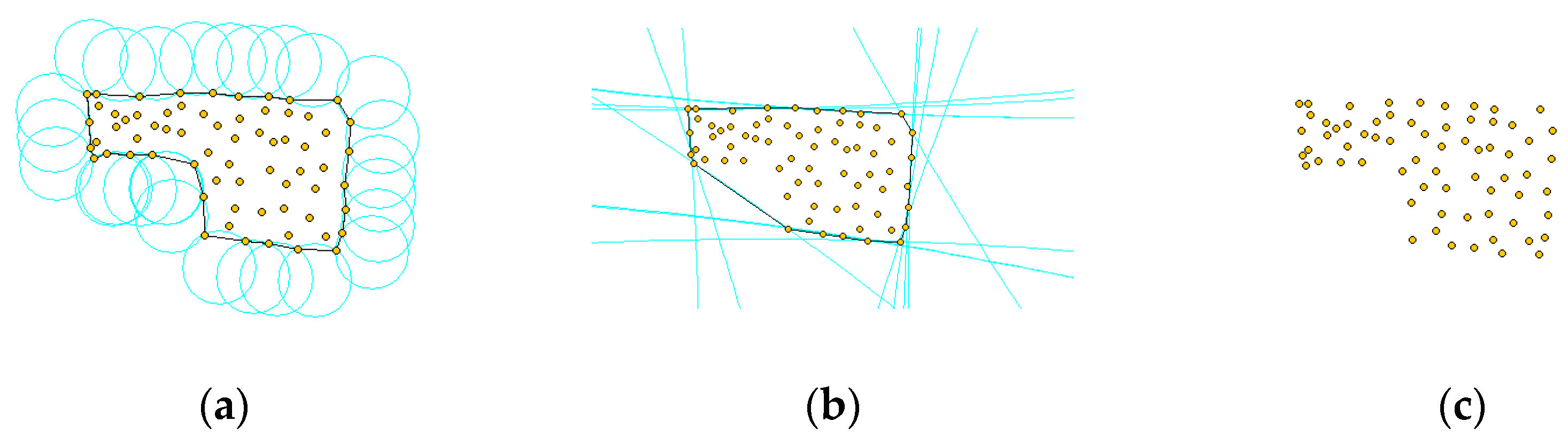
Restoring the original shape of a discrete (2D or 3D) point set is a fundamental and difficult problem. In order to effectively solve the problem, a series of excellent algorithms have been proposed, and the alpha shapes algorithm [54] is one of the best. The alpha shapes algorithm is a deterministic algorithm with a strict mathematical definition. For any finite point set S, the shape of the point set δS obtained by the alpha shapes algorithm is definite. In addition, the user can also control the shape δS of set S by adjusting the unique parameter α of the algorithm. In addition to formal definitions, the alpha shapes algorithm can also use geometric figures for intuitive description. As shown in Figure 5a, the yellow points constitute a point set S; a circle C with a radius of α rolls around the point set S as closely as possible. During the rolling process, the circle C cannot completely contain any point in the point set. Finally, the intersection of the circle C and the point set S is connected in an orderly manner to obtain the point shape set, the shape of which is called the α-shape of the point set S. For any point set S, there are two specific α-shapes: (1) When α approaches infinity, the circle C degenerates into a straight line on the plane, and the point set S is on the same side of the circle C at any given time. Therefore, α-shape is equivalent to the convex hull of the point set S (as shown in Figure 5b); (2) When α approaches 0, since the circle C can roll into the point set, each point in set S is an independent individual, so the shape of the point set is the point itself (as shown in Figure 5c).
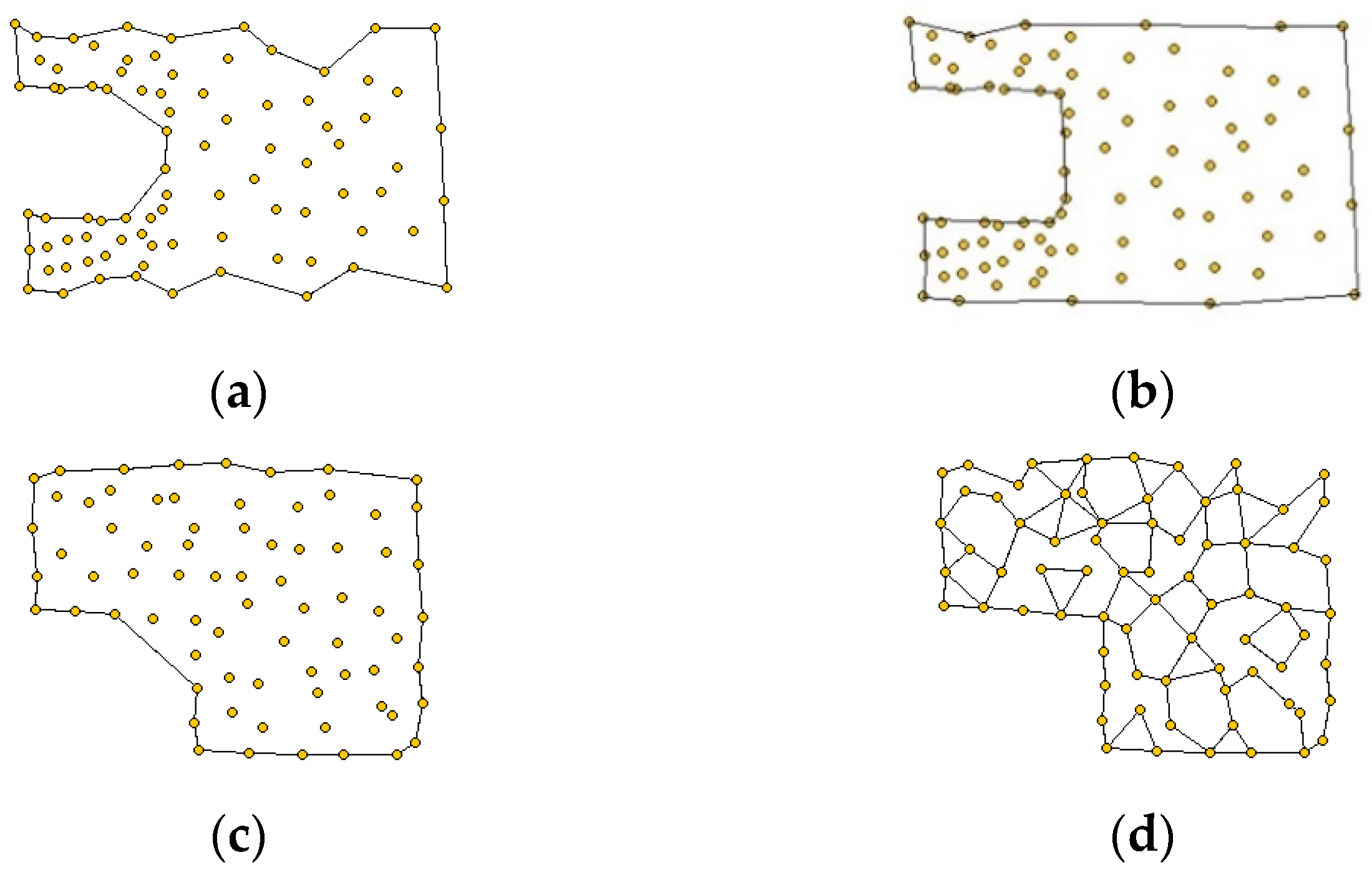
Considering the excellent performance of the alpha shapes algorithm, many researchers have proposed to use the alpha shapes algorithm to directly extract building contours from airborne LiDAR data [54]. However, in practical applications, there are still some problems that need to be solved: (1) Alpha shapes algorithm is mainly suitable for point set data with relatively uniform density, which is determined by the nature of the algorithm, because the fineness of the point set shape is completely determined by the parameters α as shown in Figure 6a,b; the left half of the point set is denser, while the right half is relatively sparse. Figure 6a shows that the alpha shapes algorithm uses a larger α value. The shape shown in Figure 6b is artificially vectorized according to the distribution of the point set and the result is quite different from the shape automatically extracted by the alpha shapes algorithm. It can be seen that a single α value setting of the alpha shapes algorithm cannot adapt to the point set data with varying point densities, and that is exactly the characteristic of the LiDAR point clouds. (2) The alpha shapes algorithm is not very effective when processing concave point sets. If the value of α is large, the concave corners are easily dulled (Figure 6c); if the value of α is small, it is easy to obtain a broken point set shape (Figure 6d). Lach S. R. et al. [55] pointed out that the value of α should be set as one to two times that of the average point spacing and then the shape of the point set obtained at this time is relatively complete and not too broken.
In response to the above problems, this paper proposes a dual threshold alpha shapes algorithm. The main idea of the dual threshold alpha shapes algorithm is: (1) According to the judgment criterion of alpha shapes, set two thresholds α1 and α2 (α1 = 2.5α2), and obtain the qualified line segment (LS) sets and about the point set ; Select one of the optional line segments from edge sets where point and point are the two endpoints of . In an undirected graph composed of the edges of the point set and , differing from the condition of , the points p and q are not always adjacent. However, starting from point p and passing through several nodes, it can always reach point q and generate a path—the path with the smallest length is recorded as . Then, set up a path selection mechanism as follows. (2) Select as the final path from and . The same operation is performed to the edge . All the edges in the iterative processing are used to obtain the path set {, , , …}. Finally, all the paths are connected in turn to obtain the high-precision point set shape. The double threshold alpha shapes algorithm is mainly composed of the following two steps, which are described in detail as follows.
- (1)
- Obtaining dual threshold α-shape
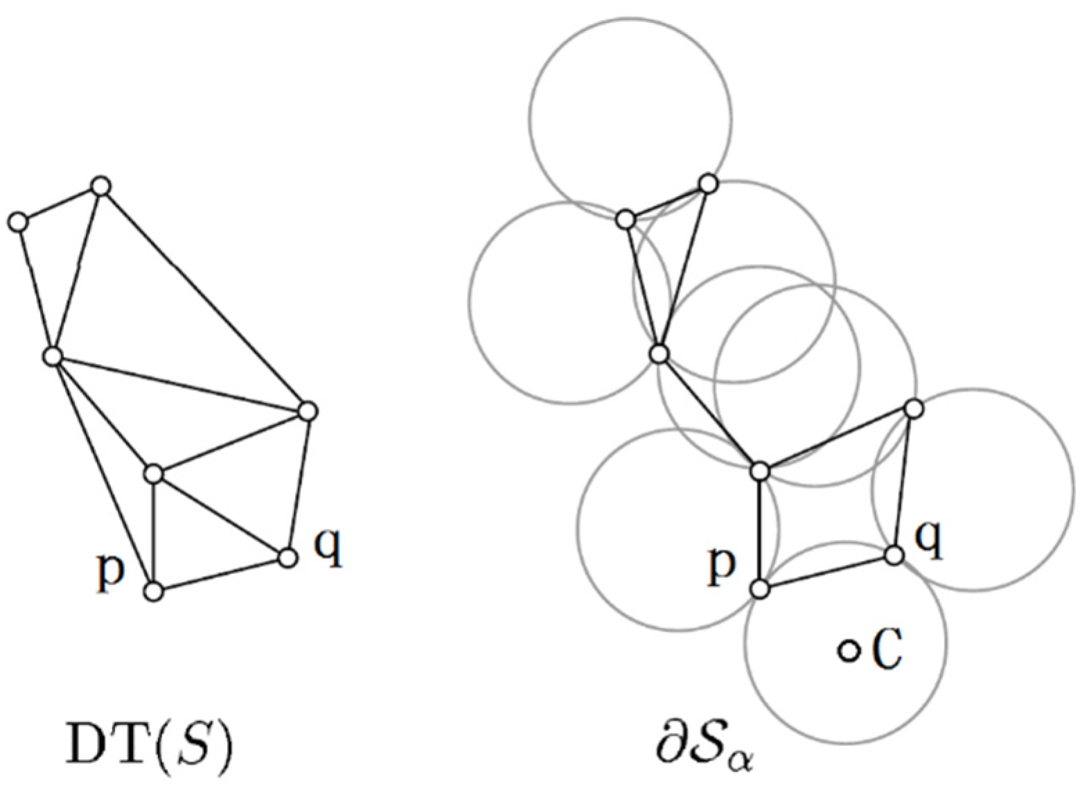
Let be the Delaunay triangulation of the point set S, and and are the α-shapes obtained by the alpha shapes algorithm when the parameters are set to α1 and α2, respectively. Literature has proved that α-shapes under any threshold are all sub-shapes of , which means . Therefore, the process of obtaining α-shape is as follows: firstly, use the point-by-point insertion algorithm to construct the Delaunay triangulation of the point set S (see [52] for the detailed steps of the algorithm) and then perform an alpha shapes algorithm on each edge in in turn, as shown in Figure 7. A line pq (point p and q are adjacent boundary points) is an edge in , circle C is a circle that passes through pq and has a radius of α (the coordinates of the circle center are as shown in (1) and (2), if there is no other vertices in the circle C), then the edge pq belongs to the α-shape.
where:
| Coordinate of point p; | |
| : | Coordinate of point q; |
| Coordinate of point c; c is the center of circle C; | |
| Radius of circle C. |
- (2)
- Optimization of boundary path
In an undirected graph composed of the edges of the point set and . Select any line segment, denoted as the line segment path , with the two endpoints of p and q. Search all paths in the undirected graph with as the starting point and as the end point, calculate the length of each path, and record the path with the smallest length as the boundary path of point and point .
To ensure that the boundary path from point p to point q is the real boundary of the building. In this paper, three criteria are set to determine the path L from the. The judgment criteria are as follows:
- ✧
- As Figure 8a shows, if the length of is more than 5 times that of, then discard and keep ;
- ✧
- As Figure 8b shows, if the two adjacent edges of are close to vertical (more than 60 degree), and all the distances from the endpoints of to any adjacent edge of are small, discard and keep ;
- ✧
- As Figure 8c shows, if the two adjacent sides of and are close to parallel, and the distance from the end point on to is less than a certain threshold (such as half the average point spacing), then is discarded and is retained.
Repeat the above procedure until all the edges of the are complete, then the paths obtained in step (2) are connected in turn to obtain the shape of the point set .
2.3. Straight Linear Feature Simplification Based on Least Square Algorithm
The initial boundary edges of the building obtained by the dual threshold alpha shapes algorithm are very rough and generally need to be simplified first. Douglas Peucker’s [56] algorithm is a classic vector compression algorithm, which is used by many global information systems (GISs). The algorithm uses the vertical distance from the vertex to the line as the simplification basis. If the vertical distance is less than the threshold, the two ends of the line are directly used to replace the current simplification. Otherwise, use the maximum offset point to divide the element into two new elements to be simplified, and then recursively repeat the above operation for the new elements to be simplified, as Figure 9a shows.
This paper proposes a simplification algorithm for linear features based on the least square method, as Figure 9b shows. The algorithm requires two parameters, namely the distance threshold and the length threshold Len. The detailed steps of the algorithm are as follows:
- (1)
- Select three consecutive vertices, A, B, and C, of the polygon in order, use the least square method to fit the straight line L, and calculate the distance from the vertices A, B, C to the straight line L. If any of the distances are greater than , then go to step (4); otherwise, let U = , and go to step (2);
- (2)
- Let set U have two ends p and q, which extend to both directions from p and q, respectively. A new vertex will be added and judged during the growth process. If the distance between the new vertex and the line L is less than, then add it to the set U and use it as a new starting point to continue the growth—otherwise, it will stop growing at the vertex and the direction—until both directions are finished;
- (3)
- Determine the length of the set U. If the length of U is greater than the threshold Len, keep the two ends of the set and discard the middle vertices;
- (4)
- If there are three consecutive vertexes remaining to be judged, go to step (1); otherwise, calculate the size of the length threshold Len. If Len is greater than 2~3 times the average point spacing, reduce the length threshold to Len = 0.8 Len, and go to step (1).
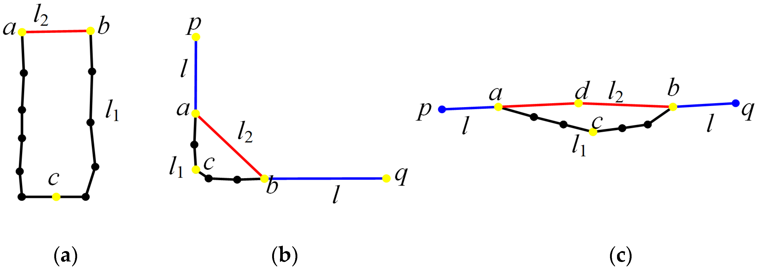
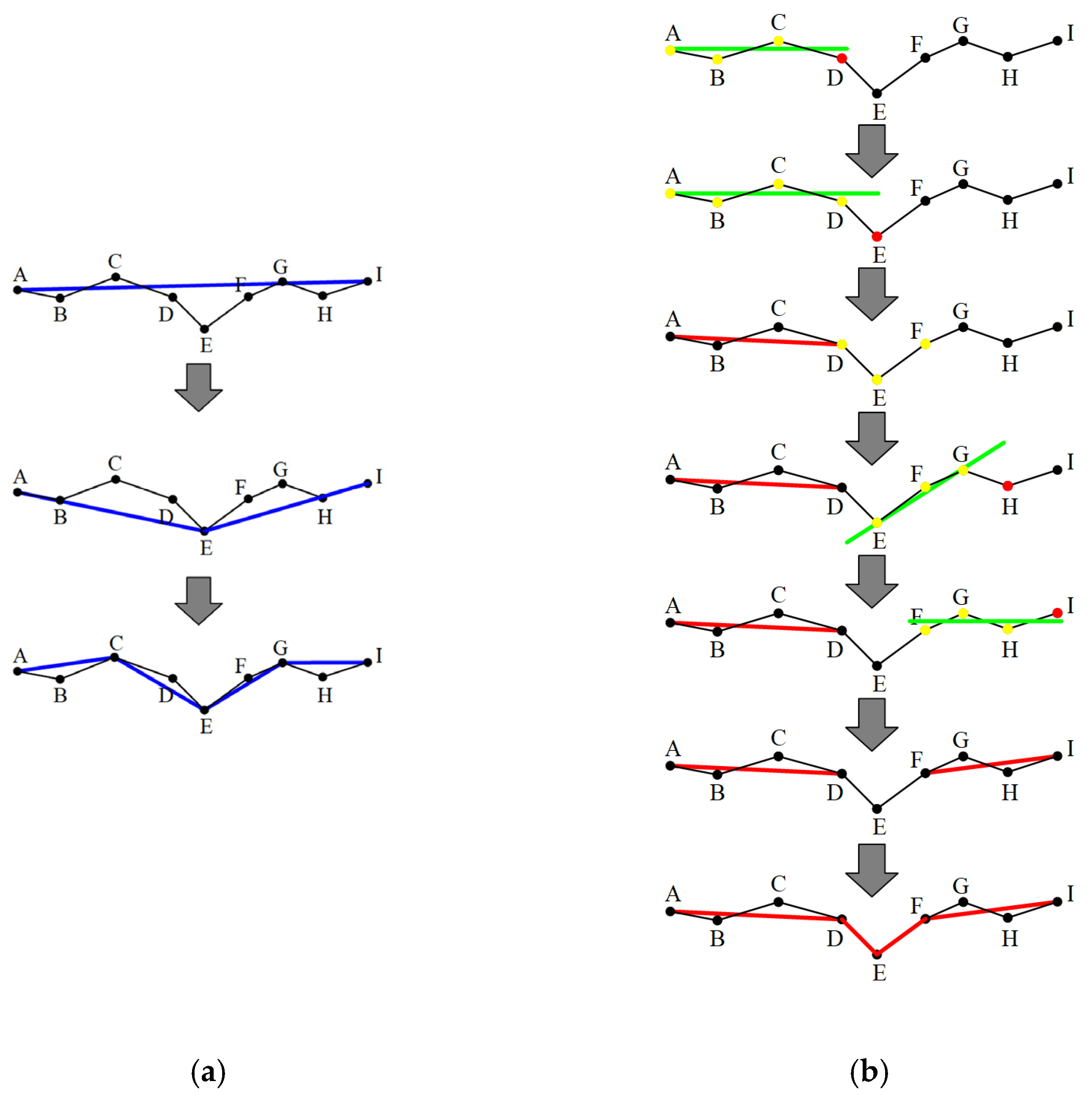
In Figure 9, the black lines are building contours extracted based on double threshold alpha shapes algorithm. Nodes A, B, C, …, I are the boundary key points of the building and the blue line is the intermediate result of the optimization process. In Figure 9a, the blue line is the final result after optimization. In Figure 9b, the red line is a fitting line based on the least square method.
2.4. Curve Feature Simplification Based on Least Square Algorithm
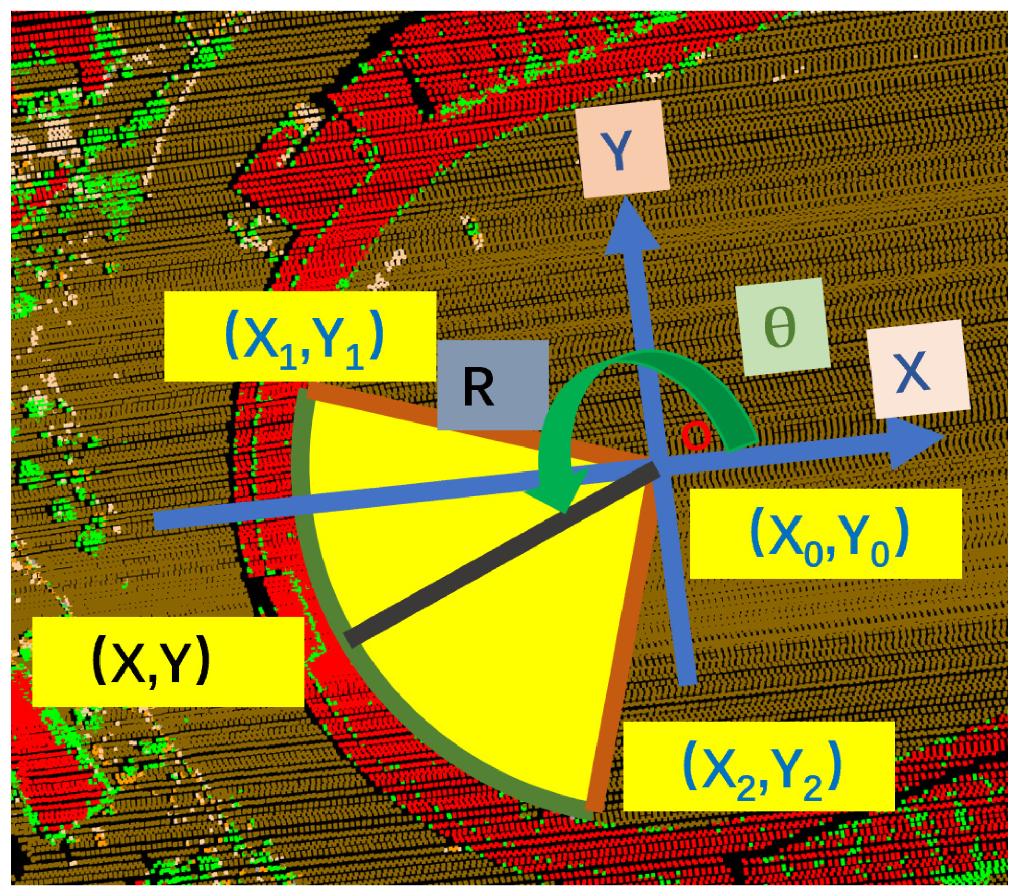
Most of the non-rectangular building boundaries are circular or arc-shaped building outlines, and even an elliptical arc can be regarded as a segmented combination of multiple radius arcs. Therefore, any building boundary curve segment can be regarded as a circular arc segment, defined by rotating a certain radius R around an angle θ, which is shown in Figure 10. In addition, for any arc segment, as long as the number of boundary point clouds on the arc segment N0 > 3 is satisfied, the arc segment C at this time can be fitted by the least square method to obtain the center o, the radius R and the arc segment angle θ (Figure 10). For any arc, the height on the roof boundary is the same, and it can be directly obtained and recorded as Z0 during feature extraction. At this time, any arc can be shown in (3):
Though most commercial and residential buildings have rectangular outlines, arc-shape outlines are not uncommon. In the paper, arc-shape outlines are viewed as arcs of circles. For a given arc, the associated radius and central angle are denoted by R and , respectively, as shown in Figure 10. Denote the coordinates of the circle center by, then any arc can be expressed as follows:
where:
X1, Y1 and X2, Y2: The coordinates of the two distinct end points of the arc;
Z0: The constant height value of the arc which can usually be obtained directly from building edge point.
The three parameters , , and can be calculated using the least square method. At this time, any coordinate on the arc segment can be expressed via (4):
where:
| (X0, Y0, Z0): | The center coordinate of the space circle where the arc is located; |
| R: | The radius of the circle where the arc is located; |
| θ: | The polar coordinate angle of the current point in the transformed coordinate system. |
2.5. The Selection of the Linear Registration Primitives
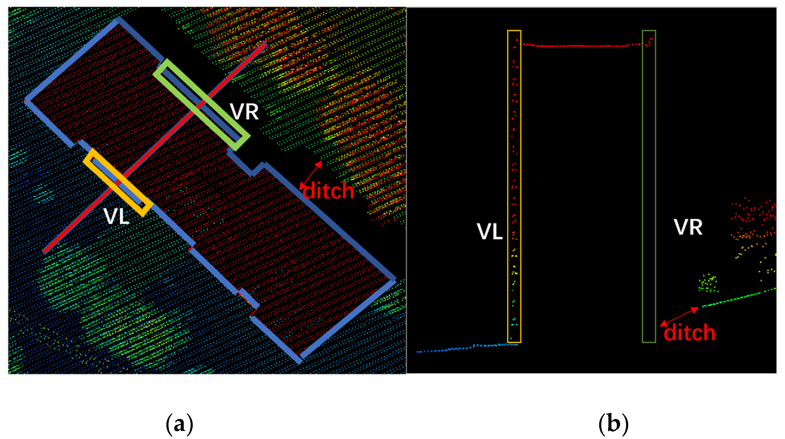
In most cases, a laser beam hits a building at a scanning angle, except when the building is at the nadir of the scanner. This means that some wall facets can be reached by the laser beam, but others cannot, and there is usually a ditch between the wall and the roof edge, as shown in Figure 11. We term wall facets exposed to the laser beam as positives while the others are negatives. That means not all building outlines are accurate enough to meet the registration requirement. To solve the abovementioned problem, only the linear features formed by positive facets are selected as the candidates for registration primitives. By determining that a facet is positive or negative, the following strategy is employed: fitting a given facet by a plane equation so that the normal vector to the plane is obtained, then moving the fitted plane along the normal vector outwardly by a small distance ds, which is determined according to the density of point cloud. A small cuboid is then formed (Figure 11). If the total number of points in the cuboid is larger than a given threshold N, then the line segment formed by projecting the facet onto the ground (xy-plane) is selected as one of the registration primitives.
where:
| The volume of ith cuboid; | |
| : | The ith linear feature segment associated with the ith cuboid; |
| The threshold of the total number of points per unit area; | |
| : | The average height of the linear feature; |
| The distance that the facet moves outwardly along the facet normal vector. |
The abovementioned idea can be shown more intuitively by Figure 11, which gives an outline segment of a building: the vertical view of the building, where VL and VR are the two outline segments formed by projection of the building onto the xy-plane, and its horizontal view from a specific angle. VL is selected as a candidate registration primitive in the paper.
The linear registration primitives extracted by the above method are equivalent to the intersection of the roof surface and the wall surface, so the extraction accuracy is high and the influence of the semi-random attribute of the point cloud is greatly avoided.
3. Registration Primitive Expression and Transformation Model
In this paper, the linear features are selected as the registration primitive. However, compared with point features, linear features require more parameters and complex mathematical models to express, resulting in more complex transformation models being needed. This increases the difficulty of the registration process but decreases the registration accuracy [46]. As pointed out in Section 2, it is far more difficult to extract salient points from LiDAR point cloud than from photogrammetric images. Therefore, we employ point features in image space and linear features in point cloud space, respectively, as the registration primitives (Figure 12).
3.1. The Generation of the VPs
The mathematical expression of line feature or patch feature registration primitives is commonly complex, which often leads to complex registration processes, often introducing processing errors. Therefore, how to reduce or eliminate the random errors caused by the semi-random attribute of the point cloud is the focus task of this section.
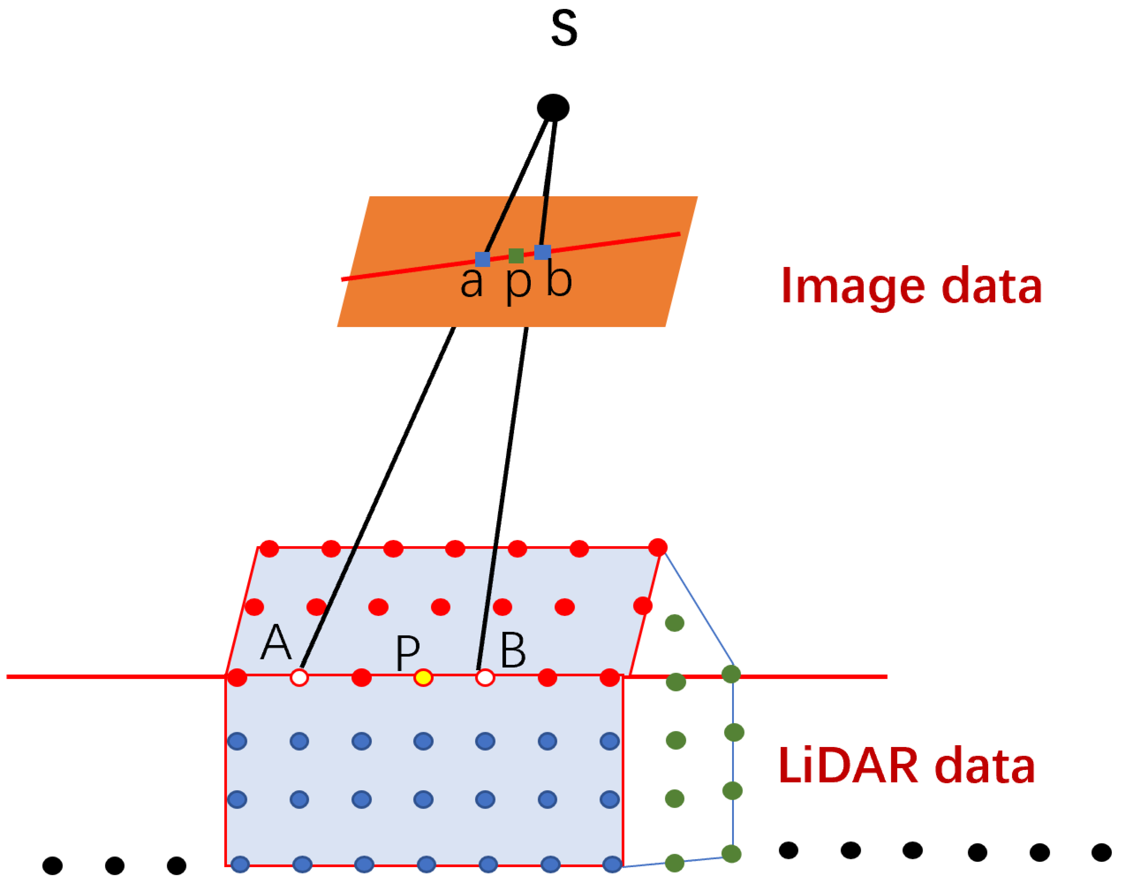
It is obvious that all original registration methodology of the LiDAR 3D points data and the imagery data are point–point, line–line, or point–patch mode, and only the point–point mode can use the direct registration transformation model. However, for the discrete characteristics of the LiDAR points, it is hard to precisely select tie points comparing to the imagery data. As a result, this paper will use the linear features to express the tie point, which can be seen very precisely as the “true value” by introducing an auxiliary parameter, and the expressed “true value” by the linear features can be defined as the virtual point (VP). In this way, precise linear registration primitive and the direct registration model can be utilized simultaneously.
To cater to urban scenes, two kinds of the linear features are counted to generate the respective VPs. Most of the regular primitive features, including the straight lines and regular curves lines, are extracted from the outlines of the buildings in the urban area. In the following sections, we will respectively introduce how to use the two types of linear features to generate the VPs for the registration of image and LiDAR point cloud data.
3.1.1. The VPs from Straight Lines
For high resolution remote sensing images, the horizontal precision is far better than that in LiDAR point cloud, so the VP that is on the straight line—but cannot be selected in the LiDAR point—is used to displace point features to make up the weakness of horizontal information in LiDAR point cloud, as Figure 13 shows. By introducing an auxiliary parameter (λ), and defining the “real” location point, the linear features can be changed into “point” features; this makes the one-step registration transformation model possible.
Any two points express a straight line and any point VP on the line can be expressed by introducing an auxiliary parameter λ. Assuming P is a corresponding point on a roof edge segment LAB of LiDAR space to image point p, introducing a parameter λ, then the coordinates of P in LiDAR space can be expressed by the known PA, PB coordinates and parameter λ, as (7) shows:
where:
| (XA,YA, ZA): | Coordinate of point A in LiDAR data; |
| (XB,YB, ZB): | Coordinate of point B in LiDAR data; |
| (Xvp,Yvp, Zvp): | Coordinate of point VP; |
| λ: | The auxiliary parameter. |
3.1.2. VPs from Curve Features
In addition to straight line features, regular curve features can also be used as registration primitives in LiDAR point cloud space. The boundaries of many buildings have partial arcs or curves, especially in the factory areas, as shown in Figure 14. In the second chapter, the dual threshold alpha shapes algorithm can not only extract straight line features, but also accurately extract precise curve features. Therefore, the building boundary with a certain arc, which is called a regular curve, can be chosen as the registration primitives. Some special and complex buildings, such as the Bird’s Nest of Beijing Olympic Stadium, are not considered.
The regular curve features are expressed in (3), and all the points on the curve features have a constant Z value, which makes it easier to express the VPs as (4) shows. Compared with the straight-line features, the angle θ in the curve feature is introduced as an auxiliary parameter.
where:
| (X0, Y0, Z0): | The center coordinate of the space circle where the arc is located; |
| R: | The radius of the circle where the arc is located; |
| θ: | The polar coordinate angle of the current point in the transformed coordinate system; |
| X1,Y1 and X2,Y2: | The coordinates of the two distinct end points of the arc. |
3.2. The One-Step Transformation Model of the Registration
By introducing an auxiliary parameter, the linear features, including straight line features and curve features, can be seen as virtual points (VPs), and the line–point mode registration can be changed into the point–point mode registration, the registration processing can be converted into the point-to-point pattern. Then the LiDAR point data can be seen as the point cluster of the objects and the registration transformation model is defined in a 2D–3D mode as the formulae (9) and (10) show.
where:
| : | The unknown parameters of the transformation model; |
| t: | The number of the unknown parameters of the transformation model; |
| : | The introduced auxiliary parameter with one pair point–straight line registration primitive; |
| : | The introduced auxiliary parameter with one pair point–curve registration primitive. |
Equation (9) or (10) indicates that each point–line pair of registration primitives can build two equations and introduces one unknown parameter. For the single image, if there are t pair of primitives, the value of the unknown parameters can be resolved. Then for the n-overlap images, one pair of registration primitives can establish 2n equations while introducing only one unknown auxiliary parameter. It follows that all the parameters can be worked out as long as there are enough registration primitives, no matter what kind of transformation models are used. The commonly used geometric correction model can be used as the registration transformation model. For the photogrammetry area, the airborne images and LiDAR data can be integrated using the collinear equations, which would be more reliable with position and orientation system (POS) data. Additionally, the direct linear transformation (DLT) model can be used for both the airborne and ground based datasets. Further, the rational function model (RFM) for the satellite image and the LiDAR point data are also applicative. In this paper, the overall conclusion of the discussion focuses on the airborne LiDAR data and images that have the initial exterior orientation parameters (EOPs).
3.3. The Coefficient Matrix of the VPs
Supposing elements of interior orientation are known and there is no camera error, then we can use first order Tailor expansion for (9) and establish error equation for the straight-line features as (11) shows:
where:
| : | The residual variables; |
| : | The constant value of the linearization equation; |
| : | The coefficients of the transformation model parameters in the linearization equation; |
| : | The coefficients of the auxiliary parameter in the linearization equation; |
| : | The number of the unknown parameter of the transformation model; |
| : | The change value of the auxiliary parameter . |
Making use of Tailor expansion for (11), one point–line registration primitive can build two equations, and for n point–line registration primitives in one image, there will be 2n linearization equations for which we can establish an error equation as shown in (12).
where:
| : | The residual variables for the ith image; |
| : | The constant value of the linearization equation for the ith image; |
| : | The coefficients of the transformation model parameters in the linearization equation for the ith image; |
| : | The coefficients of the auxiliary parameter in the linearization equation for the ith image; |
| : | The number of the unknown parameter of the transformation model; |
| : | The change value of the auxiliary parameter ; |
| : | The count number. |
For one test site, there will be many images. Assuming the number of images is k, there are k series of transformation parameters, and the whole matrix can be simplified as:
where:
| t: | The number of the unknown parameters of the transformation model; |
| : | The primitive number on the ith image; |
| k: | The number of images; |
| V: | The matrix which consists of residual variables. |
| : | The coefficients of the transformation model parameters in the linearization equation of the ith image; |
| : | The coefficients of the auxiliary parameter in the linearization equation of the ith image; |
| : | The count number. |
For replacing linear feature with point feature in the registration between the remote sensing image and LiDAR point cloud, one auxiliary parameter is introduced for every line in LiDAR space; supposing the overlap is n then we can establish 2n equations. Making use of the principle of least square adjustment to solve the elements of exterior orientation of every image and auxiliary parameter , the space point expressed by the line can gradually approach the true value.
For the curve features, the same assumption as with the straight linear features is employed; supposing elements of interior orientation are known and there is no camera error, then we can use first order Tailor expansion for Equation (10) and establish an error equation for the straight-line features as shown by (14):
where:
| : | The coefficients of the auxiliary parameter from the linearization equation; |
| : | The coefficients of the transformation model parameters in the linearization equation; |
| : | The number of the unknown parameters of the transformation model; |
| : | The change value of the auxiliary parameter . |
Making use of Tailor expansion for (14), one point–curve line registration primitive can build two equations, and for n point–curve line registration primitives in one image, there will be 2n linearization equations from which we can establish an error equation formula as seen in (15).
where:
| : | The residual variables for the ith image; |
| : | The constant value of the linearization equation for the ith image; |
| : | The coefficients of the transformation model parameters in the linearization equation for the ith image; |
| : | The coefficients of the auxiliary parameter in the linearization equation for the ith image; |
| : | The number of the unknown parameter of the transformation model; |
| : | The change value of the auxiliary parameter ; |
| : | The count number. |
Assuming there are k images, of course there will be k series of transformation parameters and the whole matrix can be simplified as:
where:
| t: | The number of the unknown parameters of the transformation model; |
| : | The primitive number on the ith image; |
| k: | The number of images; |
| V: | The matrix which consists of residual variables; |
| : | The coefficients of the transformation model parameters in the linearization equation of the ith image; |
| : | The coefficients of the auxiliary parameter in the linearization equation of the ith image. |
As for the way to introduce auxiliary parameters in the conditions if straight and curve features are different, the coefficient matrix of the λ and θ are different. Take the collinear equation registration model as an example; the details can be seen in (17)–(19).
where:
| : | Camera focal length; |
| (): | Image principal point coordinates of exterior orientation parameter; |
| : | Rotation matrix coefficients based on the external angle elements; |
| (, , ): | Coordinate of point A in LiDAR data; |
| (, , ): | Coordinate of point B in LiDAR data; |
| (, , ): | Coordinate of point VP in LiDAR data; |
| : | The auxiliary parameter; |
| : | The radius of the circle where the curve feature is located; |
| Coordinate of point VP in image space. |
3.4. The Iteration of the Registration Procedure
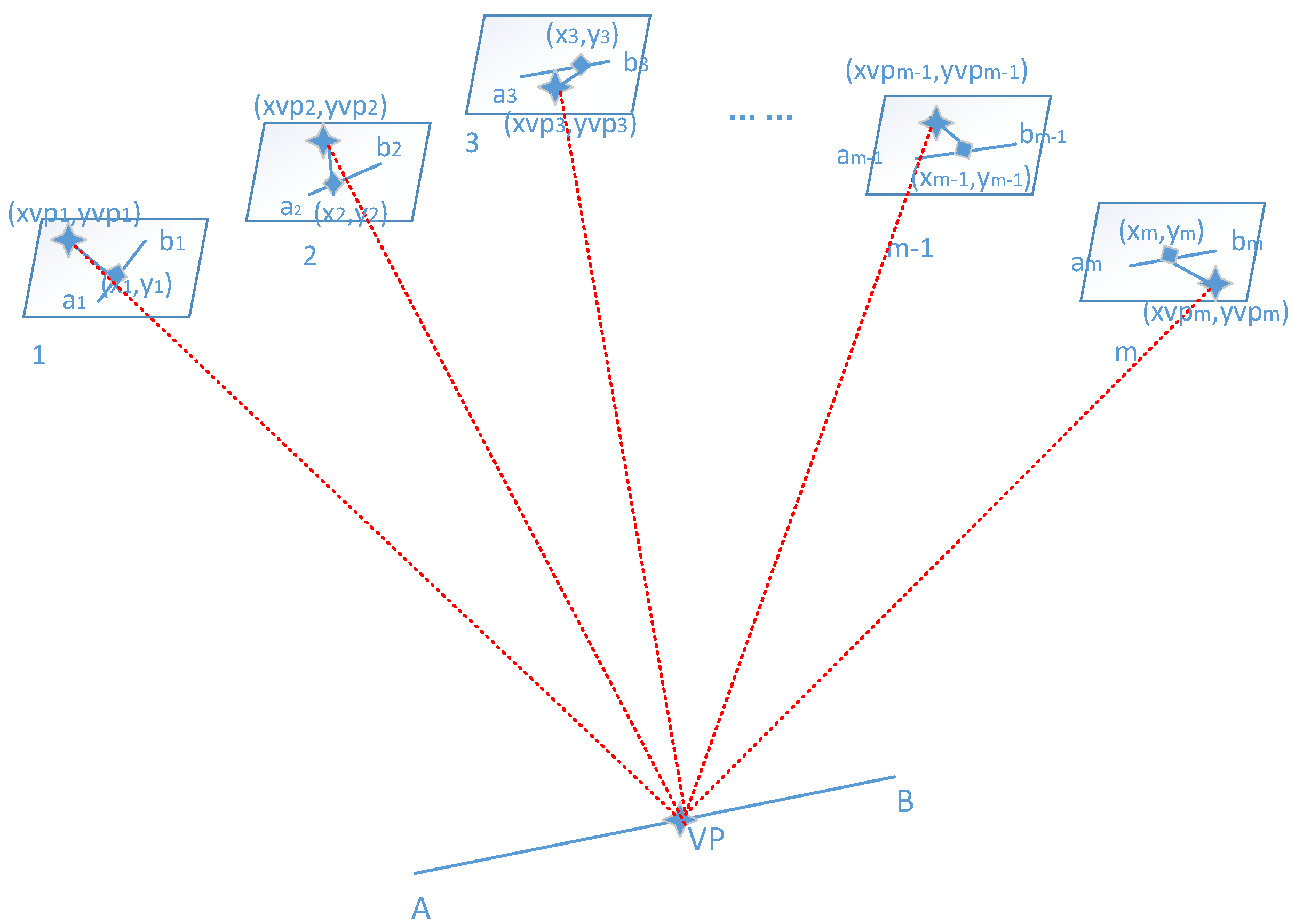
In this paper, we calculate the VP points by the or value and the expression of the straight line and curve features, where the whole process is an iteration procedure such that in each iteration the calculated VPs are approaching the “true” locations. After each iteration, we project the calculated VPs to the images signed as s and the average distance of the s to the corresponding tie points can be used to evaluate the results of the registration, as Figure 15 shows. The number means one linear feature corresponds to m images containing the same feature AB; in other words, the linear feature AB has m overlapping images.
To evaluate when the iteration stops, the is used to measure the transformed VPs as being close enough to the selected control points in the image space as (20) shows.
where:
The average coordinate deviation error of the corresponding points in the image overlap;
The calculated coordinate value of corresponding points in the image by the auxiliary value;
: The coordinate value of corresponding points in the image overlap;
The number of corresponding points in the image overlap.
The methods mentioned in this paper are suitable for both the single image and multi-images mode registration with the LiDAR points data. From Section 3, one pair of point–linear features can build two observation equations and introduce one auxiliary parameter; if there are enough registration features, the unknown parameter of the transformation model and auxiliary parameter can be resolved. For the multi-images, the m overlap image can build 2m observation equations and introduce one auxiliary parameter, so there are more chances of obtaining a redundant observation.
4. Experiments and Results
4.1. Test Data and Results
In this paper, LiDAR and airborne image data for three different sites are used to verify the validity of the algorithm by using it for different regions, as Table 3 shows: an urban region, a rural region, and a mixed region. For different test sites, we used the linear feature and curve feature to test the registration method described in this paper and compared the registration accuracy of the two features.
From Table 3, the four sites cover both urban and rural areas, with different types of cameras and laser scanners, and the registration precision will follow in the next section.
4.2. Registration Accurancy Evaluation Method
To verify the accuracy of the method mentioned in the paper, three test sites are used for the verification. The precise corner points of the buildings are selected as check points. The registration model is used to convert the 3D point coordinates in the LiDAR point cloud into two-dimensional image coordinates (xr, yr), which correspond to the tie point (x, y) on the image, and the horizontal distance deviation between the two coordinates is defined as the registration error. The details of the test sites are shown in Table 4. Among them, the Nanning test site uses straight lines and curves to solve the registration model parameters, and the check points use common check points to achieve registration using straight and curved features, respectively.
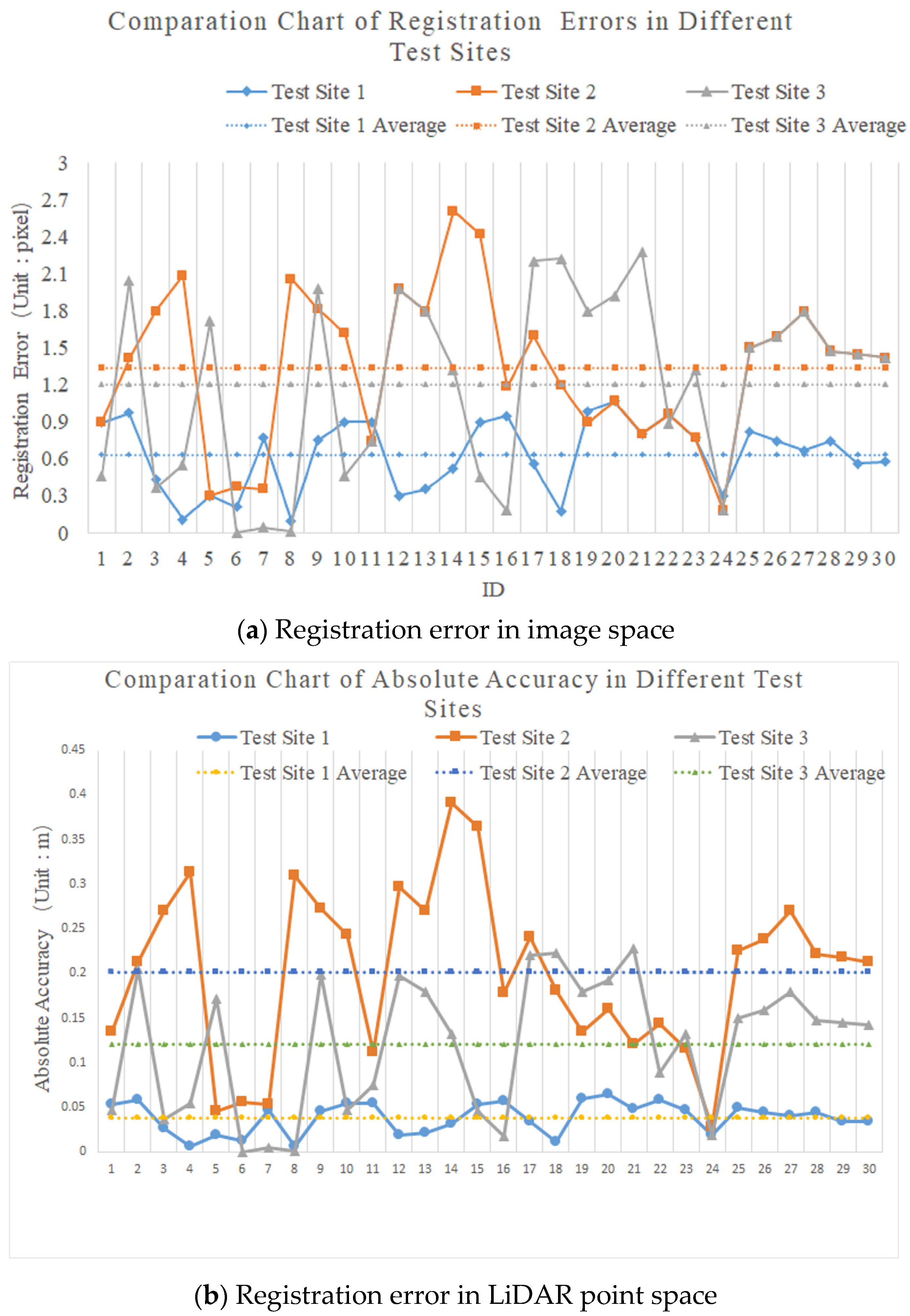
It can be seen from Table 4 that the accuracy of Test Site 1 is 0.636 pixels in image space and 0.0382 m in LiDAR point space. In Test Site 2, the registration accuracy based on the mixed features is 1.339 pixels in image space and 0. 2 m in LiDAR point space. In Test Site 3, using the linear and curved features, respectively, the average accuracy of registration was 1.029 pixels and 1.383 pixels, respectively, in image space, and 0.103 m and 0.138 m, respectively, in LiDAR space. From Test Site 1, the deviation is also low, meaning the registration result is stable. From the above, it is obvious that the registration accuracy is determined by the resolution and the registration primitives. The tests for the registration method were performed on the data of the same test site with straight line feature and curve feature, respectively, and the registration error was almost the same—both within 2 pixels—while the registration accuracy of the straight-line feature was slightly better than that of the curve feature.
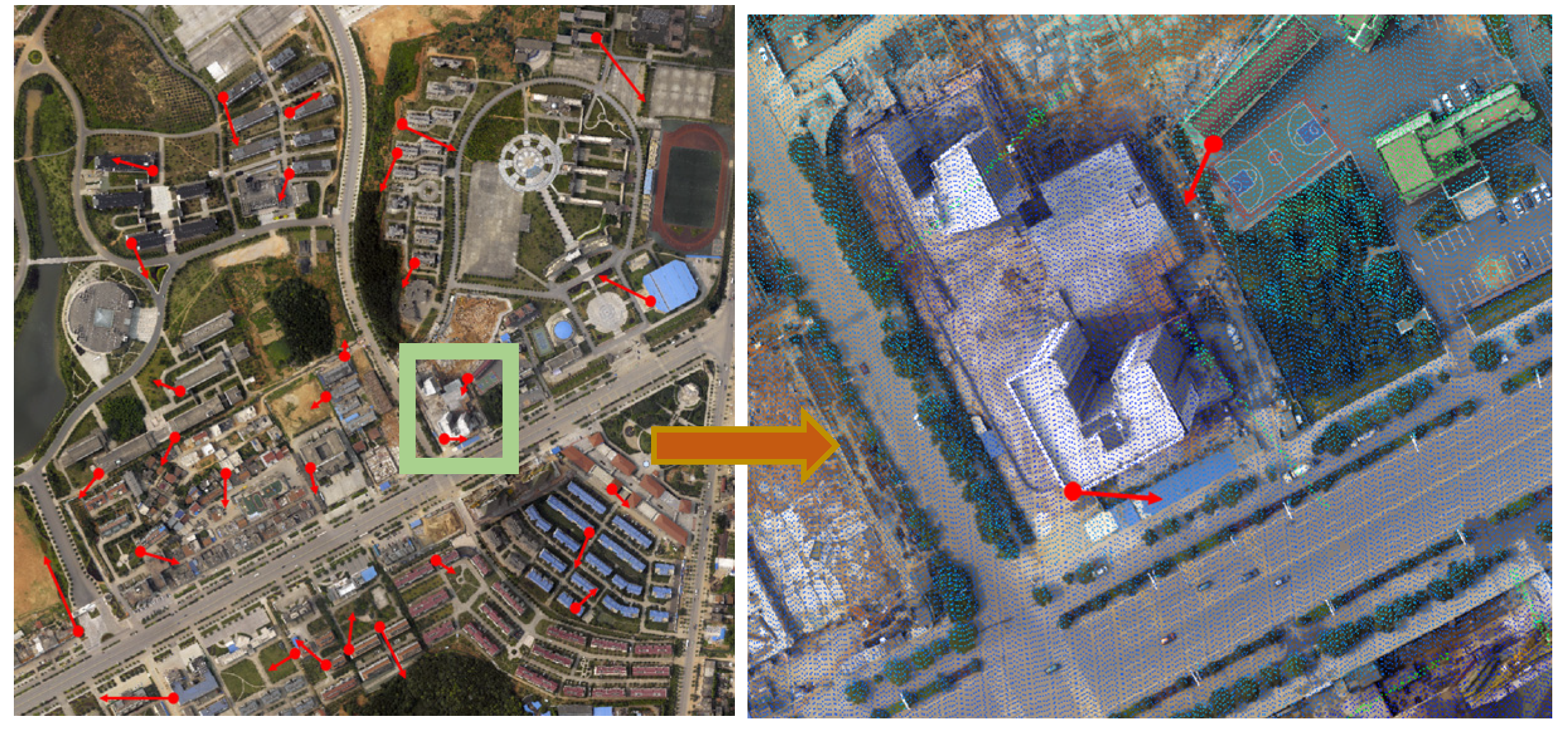
From Table 4 and Figure 16: In test site 1, the registration accuracy of the image obtained by the measuring camera and the LiDAR point cloud data can reach the sub-pixel level of registration accuracy. In test areas 2 and 3, the registration accuracy of the image obtained by the non-measurement camera and the point cloud data is within 3 pixels and the average error is within 2 pixels. As a result, there comes the conclusion that the registration accuracy is also dependent on the camera type. As Figure 17 shows, comparing the error distribution of the checkpoint on the image, the closer to the center of the image, the higher the point registration accuracy will be.
5. The Discussion
As it is well known, the accuracy of the registration depends on many factors such as the choice of the registration primitives, the transformation model, the camera type, and so on. In this paper, all the test data have the original EOPs, then the collinearity equation is used as the registration transformation model.
5.1. The Influence of the Semi-Random Discrete Characteristics
The main advantage of the VPs is to eliminate the effects of semi-random discrete characteristics of the laser point data. The first experiments are designed using the Henan data, in which the images were acquired by the Digital Mapping Camera (DMC), which is minimally impacted by camera lens distortion. To verify the impact of the discrete characteristics of the point cloud data on the registration accuracy, and for the comparison of the registration precision of the point cloud with different point cloud densities, the image is shown in Table 5.
From Table 5, both the average registration accuracy of different density point clouds is less than 1 pixel, even though the point density of dataset 1 is twice that of dataset 2. This shows that the point density has less influence on the registration accuracy. In other words, the method mentioned in the paper greatly reduces the influence of the semi-random discrete characteristics of the point cloud.
5.2. The Influence of the Camera Lens Distortion
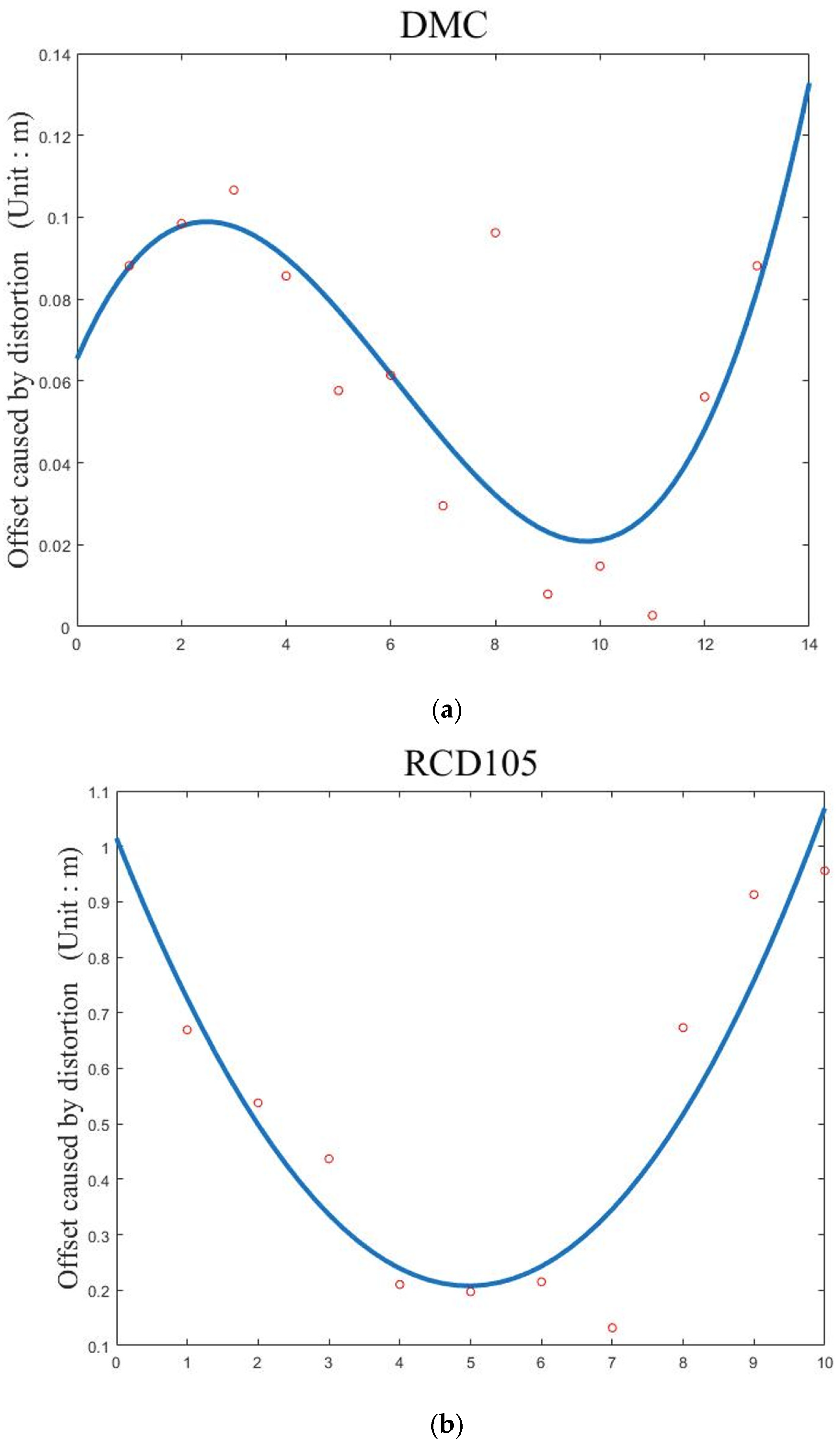
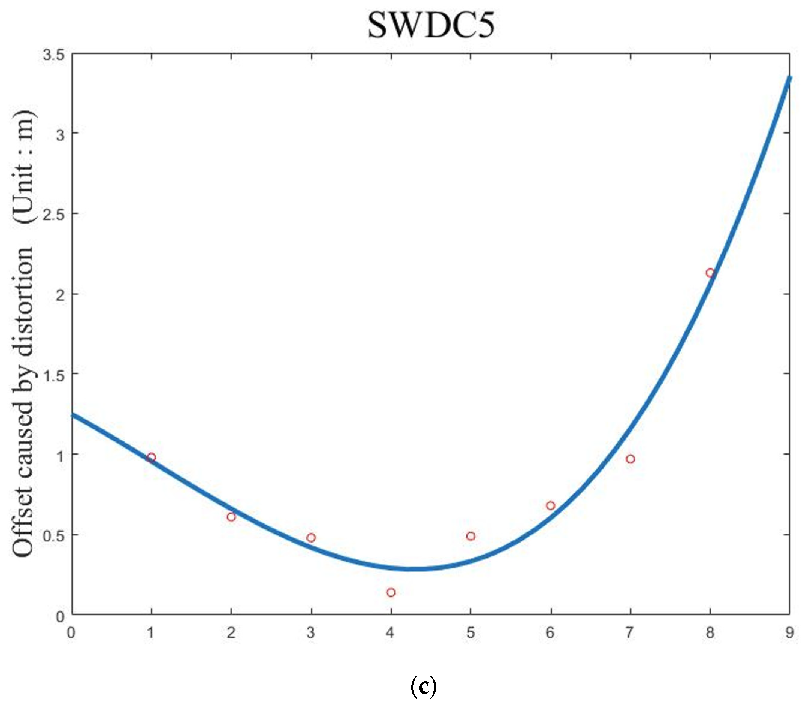
In most cases, the camera equipped on the LiDAR system is not a professional measuring camera and the camera lens distortion usually effects the registration results. In experiment 2, the DMC, RCD105, and SWDC camera are used to test the lens distortion. In order to ignore the effects of the registration primitive and the transformation model in this test, the collinearity equation registration model was used, and the experimental results of 30 check points are shown in Figure 17.
In order to obtain more details of the lens distortion affects, the check points are selected along the center line of the images, and the results are shown in Figure 18.
From Figure 18: For the camera DMC, lens distortion affects along the center line of the images show a fluctuating trend, and that indicates that the influence of the lens distortion is negligible. For the cameras RCD105 and SWDC, the check point that is the farthest away from the center maximizes the error. Assume d is the pixel distance from the image center and the curve of the error along the center line is the cubic function of distance. Then, the registration model collinearity equation used in the experiment can be changed by adding three times polynomial functions in the image space.
where:
and Three times polynomial functions of the and ;
The center points coordinate of the image, but the new rigorous transformation model will add 16 unknown parameters, and as a result, more registration primitives are needed.
5.3. The Effects of Registration Primitive Types
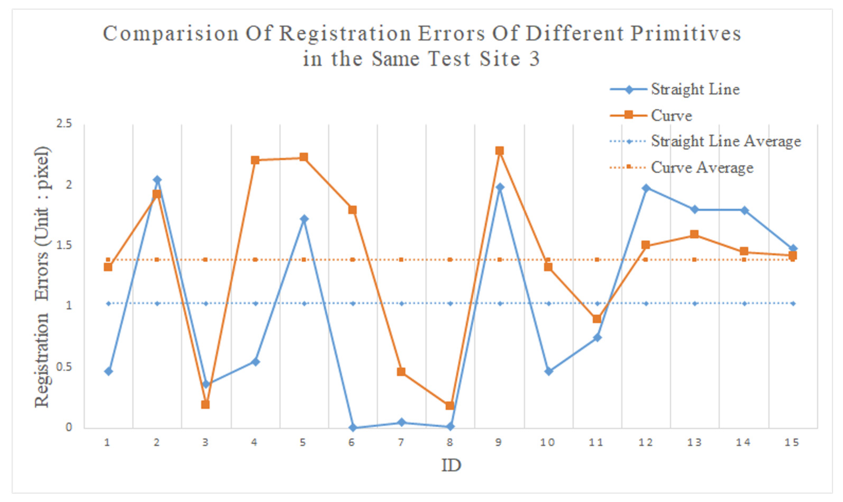
In this paper, the VPs are generated from the straight lines and curves to cater to various conditions of the data that cover different types of terrain. To test the influence of the feature types, the Xianning I and Xinning II test data, which share many common properties but not the registration primitive features, are used. The experimental results are shown in Table 6 and Figure 19.
From Table 6 and Figure 19, the registration error trends of the two features are basically the same. The registration accuracy of the straight-line feature is slightly better than that of the curve feature. The reason is that the virtual point coordinates obtained after the registration based on the straight-line feature are generally the corner point of the building. For curve features, after the iteration, the virtual point coordinates obtained after the registration iteration are generally points on the feature rather than corner points of the building. Therefore, the influence of the semi-random discrete characteristics will be relatively large and that will affect the final configuration.
5.4. The Results Comparation with Other Method
This paper proposes a novel method for registration of the two datasets acquired in urban scenes by using a direct transformation function and VP registration primitives that can be generated from the straight line or curve features as control information. The whole registration processing can avoid the semi-random discrete error and process error. This paper compares the results of similar papers in the previous five years (from year 2016 to year 2021), as Table 7 shows, in which the best results of each paper have been listed. It is obvious that, whether the accuracy of image space or the accuracy of laser point cloud space, the method in this paper has obvious advantages. The other two methods are multi-step registration, and process errors will be introduced in the process of registration. Furthermore, in Bai Zhu’s method, the intensity image sampling from the LiDAR point cloud data is also one of the reasons for the decline of data accuracy, and the registration accuracy will be affected. In addition, in Bisheng Yang’s method, the image and LiDAR point data are collected by the unmanned aerial vehicle, equipped with a poor POS system, and that will lead to poor registration accuracy. The method of this paper is suitable for both the single and multiple images situation to registration with the LiDAR points. However, in Bisheng Yang’s method, it is only suitable for multiple image registration with LIDAR point cloud because of the image sequence matching process. Similarly, because the process of generating point clouds by image sequence dense matching is very time consuming, Yang’s method is the most time-consuming. Followed by Bai Zhu’s method, it is also time consuming to sample laser point clouds into intensity images with a certain resolution. However, the method in this paper does not involve multi process operation steps but direct registration, so the registration process takes the least time.
6. Conclusions
In this article, we propose a new method of LiDAR point cloud and image registration based on virtual points. This method first uses the extracted precise building outlines to generate virtual points. Considering the edges of some buildings are not necessarily regular rectangles, but also curve features, we propose a conversion model with only one auxiliary parameter to achieve registration. This unique parameter makes the registration model simpler and more accurate.
In Section 4, this paper uses four sets of experiments to test the registration of image data and LiDAR point data based on virtual points, and finally verifies the following three conclusions:
- (1)
- Due to the introduction of auxiliary parameters in the line and curve features, the registration method using the direct transformation model can greatly eliminate processing errors and the influence of semi-random attributes of the point cloud data. Without the influence of lens distortion, the registration accuracy can reach the sub-pixel level with respect to the image.
- (2)
- There is lens distortion in the images obtained by non-measuring cameras. The farther away from the image center, the greater the influence of lens distortion. Therefore, to obtain higher registration accuracy, the image with lens distortion must first be eliminated.
- (3)
- Different registration features have little effect on registration accuracy. Experiments show that the registration accuracy of straight-line features is slightly better than that of curve features, mainly because the accuracy of virtual points is affected by semi-discrete properties.
From the above conclusions, to achieve high-precision image and point cloud registration accuracy, the first task is to eliminate the influence of point cloud semi-random discrete characteristics. With the continuous upgrade of LiDAR equipment, the point density is becoming denser, and high-registration accuracy is more possible. In future work, using the original transformation model parameter, we are committed to achieving automatic matching of point clouds and images.
Author Contributions
C.Y. conceived and designed the experiments; C.Y. and H.M. (Hongchao Ma) performed the experiments; C.Y. and H.M. (Haichi Ma) analyzed the data; C.Y. and W.L. wrote the paper. All authors have read and agreed to the published version of the manuscript.
Funding
This research is funded and supported by National Key R&D Program of China (2018YFB0504500), National Natural Science Foundation of China (No. 41101417), and National High Resolution Earth Observations Foundation (11-H37B02-9001-19/22).
Conflicts of Interest
The authors declare there is no conflict of interest regarding the publication of this paper. The founding sponsors had no role in the design of the study; in the collection, analyses, or interpretation of data; in the writing of the manuscript; or in the decision to publish the results.
References
- Zhou, G.Q.; Zhou, X. Seamless Fusion of LiDAR and Aerial Imagery for Building Extraction. IEEE Trans. Geosci. Remote Sens. 2014, 52, 7393–7407. [Google Scholar] [CrossRef]
- Armenakis, C.; Gao, Y.; Sohn, G. Co-registration of aerial photogrammetric and LiDAR point clouds in urban envi-ronments using automatic plane correspondence. Appl. Geomat. 2013, 5, 155–166. [Google Scholar] [CrossRef]
- Koetz, F.B.; Morsdorf, S.; van der Linden, T.; Curt, B. Allgöwer. Multi-source land cover classification for forest fire manage-ment based on imaging spectrometry and LiDAR data. For. Ecol. Manag. 2008, 256, 263–271. [Google Scholar] [CrossRef]
- Awrangjeb, M.; Zhang, C.; Fraser, C.S. Automatic extraction of building roofs using LIDAR data and multispec-tral imagery. ISPRS J. Photogramm. Remote Sens. 2013, 83, 1–18. [Google Scholar] [CrossRef] [Green Version]
- Yang, L.; Sheng, Y.; Wang, B. 3D reconstruction of building facade with fused data of terrestrial LiDAR data and optical image. Optik 2016, 127, 2165–2168. [Google Scholar] [CrossRef]
- Csatho, B.; Schenk, T.; Kyle, P.; Wilson, T.; Krabill, W.B. Airborne laser swath mapping of the summit of Ere-bus volcano, Antarctica: Applications to geological mapping of a volcano. J. Volcanol. Geotherm. Res. 2008, 177, 531–548. [Google Scholar] [CrossRef]
- Skaloud, J.; Lichti, D. Rigorous approach to bore-sight self-calibration in airborne laser scanning. ISPRS J. Photogramm. Remote Sens. 2006, 61, 47–59. [Google Scholar] [CrossRef]
- Palenichka, R.M.; Zaremba, M.B. Automatic Extraction of Control Points for the Registration of Optical Satellite and LiDAR Images. IEEE Trans. Geosci. Remote Sens. 2010, 48, 2864–2879. [Google Scholar] [CrossRef]
- Xiong, B.; Elberink, S.O.; Vosselman, G. A graph edit dictionary for correcting errors in roof topology graphs reconstructed from point clouds. ISPRS J. Photogramm. Remote Sens. 2014, 93, 227–242. [Google Scholar] [CrossRef]
- Wu, Z.; Ni, M.; Hu, Z.; Wang, J.; Li, Q.; Wu, G. Mapping invasive plant with UAV-derived 3D mesh model in mountain area—A case study in Shenzhen Coast, China. Int. J. Appl. Earth Obs. Geoinform. 2019, 77, 129–139. [Google Scholar] [CrossRef]
- Lopatin, J.; Fassnacht, F.E.; Kattenborn, T.; Schmidtlein, S. Mapping plant species in mixed grassland communities using close range imaging spectroscopy. Remote Sens. Environ. 2017, 201, 12–23. [Google Scholar] [CrossRef]
- Lu, B.; He, Y. Species classification using Unmanned Aerial Vehicle (UAV)-acquired high spatial resolution imagery in a heterogeneous grassland. ISPRS J. Photogramm. Remote Sens. 2017, 128, 73–85. [Google Scholar] [CrossRef]
- Johnson, K.M.; Ouimet, W.B.; Dow, S.; Haverfield, C. Ouimet, Samantha Dow and Cheyenne Haverfield. Estimating Historically Cleared and Forested Land in Massachusetts, USA, Using Airborne LiDAR and Archival Records. Remote Sens. 2021, 13, 4318. [Google Scholar] [CrossRef]
- Kwan, C.; Gribben, D.; Ayhan, B.; Bernabe, S.; Plaza, A.; Selva, M. Improving Land Cover Classification Using Extended Multi-Attribute Profiles (EMAP) Enhanced Color, Near Infrared, and LiDAR Data. Remote Sens. 2020, 12, 1392. [Google Scholar] [CrossRef]
- Bodensteiner, C.; Huebner, W.; Juengling, K.; Mueller, J.; Arens, M. Local multi-modal image matching based on self-similarity. In Proceedings of the 2010 IEEE International Conference on Image Processing, Hong Kong, China, 26–29 September 2010; pp. 937–940. [Google Scholar] [CrossRef]
- Bodensteiner, C.; Hubner, W.; Jungling, K.; Solbrig, P.; Arens, M. Monocular camera trajectory optimization using Li-DAR data. In Proceedings of the IEEE International Conference on Computer Vision Workshops (ICCV Workshops), Barlcelona, Spain, 6–13 November 2011; pp. 2018–2025. [Google Scholar]
- Al-Manasir, K.; Fraser, C.S. Automatic registration of terrestrial laser scanner data via imagery. Photogramm. Rec. 2006, 21, 255–268. [Google Scholar] [CrossRef]
- Parmehr, E.G.; Fraser, C.S.; Zhang, C.; Leach, J. Automatic registration of optical imagery with 3D LiDAR data using statistical similarity. ISPRS J. Photogramm. Remote Sens. 2014, 88, 28–40. [Google Scholar] [CrossRef]
- Baltsavias, E.P. Airborne laser scanning: Existing systems and firms and other resources. ISPRS J. Photogramm. Remote Sens. 1999, 54, 164–198. [Google Scholar] [CrossRef]
- Csanyi, N.; Toth, C.K. Improvement of Lidar Data Accuracy Using Lidar-Specific Ground Targets. Photogramm. Eng. Remote Sens. 2007, 73, 385–396. [Google Scholar] [CrossRef] [Green Version]
- Jung, I.-K.; Lacroix, S. A robust interest points matching algorithm. In Proceedings of the Eighth IEEE International Conference on Computer Vision, Vancouver, BC, Canada, 7–14 July 2001; Volume 2, pp. 538–543. [Google Scholar]
- Schenk, T.; Csathó, B. Fusion of LIDAR Data and Aeria1 Imagery for a Complete Surface Description. Int. Arch. Photogramm. Remote Sens. 2002, 34, 310–317. [Google Scholar]
- Baltsavias, E.P. A comparison between photogrammetry and laser scanning. ISPRS J. Photogramm. Remote Sens. 1999, 54, 83–94. [Google Scholar] [CrossRef]
- Habib, A.F. Aerial triangulation using point and linear features. ISPRS J. Photogramm. Remote Sens. 1999, 32, 137–141. [Google Scholar]
- Habib, A.; Lee, Y.; Morgan, M. Bundle Adjustment with Self-Calibration of Line Cameras Using Straight Lines. In Proceedings of the Joint Workshop of ISPRS WG I/2, I/5 and IV/7, Hanover, Germany, 19–21 September 2001. [Google Scholar]
- Habib, A.; Asmamaw, A. Linear Features in Photogrammetry; Departmental Report # 451; The Ohio State University: Columbus, OH, USA, 1999. [Google Scholar]
- Habib, A.F.; Ghanma, M.S.; Morgan, M.F.; Mitishita, E. Integration of laser and photogrammetric data for calibration purposes. Int. Arch. Photogramm. Remote Sens. Spat. Inf. Sci. 2004, 35, 170. [Google Scholar]
- Habib, A.; Ghanma, M.; Mitishita, E. Photogrammetric Georeferencing Using LIDAR Linear and Aeria1 Features. Korean J. Geom. 2005, 5, 7–19. [Google Scholar]
- Yang, B.; Chen, C. Automatic registration of UAV-borne sequent images and LiDAR data. ISPRS J. Photogramm. Remote Sens. 2015, 101, 262–274. [Google Scholar] [CrossRef]
- Lv, F.; Ren, K. Automatic registration of airborne LiDAR point cloud data and optical imagery depth map based on line and points features. Infrared. Phys. Technol. 2015, 71, 457–463. [Google Scholar] [CrossRef]
- Abayowa, B.O.; Yilmaz, A.; Hardie, R.C. Automatic registration of optical aerial imagery to a LiDAR point cloud for generation of city models. ISPRS J. Photogramm. Remote Sens. 2015, 106, 68–81. [Google Scholar] [CrossRef]
- Habib, A.; Schenk, T. A new approach for matching surfaces from laser scanners and optical scanners. Int. Arch. Photogramm. Remote Sens. 1999, 32, 55–61. [Google Scholar]
- Mastin, A.; Kepner, J.; Fisher, J. Automatic Registration of LiDAR and optial images of urban scene. In Proceedings of the IEEE Conference on Computer Vision and Patten Recognition, Miami, FL, USA, 20–25 June 2009; pp. 2639–2646. [Google Scholar]
- Parmehr, E.G.; Fraser, C.S.; Zhang, C.; Leach, J. Automatic Registration of Aerial Images with 3D LiDAR Data Using a Hy-brid Intensity-Based Method. In Proceedings of the International Conference on Digital Image Computing Techniques & Applications, Fremantle, Australia, 3–5 December 2012. [Google Scholar]
- Axelsson, P. Processing of laser scanner data—algorithms and applications. ISPRS J. Photogramm. Remote Sens. 1999, 54, 138–147. [Google Scholar] [CrossRef]
- Zhu, B.; Ye, Y.; Zhou, L.; Li, Z.; Yin, G. Robust registration of aerial images and LiDAR data using spatial constraints and Gabor structural features. ISPRS J. Photogramm. Remote Sens. 2021, 181, 129–147. [Google Scholar] [CrossRef]
- Liu, Y. Improving ICP with easy implementation for free-form surface matching. Pattern Recognit. 2004, 37, 211–226. [Google Scholar] [CrossRef] [Green Version]
- Lowe, D.G. Distinctive Image Features from Scale-Invariant Keypoints. Int. J. Comput. Vis. 2004, 60, 91–110. [Google Scholar] [CrossRef]
- Schutz, C.; Jost, T.; Hugli, H. Multi-feature matching algorithm for free-form 3D surface registration. In Proceedings of the Fourteenth International Conference on Pattern Recognition, Brisbane, QLD, Australia, 20–20 August 1998; pp. 982–984. [Google Scholar]
- Habib, A.; Lee, Y.; Morgan, M. LIDAR data for photogrammetric georeferencing. In Proceedings of the Joint Workshop of ISPRS WG I/2, I/5 and IV/7, Hanover, Germany, 19–21 September 2001. [Google Scholar]
- Wong, A.; Orchard, J. Efficient FFT-Accelerated Approach to Invariant Optical–LIDAR Registration. Geosci. Remote Sens. 2008, 46, 17–25. [Google Scholar] [CrossRef]
- Harrison, J.W.; Iles, P.J.W.; Ferrie, F.P.; Hefford, S.; Kusevic, K.; Samson, C.; Mrstik, P. Tessellation of Ground-Based LIDAR Data for ICP Registration. In Proceedings of the Canadian Conference on Computer and Robot Vision, Windsor, ON, Canada, 28–30 May 2008; pp. 345–351. [Google Scholar]
- Teo, T.-A.; Huang, S.-H. Automatic Co-Registration of Optical Satellite Images and Airborne Lidar Data Using Relative and Absolute Orientations. IEEE J. Sel. Top. Appl. Earth Obs. Remote Sens. 2013, 6, 2229–2237. [Google Scholar] [CrossRef]
- Liu, X. Airborne LiDAR for DEM generation: Some critical issues. Prog. Phys. Geogr. 2008, 32, 31–49. [Google Scholar]
- Habib, A.; Schenk, T. Utilization of ground control points for image orientation without point identification in image space. In Proceedings of the SPRS Commission III Symposium: Spatial Information from Digital Photogrammetry and Computer Vision, Munich, Germany, 5–9 September 1994; Volume 32, pp. 206–211. [Google Scholar] [CrossRef]
- Schenk, T. Determining Transformation Parameters between Surfaces without Identical Points; Technical Report; Photogrammetry No. 15; Department of Civil and Environmental Engineering and Geodetic Science, OSU: Columbus, OH, USA, 1999; p. 22. [Google Scholar]
- Li, J.; Yang, B.; Chen, C.; Habib, A. NRLI-UAV: Non-rigid registration of sequential raw laser scans and images for low-cost UAV LiDAR point cloud quality improvement. ISPRS J. Photogramm. Remote Sens. 2019, 158, 123–145. [Google Scholar] [CrossRef]
- Kilian, J.; Haala, N.; Englich, M. Capture and evaluation of airborne laser scanner data. Int. Arch. Photogramm. Remote Sens. 1996, 31, 383–388. [Google Scholar]
- Habib, A.; Ghanma, M.; Morgan, M.; Al-Ruzouq, R. Photogrammetric and Lidar Data Registration Using Linear Features. Photogramm. Eng. Remote Sens. 2005, 71, 699–707. [Google Scholar] [CrossRef]
- Lee, J.B.; Yu, K.Y. Coregistration of aerial photos, ALS data and digital maps using linear features. KOGSIS J. 2006, 14, 37–44. [Google Scholar]
- Ma, R. DEM generation and building detection from lidar data. Photogramm. Eng. Remote Sens. 2005, 71, 847–854. [Google Scholar] [CrossRef]
- Sampath, A.; Shan, J. Building boundary tracing and regularization from airborne lidar point clouds. Photogramm. Eng. Remote Sens. 2007, 73, 805–812. [Google Scholar] [CrossRef] [Green Version]
- Edelsbrunner, H.; Kirkpatrick, D.; Seidel, R. On the shape of a set of points in the plane. IEEE Trans. Inf. Theory 1983, 29, 551–559. [Google Scholar] [CrossRef] [Green Version]
- De Berg, M.; Van Kreveld, M.; Overmars, M.; Schwarzkopf, O.C. Computational Geometry; Springer: Berlin/Heidelberg, Germany, 2000. [Google Scholar]
- Lach, S.R.; Kerekes, J.P. Robust extraction of exterior building boundaries from topographic LiDAR data. In Proceedings of the Geoscience and Remote Sensing Symposium, Boston, MA, USA, 7–11 July 2008. [Google Scholar]
- Dorninger, P.; Pfeifer, N. A comprehensive automated 3D approach for building extraction, reconstruction, and regulariza-tion from airborne laser scanning point clouds. Sensors 2008, 8, 7323–7343. [Google Scholar] [CrossRef] [PubMed] [Green Version]
Figure 1.
(a) The workflow of the proposed method. Linear and curve features detection, virtual point generation, and registration transformation model. (b) The virtual points feature and point feature in LiDAR point data and images, respectively, and the overlap result of the two data.
Figure 1.
(a) The workflow of the proposed method. Linear and curve features detection, virtual point generation, and registration transformation model. (b) The virtual points feature and point feature in LiDAR point data and images, respectively, and the overlap result of the two data.

Figure 2.
The directions in which error occurs with different feature types.

Figure 3.
The linear features on the L side should be selected as the registration primitive.

Figure 4.
Framework for linear feature detection.

Figure 5.
Alpha shapes algorithm geometry description and two special cases. (a) appropriate α value. (b) α value tends to infinity. (c) α value tends to zero.
Figure 5.
Alpha shapes algorithm geometry description and two special cases. (a) appropriate α value. (b) α value tends to infinity. (c) α value tends to zero.

Figure 6.
Problems with the alpha shapes algorithm. (a) α-shape of uneven point set. (b) Artificial vectorized shape of uneven point set. (c) Excessive α value leads to obtuse angle. (d) small α value leads to fragmentation.
Figure 6.
Problems with the alpha shapes algorithm. (a) α-shape of uneven point set. (b) Artificial vectorized shape of uneven point set. (c) Excessive α value leads to obtuse angle. (d) small α value leads to fragmentation.

Figure 7.
Schematic diagram of boundary extraction based on alpha shapes algorithm.

Figure 8.
Corresponding path filtering of different situation. (a) . (b) the angle between and . (c) and are near the same line .
Figure 8.
Corresponding path filtering of different situation. (a) . (b) the angle between and . (c) and are near the same line .

Figure 9.
Example of processing noisy polygonal line segments. (a) Douglas Peucker’s algorithm processing. (b) The least square method processing.
Figure 9.
Example of processing noisy polygonal line segments. (a) Douglas Peucker’s algorithm processing. (b) The least square method processing.

Figure 10.
In the schematic diagram of coordinate transformation, any point on the arc can be presented by (X0, Y0, Z0), R and θ.
Figure 10.
In the schematic diagram of coordinate transformation, any point on the arc can be presented by (X0, Y0, Z0), R and θ.

Figure 11.
The L side features have dense points because of the wall. (a)The top view of the building walls. (b) The profile of the building walls.
Figure 11.
The L side features have dense points because of the wall. (a)The top view of the building walls. (b) The profile of the building walls.

Figure 12.
The point ‘a’ on the image corresponds to the point A as the tie point. A cannot manually be selected on the laser point cloud. The point A is on the line L and L can be detected in the LiDAR data.
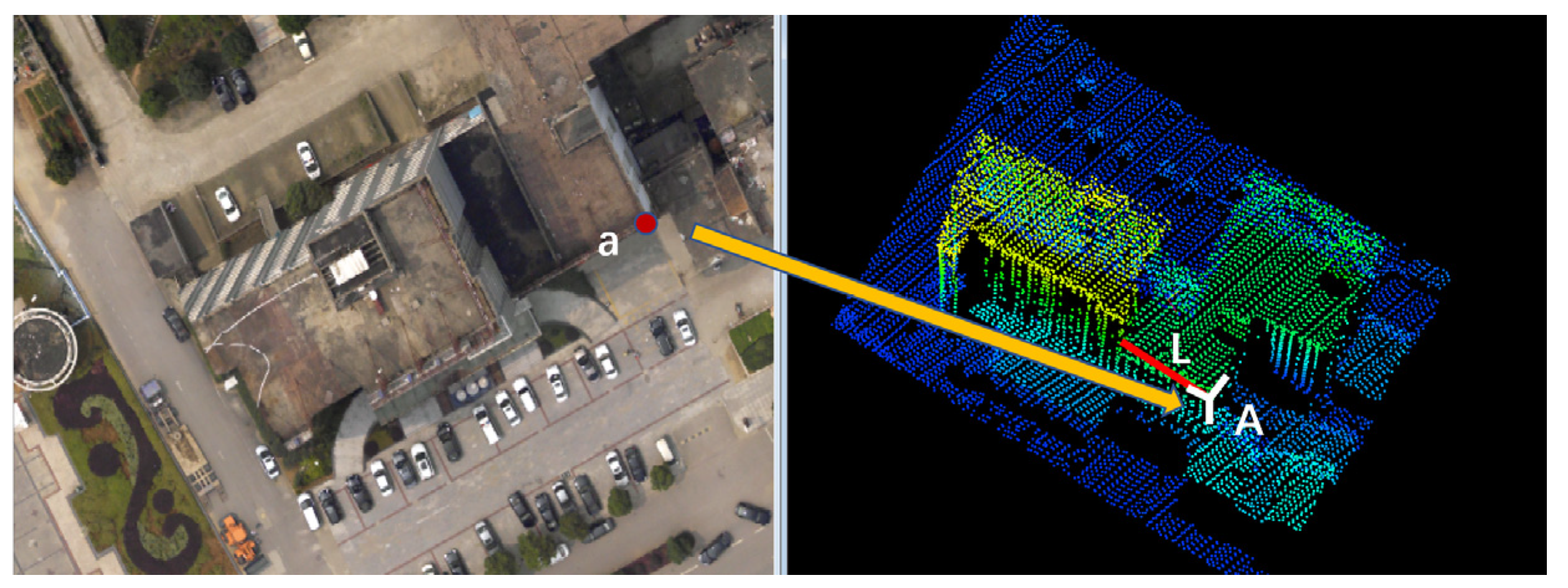
Figure 12.
The point ‘a’ on the image corresponds to the point A as the tie point. A cannot manually be selected on the laser point cloud. The point A is on the line L and L can be detected in the LiDAR data.

Figure 13.
The VP from the SL features.

Figure 14.
Curved roofs.

Figure 15.
The registration error when using VP as the registration primitive.

Figure 16.
Registration error chart in the image space (a) and LiDAR point space (b) respectively.

Figure 17.
Error distribution map.

Figure 18.
Lens distortion registration error influence of different camera type, including DMC, RCD105 and SWDC5. (a) DMC camera lens distortion registration error. (b) RCD105 camera lens distortion registration error. (c) SWDC5 lens distortion registration error.
Figure 18.
Lens distortion registration error influence of different camera type, including DMC, RCD105 and SWDC5. (a) DMC camera lens distortion registration error. (b) RCD105 camera lens distortion registration error. (c) SWDC5 lens distortion registration error.


Figure 19.
The influence of different feature types on the accuracy of the registration.


Table 1.
The comparation between LiDAR point cloud data and optical image [23].
Table 1.
The comparation between LiDAR point cloud data and optical image [23].
| LiDAR Point Cloud Data | Remote Sensing Image |
|---|---|
| Rich information on homogeneous surfaces | There is almost no positional information on homogeneous surfaces |
| Data can be obtained during the day and night | Most of the data can only be obtained during the day |
| Obtain accurate three-dimensional coordinates directly | Obtaining three-dimensional coordinates by matching process is complicated and unreliable matching results often occur |
| The vertical accuracy is better than the horizontal accuracy | The horizontal accuracy is better than the vertical accuracy |
| Highly redundant information | No inherent redundant information |
| Rich location information only, and it is difficult to extract semantic information | Rich semantic information |
Table 2.
The error characteristics of the point, line, and patch primitives in LiDAR data.
| Primitive Type | Error Description | Mathematical Expression Complexity |
|---|---|---|
| Point | Has the property of semi-random dispersion | |
| Patch | Relatively accurate, it is generated from the whole fitting of the same patch point cloud which depends on the patch segmentation accuracy | |
| Line | Line features are obtained by intersecting patches and the accuracy depends on the extraction accuracy of patches |
Table 3.
The details of the test data.
| Properties of the Data | Henan (Test Site 1) | Xuzhou (Test Site 2) | Xianning I (Test Site 3) | Xianning II (Test Site 3) |
|---|---|---|---|---|
| LiDAR Point Data | ||||
| Attitude of image (m) | 600 | 1500 | 1000 | 1000 |
| Points density (pts/m2) | 4 | 2.5 | 4.0 | 4.0 |
| Attitude of points (m) | 800 | 600 | 1000 | 1000 |
| LiDAR scanner type | Leica ALS 70 | A-Pilot | Leica ALS50 II | Leica ALS50 II |
| Acquisition time | 2018. 11 | 2014.6 | 2009.03 | 2009.03 |
| Image data | ||||
| Camera type | DMC | SWDC-5 | RCD105 | RCD105 |
| f (mm) | 120 | 35 | 35 | 35 |
| Overlap | 60% | 70% | 70% | 70% |
| CCD size (um) | 12 | 6.0 | 6.8 | 6.8 |
| Image resolution (m) | 0.06 | 0.15 | 0.1 | 0.1 |
| Acquisition time | 2018. 11 | 2014.6 | 2009.03 | 2009.03 |
| Original primitive type | Straight Line | Straight Line and Curve | Straight Line | Curve |
Table 4.
The information of the test sites (unit: pixel).
| Test Site 1 | Test Site 2 | Test Site 3 | Test Site 3 | |
|---|---|---|---|---|
| Primitive Type | Straight Line | Straight Line and Curve | Straight Line | Curve |
| Image number | 9 | 9 | 4 | 4 |
| Check points number | 30 | 30 | 15 | 15 |
| Average error (pixel) | 0.636 | 1.339 | 1.029 | 1.383 |
| Average error (m) | 0.0382 | 0.2 | 0.103 | 0.138 |
| Standard deviation | 0.288 | 0.615 | 0.781 | 0.670 |
Table 5.
Comparison of registration accuracy of different density LiDAR data (unit: pixel).
| 4 pt/m2 | 2 pt/m2 | |
|---|---|---|
| 1 | 0.894524 | 1.143759 |
| 2 | 0.971825 | 0.920501 |
| 3 | 0.429864 | 0.616121 |
| 4 | 0.107464 | 0.209425 |
| 5 | 0.300463 | 0.59597 |
| 6 | 0.207973 | 0.614754 |
| 7 | 0.768295 | 0.865744 |
| 8 | 0.097773 | 0.795144 |
| 9 | 0.749856 | 0.537697 |
| 10 | 0.897527 | 0.96451 |
| 11 | 0.897527 | 1.101736 |
| 12 | 0.300463 | 0. 474126 |
| 13 | 0.353553 | 0.354412 |
| 14 | 0.52452 | 0.546122 |
| 15 | 0.894524 | 0. 705083 |
| average | 0.5597 | 0.7128 |
Table 6.
The check points results of different primitive feature types (unit: pixel).
| Check Point | Linear Features | Curve Features |
|---|---|---|
| 1 | 0.463344 | 1.324443 |
| 2 | 2.047939 | 1.922908 |
| 3 | 0.361981 | 0.186339 |
| 4 | 0.549812 | 2.204933 |
| 5 | 1.718475 | 2.224358 |
| 6 | 0.001718 | 1.792193 |
| 7 | 0.044382 | 0.454203 |
| 8 | 0.010391 | 0.177646 |
| 9 | 1.979701 | 2.279956 |
| 10 | 0.463344 | 1.324443 |
| 11 | 0.745356 | 0.891393 |
| 12 | 1.975545 | 1.502313 |
| 13 | 1.798919 | 1.589025 |
| 14 | 1.795055 | 1.449832 |
| 15 | 1.476673 | 1.419629 |
| average | 1.0288 | 1.3829 |
Table 7.
The results of different registration methodology.
| Chunjing Yao | Bai Zhu [33] | Bisheng Yang [26] | |
|---|---|---|---|
| Image space (unit: pixel) | 0.636 | 1.798 | 1.876 |
| LiDAR data space (unit: m) | 0.0382 | 0.3596 | 0.3752 |
| Image resolution (unit: m) | 0.06 | 0.2 | 0.2 |
| Point density (pts/m2) | 4 | 6.91 | 25 |
| Image number | Single and multiple | Single and multiple | Multiple |
| Computational time | least | medium | most |
Publisher’s Note: MDPI stays neutral with regard to jurisdictional claims in published maps and institutional affiliations. |
© 2021 by the authors. Licensee MDPI, Basel, Switzerland. This article is an open access article distributed under the terms and conditions of the Creative Commons Attribution (CC BY) license (https://creativecommons.org/licenses/by/4.0/).
Share and Cite
MDPI and ACS Style
Yao, C.; Ma, H.; Luo, W.; Ma, H. A Precisely One-Step Registration Methodology for Optical Imagery and LiDAR Data Using Virtual Point Primitives. Remote Sens. 2021, 13, 4836. https://0-doi-org.brum.beds.ac.uk/10.3390/rs13234836
AMA Style
Yao C, Ma H, Luo W, Ma H. A Precisely One-Step Registration Methodology for Optical Imagery and LiDAR Data Using Virtual Point Primitives. Remote Sensing. 2021; 13(23):4836. https://0-doi-org.brum.beds.ac.uk/10.3390/rs13234836
Chicago/Turabian StyleYao, Chunjing, Hongchao Ma, Wenjun Luo, and Haichi Ma. 2021. "A Precisely One-Step Registration Methodology for Optical Imagery and LiDAR Data Using Virtual Point Primitives" Remote Sensing 13, no. 23: 4836. https://0-doi-org.brum.beds.ac.uk/10.3390/rs13234836
Note that from the first issue of 2016, this journal uses article numbers instead of page numbers. See further details here.