Desertification Extraction Based on a Microwave Backscattering Contribution Decomposition Model at the Dry Bottom of the Aral Sea

Abstract

The fine particles produced during the desertification process provide a rich material source for sand and dust activities. Accurately locating the desertified areas is a prerequisite for human intervention in sand and dust activities. In arid and semi-arid regions, due to very sparse vegetation coverage, the microwave surface scattering model is very suitable for describing the variation of topsoil property during the process of desertification. However, the microwave backscattering coefficient (MBC) trend of the soil during the desertification process is still unclear now. Moreover, the MBC of a resolution unit usually involves the contribution of soil and vegetation. These problems seriously limit the application of microwave remote sensing technology in desertification identification. In this paper, we studied the soil MBC change trend during the desertification process and proposed a microwave backscattering contribution decomposition (MBCD) model to estimate the soil MBC of a resolution unit. Furthermore, a simple microwave backscattering threshold (SMSBT) model was established to describe the severity of desertification. The MBCD and SMSBT models were verified qualitatively through landscape photos of sampling points from a field survey in November 2018. The results showed that the MBC would gradually decline with the deepening degree of desertification. The MBCD model and the corresponding least squares method can be used to estimate the soil MBC accurately, and the SMSBT model can accurately distinguish different degrees of desertification. The results of desertification classification showed that more than 68% of the dry bottom of the Aral Sea is suffering from different degrees of desertification.

1. Introduction

The United Nations Convention to Combat Desertification (UNCCD) defined desertification as land degradation in arid, semi-arid, and dry sub-humid areas resulting from various factors, including climatic variations and human activities [1,2,3,4,5,6,7,8]. The desertification process produces many sand and dust particle grains, providing rich material for sand and dust activities [9]. The Aral Sea region, one of the world’s worst disaster areas, is suffering from a rapid process of desertification. The sand and dust particles aroused from the dry bottom of the Aral Sea are rich in salt and toxic substances, resulting in both the widespread death of vegetation as well as various human diseases [10,11]. Location of desertification spatial distribution is a prerequisite for human intervention in the process of desertification. Due to the enormous advantages of remote sensing technology in desertification monitoring, researchers developed various methods based on remote sensing data and technology to identify the desertification process.

In 1998, Becker related the Normalized Difference Vegetation Index (NDVI) and Microwave Polarization Difference Index (MPDI) to monitor vegetation and desertification, suggesting the relationship between moisture and photosynthesis [12,13]. In other research, Albedo and NDVI were used as indicators to classify different degrees of desertification [14]. Currently, researchers developed a variety of desertification indicators, such as NDVI, Albedo, MSDI (Standard Deviation Index), shifting sand proportion, VFC (fraction of vegetation cover), modified soil-adjusted vegetation index (MSAVI), bare soil index (BSI), degradation index (DI), Soil Quality Index (SQI), Climate Quality Index (CQI), Vegetation Quality Index (VQI), Management Quality Index (MQI), Environmental Sensitive Areas Index (ESAI) and Bagnouls–Gaussen Aridity Index (BGI), and so on [4,6,15]. The spectral mixture analysis (SMA) method was first proposed by Collado in 2002 and was used to estimate the fraction of different land types coverage [16]. The use of the SMA method significantly improved the accuracy of the desertification area estimation [17]. Collado used least squares method to estimate the fraction of different land types. However, in a study dominated by Asner, another method based on probability was proposed to estimate the fraction of vegetation in the arid area [18]. In a case study of desertification in Africa, four indicators, including vegetation cover, rain use efficiency (RUE), surface run-off, and soil erosion, were used to monitor desertification [19]. In another case study, a simple machine learning method was used to extract potential areas with desertification risk [20]. Sun uses the cost-distance method to assess the risk of desertification, Lin established a fuzzy model to evaluate desertification, and Guo proposed a decision tree method to discriminate desertification [7,21,22]. Qiao extracted the desertification information based on an artificial neural network method, and the result shows that this method can reach up to an accuracy of 84% [23]. Jia used a decision tree method to extract the desertification information, Wei utilized the feature space combinations method to identify desertification, and Feng distinguished desertification based on an object-oriented classification method, and so on [24,25,26,27,28]. Silva used a method based on concepts of mathematical morphology, vegetation index and classification of digital images to distinguish desertification [29]. Moreover, the soil moisture from the satellite microwave estimation was often used for desertification studies [30].

According to the literature review above, identifying desertification mainly involves three methods: visual interpretation, desertification indicators, and machine learning, which provide a variety of ways for us to locate the desertification areas. However, these methods have more or fewer problems in practical applications. Due to the heavy workload, it is nearly impossible for us to use visual interpretation in extensive area desertification monitoring. In addition, the desertification indicators can hardly characterize the status of the desertification directly, and the indicator maps often have a relatively low spatial resolution due to the use of low spatial resolution satellite images in the process of calculating these indicators. To make matters worse, cloudy weather in some arid areas makes obtaining high-quality optical remote sensing data difficult. Because of the difficulty in labelling different levels of desertification, machine learning methods can hardly be used in desertification discrimination. The microwave remote sensing technology provides us with a powerful tool to describe the characteristics of the topsoil property changes in the desertification processes. Compared with optical remote sensing data, microwave remote sensing data is hardly affected by clouds and rain, and it has a relatively high spatial resolution. In addition, due to the difference in wavelength scale between microwave remote sensing and visible light remote sensing, microwave remote sensing technology can be used to distinguish changes of soil surface roughness during the desertification process, which cannot be distinguished in the visible light band. However, currently, there is nearly no relevant research using microwave remote sensing technology to describe desertification.

Soil particle size is a vital indicator during the desertification process, and it is well suited to characterize the extent of desertification. As the degree of desertification deepens, the particle size of the topsoil gets smaller and smaller, and the topsoil surface becomes smoother and smoother. However, this change in formation of the surface soil particle size can hardly be obtained from optical remote sensing data because nearly natural soil surfaces all look very rough in the visible light waveband. Fortunately, the backscattering of microwaves is very sensitive to the change of the ground surface particle size. When the particle size is relatively small, the surface looks very smooth for the microwave, and the scattering energy is concentrated in the mirror direction, so the backscattering energy is very weak. However, the backscattering energy will gradually get significant with the increase of particle size without considering the influence of permittivity, which has a close relationship with the salinity and moisture of the topsoil. In addition to the interference factor of permittivity, another problem always exists when using the microwave backscattering coefficient to describe the degree of desertification. The issue is that the backscattering coefficient of a resolution unit usually involves the contribution of soil and vegetation. However, what we need is the MBC of the soil of the resolution unit. Until now, we have not found any research involving the decomposition of backscattering contributions of soil and vegetation within a resolution unit, which led to the focus of this paper, including:

• The variation trend of the roughness and electrical roughness of the topsoil in the process of desertification, the evaluation of the effects of soil moisture and soil salinity on backscatter in arid and semi-arid regions, and whether the backscattering coefficient can be used to describe the degree of desertification.
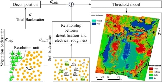
• Developing a model for decomposing the backscattering contribution of vegetation and soil within a resolution unit and estimating the backscattering coefficient of soil within this resolution unit.
• Use the backscattering coefficient of soil to assess the severity of desertification at the dry bottom of the Aral Sea.

2. Research Area

The Aral Sea is located between the two countries of Kazakhstan and Uzbekistan, lying in the hinterland of Eurasia, and it is far from the North Aral Sea. Thus, this region has a classical continental dry climate, and it provided favorable conditions for the spread of desertification. The temperature in this place can reach up to 40 °C in summer but may drop below −20 °C in winter. The average annual precipitation is only between 100 mm and 250 mm [11]. The relatively dry climate has exacerbated the process of desertification, and a new dessert, called Aralkum Desert, is taking shape. Currently, the Aral Sea’s exposed dry bottom is becoming a source of salts and chemicals, which are resources for adjacent areas. So, the storms here are often be called ‘salt-dust storms’. More and more research results suggest that the exposed dry bottom of the Aral Sea is becoming a new ‘hot spot’ of sand and dust storms [10,11,31]. The sand and dust activity usually occurs at the place where the desertification is severe. Thus, obtaining the spatial distribution of desertification areas with different severity is the first step for human intervention in sand and dust activities. The study area in Figure 1 indicates that the site is dominated by a large area of bare land, providing favorable conditions for desertification.

3. Data and Method

3.1. Data

3.1.1. Remote Sensing Data

Sentinel-1 SAR GRD is C-band Synthetic Aperture Radar Ground Range Detected with log scaling. The C-band Synthetic Aperture Radar wavelength is about 5.67 cm, and the azimuth and range resolution is 10 m. The MBC described in dB ranges from −50 dB to 0 dB, while the corresponding normalized backscattering coefficient is between 0 and 1. These two expressions have a simple relationship such as the following [32]:

$${\sigma }_{dB}=10{\log }_{10}{\sigma }_N$$

(1)

where ${\sigma }_{dB}$ denotes the backscattering coefficient in dB and ${\sigma }_N$ is the normalized backscattering coefficient. Because of weak volume scattering in arid and semi-aid area, VV polarization is selected for characterizing surface soil scattering features. The instrument model is set as Interferometry Wide (IW) with a descending orbit model, and the data was obtained from 23 June 2020 to 5 July 2020. These data can be easily accessed through the Google Earth Engine (GEE) platform (https://developers.google.com/earthengine/datasets/catalog/COPERNICUS_S1_GRD#description, accessed on 10 June 2021). Additionally, the data access code that we used in this paper can be easily found from this link: https://code.earthengine.google.com/0659c95cc2523eff71ed05c344a46b9e, accessed on 12 June 2021. This paper calculates the VFC by pixel dichotomy, which Li first proposed in 2004 [33]. Before Landsat 8 Collection 1 Tier 1 8-Day NDVI Composite were used to compute VFC, we tried to use surface reflectance of band four and band three of sentinel-2 Multispectral Instrument to obtain VFC. However, high-quality remote sensing data with little cloud during this period can hardly be found. To evaluate the influence of soil moisture and soil salinity on the SMSBT model, we also obtained the volumetric soil moisture data of the surface soil with a spatial resolution of about 10 km at a depth of 0–7 cm in the Aral Sea area. The soil moisture data was from the ERA5 data set, which is a reanalysis data set. The data and the corresponding data access code can also be easily found on the GEE platform.

3.1.2. Field Sampling Data

Landscape photos of 15 sampling points in the study area are used to analyze and verify the MBCD and SMSBT model. In 2018, researchers from China and Uzbekistan conducted a field survey of desertification in the Amu Darya Delta, and the landscape photos and soil salinity data originates from this field investigation. The useful information such as VFC and topsoil moisture for each sampling point can be visually estimated from the scene picture. These data will be used to qualitatively assess the potential of the SMSBT model to differentiate different levels of severity of desertification.

3.2. Methods

3.2.1. Simple Microwave Backscattering Threshold (SMSBT) Model

The process of desertification is closely related to the surface roughness changes. The surface roughness is usually characterized by electrical roughness, which is the product of the wavenumber and the root mean square height of the surface of the dielectric surface. The wavenumber $k$ and mean square height $s$ can be calculated by the following formula:

$$k=\frac{2\pi }{\lambda }$$

(2)

$$s=\sqrt{\frac{{{\displaystyle \sum }}_{n=1}^N{\left(h\left(n\right)-\overline{h}\right)}^2}{N-1}}$$

(3)

where $\lambda$ is the wavelength of electromagnetic waves, $N$ is the number of sampling points, $h\left(n\right)$ is the height of the $n\mathrm{th}$ sampling points, and $\overline{h}$ is the mean height of all sampling points. According to the study of Adib and Yisok, the backscattering coefficient from a rough dielectric surface increases as electrical roughness increases, and it saturates as electrical roughness exceeds 3 [34,35,36]. To relate the process of desertification with electrical roughness, we simply divide the desertification process into four stages, briefly indicating the change of root mean square height and roughness during the process of desertification. The desertification process is such as that shown in Figure 2.

Desertification is a process in which large stone, soil blocks and particles gradually decompose into little particles under rain and wind erosion. As mentioned in Section 2, the classical continental dry climate provides favorable conditions for wind erosion, such as relatively large temperature differences, sparse rainfall, and high wind speed. Under the wind and temperature differences, large rocks and soil blocks crack into smaller stones and smaller blocks. This process can be described by four scenarios (a–d) shown in Figure 2. To facilitate the analysis of the root mean square height and electrical roughness changes, the process of desertification is simplified, and only four scale particles are used to describe this process. The root mean square height and electrical roughness for C-band are calculated according to Formulas (2) and (3), respectively, and the results are shown in Figure 2. As shown in Figure 2, both the root mean square height and electrical roughness gradually decline as the degree of desertification deepens. From Figure 2a, we can find that only some relatively large stones sparsely distributed with an equivalent volume diameter of about 10 cm may produce an electrical roughness that excess 3. However, stones of this size seldom exist in arid, barren land around the Aral Sea, according to the topsoil samples obtained from the field survey. In addition to the situation assumed in Figure 2, another case may also exist. With the gradual increase of vegetation, the soil particle size will also gradually become smaller under the effect of vegetation on soil improvement. In this case, although the particle size of the soil will gradually decrease, the electromagnetic roughness obviously cannot reflect the degree of desertification. Fortunately, the vegetation cover for most of the arid and semi-arid areas is very sparse. Furthermore, the soil moisture in areas with high vegetation coverage is usually relatively high, which will significantly increase the backscattering coefficient of the soil. In fact, according to our common sense, the particle size of the soil in the high vegetation coverage area will not become as small as that of the sand in the desert, and the soil surface will not become as smooth as the desert. Based on the backscattering coefficient, these high vegetation coverage areas may still not be identified as desertified areas, and this case will be carefully discussed in the next part. Therefore, a backscattering coefficient can be used to describe the degree of desertification in the arid area, and the simple microwave backscattering threshold (SMSBT) model is proposed to describe the desertification process based on this theory.

In 2012, Nashashibi established a desert surface backscattering model, and the results indicated the backscattering coefficient was between −26 dB and −30 dB for s band in the desert area [34]. However, for the C-band, the backscatter coefficient should be slightly higher than this range. In fact, for bare land in arid and semi-arid regions, except for deserts, no land type can achieve such low backscatter values. Besides, some slight desertification areas can be found in the sampling points from the field survey, and the backscattering coefficient data can be easily found on the GEE platform. The model and data above can be used to determine the threshold of backscattering, and then the threshold will be used to describe the severity of desertification. In this paper, the Jenks method, field survey data and surface backscattering model are used to determine the threshold. Based on the analysis above, the SMSBT model described in Figure 3 is proposed to distinguish different degrees of desertification.

3.2.2. Influence of Soil Moisture and Salinity on the Uncertainty of the SMSBT Model

The performance of the SMSBT model for discriminating different levels of desertification will be affected by the soil permittivity, which is closely related to the moisture and salinity of the topsoil. In fact, for most arid and semi-arid regions, the moisture of the topsoil is so tiny that its effect on microwave backscattering may be almost negligible. Although some areas with high soil water content do exist, fortunately, both of the real and imaginary parts of the permittivity will increase significantly with the increase of water content, resulting in a significant rise in the backscattering coefficient, and these areas will not be identified as potential desertification areas by the SMSBT model [37]. In the arid and semi-arid areas, the real part of the permittivity of dry soil is usually between 2 and 4, and the imaginary part is generally less than 0.05 [37]. Furthermore, Nashashibi’s field investigation results showed that the real part of the dielectric constant of dry soil in arid areas is between 2.71–2.74, and the imaginary part is between 0.017–0.024, and both are very stable [34]. In addition, according to Halikainen’s experiment, when the soil volumetric water content is less than 5%, the real part of the soil dielectric constant is between 2–3, and the imaginary part of the soil dielectric constant is very close to 0, which is consistent with Nashashibi’s survey results [38]. The response of the backscatter to the permittivity change was tested in the case of different roughness. I2EM model for the single-scale random surface was used in this simple test, and the corresponding code can be found on the website of the book Microwave Radar and Radiometric Remote Sensing (website: https://mrs.eecs.umich.edu/codes/Module10_1/Module10_1.html, accessed on 22 June 2021). Results showed that slight fluctuation of dielectric constant could hardly lead to a significant change in the backscattering coefficient for different roughness. Therefore, when the soil moisture is lower than 5%, the influence of soil moisture on the dielectric constant and backscattering coefficient is almost negligible.

The salinity of the soil also significantly affects the dielectric constant of the soil, but this effect strongly depends on the volumetric moisture of the soil. According to Sreenivas’s study on the dielectric constant of salt-affected soil, the influence of soil salinity on the real part of the dielectric constant is negligible. When the volumetric moisture of the soil is less than 5%, the effect of soil salinity on the imaginary part of the dielectric constant is insignificant [39]. Since the imaginary part of the dielectric constant can be expressed as:

$${\epsilon }^{″}=\frac{\mu }{\omega {\epsilon }_0}$$

(4)

where $\mu$ is the conductivity of soil, $\omega$ is the angular frequency of the electromagnetic wave, and ${\epsilon }_0$ is the permittivity of the free space. Since electrical conductivity is proportional to the concentration of free ions in the soil, electrical conductivity has a positive correlation with soil salinity when soil moisture is constant. For the C-band, the frequency of electromagnetic waves is about 4–5 times that of 1.25 GHz, so the restriction that the effect of soil salinity on soil dielectric constant is negligible will be more relaxed. The analysis above means that for the C band, even if the volumetric moisture of the soil slightly exceeds 5%, the influence of soil salinity on the soil dielectric constant is still negligible. Therefore, when the volumetric soil moisture is lower than 5%, the backscattering coefficient mainly depends on the roughness of the topsoil, and the SMSBT model can be used to describe different degrees of desertification accurately.

Usually, the VFC will be relatively high in areas with high soil moisture, and these areas should be classified as reverse desertification areas according to our experience. For areas with high soil moisture, although their topsoil may not be as smooth as desert, its roughness may also be relatively small. Therefore, in this case, the roughness of the ground will no longer be suitable to describe the degree of desertification. Fortunately, as the soil moisture increases, the backscattering coefficient of the soil will also increase significantly. However, whether the soil backscattering coefficient in these areas is high enough that these areas can be classified as non-desertified areas is uncertain. For these regions, the uncertainty of the SMSBT model can be greatly reduced by quantitative analysis of the soil backscattering coefficient in the resolution unit, which will be discussed in the discussion part.

In conclusion, the model’s ability to distinguish different degrees of desertification is affected by soil moisture and soil salinity. The influence of soil salinity on the model will strongly depend on soil moisture. When the volumetric soil moisture is less than 5%, the influence of soil moisture and salinity on the model’s ability to describe different degrees of desertification may be negligible. When the soil moisture is higher than 5%, it is necessary to further quantitatively analyze the backscattering coefficients of different soil moisture to reduce the uncertainty of the model. The soil moisture data combined with the soil MBC will be used to further evaluate the impact of soil moisture and salinity on the model in the arid and semi-arid areas in Section 5.1. For bare land in arid and semi-arid regions, the land type within a resolution unit is usually not single, and the combination of vegetation and soil is the most common. If the SMSBT model is to be used to distinguish different degrees of desertification, the MBC of the soil must be separated from the total MBC of the resolution unit.

3.2.3. Microwave Backscattering Contribution Decomposition (MBCD) Model

In order to separate the MBC of the soil from the total MBC of the resolution unit, we assume that there are only soil and vegetation in the resolution unit. For bare land in arid and semi-arid regions, this assumption is usually reasonable [1]. As is shown in Figure 4, we assume that the area of vegetation and soil are $S_{veg}$ and $S_{soil}$ within a resolution unit, respectively, and the overall area of this resolution unit is $S$. The normalized backscatter coefficient of vegetation within this resolution unit is ${\sigma }_{veg}$, the normalized backscatter coefficient of soil within this resolution unit is ${\sigma }_{soil}$, and the normalized backscattering coefficient of the whole resolution unit is $\sigma$. The ${\sigma }_{veg}$, ${\sigma }_{soil}$ and $\sigma$ obviously satisfy the following relationship [37]:

$${\sigma }_{veg}{S}_{veg}+{\sigma }_{soil}{S}_{soil}=\sigma S$$

(5)

Dividing both sides of the Formula (5) by S leads to the following expression:

$${\sigma }_{veg}\frac{S_{veg}}{S}+{\sigma }_{soil}\frac{S_{soil}}{S}=\sigma$$

(6)

Since $S_{veg}+S_{soil}=S$, thus the Equation (6) above can be rewritten as:

$${\sigma }_{veg}\frac{S_{veg}}{S}+{\sigma }_{soil}\left(1-\frac{S_{veg}}{S}\right)=\sigma$$

(7)

$S_{veg}/S$ is the fraction of vegetation cover, and it can be replaced by $f_{veg}$. Thus, the relationship above can be written as:

$${\sigma }_{veg}{f}_{veg}+{\sigma }_{soil}\left(1-f_{veg}\right)=\sigma$$

(8)

According to the Equation (8) above, the MBC of vegetation and soil in the resolution unit satisfies a simple linear relationship. Generally, $\sigma$ is known, and $f_{veg}$ can be estimated by the pixel dichotomy [33]. So, ${\sigma }_{veg}$ and ${\sigma }_{soil}$ can be estimated by the least squares method.

3.2.4. MBC Estimation Based on Least-Squares Method

It is assumed that there are n sample points around the central point to be estimated, and these points can be used to estimate ${\sigma }_{veg}$ and ${\sigma }_{soil}$ of the central point. So, n linear equations can be used to estimate ${\sigma }_{veg}$ and ${\sigma }_{soil}$.

$$\begin{gathered} {\sigma }_{veg}{f}_{veg}^1+{\sigma }_{soil}\left(1-f_{veg}^1\right)={\sigma }_1 \\ {\sigma }_{veg}{f}_{veg}^2+{\sigma }_{soil}\left(1-f_{veg}^2\right)={\sigma }_2 \\ {\sigma }_{veg}{f}_{veg}^i+{\sigma }_{soil}\left(1-f_{veg}^i\right)={\sigma }_i \\ ⋮ \\ {\sigma }_{veg}{f}_{veg}^n+{\sigma }_{soil}\left(1-f_{veg}^n\right)={\sigma }_n \end{gathered}$$

(9)

The above system of equations can easily be rewritten in the form of a matrix.

$$\left[\begin{array}{cc}\begin{array}{c}{f}_{veg}^1\\ \begin{array}{c}{f}_{veg}^2\\ ⋮\\ \begin{array}{c}{f}_{veg}^i\\ \begin{array}{c}⋮\\ f_{veg}^n\end{array}\end{array}\end{array}\end{array}& \begin{array}{c}1-f_{veg}^1\\ \begin{array}{c}1-f_{veg}^2\\ \begin{array}{c}⋮\\ \begin{array}{c}1-f_{veg}^i\\ \begin{array}{c}⋮\\ 1-f_{veg}^n\end{array}\end{array}\end{array}\end{array}\end{array}\end{array}\right]\left[\begin{array}{c}{\sigma }_{veg}\\ {\sigma }_{soil}\end{array}\right]=\left[\begin{array}{c}{\sigma }_1\\ \begin{array}{c}{\sigma }_2\\ ⋮\end{array}\\ \begin{array}{c}{\sigma }_i\\ ⋮\\ {\sigma }_n\end{array}\end{array}\right]$$

(10)

Let $F$ be the vegetation coverage matrix (VCM), ${\sigma }_x$ be the backscattering decomposition matrix (BDM), $\mathsf{\sigma }$ be the backscattering composite matrix, and make the following conventions:

$$F=\left[\begin{array}{cc}\begin{array}{c}{f}_{veg}^1\\ \begin{array}{c}{f}_{veg}^2\\ ⋮\\ \begin{array}{c}{f}_{veg}^i\\ \begin{array}{c}⋮\\ f_{veg}^n\end{array}\end{array}\end{array}\end{array}& \begin{array}{c}1-f_{veg}^1\\ \begin{array}{c}1-f_{veg}^2\\ \begin{array}{c}⋮\\ \begin{array}{c}1-f_{veg}^i\\ \begin{array}{c}⋮\\ 1-f_{veg}^n\end{array}\end{array}\end{array}\end{array}\end{array}\end{array}\right],{\sigma }_x=\left[\begin{array}{c}{\sigma }_{veg}\\ {\sigma }_{soil}\end{array}\right],\sigma =\left[\begin{array}{c}{\sigma }_1\\ \begin{array}{c}{\sigma }_2\\ ⋮\end{array}\\ \begin{array}{c}{\sigma }_i\\ ⋮\\ {\sigma }_n\end{array}\end{array}\right]$$

(11)

Then the linear equation system in matrix form can be succinctly expressed as:

$$F{\sigma }_x=\sigma$$

(12)

And the least squares estimate of ${\sigma }_x$ can be expressed as:

$$\widehat{{\sigma }_x}={\left(F^{T}F\right)}^{-1}{F}^T\sigma$$

(13)

3.2.5. Tips about Soil MBC Estimation

When the least squares method is used to estimate soil MBC, the distance and VFC difference between sampling points and the central point should be limited to reduce the estimation error. The estimation process and the problems can be explained with the help of Figure 5.

As is shown in Figure 5, if N sample points within the circular buffer of point $\left(i_0,j_0\right)$ are used to estimate BDM, the buffer radius can neither be too large nor too small. If the R is too large, the soil properties of the points far from the central point may be very different from that of the central point, and the estimated result could not denote the scattering characteristics of soil and vegetation of the central point. At the same time, if R is too small, there will not be enough points to estimate the BDM, and the estimated result will also not be accurate. Besides, suppose the vegetation coverage difference between the sample point and the central point is significant, the difference in soil properties between the two points may also be significant, which will also cause the inaccuracy of the BDM estimation. On the contrary, if the difference in VFC between the sample point and the central point is slight, it will be very likely to cause the linear correlation of some linear equations in VCM. Then the estimation of BDM will produce significant errors. So, the vegetation coverage of any two points should not be too small to avoid the singular matrix generated in the process of BDM estimation. Based on the analysis above, two rules during BDM estimation should be used to reduce the error, and the two rules are shown in Figure 5. According to the landscape photos of sampling points, the radius of the buffer area should be less than 100 m. In order to obtain enough points to estimate BDM of the central point, the radius is set as 100 m. Meanwhile, the absolute value of VFC difference for any two sampling points is limited between 0.05 and 0.2. This limitation can avoid the occurrence of a singular matrix and make the BDM better represent the scattering characteristics of the estimated points.

$$\begin{gathered} \mathrm{Rule}1:R=100\mathrm{m} \\ \mathrm{Rule}2:0.05\le \left|f\left(i,j\right)-f\left(h,k\right)\right|\le 0.2 \end{gathered}$$

(14)

4. Results

4.1. The Spatial Distribution of Soil Moisture and Salt-Rich Soil in Study Area

The vast area and the very harsh geographical environment in some regions make it very difficult to obtain the spatial distribution of soil salt in the entire Aral Sea area through field sampling. The source of salt in the topsoil of the Aral Sea is mainly the salt of the its own seawater. When the water disappears, the salt is deposited in the soil, forming the salt-rich soil. Therefore, the dry bottom of the Aral Sea should be rich in salt, and this place may be the main distribution area of the salt-rich soil in the Aral Sea. Satellite images from Google Earth from 1973 to 2020 were used to determine the historical dry bottom of the Aral Sea. Figure 6 shows the changes of the water body of the Aral Sea from 1973 to 2020, and the water body boundaries of 1973 and 2020 can be used to determine the dry bottom of the Aral Sea.

The soil salinity data of the sampling points from a field survey about the Aral Sea desertification in November 2018 were used to verify our inference that the soil at the bottom of the Aral Sea is rich in salinity. The location, time, and soil salt of sampling sites are shown in

Table 1. The soil salinity and electrical conductivity of sampling points at dry bottom of Aral Sea.

Site	Sample	Date	Soil Depth (cm)	Conductivity (µs/cm)	Total Salt (mg/g)
U5	us19	22 November 2018	0–5	39.875	119.275
	us20		5–10	20.300	61.400
U6	us23		0–5	18.770	54.350
	us24		5–10	13.490	38.075
U7	us30	23 November 2018	0–5	20.300	63.800
	us31		5–10	5.275	15.950

.

The soil salt sampling data in Table 1 show that the dry bottom of the Aral Sea is rich in salt. For sampling point U5, the ground surface is dominated by salt crust, and the topsoil salt reaches up to 119.275 g/g, which is a relatively high soil salt level. Although the soil salinity of sampling points U6 and U7 are not as high as that of sampling point U5, they still have a relatively high soil salinity level. The soil salinity of sampling point U6 is slightly lower than that of sampling point U7, which is probably the result of soil improvement by Haloxylon trees. French scientists planted a large number of Haloxylon trees near U6 to improve the soil in the area.

The volumetric soil moisture of the Aral Sea is shown in Figure 7. As shown in Figure 7, the red line is the rough boundary of the Aral Sea water surface in 1973. Since the dry bottom of the Aral Sea is the main distribution area of salt-rich soil, and the influence of soil salinity on the soil permittivity is strongly dependent on soil moisture, we made simple statistics on the soil moisture of the dry bottom of the Aral Sea. Besides, we also counted the soil moisture of some areas outside the range of the dry bottom of the Aral Sea. These data will be used to evaluate the influence of soil moisture and soil salinity on our models.

As was shown in Figure 7, The soil moisture is very low throughout the dry bottom of the Aral Sea. However, the soil moisture is relatively high in areas A, B, C, D, E and F. The soil moisture from some regions even exceeds 20%. In these areas with high volumetric soil moisture, only areas D and E belong to the dry bottom of the Aral Sea, and the other areas with high soil moisture are all not within the range of the dry bottom of the Aral Sea. Statistical results of soil moisture at the dry bottom of the Aral Sea in Figure 7b indicated that only a few areas have soil moisture above 5%, and the soil moisture of most places is below 5%. The two peaks of soil moisture are distributed between 0.8% to 1.2% and 2.4% to 2.8%, respectively. The areas with soil moisture lower than 3% accounted for 91.95% of the dry bottom of the Aral Sea, the areas with soil moisture lower than 5% accounted for 96.81% of the dry bottom of the Aral Sea, and the areas with soil moisture lower than 7% accounted for 97.99% of the dry bottom of the Aral Sea. The statistical results also show that the soil moisture is the lowest from May to October throughout the year. Except for area E, the soil moisture for other areas with high soil moisture is nearly all above 10% from May to October. The soil moisture of area E from May to October is about 6%, and it is less than 6% from June to August.

4.2. Backscattering Coefficient and VFC in the Aral Sea

As mentioned in Section 3, Sentinel-1 SAR GRD data with VV polarization, IW and descending pattern from 23 June 2020 to 5 July 2020, was obtained to derive the MBC of soil and vegetation in an independent resolution unit (Figure 8b). Under normal circumstances, bare land, grassland, forest and shrub areas are areas where desertification may occur. The land type data with a resolution of 10 m from Tsinghua University are used to extract potential desertification areas based on GIS-based method (land type data: http://0-data-ess-tsinghua-edu-cn.brum.beds.ac.uk/, accessed on 22 June 2021), which means that other land types such as impervious land surface, water, wetland, and snow/ice area were removed from the study area. The VFC data was calculated by Landsat 8-day NDVI from 23 June 2020 to 5 July 2020. Because the VFC in some parts of the south of the Aral Sea is nearly equal to 1 where the vegetation cover is dense, the NDVI of vegetation and soil is set as the maximum and minimum value of NDVI, respectively. The process of finding the extreme value of NDVI in the study area was finished on Google Earth Engine (GEE) platform, where you can easily find the data that you need and the corresponding codes to access the data. The NDVI of vegetation and soil is set as 0.736 and 0, respectively, and the calculation result of VFC is shown in Figure 8a.

As is shown in Figure 8a, the average value of VFC in the Aral Sea is 0.1264, indicating a shallow vegetation cover in the study area. The VFC is between 0 and 0.10 for 50% of the study area, between 0.1 and 0.25 for 46% of the study area, and between 0.25 and 0.50 for 3% of the study area. Vegetation coverage data shows that about 85% of the land in the study area is barren in arid and semi-arid regions according to International Geosphere-Biosphere Programme (IGBP) classification standards. According to Figure 8b, the mean value of the backscattering coefficient is −16.6425 dB after removing water, wetland and impervious surface from the study area. However, the backscattering coefficient involves the contributions of both vegetation and soil within a resolution unit. This value cannot be used to characterize the desertification until the backscattering coefficient of soil is decomposed from the total backscattering coefficient of the resolution unit.

4.3. Backscattering Coefficient of Soil and the Landscape Photos of Sampling Sites

The backscattering coefficient of soil was estimated by the least-squares method under the rules described in Section 3.2.5, and the result was shown in Figure 9a. It must be noted that both the vegetation coverage and the backscattering coefficient are resampled to 50 m to greatly reduce the amount of calculation in the MBC estimation process, and parallel computing combined with GPU acceleration can also shorten the time of the MBC estimation to a certain extent. The quality improvement (QI) was proposed to assess the effect of the MBCD model, and it can be expressed as:

$${\mathrm{QI}}^{dB}={\sigma }_{soil}^{dB}-{\sigma }^{dB}$$

(15)

where ${\sigma }^{dB}$ is the total backscattering coefficient (described in dB) of a resolution unit, ${\sigma }_{soil}^{dB}$ denotes the backscattering coefficient (described in dB) of soil within this resolution unit, and ${\mathrm{QI}}^{dB}$ is the quality improvement (described in dB). The Aral Sea’s quality improved map (QIM) was shown in Figure 9b. Since it is difficult to obtain the true backscattering coefficient of the soil in the resolution unit, it is very difficult to verify the MBCD model quantitatively. We can only use the QIMs and the landscape photos of the sampling points to evaluate qualitatively the correctness of estimation results by the model. Therefore, four typical areas were selected to assess the MBCD model qualitatively, including sampling points L12, L14, L15 and X. However, we do not have the corresponding landscape photos of X, so we use satellite images of area X instead of landscape photos. The landscape photos, satellite images and QIMs of these sampling points can also be found in Figure 9.

According to Figure 9a, the mean value of the backscattering coefficient of soil is −16.5667 dB, indicating the fairly low level of soil backscattering in the Aral Sea. The value of soil backscattering coefficient between −41 dB and −17 dB for about 54% of the study area. Through the landscape photos of L12, we can find that relatively severe desertification has occurred in this area. The soil backscattering coefficient of L12 is about −17 dB (Figure 9), which may indicate that more than 54% of the land in the Aral Sea has been desertified. Due to the very sparse vegetation fraction cover in the study area where VFC is lower than 0.25 for 96% of the region, the backscattering coefficient of the soil in most areas has slightly increased relative to the total backscattering coefficient. However, there are also some areas, such as the areas with buildings in them and the areas with high soil moisture, where the backscattering coefficient of the soil has increased significantly. To better evaluate the MBCD model, we related Equations (15) and (8), and then QI (described in dB) can be rewritten as:

$$\mathrm{QI}=10\lg {\sigma }_{soil}-10\lg \sigma =10\lg \frac{\frac{{\sigma }_{soil}}{{\sigma }_{veg}}}{f_{veg}+\left(1-f_{veg}\right)\frac{{\sigma }_{soil}}{{\sigma }_{veg}}}$$

(16)

where ${\sigma }_{soil}$ is the normalized backscattering coefficient of soil within a resolution unit, ${\sigma }_{veg}$ is the normalized backscattering coefficient of vegetation within this resolution unit, and $\sigma$ is the total normalized backscattering coefficient of this resolution unit. The relationship between QI and ${\sigma }_{soil}/{\sigma }_{veg}$ for different levels of $f_{veg}$ was depicted in Figure 10, and the results clearly showed what kind of land types can yield a high-level QI and what land types may produce a low-level QI.

Before analyzing the relationship between QI and ${\sigma }_{soil}/{\sigma }_{veg}$ for different levels of $f_{veg}$, three typical areas were used to estimate ${\sigma }_{soil}$ and ${\sigma }_{veg}$, and the value of which will significantly help us understand some results depicted in Figure 10. A buffer with a diameter of 100 m is established for each sampling point, and it will be used to estimate ${\sigma }_{soil}$ and ${\sigma }_{veg}$. This process was finished on the GEE platform, and the landscape photo for each sampling point and the corresponding estimated results were shown in Figure 11. As is shown in Figure 11a,c, the soil backscattering coefficient of the desertification area is very close to the value of the vegetation backscattering coefficient. According to the relationship between desertification degree and backscattering coefficient, if the soil backscattering coefficient is lower than that of vegetation, the desertification degree will be more serious than that shown in sampling point L2, and the foliage will be sparser. However, when the soil backscattering coefficient is higher than the vegetation backscattering coefficient, the vegetation coverage may be relatively high or low, and its value range is between 0–1. For example, the backscattering level of sampling point L14 is very high, but its VFC is close to 0. When the soil moisture in the high vegetation coverage area is very high, or there are artificial buildings in the high vegetation coverage area, the backscatter level of the soil will also be very high.

Once the soil backscattering coefficient is separated from the total backscattering coefficient, it can be used to describe the severity of desertification. In the next part, the SMSBT model will be used to classify the degree of desertification.

4.4. Results of Desertification Classification and Landscape Photos of Sampling Sites

The soil backscattering coefficient within a resolution unit was used to describe the degree of desertification based on the SMSBT model. During the process of determining the threshold, firstly, the Jenks method was used to divide soil backscattering coefficient (SBC) into five categories, representing different degrees of desertification, named leve1 ($-11.5\mathrm{dB}<\mathrm{SBC}\le 0\mathrm{dB}$), leve2 ($-14.8\mathrm{dB}<\mathrm{SBC}\le -11.5\mathrm{dB}$), leve3 ($-17.0\mathrm{dB}<\mathrm{SBC}\le -14.8\mathrm{dB}$), leve4 ($-19.8\mathrm{dB}<\mathrm{SBC}\le -17.0\mathrm{dB}$), leve5 ($\mathrm{SBC}\le -19.8\mathrm{dB}$). To determine the threshold for distinguishing desertification from non-desertification, we conducted a statistical analysis of desertification region L12. The result shows that the backscattering coefficient of this region is a random variable with approximately normal distribution. The upper bound of the 68% confidence interval (about −14.6 dB) is used as the threshold to distinguish desertification and non-desertification areas more accurately. After a simple modification, SBC can be reclassified into four categories to describe the severity of desertification, including no desertification ($-14.6\mathrm{dB}<\mathrm{SBC}\le 0\mathrm{dB}$), slight desertification ($-17.0\mathrm{dB}<\mathrm{SBC}\le -14.6\mathrm{dB}$), moderate desertification ($-19.8\mathrm{dB}<\mathrm{SBC}\le -17.0\mathrm{dB}$), and severe desertification ($\mathrm{SBC}\le -19.8\mathrm{dB}$). The classification result is shown in Figure 12.

Although the UNCCD has defined desertification, there is no unified classification standard, so it isn’t easy to describe the degree of desertification through quantitative sampling data. Therefore, the desertification classification results are hard to validate quantitatively, and we can only qualitatively judge the degree of soil desertification based on the soil conditions on the ground. Therefore, landscape photos obtained from a field survey are used to verify the classification results qualitatively. Because this field survey was not designed for this study, not all sampling points are within the scope of the study area. Finally, we selected all sampling points within the study area, and these sampling points can represent almost all land types in the area. Fifteen landscape photos and the corresponding pixel-scale (DCMs) of sampling points are used to validate the desertification classification results. These data can be found in Figure 13.

5. Discussion

5.1. The Influence of Soil Moisture and Soil Salinity on the SMSBT Model in the Study Area

According to the Microwave surface backscattering model, the influence of soil moisture and soil salinity on the backscattering coefficient is mainly reflected in their influence on the soil dielectric constant, and the impact of soil salinity on the soil dielectric constant strongly depends on the soil moisture [37]. In this part, the influence of soil moisture and soil salinity on soil dielectric constant will be divided into two parts to discuss separately.

5.1.1. The Influence of Soil Moisture on the SMSBT Model

As is described in Figure 7, the areas with soil moisture lower than 5% accounted for 96.81% of the dry bottom of the Aral Sea, and only area D and area E are within the range of the Aral Sea’s dry bottom. The soil moisture in areas A, B, C, and F is also relatively high and even exceeds 20% for some areas, and these areas do not belong to the dry bottom of the Aral Sea. According to the analysis in Section 3.2.2, when the soil moisture exceeds 5%, the influence of soil moisture on the soil dielectric constant will become very significant. The results of Halikainen’s research indicate when the soil moisture exceeds 10%, the real part of the soil dielectric constant exceeds 5 [38]. However, the imaginary part of the soil increases slightly, at still less than 0.5. When the soil moisture reaches up to 20%, the real part of the dielectric constant will exceed 10, and the imaginary part of the dielectric constant is between 2 and 2.5. As the real and imaginary parts of the permittivity increase, the backscattering coefficient will also increase significantly, which may affect the model’s ability to describe the particle size of the surface soil. The results of numerous studies have shown that when the soil moisture exceeds 10%, the starting wind speed of sand particles will increase significantly, and even high wind speeds are difficult to blow particles from the ground into the air [40,41,42,43]. Therefore, these areas with soil moisture exceeding 10% can hardly be classified as desertified areas. The satellite image of sampling point X and the corresponding QIM in Figure 9 showed that the backscattering coefficient of the soil with high soil moisture improved by 5–24 dB relative to the entire resolution unit. According to Figure 10, the backscattering coefficient of vegetation is about −17 dB. Therefore, the backscattering coefficient of soil with high soil moisture should not be lower than −12 dB. According to the desertification classification standard in Figure 12, area X should belong to a non-desertification area, which indicates that the high soil moisture nearly has no influence on the SMSBT model. However, it must be noted that area X is an area with very high soil moisture, so this result shows that the model’s ability to describe desertification in areas with very high soil moisture is hardly affected by soil moisture. According to the estimation results of the soil backscattering coefficient in Figure 9, the soil backscattering coefficients of areas B and C, marked in Figure 7, are −15.4 dB, −13.2 dB, respectively, and these areas were respectively classified as slight desertification and non-desertification (Figure 12). However, since the soil moisture in these areas is around 10%, these areas should not be desertification areas. The misclassification results of regions B indicate that when the soil moisture is between 5–10%, the model may produce slight classification errors. The misclassification of desertification in areas B is probably due to the limited effect of low soil moisture on the backscattering coefficient. This slight effect of relatively low soil moisture cannot make the backscattering coefficient of the soil high enough that this area can be classified as a non-deserted area. In conclusion, when the soil moisture is lower than 5%, the influence of soil moisture on the SMSBT model can be ignored; when the soil moisture is between 5–10%, the model will produce a slight classification error; when the soil moisture is higher than 10%, the influence of soil moisture on the model will gradually disappear as the soil moisture increases.

5.1.2. The Influence of Soil Salinity on the SMSBT Model

In the study area, the influence of soil salinity on the dielectric constant may be negligible. As described in Section 4.1, the main source of salt in the Aral Sea is the saltwater of the Aral Sea, and the soil at the bottom of the dry Aral Sea should be rich in salt. In Table 1, the survey results of the soil salinity of the sampling points at the bottom of the dry Aral Sea confirm our inference. However, this field survey was not specifically designed for this study, so soil salinity was measured at only a few sites at the dry bottom of the Aral Sea, and the investigators did not measure the salinity of the soil outside the range of the dry bottom of the Aral Sea. Without the source of salt, the soil salinity outside the range of the dry bottom of the Aral Sea should be very low, so the influence of soil salinity on the dielectric constant in these areas may also be negligible. According to the analysis in Section 3.2.2, the influence of soil salinity on the real part of the dielectric constant is negligible for different soil moistures. The impact of soil salinity on the imaginary part of the dielectric constant strongly depends on the soil moisture. When the soil moisture is lower than 5%, the influence of soil salinity on the dielectric constant for different types of soils is also negligible. The results of the Aral Sea soil moisture statistics in Figure 7 show that soil moisture for more than 96% of the Aral Sea’s dry bottom is less than 5%. Therefore, the influence of soil salinity on the dielectric constant at the dry bottom of the Aral Sea can be ignored. For area D, where the soil moisture exceeds 10%, the MBC will increase significantly under the influence of soil moisture and soil salinity. As analyzed in Section 5.1, when the soil moisture of an area exceeds 10%, this area should not be a desertification area. According to the desertification classification results in Figure 12, most areas of region D are classified as non-desertified areas. The results indicate that when the soil moisture exceeds 10%, the soil salinity can increase the accuracy of the SMSBT model.

5.2. Assessment of the Estimation Results of the Soil MBC within a Resolution Unit

In Section 4.3, we obtained the estimation result of the soil backscattering coefficient within a resolution unit. QI was proposed and calculated to evaluate the correctness of the estimation results of the soil backscattering coefficient in the study area. Based on the results in Section 4.3, the relationship between QI and ${\sigma }_{soil}/{\sigma }_{veg}$ can be used to assess the estimation results of soil MBC within a resolution unit in the following cases:

• ${\sigma }_{soil}\le {\sigma }_{veg}$

When ${\sigma }_{soil}\le {\sigma }_{veg}$, land type would most probably be a desertification area such as that in Figure 9 (landscape of L12) and Figure 11a (landscape of L2), and $f_{veg}$ should be very close to 0. So, QI will be approximately equal to 0 according to Formula (16). As shown in the landscape photo and QIM of L12, $f_{veg}$ is close to 0, and QI is between 0 dB and 1 dB. Therefore, QIM of L12 and the corresponding landscape photo in Figure 9 are in good agreement with the inference above, indicating that when soil backscattering coefficient is lower than vegetation backscattering coefficient, the MBCD model is correct.

2.

${\sigma }_{soil}\ge {\sigma }_{veg}$, $f_{veg}\le 0.05$

The land type of L14 described in the landscape photo of Figure 9 satisfy this condition. As is shown in the landscape photo of L14, $f_{veg}$ is also very close to 0. Thus, QI will also be approximately equal to 0 according to Formula (16). According to the QIM of L14 in Figure 9, QI is between 0 and 1. This result coincides well with the above analysis, proving that when the soil backscattering coefficient is higher than the vegetation backscattering coefficient and the VFC is very close to 0, the MBCD model is also correct.

3.

${\sigma }_{soil}\ge {\sigma }_{veg}$, $0.05<f_{veg}\le 0.25$

Except for desertified areas, most of the study areas meet this restriction. As was shown in Figure 10, QI is between 0 dB and 1 dB when $f_{veg}$ ranges from 0.05 to 0.25. Therefore, QI should range from 0 dB to 1 dB for most of the study area. As is shown in Figure 9b, QI does range from 0 dB to 1 dB for most of the study area. Therefore, the model is still correct under this condition.

4.

${\sigma }_{soil}\ge {\sigma }_{veg}$, $f_{veg}>0.25$

Two actual surface scenes meet this condition: a human settlement area and a dense vegetation cover area. L16 is a representation of human settlements, and high vegetation coverage combined with the presence of strong scatterers (soils that are rich in water) are typical characteristics of this kind of area. According to Formula (16) and Figure 9, when ${\sigma }_{soil}$ is much higher than ${\sigma }_{veg}$ and $f_{veg}$ exceeds 0.25, QI should be higher than 1 dB. Furthermore, if ${\sigma }_{soil}/{\sigma }_{veg}$ is higher than $10$ and $f_{veg}$ exceeds 0.75, QI will rise to the range from 5 dB to 24 dB. As was shown in the landscape photo of L16 in Figure 9, high VFC and the existence of buildings will lead to a significant increase in QI. As is shown in the corresponding QIM of L16 in Figure 9, QI falls into the range from 1 dB to 5 dB for some pixels and from 5 dB to 24 dB for some other pixels as we inferred above.

Site X is an example of a dense vegetation area, where very dense vegetation coverage and strong scatterers (soils that are rich in water) usually exist. As is shown in the Google map of site X, very dense vegetation can be found here, and the ground surface soil is rich in water. Based on a visual interpretation, $f_{veg}$ exceeds 0.5 for most of the pixels around site X and exceeds 0.70 for some pixels around site X. According to Formula (16) and Figure 9, if ${\sigma }_{soil}/{\sigma }_{veg}$ is higher than 10, and $f_{veg}$ is higher than 0.5 but lower than 0.75, QI will fall into the range from 3 dB to 6 dB. When ${\sigma }_{soil}/{\sigma }_{veg}$ is higher than 10, and $f_{veg}$ is higher than 0.75, QI will range from 6 dB to 24 dB. According to the QIM of X, QI is between 1 dB and 24 dB for most of the pixels, indicating the correctness of the MBCD model.

Based on the validation by true ground surface showed in landscape photos of sampling points, the QI is in good agreement with the soil conditions shown in landscape photos of sampling points. These results show that the estimation of soil backscattering is correct after the use of the MBCD model. The soil moisture in areas A and F exceeds 15%, but these areas’ average backscattering coefficient is below −18 dB, which is obviously a wrong estimation result. According to our survey of these areas, relatively high vegetation coverage or relatively uniform spatial distribution of vegetation may be the main reason for the error in estimating the soil backscattering coefficient in this area. Because when the vegetation coverage is high, or the spatial distribution of vegetation is relatively uniform, the VFC of the sample points in the buffer will be very close to each other, and the least squares method will not accurately estimate the backscattering coefficient of the soil. Therefore, for some areas with high vegetation coverage or relatively uniform spatial distribution of vegetation, the model may fail to estimate the backscattering coefficient of the soil accurately.

5.3. Evaluation of the Results of the Desertification Classification

For the dry bottom of the Aral Sea, the DCMs and the corresponding landscape photos of 15 sampling points were used to evaluate the accuracy of desertification classification qualitatively. The results show that the DCMs are in good agreement with the actual degree of desertification at sampling sites. As was demonstrated in landscape photos of L6, L9, L15 and L16 in Figure 13, these places were all covered with relatively dense vegetation, and the soil here looks rather rough. Based on visual interpretation, no desertification signs are found in these places. The corresponding DCMs of these places indicate that these places are not to be classified as desertification areas. The consistency of the visual interpretation and the classification results of the SMSBT model suggests the model’s accuracy. Although nearly no vegetation was found in L14 and U7, the existence of large amounts of rocks with relatively large size directly showed that both L14 and U7 are not desertification areas. As is shown in the DCMs of L14 and U7, these sites are also classified as no desertification areas. So, the interpretation results are also in good agreement with the classification results of L14 and U7. As was shown in landscape photos of L10 and L12 in Figure 13, relatively large soil particles are not found in L10 and L12. However, these places are classified as no desertification areas. The inconsistency between visual interpretation results and SMSBT model classification results are most probably due to the high water content of the soil in these places, which was shown in the details of landscape photos of L10 and L12. However, the cause of high soil moisture for L10 and L12 may be different. The high soil moisture in L10 may be related to the short distance between L10 and waters. While the high water content of the soil in L12 may be related to the precipitation during the time interval for data acquisition. In some arid areas covered by low and sparse vegetation, the ground shows a slight trend of desertification, such as L7, L8, L11 and L5. Except for site L8, the visual interpretation results are consistent with the classification results of the SMSBT model. This inconsistency between visual interpretation and classification results of L8 may be due to a calculation error (as described in Section 5.2), visual interpretation error, or the change of soil property (field surveys were completed about a year and a half before SAR data were acquired). According to the landscape photos of L13, U5 and U6, there is a severe desertification trend in these areas, and these places are also classified as no desertification areas.

However, for areas outside the dry bottom of the Aral Sea, we can only use soil moisture data to verify the classification results of desertification because there is no sampling data. The soil moisture map in Figure 7c shows that the annual soil moisture in area A is above 10%, which should be a non-desertification area. However, the classification results in Figure 12 indicate that the area was misclassified as a moderately and severely desertified area. The misclassification of area A is probably due to our program settings in the SBC estimation process. Because when the VFC of the sample points in the buffer are very close to each other, the least squares method may fail to estimate the soil backscattering coefficient accurately. In this case, the soil backscattering coefficient is set as the backscattering coefficient of the entire resolution unit. Therefore, if the spatial distribution of vegetation in area A is very uniform, the VFC of sampling sites will be very close to each other, and the backscattering coefficient of the soil in this area will be estimated as the backscattering coefficient of the entire resolution unit. Furthermore, suppose the vegetation coverage in the area is relatively high. In that case, the backscatter coefficient of the soil in area A will be estimated as the backscatter coefficient of the vegetation in the area. According to the vegetation backscattering coefficient estimation results in Figure 11, the backscattering coefficient of vegetation is very close to that of desertified soil. Therefore, when the VFC of area A is very high, and the vegetation spatial distribution is highly uniform, the area is likely to be misclassified as a medium or even severe desertification area. According to our analysis of satellite images in this area, both areas A and F are human settlements. The artificial forests in this area may be the main cause for the error in estimating the soil backscattering coefficients of these areas. According to the soil moisture map in Figure 7, areas B, C, and D should also be non-desertification areas. The results of desertification classification in Figure 12 show that these areas are classified as slightly desertified, non-desertified, and non-desertified, which is generally consistent with our inference. The desertification classification results of areas B, C, and D are obviously better than areas A and F, probably because areas B, C, and D are not human settlements. In the natural environment, the spatial distribution of vegetation is almost random, which may lead to suitable differences between the VFC of the sample points. These appropriate differences are the premise for us to estimate the soil backscattering coefficient. However, vegetation in human settlements is usually not randomly distributed but evenly distributed. Therefore, the model can estimate the backscattering coefficients of the soil in areas B, C, and D relatively accurately but may fail to calculate that in areas A and F. Fortunately, the relatively poor performance of the model in areas with high VFC can be improved by GIS-related technologies. For example, before calculating the backscattering coefficient of the soil, GIS technology can be used to exclude these areas.

5.4. Spatial Distribution of Desertification with Different Severity at the Dry Bottom of Aral Sea

As shown in Figure 12, the dry bottom of the Aral Sea is suffering from desertification of different degrees. According to simple statistical analysis of desertification at the dry bottom of the Aral Sea, only 31.3% of the dry bottom of the Aral Sea, about 19,080 square kilometers, is not desertified, and 68.7% of the dry bottom of Aral Sea, approximately 41,878 square kilometers, is suffering from different degrees of desertification. For areas with varying degrees of desertification, slight desertification accounts for 23.5%, about 14,325 square kilometers. Of the research area, 29%, about 17,678 square kilometers, is experiencing moderate desertification. The severe desertification area reaches up to 16.2% of the dry bottom of the Aral Sea, and these places may be rich in the finest particles arising in sand and dust storms from the area. The slightly desertified areas are mainly distributed in the bare land between the two branches of the South Aral Sea, the southern part of the South Aral Sea, the eastern part of the South Aral Sea, and the northern part of the South Aral Sea. Moreover, slight desertification has also occurred along the coast of the North Aral Sea. Moderate desertification areas are mainly concentrated in the bare land between the two branches of the South Aral Sea, the northern part of the South Aral Sea, and the entire eastern regions. The spatial distribution of severe desertification areas is almost the same as that of moderate desertification areas. These results are in good agreement with those of Indoitu [10]. Furthermore, the SMSBT model can get the spatial distribution of desertification with a spatial resolution of 10 m, which is very useful for locating the position of different degrees of desertification. These locations can be used to intervene in the desertification process.

6. Conclusions

The results showed that when there are only soil and vegetation in a resolution unit, the MBCD model and the corresponding least squares method can accurately estimate the backscattering coefficient of the soil and vegetation within the resolution unit. Additionally, for desertification identification or other special application, stones and buildings can be treated as soil, and this kind of flexible treatment greatly expands the application scope of the model. Furthermore, if the fraction of the scatterers within a resolution cell can be measured or estimated, the MBCD model can be easily extended to the backscattering contribution decomposition and backscattering coefficient estimation of multiple scatterers within a resolution unit. Thus, the MBCD model can also provide the basic backscattering decomposition theory for various land remote sensing applications. However, it must be noted that if the vegetation coverage is high or the spatial distribution of vegetation is relatively uniform, it will be difficult for this model to accurately estimate the backscattering coefficient of the soil in these areas.

The results also indicated that the root mean square height and electrical roughness gradually decline as the degree of desertification deepens. When the volumetric moisture of the soil is less than 5%, the influence of soil moisture and salinity on the SMSBT model’s ability to describe the degree of desertification can be ignored. However, when the soil volumetric moisture is higher than 5%, the influence of soil moisture and salinity on the SMSBT model cannot be ignored. Therefore, the best application scenario of this model is the arid and semi-arid areas where the soil moisture is less than 5% and the vegetation is very sparse. Moreover, when the soil moisture is between 5–10%, the model will produce a slight classification error. When the soil moisture is higher than 10%, the influence of soil moisture and salinity on the model will gradually disappear as the soil moisture increases.

The classification map of desertification in the Aral Sea indicated that 68.7% of the study area, about 41,878 square kilometers, is suffering from different degrees of desertification. The area with slight desertification accounts for 23.5%, approximately 14,325 square kilometers. Of the study area, 29%, about 17,678 square kilometers, is undergoing a moderate degree of the desertification process. The severe desertification area reaches up to 16.2% of the study area, and sand and dust storms will probably occur in these places. Moreover, this position information will be beneficial for humans to inhibit the sand and dust storms, especially salt storms that cause serious harm to the surrounding ecosystems and human health.

References

1. Zha, Y.; Gao, J. Characteristics of desertification and its rehabilitation in China. J. Arid Environ. 1997, 37, 419–432. [Google Scholar] [CrossRef]
2. Sepehr, A.; Hassanli, A.M.; Ekhtesasi, M.R.; Jamali, J.B. Quantitative assessment of desertification in south of Iran using MEDALUS method. Environ. Monit. Assess. 2007, 134, 243–254. [Google Scholar] [CrossRef] [PubMed]
3. Zhang, Y.; Chen, Z.; Zhu, B.; Luo, X.; Guan, Y.; Guo, S.; Nie, Y. Land desertification monitoring and assessment in Yulin of Northwest China using remote sensing and geographic information systems (GIS). Environ. Monit. Assess. 2008, 147, 327–337. [Google Scholar] [CrossRef] [PubMed]
4. Mohamed, E.S. Spatial assessment of desertification in north Sinai using modified MEDLAUS model. Arab. J. Geosci. 2013, 6, 4647–4659. [Google Scholar] [CrossRef]
5. Xue, Z.; Qin, Z.; Li, H.; Ding, G.; Meng, X. Evaluation of aeolian desertification from 1975 to 2010 and its causes in northwest Shanxi Province, China. Glob. Planet. Chang. 2013, 107, 102–108. [Google Scholar] [CrossRef]
6. Symeonakis, E.; Karathanasis, N.; Koukoulas, S.; Panagopoulos, G. Monitoring Sensitivity to Land Degradation and Desertification with the Environmentally Sensitive Area Index: The Case of Lesvos Island. Land Degrad. Dev. 2016, 27, 1562–1573. [Google Scholar] [CrossRef] [Green Version]
7. Guo, Q.; Fu, B.; Shi, P.; Cudahy, T.; Zhang, J.; Xu, H. Satellite Monitoring the Spatial-Temporal Dynamics of Desertification in Response to Climate Change and Human Activities across the Ordos Plateau, China. Remote Sens. 2017, 9, 525. [Google Scholar] [CrossRef] [Green Version]
8. Zhang, C.-L.; Li, Q.; Shen, Y.-P.; Zhou, N.; Wang, X.-S.; Li, J.; Jia, W.-R. Monitoring of aeolian desertification on the Qinghai-Tibet Plateau from the 1970s to 2015 using Landsat images. Sci. Total Environ. 2018, 619, 1648–1659. [Google Scholar] [CrossRef] [PubMed]
9. Zhang, X.Y.; Gong, S.L.; Zhao, T.L.; Arimoto, R.; Wang, Y.Q.; Zhou, Z.J. Sources of Asian dust and role of climate change versus desertification in Asian dust emission. Geophys. Res. Lett. 2003, 30, 6–9. [Google Scholar] [CrossRef] [Green Version]
10. Indoitu, R.; Kozhoridze, G.; Batyrbaeva, M.; Vitkovskaya, I.; Orlovsky, N.; Blumberg, D.; Orlovsky, L. Dust emission and environmental changes in the dried bottom of the Aral Sea. Aeolian Res. 2015, 17, 101–115. [Google Scholar] [CrossRef]
11. Aili, A.; Abuduwaili, J.; Xu, H.; Zhao, X.; Liu, X. A Cluster Analysis of Forward Trajectory to Identify the Transport Pathway of Salt-Dust Particles from Dried Bottom of Aral Sea, Central Asia. Atmosphere 2021, 12, 764. [Google Scholar] [CrossRef]
12. Becker, F.; Choudhury, B.J. Relative sensitivity of normalized difference vegetation index (NDVI) and microwave polarization difference index (MPDI) for vegetation and desertification monitoring. Remote Sens. Environ. 1988, 24, 297–311. [Google Scholar] [CrossRef]
13. Van de Griend, A.A.; De Jeu, R.; Seyhan, E. Desertification/aridification monitoring of the Iberian Peninsula by passive microwave remote sensing. In Proceedings of the NATO Advanced Research Workshop on Environmental Reconstruction in Headwater Areas, Prague, Czech Republic, 21–26 November 2000; pp. 117–122. [Google Scholar]
14. Tripathy, G.K.; Ghosh, T.K.; Shah, S.D. Monitoring of desertification process in Karnataka state of India using multi-temporal remote sensing and ancillary information using GIS. Int. J. Remote Sens. 1996, 17, 2243–2257. [Google Scholar] [CrossRef]
15. Ladisa, G.; Todorovic, M.; Liuzzi, G.T. A GIS-based approach for desertification risk assessment in Apulia region, SE Italy. Phys. Chem. Earth 2012, 49, 103–113. [Google Scholar] [CrossRef]
16. Collado, A.D.; Chuvieco, E.; Camarasa, A. Satellite remote sensing analysis to monitor desertification processes in the crop-rangeland boundary of Argentina. J. Arid Environ. 2002, 52, 121–133. [Google Scholar] [CrossRef]
17. Li, J.; Yang, X.; Jin, Y.; Yang, Z.; Huang, W.; Zhao, L.; Gao, T.; Yu, H.; Ma, H.; Qin, Z.; et al. Monitoring and analysis of grassland desertification dynamics using Landsat images in Ningxia, China. Remote Sens. Environ. 2013, 138, 19–26. [Google Scholar] [CrossRef]
18. Asner, G.P.; Heidebrecht, K.B. Imaging spectroscopy for desertification studies: Comparing AVIRIS and EO-1 Hyperion in Argentina drylands. IEEE Trans. Geosci. Remote Sens. 2003, 41, 1283–1296. [Google Scholar] [CrossRef]
19. Symeonakis, E.; Drake, N. Monitoring desertification and land degradation over sub-Saharan Africa. Int. J. Remote Sens. 2004, 25, 573–592. [Google Scholar] [CrossRef]
20. Huang, S.; Siegert, F. Land cover classification optimized to detect areas at risk of desertification in North China based on SPOT VEGETATION imagery. J. Arid Environ. 2006, 67, 308–327. [Google Scholar] [CrossRef]
21. Sun, D.; Dawson, R.; Li, H.; Wei, R.; Li, B. A landscape connectivity index for assessing desertification: A case study of Minqin County, China. Landsc. Ecol. 2007, 22, 531–543. [Google Scholar] [CrossRef]
22. Lin, M.-L.; Chen, C.-W.; Wang, Q.-B.; Cao, Y.; Shih, J.-Y.; Lee, Y.-T.; Chen, C.-Y.; Wang, S. Fuzzy model-based assessment and monitoring of desertification using MODIS satellite imagery. Eng. Comput. 2009, 26, 745–760. [Google Scholar] [CrossRef]
23. Qiao, P.; Zhang, J.; Lin, Z. An Artificial Neural Network Method for the Information of Desertification Extraction. Acta Geod. Cartogr. Sin. 2004, 33, 58–62. [Google Scholar]
24. Shuhai, J.I.A.; Zhigen, H.A.N.; Monan, L.V.; Jing, W.; Dongqi, X.I.E. Extraction of desertification information based on decision tree in northern Liaoning province. Ecol. Environ. Sci. 2011, 20, 13–18. [Google Scholar]
25. Wei, H.S.; Wang, J.L.; Cheng, K.; Li, G.; Ochir, A.; Davaasuren, D.; Chonokhuu, S. Desertification Information Extraction Based on Feature Space Combinations on the Mongolian Plateau. Remote Sens. 2018, 10, 1614. [Google Scholar] [CrossRef] [Green Version]
26. Feng, Y.; Zheng, D.; Zhi, C.; Yao, A.; Gao, Z. Desertification Land Information Extraction Based on Object-Oriented Classification Method. Sci. Silvae Sin. 2013, 49, 126–133. [Google Scholar]
27. Wang, J.; Li, W. Primary study on the multi-layer remote sensing information extraction of desertification land types by using decision tree technology. In Proceedings of the IEEE International Geoscience and Remote Sensing Symposium (IGARSS 2002)/24th Canadian Symposium on Remote Sensing, Toronto, ON, Canada, 24–28 June 2002; pp. 2513–2515. [Google Scholar]
28. Wei, H.S.; Wang, J.L.; Han, B.M. Desertification Information Extraction Along the China-Mongolia Railway Supported by Multisource Feature Space and Geographical Zoning Modeling. IEEE J. Sel. Top. Appl. Earth Obs. Remote Sens. 2020, 13, 392–402. [Google Scholar] [CrossRef]
29. Silva, C.R.; Castro, F.S.P.; Centeno, J.A.S. The use of images CBERS 2 and CBERS 2b in identification of areas affected by desertification. In Proceedings of the 2nd International Conference on Digital Image Processing, Singapore, 26–28 February 2010. [Google Scholar]
30. Owe, M.; Van de Griend, A.A.; de Jeu, R.; de Vries, J.; Seyhan, E. Satellite microwave estimates of soil moisture and their application for desertification studies. In Proceedings of the Conference on Remote Sensing for Agriculture, Ecosystems, and Hydrology, Barcelona, Spain, 22–24 September 1998; pp. 30–40. [Google Scholar]
31. Semenov, O.E. Dust Storms and Sandstorms and Aerosol Long-Distance Transport. In Aralkum-a Man-Made Desert: The Desiccated Floor of the Aral Sea (Central Asia); Breckle, S.-W., Wucherer, W., Dimeyeva, L.A., Ogar, N.P., Eds.; Springer: Berlin/Heidelberg, Germany, 2012; pp. 73–82. [Google Scholar] [CrossRef]
32. Wegmuller, U.; Strozzi, T.; Farr, T.; Werner, C.L. Arid land surface characterization with repeat-pass SAR interferometry. IEEE Trans. Geosci. Remote Sens. 2000, 38, 776–781. [Google Scholar] [CrossRef]
33. Li, M.; Wu, B.; Yan, C.; Zhou, W. Estimation of Vegetation Fraction in the Upper Basin of Miyun Reservoir by Remote Sensing. Resour. Sci. 2004, 26, 153–159. [Google Scholar]
34. Nashashibi, A.Y.; Sarabandi, K.; Al-Zaid, F.A.; Alhumaidi, S. Characterization of Radar Backscatter Response of Sand-Covered Surfaces at Millimeter-Wave Frequencies. IEEE Trans. Geosci. Remote Sens. 2012, 50, 2345–2354. [Google Scholar] [CrossRef]
35. Nashashibi, A.; Ulaby, F.T.; Sarabandi, K. Measurement and modeling of the millimeter-wave backscatter response of soil surfaces. IEEE Trans. Geosci. Remote Sens. 1996, 34, 561–572. [Google Scholar] [CrossRef]
36. Oh, Y.; Sarabandi, K.; Ulaby, F.T. An empirical-model and an inversion technique for radar scattering from bare soil surfaces. IEEE Trans. Geosci. Remote Sens. 1992, 30, 370–381. [Google Scholar] [CrossRef]
37. Ulaby, F.T.; Long, D.G.; Blackwell, W.; Elachi, C.; Zebker, H. Microwave Radar and Radiometric Remote Sensing; University of Michigan Press: Ann Arbor, MI, USA, 2014. [Google Scholar]
38. Hallikainen, M.T.; Ulaby, F.T.; Dobson, M.C.; Elrayes, M.A.; Wu, L.K. Microwave dielectric behavior of wet soil-part 1: Empirical-models and experimental-observations. IEEE Trans. Geosci. Remote Sens. 1985, 23, 25–34. [Google Scholar] [CrossRef]
39. Sreenivas, K.; Venkataratnam, L.; Rao, P.V.N. Dielectric-properties of salt-affect soils. Int. J. Remote Sens. 1995, 16, 641–649. [Google Scholar] [CrossRef]
40. Chen, W.N.; Dong, Z.B.; Li, Z.S.; Yang, Z.T. Wind tunnel test of the influence of moisture on the erodibility of loessial sandy loam soils by wind. J. Arid Environ. 1996, 34, 391–402. [Google Scholar] [CrossRef]
41. Wang, Y.; Tang, Z.; Chen, C.; Cui, Y.; Wang, J. Wind tunnel experimental study on desert surface of Kubuqi desert, Inner Mongolia. China Environ. Sci. 2017, 37, 2888–2895. [Google Scholar]
42. Van Dijk, P.M.; Stroosnijder, L.; de Lima, J. The influence of rainfall on transport of beach sand by wind. Earth Surf. Process. Landf. 1996, 21, 341–352. [Google Scholar] [CrossRef]
43. Bisal, F.; Hsieh, J. Influence of moisture on erodibility of soil by wind. Soil Sci. 1966, 102, 143–146. [Google Scholar] [CrossRef]
Figure 1. Research Area and its land types. The research area involves barren land at the dry bottom of the Aral Sea and its surroundings. The sampling points selected from a field survey in November, 2018 lie in our Research Area. Soil property data and the landscape photos of sampling points will be used to validate the MBCD model and classification result of desertification.
Remotesensing 13 04850 g001
Figure 2. Desertification process and the variation of the root mean square height and electrical roughness. There are some soil or stone particles with different sizes and sparse vegetation within a rectangular area, and the rectangle size is about 65   cm × 33   cm . The root mean square height and electrical roughness are calculated along the dotted lines in each scene image. The degree of desertification gradually deepens from (ad).
Remotesensing 13 04850 g002
Figure 3. Schematic diagram of SMSBT model principle for identifying different degrees of desertification.
Remotesensing 13 04850 g003
Figure 4. Vegetation and soil within a resolution cell.
Remotesensing 13 04850 g004
Figure 5. Problems when estimating soil backscattering coefficient by least-squares method. R is the radius of the buffer. Where σ s i 0 , j 0 is the soil backscattering coefficient of resolution unit i 0 , j 0 , and it will be estimated by N pixels in the buffer area of i 0 , j 0 . Where σ i , j and σ h , k are the backscattering coefficient of resolution unit i , j and resolution unit h , k , respectively. Where f i , j and f h , k are the fractions of vegetation coverage of resolution unit i , j and resolution unit h , k , respectively.
Remotesensing 13 04850 g005
Figure 6. Shrinkage of the Aral Sea water surface from 1973 to 2020.
Remotesensing 13 04850 g006
Figure 7. The volumetric soil moisture of the study area. (a) is the volumetric soil moisture of the whole study area. The red line in (a) is the Aral Sea water surface boundary in 1973. (b) describes the probability distribution and cumulative probability distribution of the volumetric soil moisture at the dry bottom of the Aral Sea. The volumetric soil moisture in areas A, B, C, D, E, and F in the past 3 years is plotted in (ch).
Remotesensing 13 04850 g007
Figure 8. Vegetation Fraction Cover (VFC) and the total MBC of VV polarization in the Aral Sea. (a) is the VFC data, and (b) is the backscattering coefficient data. These data were not computed in wetland, water and impervious areas.
Remotesensing 13 04850 g008
Figure 9. Soil backscattering coefficient and its quality improvement after decomposition. (a) is the soil backscattering coefficient, and (b), called quality improvement map (QIM), was obtained by subtracting the soil backscattering coefficient from the total backscattering coefficient, which is used to indicate the effect of backscatter decomposition. Four QIMs with pixel scale and their corresponding landscape photos were used to validate and evaluate the effect of the MBCD model.
Remotesensing 13 04850 g009
Figure 10. The relationship between QI and σ s o i l / σ v e g for different levels of f v e g .
Remotesensing 13 04850 g010
Figure 11. Landscape photos and the corresponding estimated results of σ s o i l and σ v e g for three selected sampling points. Land types for sampling points involve: (a) desertification area with little vegetation cover, (b) rough soil surface with little vegetation cover and (c) areas nearly entirely covered with vegetation.
Remotesensing 13 04850 g011
Figure 12. Spatial distribution of desertification. The desertification map does not include the water and wetland, while these land types are labelled in the final desertification map. According to the distribution of soil backscattering coefficient (SBC) in desertification area, the study area is divided into four degrees of desertification, including no desertification area ( 14.6   dB < SBC 0   dB ), slight desertification area ( 17.0   dB < SBC 14.6   dB ), moderate desertification area ( 19.8   dB < SBC 17   dB ) and severe desertification area ( SBC 19.8   dB ).
Remotesensing 13 04850 g012
Figure 13. Comparison of the desertification with the corresponding true soil conditions of 15 sampling points.
Remotesensing 13 04850 g013