Article

Efficient SAR Azimuth Ambiguity Reduction in Coastal Waters Using a Simple Rotation Matrix: The Case Study of the Northern Coast of Jeju Island

Department of Earth System Sciences, Yonsei University, Seoul 03722, Korea
*
Author to whom correspondence should be addressed.
Remote Sens. 2021, 13(23), 4865; https://0-doi-org.brum.beds.ac.uk/10.3390/rs13234865
Submission received: 27 September 2021 / Revised: 18 November 2021 / Accepted: 29 November 2021 / Published: 30 November 2021
(This article belongs to the Special Issue Advances in Spaceborne SAR – Technology and Applications)

Abstract

:
Azimuth ambiguities, or ghosts on SAR images, represent one of the main obstacles for SAR applications involving coastal monitoring activities such as ship detection. While most previous methods based on azimuth antenna pattern and direct filtering are effective for azimuth ambiguity suppression, they may not be effective for fast cruising small ships. This paper proposes a unique approach for the reduction of azimuth ambiguities or ghosts in SAR single-look complex (SLC) images using a simple rotation matrix. It exploits the fact that the signal powers of azimuth ambiguities are concentrated on narrow bands, while those of vessels or other true ground targets are dispersed over broad bands. Through sub-aperture processing and simple axis rotation, it is possible to concentrate the dispersed energy of vessels onto a single axis while the ghost signal powers are dispersed onto three different axes. Then, the azimuth ambiguities can be easily suppressed by a simple calculation of weighted sum and difference, while preserving vessels. Applied results achieved by processing TerrSAR-X SLC images are provided and discussed. An optimum weight of 0.5 was determined by Receiver Operating Characteristic (ROC) analysis. Capabilities of ship detection from the test image were significantly improved by removing 93% of false alarms. Application results demonstrate its high performance of ghost suppression. This method can be employed as a pre-processing tool of SAR images for ship detection in coastal waters.

1. Introduction

Synthetic aperture radar (SAR) images are a critical component of integrated coastal surveillance systems, having roles in ship detection [1,2], coastline detection and tracing [3], and velocity measurement [4,5]. However, SAR azimuth ambiguity often seriously deteriorates the quality of SAR images by introducing ‘ghosts’ onto images of water bodies. These ghosts are one of the main obstacles to the use of SAR applications in coastal monitoring applications, such as ship detection [1,6]. This paper presents a simple and effective ghost reduction method using axis rotation.
The cause and characteristics of SAR azimuth ambiguities have been well known since the early stages of SAR development [7,8,9]. A SAR antenna transmits and receives signals at discrete positions at an interval of pulse repetition frequency (PRF), and finite sampling leads to the aliasing of the Doppler spectrum, which is governed by the azimuth antenna pattern (AAP). The ambiguous image elements are strengthened in a way that is inversely proportional to the wavelength squared and PRF [8], which means that SAR images obtained with short wavelengths are more problematic. There are two general approaches for suppressing azimuth ambiguities: One method is a system-level approach, whereby new SAR systems that can overcome the limitations of conventional SAR systems are developed [10,11,12,13]. The other approach aims to suppress ghosts in SAR single-look complex (SLC) images. Since azimuth ambiguity is caused by a finite PRF and AAP, it can be effectively suppressed by having a properly designed SAR antenna pattern with PRF constraints [10,14]. However, this method frequently imposes serious constraints on SAR capabilities for conventional systems, so the trade-off between spatial resolution and swath width is inherent to systems formed with constraints [10]. To overcome the limitations of conventional SAR systems, novel SAR systems with an extended degree of flexibility have recently been proposed and tested, for instance, the digital beamforming SAR, which has a superior ability to suppress azimuth ambiguities [11,12,15], and the staggered SAR, in which the pulse repetition interval continuously varies [13,14]. These state-of-the-art SAR concepts and systems will play key roles in resolving the inherent trade-off between high resolution and wide coverage and will remarkably reduce azimuth ambiguities in the future. However, they are currently at the experimental stage of development, and general users cannot yet acquire data using these advanced systems.
A popular approach is to directly suppress azimuth ambiguities in SAR images by estimating the ambiguity ratio and filtering the ambiguous signals. Various methods have previously been proposed based on this approach. The ideal filter concept, which involves generating a two-dimensional reference function for SAR signal processing, was proposed by [16], but it applies to raw signals rather than SLC images. For general users, it is difficult to access or handle SAR raw signal data, and here, we assume that SAR SLC data are the principal type of data being used. An adaptive filter based on the Wiener minimum squared was proposed by [17]. This method requires examination on a pixel-by-pixel basis. While the Wiener filer is effective, the method proposed by [17] often fails to identify ghost-corrupted pixels. Various modified methods based on the Wiener filtering theory with different ways of identifying areas of images corrupted by ghosts have been developed. An alternative method was proposed by [18], in which the different spectral shapes of ambiguities and signals are used for examining areas of ghosts. Another proposed selective Wiener filtering method [19] identifies the positions of ambiguities pertaining to the two first sidelobes of the AAP and then filters only the selected ghost-affected areas. The local azimuth ambiguity-to-signal ratio [20,21] and entropy minimization [22] have also been proposed for this purpose. A slightly different approach makes use of two multi-looks to exploit the dependence of ambiguity location on wavelength [23]. These methods are an effective way to suppress ghosts in SAR SLC images. However, when filtering is applied, there is always a strong potential to distort or significantly reduce useful signals from true targets, such as fast-cruising ships. The Doppler centroid of a fast-cruising vessel shifts to high frequencies based on speed and may be unintentionally filtered out. In addition, the examination of ghosts at each pixel or range line has a heavy computational burden.
This study proposes a unique approach to the reduction of azimuth ambiguities or ghosts in SAR SLC images using a simple rotation matrix. The core idea is based on the fact that the signal powers of azimuth ambiguities are concentrated in narrow bands, while those of vessels or other true ground targets are dispersed over broad bands. Using an axis rotation, it is possible to concentrate the dispersed energy of vessels on a single axis, while the ghost signal powers are dispersed to three different axes. Then, ghost suppression can be achieved using simple arithmetic operations. The main purpose of the method is to efficiently and effectively produce intermediate-stage SAR that can eventually be used for coastal ship detection.
This paper is organized as follows. In Section 2, the theoretical background of the proposed method is introduced. Spectral characteristics of ships and azimuth ambiguities are compared and discussed. SAR sub-aperture, or multi-look processing, and the simple rotation matrix adopted in this study are described. Results are obtained by applying the method to a TerraSAR-X (TSX) SLC image in Section 3. The advantages and limitations of the proposed method are also discussed on the basis of the results of the method application, and the conclusions are presented in Section 4.

2. Background Theory and Data

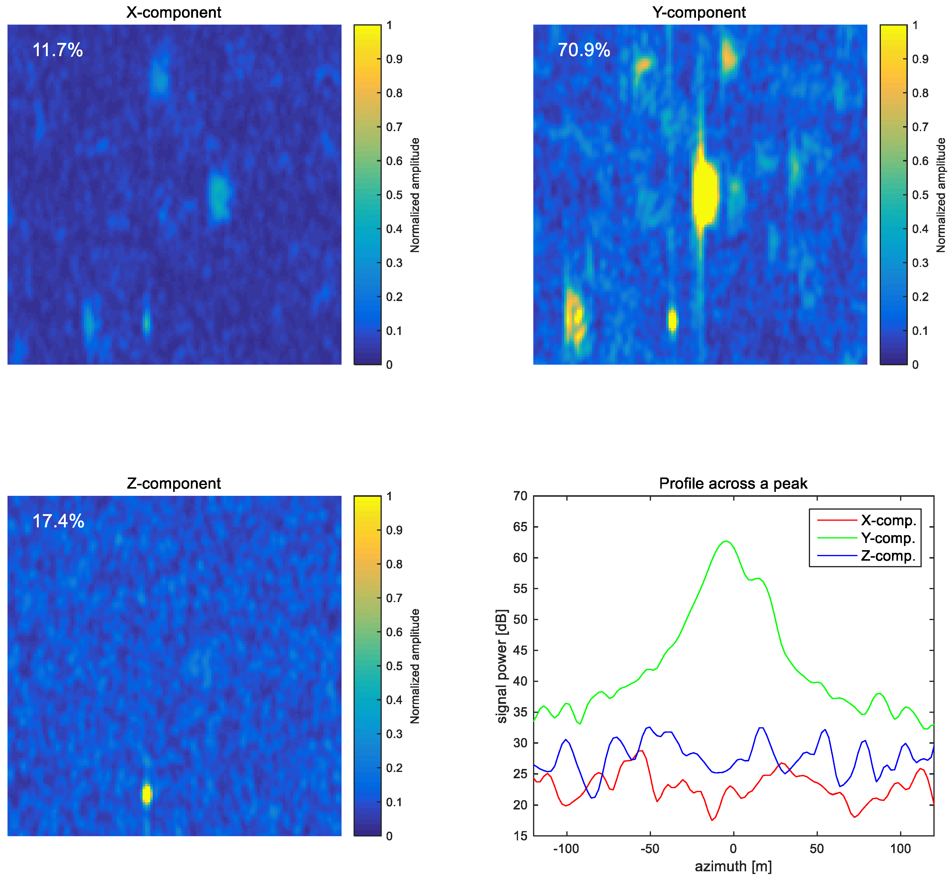
2.1. Characteristics of Azimuth Ambiguity and Multi-Look Processing

SAR azimuth ambiguities, or ghosts, have unique spectral features that distinguish them from true ground targets, such as small ships. Although both vessels and azimuth ambiguities commonly have strong signal strengths and are rendered by bright structures in images or time domains, the Doppler spectra of the two features are quite different. Typical Doppler spectra of a ship (blue line in Figure 1a) and a ghost (red line in Figure 1a) taken from TSX SLC data were used in this study. A typical Doppler spectrum from a true ground target is displayed with a blue line in Figure 1, showing characteristics of a symmetric center at a near-zero frequency and a broadband spectrum extending over the entire Doppler frequency, ranging from −PRF/2 to +PRF/2 (where PRF stands for pulse repetition frequency). Note that the Doppler spectrum of the ship does not extend to ±PRF/2, because the Doppler spectrum in SLC is intentionally limited to the total processed azimuth bandwidth shown in Table 1 by a SAR processor before delivering SLC data to users.
The Doppler frequency of a ground target displaced by an azimuth angle of Ψ from the antenna boresight is given by
f a = 2 V λ sin Ψ 2 V λ Ψ ,
where V is the antenna velocity and λ is the wavelength. If the Doppler frequency of the target is equal to a multiple of PRF, i.e., f a = m PRF , where m is the integer, then the target is aliased and imaged at the antenna boresight. As a consequence, if a target located at an azimuth angle satisfies the relation
Ψ λ 2 V m PRF ,
where m is an integer, which will be aliased to create ghost images and overlaid with true ground targets at the antenna boresight [7,17]. The contributions of aliased targets to the received signals are usually small if the two-way azimuth antenna beam pattern at angle Ψ is small compared with the beam center. If the area at the beam center has a low backscattering coefficient while the power of the antenna beam pattern at angle Ψ is relatively large, for instance, near coastal waters, the azimuth ambiguities become serious. Thus, the azimuth antenna beam pattern and selection of PRF are critical to the formation of the azimuth-ambiguity-to-signal ratio (AASR). In fact, most SAR systems are sophisticatedly designed to minimize azimuth ambiguities with consideration of the antenna beam pattern and look direction, PRF, satellite orbit, and attitude. Nevertheless, it is difficult to completely remove ghosts from SAR SLC images due to the nature of the antenna beam pattern and SAR systems.
Some distinctive features of the Doppler spectrum of the azimuth ambiguity depicted by the red line in Figure 1 are as follows: First, the distribution of the Doppler spectrum of the ghost is asymmetric with a spectral maximum near the Nyquist frequency. Second, the signal powers of the azimuth ambiguity are concentrated around the peak so that the effective bandwidth is much narrower than that of the ship. One of the most popular approaches to reducing ghosts in SAR images is to filter azimuth ambiguities, for instance, through an adaptive-filtering approach at each point [4] or with the Wiener-filter-based line-by-line processing approach [19]. The filtering approach is usually effective for suppressing azimuth ambiguities. It principally suppresses high-frequency components containing azimuth ambiguities; however, it unwantedly suppresses signal powers of fast-cruising vessels that are also characterized by a high-frequency Doppler centroid. Therefore, it is necessary to develop an approach that preserves ground targets with all plausible velocities while selectively removing ghosts. Here, we propose a simple but effective approach that uses axis rotation to separate true ground targets from ghosts and then effectively averages out the spectral powers of azimuth ambiguities while preserving the spectral powers of true ground targets.
Based upon the spectral characteristics of the ship and azimuth ambiguity or ghost shown in the SLC image, it was possible to design a SAR multi-look filter, as shown in Figure 1b. The three sub-apertures, shown in Figure 1b with green, blue, and red lines, will produce three sub-aperture images, also known as multi-look images, with a reduced spatial resolution but containing different signal powers. The three sub-apertures have a common bandwidth of one-third of the PRF. The centered frequencies of the green (sub-aperture for negative high frequencies), blue (sub-aperture for low frequencies), and red (sub-aperture for positive high frequencies) lines are at −PRF/3, 0, and +PRF/3, respectively. Considering the spectral characteristics of the ship and sub-apertures, all three multi-look images will maintain the signal powers of the ship, although the total signal power of the target in each sub-aperture will differ slightly according to the spectral pattern. On the contrary, the concentration of signal powers of the ghost in different multi-look images will largely vary between sub-apertures, for instance, they will be dominant in the negative high-frequency component but almost negligible in the positive high-frequency component.

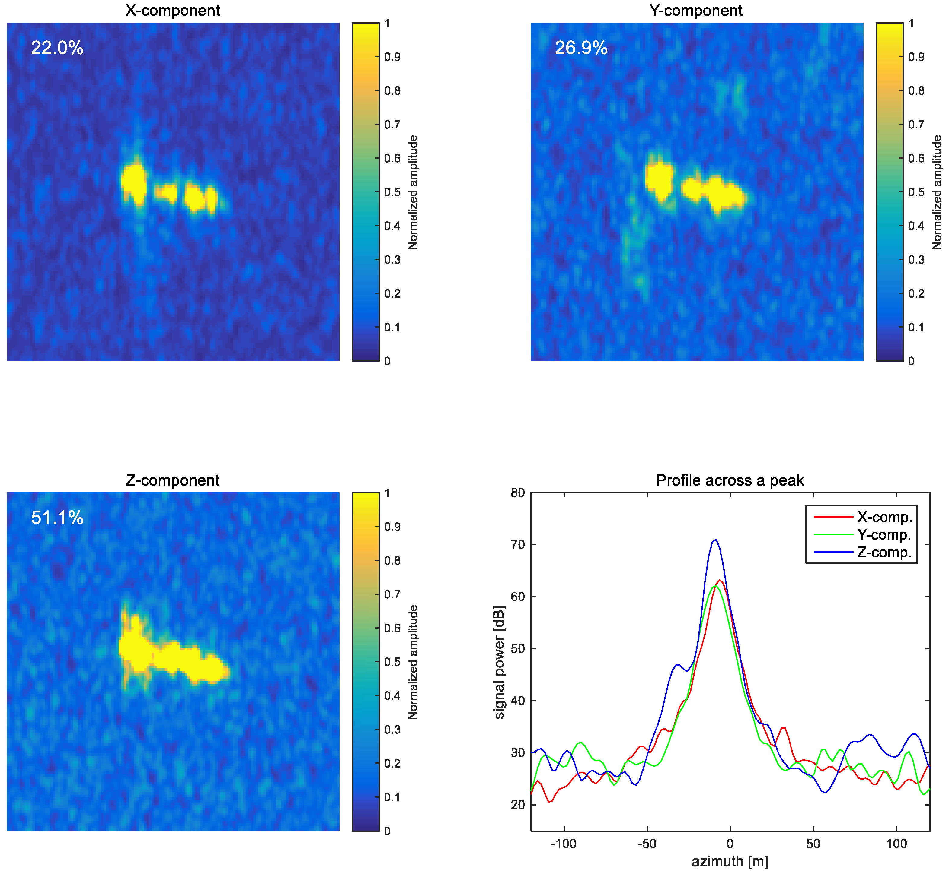
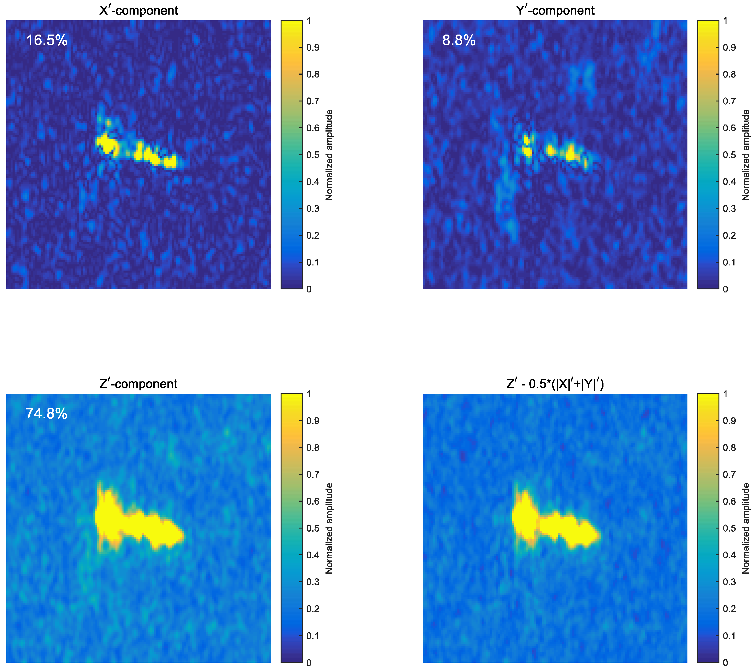
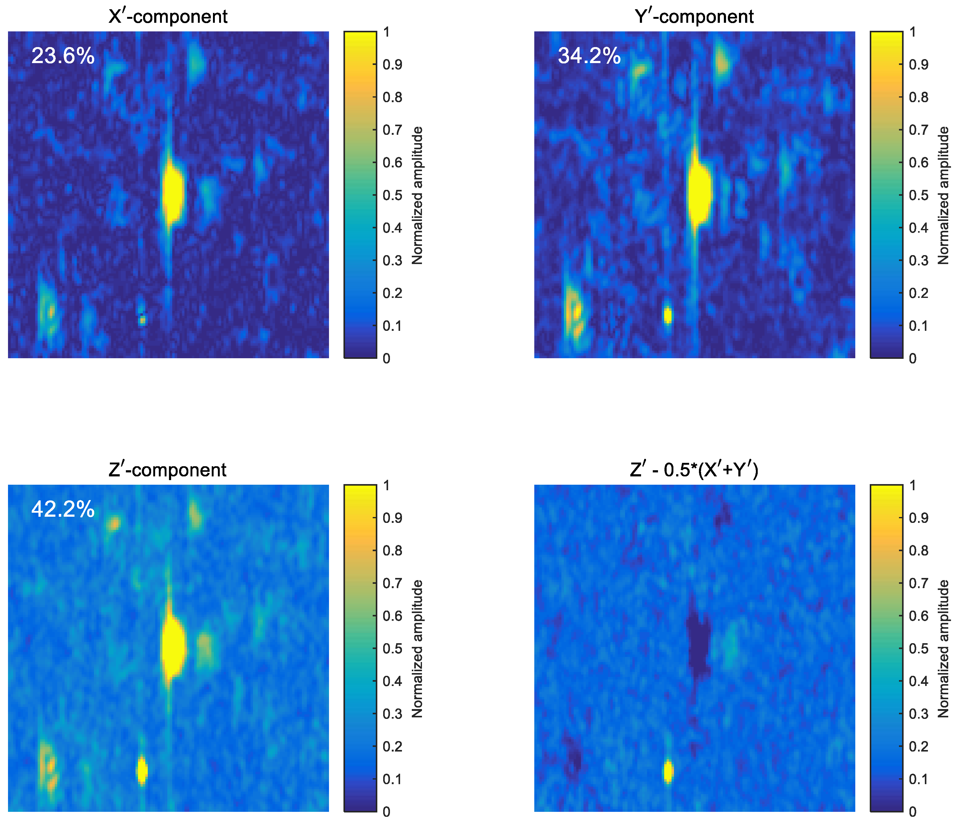
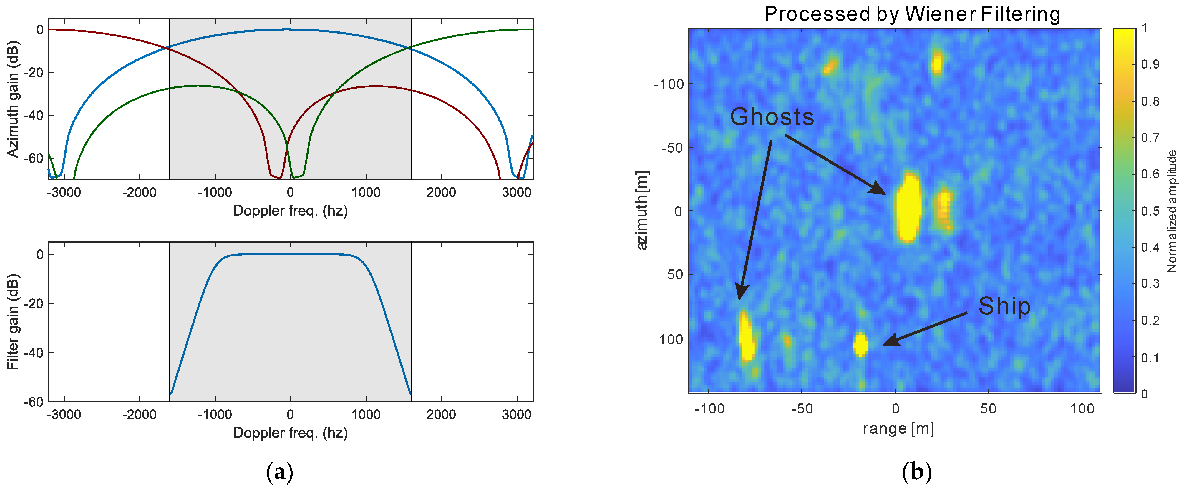
2.2. Core Idea and Method

As discussed in the previous sub-section, the patterns of the spectral distribution of true vessels and ghosts are distinctively different: vessels have a broadband Doppler spectrum while ghosts have a narrow, concentrated band. The core idea of this study is to project three multi-look (or sub-aperture) images onto a new coordinate system in which the spectral powers of true targets are concentrated at a single component, while those of ghosts are evenly dispersed over three different components. Projection to eigenvectors or principal component analysis (PCA) may be potential candidates for this purpose [5,24]. A method utilizing eigenvalues and eigenvectors, however, requires the estimation of eigenvectors for individual targets. Here, the proposed method is not designed to produce a perfectly reconstructed image for each individual target, but rather, for quick and effective generation of an image for an intermediate stage of target detection in coastal waters. From this, the detection of true vessels and other objects can be carried out. For this purpose, we propose a method that exploits a simple and target-independent axis rotation instead of using computationally inefficient individual target filtering or eigenvector analysis.
A rotation matrix can be obtained by matrix multiplication of the two basic rotation matrices rotating vectors by angles ψ and θ , such as
R = cos ψ sin ψ 0 sin ψ cos ψ 0 0 0 1 cos θ 0 sin θ 0 1 0 sin θ 0 cos θ = 0.5 0.7071 0.5 0.5 + 0.7071 0.5 0.7071 0 + 0.7071 ,
where ψ = 45 ° and θ = 45 ° are rotating angles about the z- and y-axes, respectively. Since the rotation matrix R is an orthogonal matrix, it satisfies the relationship given by
R 1 = R T ,
which means an inverse matrix or reverse rotation is obtained by the transpose of the rotation matrix.
The following simple rotation method is useful for the reduction of azimuth ambiguity.
X Y Z = R T X Y Z .
Matrix multiplication of the rotation matrix to (X, Y, Z) results in projection to a new coordinate (X′, Y′, Z′) in which the Z′-axis aligns with the vector 1 , 1 , 2 . Rotation of the vector 1 , 1 , 2 in (X, Y, Z) results in 0 , 0 , 2 in the rotated space, which implies that all signal powers are concentrated at a single component: the Z′-axis. On the contrary, the vector 0 , 2 , 0 in the (X, Y, Z) space is projected to a vector of 1 , 2 , 1 through the rotation. This means that rotation of a vector concentrated at a single X- or Y-axis through Equation (5) results in the dispersion of energy to three different components. For this rotation, the positive high-frequency band (red sub-aperture in Figure 1b) and negative high-frequency band (green sub-aperture in Figure 1b) are assigned to the X- and Y-components, respectively, and the low-frequency band (blue sub-aperture in Figure 1b) is assigned to the Z-component.
Once the axis-rotated components (X′, Y′, Z′) have been obtained by Equation (5), the signal powers of ghosts can be significantly suppressed by a simple operation:
D = Z w · X + Y ,
where w is a weight, which was assigned a value of 0.5 in this study. The weight of 0.5 means a subtraction of a simple mean of X′- and Y′-component from Z′-component, provided that the AAP is symmetric with a zero Doppler centroid. Different weights can be used according to the AAP and spectral characteristics of azimuth ambiguities in a given SAR image. An optimum weight for the test data used in this study will be discussed in the Section 3.4. The sum and difference operation of Equation (6) will completely remove ghosts if ghost signals are evenly distributed among the X′-, Y′- and Z′-axes, while all signal powers of a ship will be solely concentrated in the Z′-axis with the X′- and Y′-components having values of 0. Although this assumption may not be satisfied for all cases, Equation (6) efficiently and significantly suppresses ghosts rendered in most SAR images. Then, the final output of the ghost-removed image can be obtained by
D g r = 1 2 D i f   D 0 0 i f   D < 0 .
The main advantages of the proposed method are its high performance and computational simplicity. It is not necessary to estimate spectral characteristics of ghosts individually or on a line-by-line basis. The rotation completed with Equation (5) is also straightforward and computationally efficient and is followed by a simple summation and subtraction using Equations (6) and (7). For an image with a size of N pixels, the processing of Equations (5)–(7) only requires a total computational cost of O(3 × 3N + 2N). Thus, it is faster than any procedure comparable to a convolution with a sliding window of 4 × 3 samples. Therefore, this method is a very efficient way to carry out simple computations over whole areas of interest. This simple procedure provides images with competitive quality that can be used for the detection of vessels or other sea surface objects in subsequent tasks. The performance details of the proposed method are discussed in the next section.

3. Application Results and Discussion

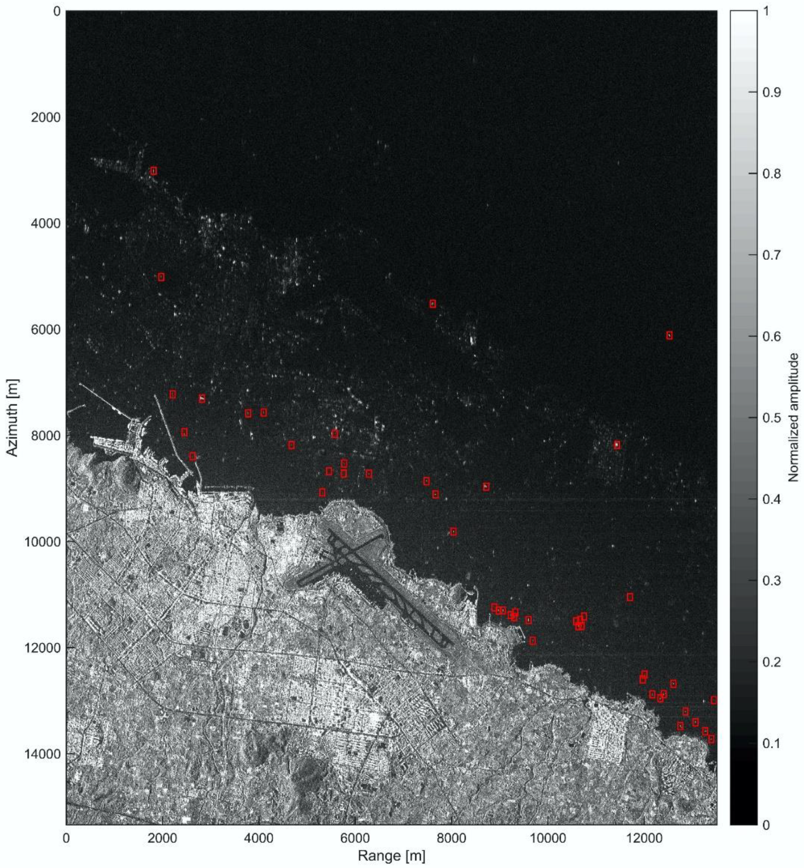
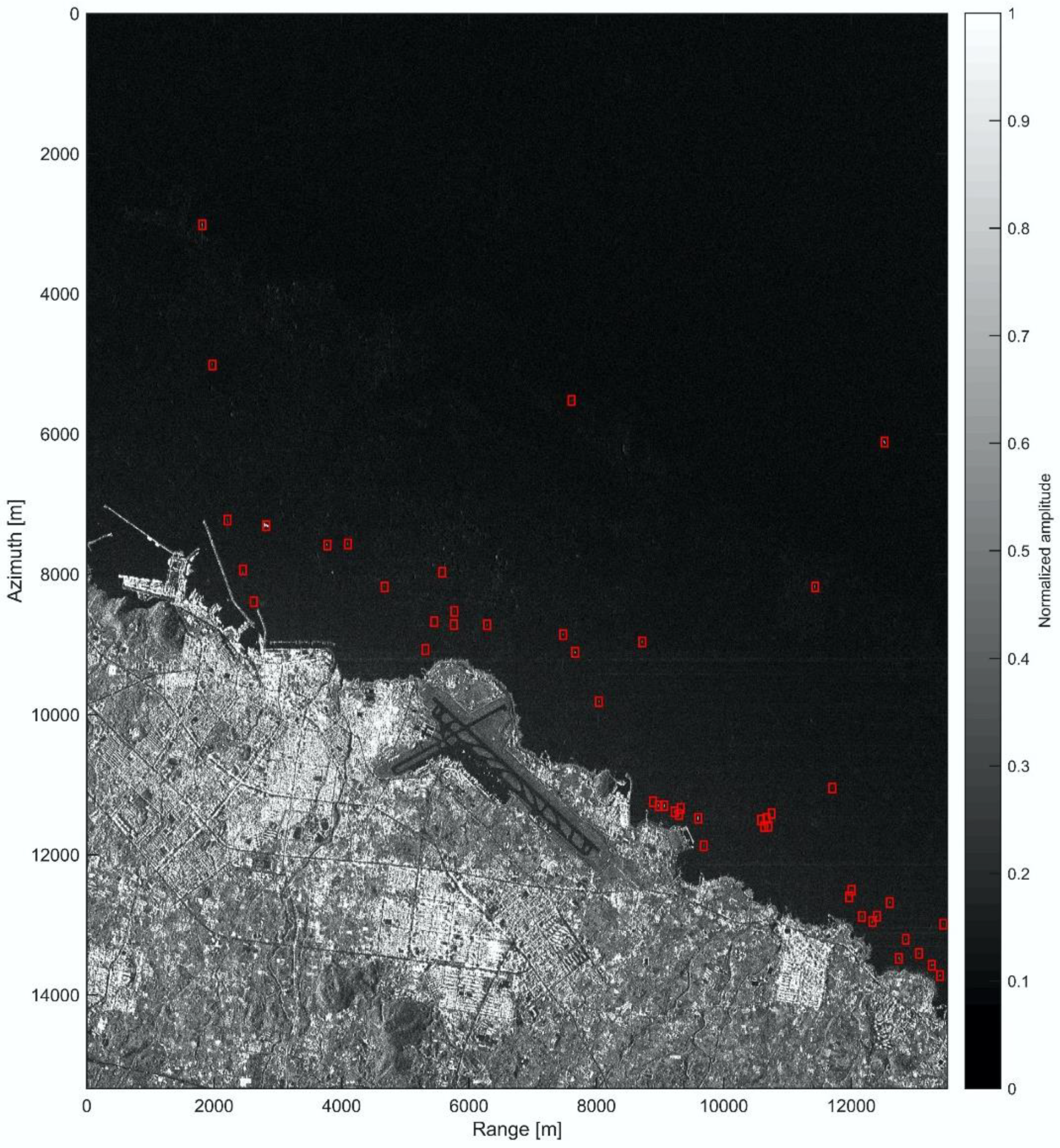
3.1. SAR Data in Coastal Regions

SAR test data were acquired by the TSX descending mode with an incidence angle of 53.8 degrees at the scene center, as shown in Figure 2. The system parameters of the data used in this study are summarized in Table 1. The SAR image was obtained for an experiment on the detection of small vessels in coastal waters. For this experiment, vessels in coastal waters at the moment of SAR observation were traced by the automatic identification system (AIS). Figure 2 displays the amplitude of the SAR single-look complex (SLC) signal normalized by the value pertaining to 96% of the statistical distribution of the amplitude, and the locations of vessels are denoted by red squares.
The SAR image of the near-coastal sea surface was severely overlaid with azimuth ambiguities (or ghosts), as shown in Figure 2. The azimuth time displacement of a ghost from the true target can be approximately calculated by PRF Time, which is defined as the ratio of PRF to the Doppler rate:
P R F   T i m e = ± PRF K a ,
where K a is the Doppler rate [17,25]. The PRF Time value of the TSX data used in this study was 0.7513 s, as shown in Table 1, which corresponds to about 5287 m in the image. Therefore, true features located in coastal waters within about 5.3 km from the coastline were mixed with azimuth ambiguities from strong land structures. Consequently, it was very difficult to detect or discriminate ghost targets from true vessels or rocks exposed on the sea surface without efficient reduction of azimuth ambiguities, as shown in Figure 2.

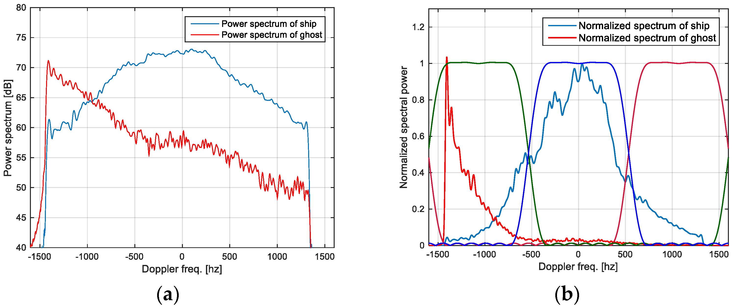
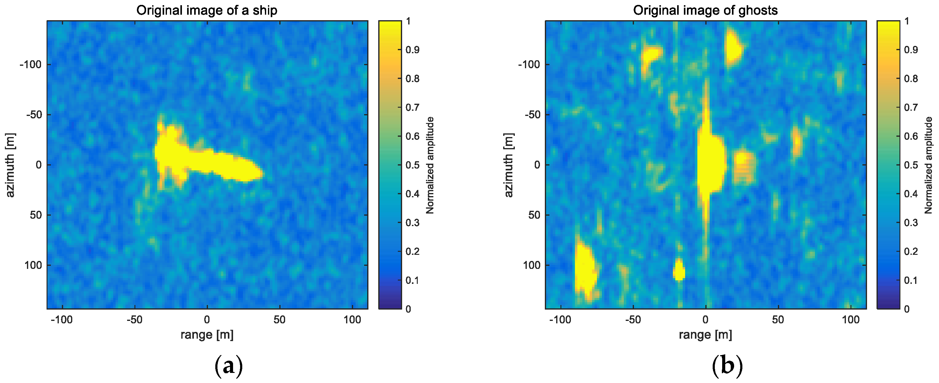
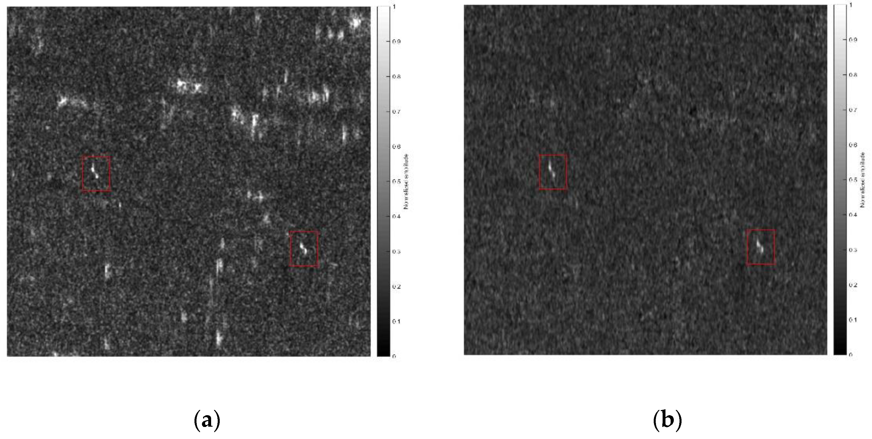
3.2. Comparison between Vessels and Ghosts

Two sub-areas with a window of 129 by 129 samples were first taken around a typical ship (Figure 3a) and ghosts (Figure 3b). Since the signal power of ghosts is very high compared with that of typical vessels, as shown in Figure 3, it was almost impossible to discriminate true vessels in these coastal waters from ghosts without the suppression of ghost targets.
Three different multi-look components were computed through band-pass filtering. Figure 4 displays the three sub-aperture components of the ship. The low-frequency component assigned to the Z-axis naturally shows the largest power concentration, accounting for 51.1% of the total signal power. This can be explained by two facts: First, the Doppler spectrum follows a sinc squared function, as shown in Figure 1, due to its antenna beam pattern and azimuth window applied by the SAR processor [25]. Second, the total azimuth bandwidth maintained in the SLC image is only 86.9% of the PRF, as shown in Table 1, because about 14% of high-frequency components were intentionally erased by the SAR processor to reduce azimuth ambiguities. Since image formation from raw SAR signals through a SAR processor is normally carried out by a data provider, general users are not able to restore the deleted high-frequency components. Thus, the signal strength of low-frequency components or central frequency parts is usually stronger than that of high-frequency components. Nevertheless, high-frequency components of the true ship also contribute to about half of the total strength of the signal, as shown in Figure 4. The positive high-frequency component (upper left in Figure 4) and negative high-frequency component (upper right in Figure 4) account for 22.0% and 26.9% of the signal, respectively. Azimuth profiles of the three components across the signal peak are shown in the bottom right plot in Figure 4. While the peak signal power of the low-frequency component (or the Z-component), shown by the blue line, was the highest, the negative high-frequency component (or the X-component), shown in red, and the positive high-frequency component (or Y-component), shown in green, also showed similar patterns of power distribution to the Z-component with comparable peak powers of no less than 5 dB.
The same procedure was applied to the sub-area containing ghosts in Figure 3 to obtain the three multi-look components shown in Figure 5. Although the original images of ships and ghosts shown in Figure 3 look very similar to each other, the characteristics of the multi-look components shown in Figure 4 and Figure 5 are distinctively different. The signal powers concentrated in the positive high-frequency component assigned to the X-axis (upper left in Figure 5) and the low Doppler frequency component assigned to the Z-axis (bottom left in Figure 5) were insignificant and accounted for only 11.7% and 17.4% of the total signal power, respectively. A large portion of the ambiguity signal (70.9%) was found to be concentrated at the single dominant Y-component. Azimuth profiles across a peak (bottom right in Figure 5) also depicted this feature such that the peak power of the Y-component was found to be distinctively larger than those of the X- and Z-components by about 35 dB.
From the three multi-look components of the original images presented in Figure 4 and Figure 5, a new output projected to the rotated axis (X′, Y′, Z′) was obtained by applying the rotation matrix represented by Equation (5). The axis rotation resulted in three new components of the ship and ghosts, as summarized in Figure 6 and Figure 7, respectively. In Figure 6, the three components projected to the rotated axes of X′, Y′, and Z′ show a concentration of signal powers on the Z′-axis, as expected. The Z′-component accounts for 74.8% of the total signal power, while the X′- and Y′-components account for only 16.5% and 8.8%, respectively.
The simple arithmetic operation presented in Equation (6) produced the output displayed at the bottom right of Figure 6. The output preserved the original features of the ship well. On the contrary, signal powers of ghosts were dispersed over three new axes after axis rotation by Equation (5), as shown in Figure 7. While the signal powers of ghosts were originally mainly concentrated at the Y-axis, as shown in Figure 5, they became almost evenly distributed among the X′-axis (upper left), Y′-axis (upper right), and Z′-component (bottom left) with portions of the total signal power of 23.6%, 34.2%, and 42.2%, respectively. Then, a simple processing step is done using Equations (5)–(7) effectively reduced the ghosts while preserving true ground targets, as shown in the bottom right of Figure 7. A comparison between the result for ghosts, shown in Figure 7, and that for a ship, shown in Figure 6, demonstrates the effectiveness of the proposed method for reducing ghosts or azimuth ambiguities while preserving true ground targets.

3.3. Results of the Application for the Whole Area
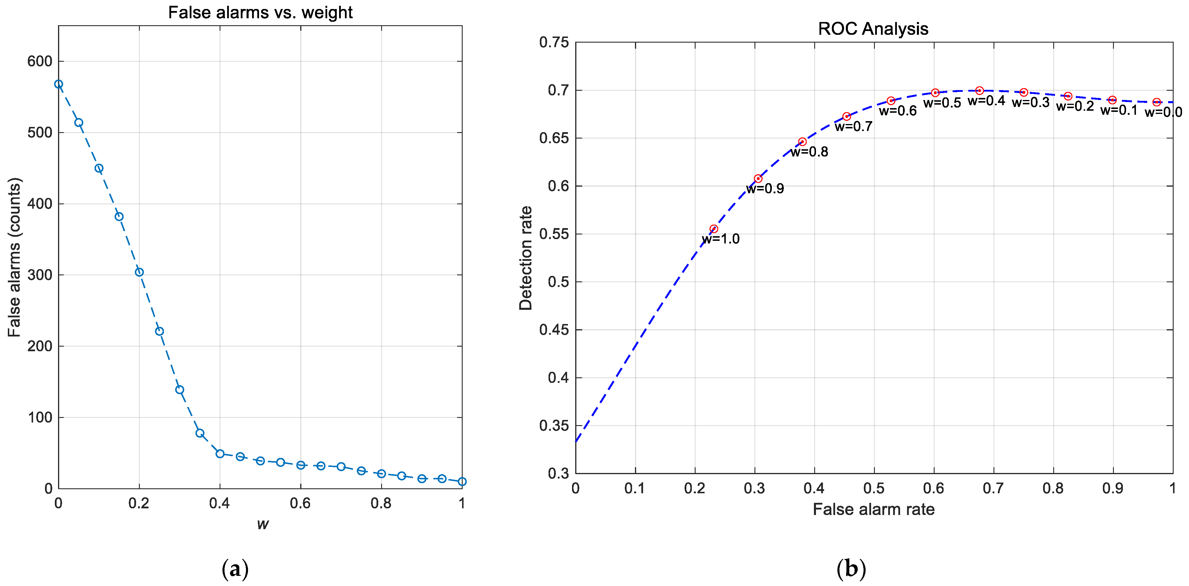
As the effectiveness of the proposed method was proven using a selected ship and ghost, we also applied the method to the scene shown in Figure 2. Figure 8 displays the results of ghost reduction processing overlaid with locations of vessels tracked by the AIS system. Compared with the original TSX image presented in Figure 2, ghost targets scattered within 5.3 km of the coastline were efficiently and effectively suppressed. The resulting image could be used to detect and analyze vessels and rocks exposed above the water surface.
To investigate the processing results in more detail, a pair of enlarged images of an area of 2 by 2 km is shown in Figure 9. Figure 9a,b displays the original TSX SLC image and the processing output overlaid with locations of vessels tracked by the AIS system. Both images were normalized by a common value of 96% of the statistical distribution of the amplitude for comparison. It was almost impossible to detect and discriminate true vessels by visual inspection or automatic detection from the original TSX SLC image presented in Figure 9a because true vessels were severely mixed with bright ghosts. A number of vessels in this area were less than 60 m in length. The government and other groups are interested in small-sized vessels as these are involved in illegal activities more frequently than large ships. It is, however, very difficult for small vessels with lengths of less than a few tens of meters to be visually or automatically detected from SAR images. Ghost targets rendered by azimuth ambiguities make it much harder to detect ships in the water near the coast, as shown in Figure 2 and Figure 9a. In the processed image Figure 9b, vessels are now clearly detectable with a high level of confidence in contrast with Figure 9a. The bright ghosts in Figure 9a were effectively suppressed by the proposed method, while vessels were well preserved in terms of signal strength and shape, regardless of their size, as in Figure 9b. Two small ships were successfully detected from Figure 9b. The resulting images shown in Figure 8 and Figure 9b demonstrate that the proposed method significantly improves SAR detectability for targets near the coast, including small vessels and exposed bottom rocks.
For evaluation of performance of the proposed method and determination of an optimum weight of w in Equation (6), a Receiver Operating Characteristic (ROC) analysis was carried out. The ROC curve has long been used in signal detection theory to depict the tradeoff between hit rates and false alarm rates of classifiers [26,27,28]. At the time of the TSX data acquisition, there were a total of 51 ships and boats within the scene of Figure 8 according to AIS records. The constant false alarm (CFAR) method is popularly for detection of vessels in the SAR image [29], and we adopted a general CFAR for ship detection in this study. It is often difficult to detect small boats less than several meters in length regardless of ghosts. Figure 10a shows the total number of false alarms varying with the weight w in Equation (6). The weight w = 0 produces an image before ghost removal, from which a total of 568 false alarms was detected. The total number of false alarms decreases up to w = 0.4 with a steep slope as in Figure 10a, then the trend of decrease changes to a gentle slope. The total number of false alarms was significantly reduced to 39 in the image of w = 0.5 from 568 before ghost removal, which is about 93% removal of false alarms. The false alarm removal rate is important because the main purpose of ghost suppression is to reduce the total number of unwanted detections. Although the false alarm rate continuously decreases as the value of weight increases, the w higher than 0.5 also reduces the detection rate as in the ROC curve in Figure 10b. The detection rate reaches the maximum at w = 0.5 with a false alarm rate of about 0.6. The maximum detection rate did not reach 1.0, but instead reached 0.7 because of undetected small boats. Thus, the weight of 0.5 is the optimum for this data. The area under the curve (AUC) is 0.62. The results demonstrate its capability to effectively suppress ghosts and validate the use of weight w = 0.5 in Equation (6) for this test data.
In summary, the proposed algorithm can be used to produce an intermediate output that may be used for the detection of ships or other targets in coastal waters.

3.4. Discussion

The effectiveness of the proposed method can be supported by comparison with results of the Wiener filtering. Figure 11 displays an example of azimuth ambiguity removal by applying the Wiener filter proposed by [17] to the same area of interest in Figure 7. The Wiener filter must be designed by considering the azimuth antenna pattern (AAP) of each individual dataset. Figure 11a shows the AAP and its first replicas responsible for aliasing of the TSX data used in this study (above), and the Wiener filter gain derived from the AAP and its left and right replicas (below). Ghosts in the resulting image of Wiener filtering Figure 11b are not completely removed. The Wiener approach usually requires some additional steps at the cost of increasing computational burden such as [17,19] to effectively suppress ambiguities. Compared (b) with the resulting image in Figure 7 (bottom right), the proposed method does very effectively suppress ghosts while preserving vessels. This example demonstrates that the proposed approach is useful for pre-processing of SAR images to detect vessels in coastal water.
The proposed method has various advantages in terms of performance and computational simplicity for the detection of vessels from SAR images in coastal water. However, the proposed method has some limitations regarding its application. Although the proposed method effectively reduces the azimuth ambiguities in the final output, some persistent ghosts still exist, as shown in Figure 9b. Additional procedures must be used to determine whether detected bright features represent a true ground target or ghost by examining residual Doppler frequencies. The Doppler spectrum of these persistent ghosts is different from that shown in Figure 1 and is characterized by a slight broadband at positive high frequencies with a smaller signal power. This implies that the performance of the proposed method depends on the degree of concentration of the spectral power of azimuth ambiguities. As it concentrates at a narrow frequency band close to the Nyquist frequency (or one-half of positive or negative PRF), the performance of the method significantly improves. Otherwise, the band-pass filter adopted in this study to generate three multi-look images should be modified to accommodate different spectral characteristics of the SAR dataset being used. In addition, the optimal rotation angle about the y-axis may need to be reviewed according to the ratio of the signal power of the high-frequency band to the low-frequency band. The core idea of the approach is to make a broadband spectrum of the true target into a single component by axis rotation. The TSX data used in this study has the AAP as shown in Figure 11a (above), and the ratio of the antenna gain sum of the central aperture (blue in Figure 1b) to the gain summation mean of the side apertures (green and red in Figure 1b) is 1.41 which approximates to 2 . The rotation by Equation (3) projects 1 , 1 , 2 in (X, Y, Z) to 0 , 0 , 2 in the rotated space (X′, Y′, Z′), and it theoretically works well for the TSX data used in this study. The gain ratio depends on the AAP of each SAR system and the Doppler centroid of individual SAR image. It would be necessary to determine the optimum rotation angle for each SAR systems or images. Rotation aligning to eigenvectors would be an alternative approach, but it is not as effective as Equation (3) in the author’s experience. Eigenvectors of a small area of interest would be meaningful, but eigenvectors estimated over the whole scene (excluding landmass) are corrupted by ambiguities and various sea surface features including currents and waves. The axis rotation by 45° for both ψ and θ as in Equation (3) also works well for data obtained by other SAR systems, for instance KOMSAT-5 X-band SAR. It is necessary to carry out further study on determination of the optimum rotation angle for various SAR systems in the future.
The Doppler centroid of the SAR SLC image must also be checked before applying the proposed method. Some SAR systems provide a zero-Doppler SLC image in which the Doppler centroid has a near-zero frequency. These require precise maneuvering of the satellite attitude and antenna beam [8,30], but many current SAR systems have a limited capability for satisfying these requirements. In such cases, the band-pass filter should be shifted in frequency according to the given Doppler centroid of the SAR SLC data used.
Once the three multi-look images are projected to the new coordinate (X′, Y′, Z′) by the rotation matrix, Equation (5), a simple arithmetic computation in Equations (6) and (7) is applied to obtain the ghost suppressed output. This is a calculation of weighted sum and difference using a weight of 0.5 for both the X′- and Y′-components. This worked very well for the test data used in this study. Although this method is simple and straightforward, the optimal weight differs according to the spectral characteristics of the input data.

4. Conclusions

A new approach for the suppression of azimuth ambiguities or ghosts in high-resolution SAR SLC images using simple axis rotation was introduced and discussed in this paper. While Wiener or other types of filtering of ghosts are effective for azimuth ambiguity reduction, these methods carry the risk of unintentionally removing fast cruising ships. Instead of directly filtering ghost signals, the method exploits different patterns of signal power distribution of vessels and ghosts in three sub-aperture images. A simple axis rotation projects the dispersed signal powers of the vessels onto a single axis while making those of ghosts disperse among three axes. In the new rotated coordinate, the ghosts can easily be suppressed by a simple arithmetic operation while effectively maintaining the signals of true targets. The results obtained by applying the method to TSX SLC data demonstrated that the method can effectively suppress ghosts while preserving small and fast cruising ships in coastal waters. The capabilities of ship detection from the test image were significantly improved by reducing 93% of false alarms. The computational burden is low, so it can be used to efficiently provide images for use in coastal ship detection.
Although the results obtained by applying the proposed method to the test data demonstrated its capability of ghost suppression, the proposed method has some limitations regarding its application. It requires investigation into the optimum rotation angles in Equation (3) according to characteristics of various SAR systems and ghosts in the future. In addition, it is also necessary to further examine the methods of summation to replace Equation (6). Although this approach is simple and straightforward, the optimal weight might differ according to the spectral characteristics of the input data.
In the future study, it would be valuable to investigate the use of optical images combined with SAR images in this region through information fusion. For instance, the Visible Infrared Imaging Radiometer (VIIRS) day/night band (DNB) satellite images are proven to be a useful tool to monitor ships at nighttime with a limited spatial resolution [31,32]. A total number of ships and boats involved in illegal activities usually increases during the night. Thus, the combined use of SAR and VIIRS DNB as well as high resolution optic images would improve the capability of monitoring vessels from space in coastal waters.

Author Contributions

Conceptualization, J.-S.W.; methodology, J.-S.W. and J.H.C.; validation, J.H.C.; formal analysis, J.H.C. and J.-S.W.; investigation, J.H.C. and J.-S.W.; data curation, J.-S.W.; writing—original draft preparation, J.-S.W.; writing—review and editing, J.-S.W. and J.H.C.; visualization, J.H.C. and J.-S.W.; project administration, J.-S.W.; funding acquisition, J.-S.W. All authors have read and agreed to the published version of the manuscript.

Funding

This study was funded by the Korea Ministry of Environment (MOE) under the Service Program for Demand-Responsive Water Supply (2019002650004) and partially supported by the Korea Institute of Marine Science and Technology Promotion funded by the Korea Coast Guard for the “Development of satellite based system on monitoring and predicting ship distribution in the contiguous zone” projects for field data acquisition.

Institutional Review Board Statement

Not applicable.

Informed Consent Statement

Informed consent was obtained from all subjects involved in the study.

Acknowledgments

The authors sincerely appreciate all scientists and graduate students involved in the field experiments.

Conflicts of Interest

The authors declare no conflict of interest.

References

  1. Brusch, S.; Lehner, S.; Fritz, T.; Soccorsi, M.; Soloviev, A.; van Schie, B. Ship Surveillance With TerraSAR-X. IEEE Trans. Geosci. Remote Sens. 2011, 49, 1092–1103. [Google Scholar] [CrossRef]
  2. Iervolino, P.; Guida, R.; Whittaker, P. A novel ship-detection technique for Sentinel-1 SAR data. In Proceedings of the 2015 IEEE 5th Asia-Pacific Conference on Synthetic Aperture Radar, APSAR 2015, Singapore, 1–4 September 2015; pp. 797–801. [Google Scholar]
  3. Lee, J.S.; Jurkevich, I. Coastline Detection and Tracing in SAR Images. IEEE Trans. Geosci. Remote Sens. 1990, 28, 662–668. [Google Scholar] [CrossRef] [Green Version]
  4. Back, M.; Kim, D.; Kim, S.W.; Won, J.S. Two-Dimensional Ship Velocity Estimation Based on KOMPSAT-5 Synthetic Aperture Radar Data. Remote Sens. 2019, 11, 1474. [Google Scholar] [CrossRef] [Green Version]
  5. Yi, N.; He, Y.J.; Liu, B.C. Improved Method to Suppress Azimuth Ambiguity for Current Velocity Measurement in Coastal Waters Based on ATI-SAR Systems. Remote Sens. 2020, 12, 3288. [Google Scholar] [CrossRef]
  6. Santamaria, C.; Greidanus, H. Ambiguity discrimination for ship detection using Sentinel-1 repeat acquisition operations. In Proceedings of the International Geoscience and Remote Sensing Symposium (IGARSS), Milan, Italy, 26–31 July 2015; pp. 2477–2480. [Google Scholar]
  7. Li, F.K.; Johnson, W.T.K. Ambiguities in Spaceborne Synthetic Aperture Radar Systems. IEEE Trans. Aerosp. Electron. Syst. 1983, 19, 389–397. [Google Scholar] [CrossRef]
  8. Raney, R.K. Doppler Properties of Radars in Circular Orbits. Int. J. Remote Sens. 1986, 7, 1153–1162. [Google Scholar] [CrossRef]
  9. Rolt, K.D.; Schmidt, H. Azimuthal Ambiguities in Synthetic Aperture Sonar and Synthetic Aperture Radar Imagery. IEEE J. Ocean. Eng. 1992, 17, 73–79. [Google Scholar] [CrossRef]
  10. Freeman, A.; Johnson, W.T.K.; Huneycutt, B.; Jordan, R.; Hensley, S.; Siqueira, P.; Curlander, J. The “myth” of the minimum SAR antenna area constraint. IEEE Trans. Geosci. Remote Sens. 2000, 38, 320–324. [Google Scholar] [CrossRef] [Green Version]
  11. Gebert, N.; Krieger, G.; Moreira, A. Digital Beamforming on Receive: Techniques and Optimization Strategies for High-Resolution Wide-Swath SAR Imaging. IEEE Trans. Aerosp. Electron. Syst. 2009, 45, 564–592. [Google Scholar] [CrossRef] [Green Version]
  12. Kim, J.H.; Younis, M.; Prats-Iraola, P.; Gabele, M.; Krieger, G. First Spaceborne Demonstration of Digital Beamforming for Azimuth Ambiguity Suppression. IEEE Trans. Geosci. Remote Sens. 2013, 51, 579–590. [Google Scholar] [CrossRef] [Green Version]
  13. Villano, M.; Krieger, G.; Jäger, M.; Moreira, A. Staggered SAR: Performance Analysis and Experiments with Real Data. IEEE Trans. Geosci. Remote Sens. 2017, 55, 6617–6638. [Google Scholar] [CrossRef]
  14. Villano, M.; Krieger, G.; Moreira, A. New Insights Into Ambiguities in Quad-Pol SAR. IEEE Trans. Geosci. Remote Sens. 2017, 55, 3287–3308. [Google Scholar] [CrossRef]
  15. Younis, M.; Fischer, C.; Wiesbeck, W. Digital beamforming in SAR systems. IEEE Trans. Geosci. Remote Sens. 2003, 41, 1735–1739. [Google Scholar] [CrossRef]
  16. Moreira, A. Suppressing the Azimuth Ambiguities in Synthetic Aperture Radar Images. IEEE Trans. Geosci. Remote Sens. 1993, 31, 885–895. [Google Scholar] [CrossRef]
  17. Guarnieri, A.M. Adaptive removal of azimuth ambiguities in SAR images. IEEE Trans. Geosci. Remote Sens. 2005, 43, 625–633. [Google Scholar] [CrossRef]
  18. Villano, M.; Krieger, G. Spectral-Based Estimation of the Local Azimuth Ambiguity-to-Signal Ratio in SAR Images. IEEE Trans. Geosci. Remote Sens. 2014, 52, 2304–2313. [Google Scholar] [CrossRef]
  19. Martino, G.D.; Iodice, A.; Riccio, D.; Ruello, G. Filtering of Azimuth Ambiguity in Stripmap Synthetic Aperture Radar Images. IEEE J. Sel. Top. Appl. Earth Obs. Remote Sens. 2014, 7, 3967–3978. [Google Scholar] [CrossRef] [Green Version]
  20. Long, Y.J.; Zhao, F.J.; Zheng, M.J.; Jin, G.D.; Zhang, H. An Azimuth Ambiguity Suppression Method Based on Local Azimuth Ambiguity-to-Signal Ratio Estimation. IEEE Geosci. Remote Sens. Lett. 2020, 17, 2075–2079. [Google Scholar] [CrossRef]
  21. Meng, H.; Chong, J.S.; Wang, Y.H.; Li, Y.; Yan, Z.F. Local Azimuth Ambiguity-to-Signal Ratio Estimation Method Based on the Doppler Power Spectrum in SAR Images. Remote Sens. 2019, 11, 857. [Google Scholar] [CrossRef] [Green Version]
  22. Zeng, T.; Lu, Z.; Ding, Z.; Bian, M. SAR Doppler Ambiguity Resolver Based on Entropy Minimization. IEEE Trans. Geosci. Remote Sens. 2013, 51, 4405–4416. [Google Scholar] [CrossRef]
  23. Scheiber, R.; Jäger, M. Detection and mitigation of strong azimuth ambiguities in high resolution SAR images. In Proceedings of the European Conference on Synthetic Aperture Radar, EUSAR, Hamburg, Germany, 6–9 June 2016. [Google Scholar]
  24. Liu, B.C.; He, Y.J.; Li, Y.K.; Duan, H.Y.; Song, X. A New Azimuth Ambiguity Suppression Algorithm for Surface Current Measurement in Coastal Waters and Rivers With Along-track InSAR. IEEE Trans. Geosci. Remote Sens. 2019, 57, 3148–3165. [Google Scholar] [CrossRef]
  25. Cumming, I.G.; Wong, F.H. Digital Processing of Synthetic Aperture Radar Data: Algorithms and Implementation; Artech House: Boston, MA, USA, 2005; p. 625. [Google Scholar]
  26. Begueria, S. Validation and evaluation of predictive models in hazard assessment and risk management. Nat. Hazards 2006, 37, 315–329. [Google Scholar] [CrossRef] [Green Version]
  27. Zou, K.H.; O’Malley, A.J.; Mauri, L. Receiver-operating characteristic analysis for evaluating diagnostic tests and predictive models. Circulation 2007, 115, 654–657. [Google Scholar] [CrossRef] [PubMed] [Green Version]
  28. Fawcett, T. An introduction to ROC analysis. Pattern Recogn. Lett. 2006, 27, 861–874. [Google Scholar] [CrossRef]
  29. Pappas, O.; Achim, A.; Bull, D. Superpixel-Level CFAR Detectors for Ship Detection in SAR Imagery. IEEE Geosci. Remote Sens. Lett. 2018, 15, 1397–1401. [Google Scholar] [CrossRef] [Green Version]
  30. Fiedler, H.; Boerner, E.; Mittermayer, J.; Krieger, G. Total zero Doppler steering—A new method for minimizing the Doppler centroid. IEEE Geosci. Remote Sens. Lett. 2005, 2, 141–145. [Google Scholar] [CrossRef]
  31. Cozzolino, E.; Lasta, C.A. Use of VIIRS DNB satellite images to detect jigger ships involved in the Illex argentinus fishery. Remote Sens. Appl. Soc. Environ. 2016, 4, 167–178. [Google Scholar] [CrossRef]
  32. Kim, E.; Kim, S.W.; Jung, H.C.; Ryu, J.H. Moon Phase based Threshold Determination for VIIRS Boat Detection. Korean J. Remote Sens. 2021, 37, 69–84. [Google Scholar] [CrossRef]
Figure 1. Doppler spectra of a true ship and azimuth ambiguity (or ghost). (a) Power spectra presented in decibel units. (b) Power spectra presented as normalized spectral power overlaid with three sub-apertures that were used for multi-look processing in this study. While the Doppler spectrum of the ship is spread over the entire spectral band, that of the azimuth ambiguity is characterized by a narrow bandwidth centred close to ±PRF/2.
Remotesensing 13 04865 g001
Figure 2. Test image of the northern coast of Jeju Island. The SAR data were acquired by the TerraSAR-X descending model with an incidence angle of 53.8 degrees at the scene centre. Red squares indicate the locations of vessel traced by the AIS system. True marine targets, such as vessels or bottom rocks, exposed above the water surface are severely mixed with ghosts (or azimuth ambiguities) in the coastal water, and consequently, it is very difficult to detect true coastal targets.
Remotesensing 13 04865 g002
Figure 3. Sub-sampled amplitude images of a typical (a) ship and (b) ghosts. The sample size of the two areas was 129 by 129 in terms of the range and azimuth, respectively. Both images were normalized by a common value pertaining to 96% of the statistical distribution of the amplitude over the whole area in Figure 2.
Remotesensing 13 04865 g003
Figure 4. Three different views computed from a typical ship with a window containing 129 by 129 sub-samples. The positive high Doppler frequency component was assigned to the X-axis (upper left), the negative high Doppler frequency component was assigned to the Y-axis (upper right), and the low Doppler frequency component was assigned to the Z-axis (bottom left). Azimuth profiles across a peak were also compared (bottom right), and the maximum peak powers of the X- and Y-components were no lower than 5 dB compared with the Z-component. The summed signal power of the Z-component accounted for 51.1% of the total signal power, and the X- and Y-components accounted for about 22.0% and 26.9%, respectively.
Remotesensing 13 04865 g004
Figure 5. Three different views computed from the sub-area containing ghosts in Figure 3b. The positive high-frequency component was assigned to the X-axis (upper left), the negative high-frequency component was assigned to the Y-axis (upper right), and the low Doppler frequency component was assigned to the Z-axis (bottom left). The summed signal powers of the X- and Z-components account only for 11.7% and 17.4% of the total signal power, respectively, while the signal power is concentrated on the single dominant Y-component, 70.9%. Azimuth profiles across the brightest peak were compared (bottom right), and the maximum peak powers of the X- and Z-components were found to be insignificant and lower than that of the Y-component by about 35 dB.
Remotesensing 13 04865 g005
Figure 6. Projection of multi-look components of the ship to new axes (X′, Y′, Z′) by the rotation matrix of Equation (5). Compared with the original (X, Y, Z) components shown in Figure 4, the signal power of the ship is now concentrated at the Z′-component (bottom left). While the projected signals at the X′-axis (upper left) and Y′-axis (upper right) account for only 16.5% and 8.8% of the total signal power, respectively, 74.8% of the total signal power is now projected to the Z′-axis (bottom left). An output was finally obtained using the proposed process (bottom right) in which the original feature of the ship was found to be well preserved.
Remotesensing 13 04865 g006
Figure 7. Projection of multi-look components of ghosts to new axes (X′, Y′, Z′) by the rotation matrix. Compared with the original (X, Y, Z) components in Figure 5, signal powers of ghosts are now evenly distributed among the X′-axis (upper left), Y′-axis (upper right), and Z′-component (bottom left) with portions of the total signal power of 23.6%, 34.2%, and 42.2%, respectively. Compared with the original image shown in Figure 3b, ghosts in the final output obtained by the proposed method are effectively suppressed (bottom right).
Remotesensing 13 04865 g007
Figure 8. Final result obtained by the proposed method for the test image presented in Figure 2. Compared with the original SLC image presented in Figure 2, most ghost targets are very effectively suppressed, and the resulting image could be used for the efficient detection of vessels or bottom rocks exposed above the surface in coastal waters.
Remotesensing 13 04865 g008
Figure 9. Comparison between (a) the original SLC image and (b) the processed result over a 900 × 900 m sub-area. Ships tracked by AIS are denoted by red squares.
Remotesensing 13 04865 g009
Figure 10. (a) Variation of the total number of false alarms and (b) ROC curve derived from different weights in Equation (6). The total number of false alarms decreases up to w = 0.4 with a steep slope, which implies the method significantly reduces the false alarm rate. The area under the curve (AUC) is 0.62. The false alarm rate is close to 1.0 when w = 0, which is the case of the image before ghost removal. The detection rate reaches to the maximum at w = 0.5 with a false alarm rate of about 0.6. The maximum detection rate did not reach 1.0 because some small boats in relation to the ground resolution of TSX fail to be detected.
Remotesensing 13 04865 g010
Figure 11. An example of ambiguity removal by the Wiener filter: (a) The AAP and left and right first replicas of TSX used in this study (above) and a transfer function of the Wiener filter derived from the AAP (below). The shaded region presents the azimuth bandwidth used for image formation. (b) The resulting image obtained by Wiener filtering. The area of interest is the same to that in Figure 7. Ghosts are not completely removed by the simple Wiener filtering so that it requires some additional processing steps. A comparison of (b) with the result obtained by the proposed method (bottom right in Figure 7) supports that the proposed approach does very effectively suppress ghosts while preserving vessels.
Remotesensing 13 04865 g011
Table 1. System parameters of the TSX data used in this study.
ParametersValuesParametersValues
Range/azimuth ground resolution1.42/2.30 (m)Doppler rate at scene center 4275.7 (Hz/s)
Projected azimuth sample spacing2.19 (m)Doppler centroid at scene center−491 (Hz)
PRF3212.3 (Hz)Total processed azimuth bandwidth2790.5 (Hz)
Antenna effective velocity7355.1 (m/s)Incidence angle at scene center53.8 (deg.)
Beam ground velocity7036.6 (m/s)PRF Time0.7513 (s)
Publisher’s Note: MDPI stays neutral with regard to jurisdictional claims in published maps and institutional affiliations.

