Performance Evaluation of Single-Frequency Precise Point Positioning and Its Use in the Android Smartphone

Abstract

The opening access of global navigation satellite system (GNSS) raw data in Android smart devices has led to numerous studies on precise point positioning on mobile phones, among which single-frequency precise point positioning (SF-PPP) has become popular because smartphone-based dual-frequency data still suffer from poor observational quality. As the ionospheric delay is a dominant factor in SF-PPP, we first evaluated two SF-PPP approaches with the MGEX (Multi-GNSS Experiment) stations, the Group and Phase Ionospheric Correction (GRAPHIC) approach and the uncombined approach, and then applied them to a Huawei P40 smartphone. For MGEX stations, both approaches achieved less than 0.1 m and 0.2 m accuracy in horizontal and vertical components, respectively. Uncombined SF-PPP manifested a significant decrease in the convergence time by 40.7%, 20.0%, and 13.8% in the east, north, and up components, respectively. For P40 data, the SF-PPP performance was analyzed using data collected with both a built-in antenna and an external geodetic antenna. The P40 data collected with the built-in antenna showed lower carrier-to-noise ratio (C/N0) values, and the pseudorange noise reached 0.67 m, which is about 67% larger than that with a geodetic antenna. Because the P40 pseudorange noise presented a strong correlation with C/N0, a C/N0-dependent weight model was constructed and used for the P40 data with the built-in antenna. The convergence of uncombined SF-PPP approach was faster than the GRAPHIC model for both the internal and external antenna datasets. The root mean square (RMS) errors for the uncombined SF-PPP solutions of P40 with an external antenna were 0.14 m, 0.15 m, and 0.33 m in the east, north, and up directions, respectively. In contrast, the P40 with an embedded antenna could only reach 0.72 m, 0.51 m, and 0.66 m, respectively, indicating severe positioning degradation due to antenna issues. The results indicate that the two SF-PPP models both can achieve sub-meter level positioning accuracy utilizing multi-GNSS single-frequency observations from mobile smartphones.

1. Introduction

Precise positioning performance with smartphones that employ low-cost GNSS chips has attracted increasing attention in both academic and industrial communities in the past few years. After Google opened access to the GNSS raw measurements in the Android operating system in 2016, it became possible to conduct precise positioning for smartphones with raw GNSS observations. However, for Android devices, which usually adopt low-cost GNSS chipsets and antennas, their GNSS data quality is a critical issue in performing precise positioning. Studies have shown that GNSS observations from Android devices suffer from severe data quality problems and many of them are very different compared to geodetic grade receivers [1,2,3]. Generally, they are subject to not only low signal strength, high measurement noise, and poor multipath suppression, but also to some unexpected errors that may be hardware-related. The C/N0 values of smart devices were around 30–40 dB-Hz, which was approximately 10 dB-Hz lower than those of geodetic receivers, and such low signal strength could lead to large observable noise [1,2]. It was found that the GPS pseudorange noise of the Nexus 9 tablet with a self-contained built-in antenna was 2.32 m, about two times larger than that of the Nexus 9 with an external antenna, and 10 times larger than that of geodetic receivers [3]. The multipath error of Xiaomi Mi 8 reached several meters, which was much larger than the geodetic receivers (usually at decimeter levels) [4], and had a significant impact on positioning precision, due to both the induced error on the measurements and the loss of lock signals [5]. Some other errors were also noticed for different smartphones, especially the irregular gain pattern of these low-cost antennas [6,7], the drifts between the code and carrier-phase observables [5], and the arbitrary initial phase offset [8,9]. These factors are non-negligible in performing precise positioning.

Both relative positioning and precise point positioning (PPP) techniques are utilized for precise positioning of smart terminals; the PPP approach becomes preferable when considering the fact that the smart terminals usually work under a standalone environment [10,11,12,13,14,15,16]. Since the launch of Xiaomi 8 in May 2018, more Android devices are equipped with dual-frequency and even multi-frequency GNSS chipsets, making dual-frequency PPP possible. However, frequent observation interruptions are found on the second frequency for these smart devices, thus making the dual-frequency data integrity much lower than the first frequency data and degrading the classic dual-frequency PPP performances [15,16]. The positioning accuracy for Xiaomi Mi 8 and Huawei Mate 20 could only reach at the decimeter level in static PPP and at meter level in kinematic mode using dual-frequency measurements [17,18,19]; the positioning errors showed severe variations about 4–5 m and there were only about 5–9 visible satellites per epoch [18]. Such precision was even lower than the single-frequency PPP results reported in [1,2,3].

Unlike the dual-frequency PPP, which eliminates most of the ionospheric delay by forming ionospheric-free (IF) combinations, SF-PPP has to deal with the ionospheric delay as the primary error source [20]. The simplest method is to use external ionospheric models, such as Klobuchar [21] and Global Ionospheric Maps (GIM) [22]; however, the positioning accuracy is subject to the ionospheric model accuracy, which is usually at a level of several TECUs (total electron content unit) [20]. The Group and Phase Ionospheric Correction (GRAPHIC) [23] combination is also an applicable SF-PPP method that can eliminate ionospheric delay by code and carrier phase combination, and can obtain centimeter-to-decimeter accuracy [24,25]. In addition, the GRAPHIC observation model produces few redundancy observations and may lead to a rank-deficient mathematical problem [26]; thus, code measurements must be employed, as well [27]. A third approach is to estimate the ionospheric delay of each GNSS satellite as a process parameter during the SF-PPP process (referring to the uncombined approach hereafter). However, in such an approach, a priori constraints on the ionospheric delays become very critical, since the ionosphere parameters are heavily correlated with other parameters. Thus, external ionospheric models are necessary [28,29,30]. The positioning accuracy for a Ublox-like cost-effective single-frequency receiver was 0.4–0.5 m for GPS, 0.7–0.8 m for GLONASS, and 0.3–0.4 m for the combined-system approaches when utilizing the uncombined approach [30]. By combining multi-GNSS observations, the results can be even improved; the SF-PPP with quad-constellation GNSS reduced the convergence time by 40%, 47%, 34% in the east, north, and up directions compared to the GPS-only SF-PPP [29].

SF-PPP performances have been evaluated for smart devices in many studies [1,31,32,33]. Using the GPS observations collected with a Nexus 9 tablet, static SF-PPP was performed and reached 0.37 m and 0.51 m at horizontal and vertical components, respectively [31]. The PPP-wizard application developed in [32] reached sub-meter accuracy in static mode and meter-level in dynamic mode with smartphone GNSS data. To reduce the code measurement noise of the Nexus 9 tablet, an optimized carrier-phase smoothing method was proposed and the resulting positioning accuracy of the static experiment was about 0.6 and 0.8 m in the horizontal and vertical components, respectively [33]. The time-difference filtering approach was also adopted to suppress the systematic errors in Nexus 9 tablet data, and the results showed that the RMS error of the static positioning solution was less than 0.6 and 1.4 m in the horizontal and vertical directions, respectively [1]. Similar SF-PPP tests were conducted using the Huawei Mate 30 module, which achieved 1 m precision in the horizontal component [16]. The above studies focused on the algorithms of the joint use of the pseudorange, the carrier phase, and Doppler observation output from smart devices, but lacked the application of different ionospheric treatments in SF-PPP.

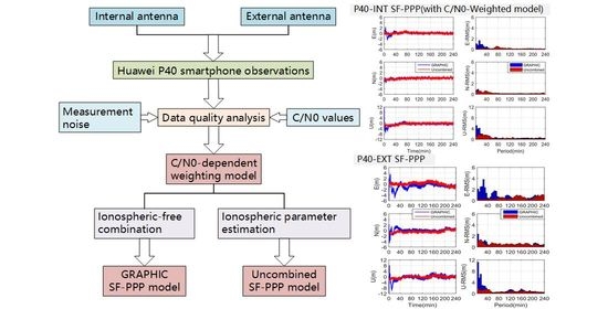
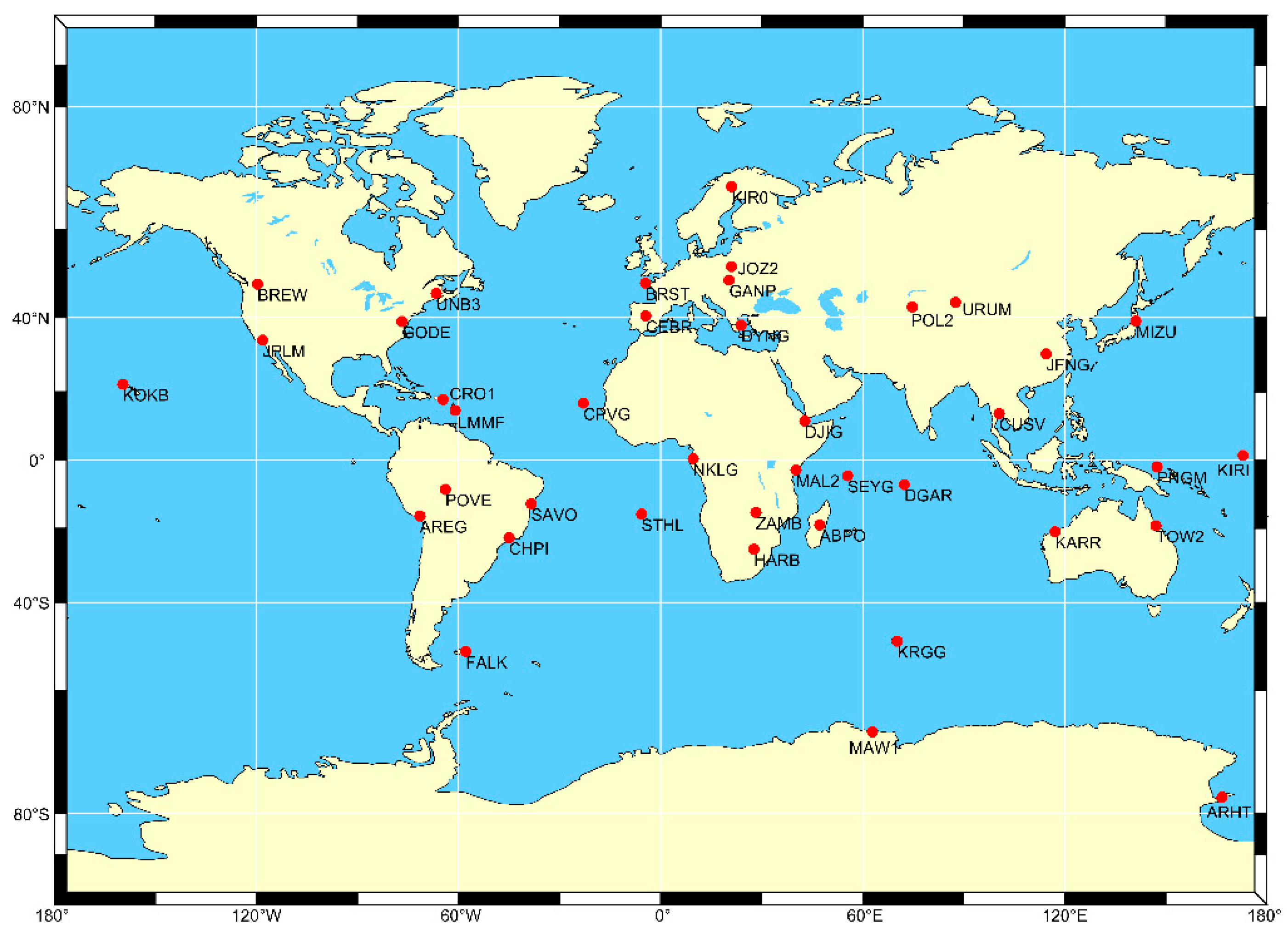
The focus of this study was to evaluate the performance of GRAPHIC and the uncombined SF-PPP approaches with datasets from Multi-GNSS Experiment (MGEX) stations as well as Huawei P40 smartphones. The MGEX stations, by providing geodetic-grade GNSS observations, can be treated as baselines for our SF-PPP assessment. The P40 can track dual or triple-frequency signals for different satellite systems, explicitly L1/L5 for GPS, B1I/B1C/B2a for BDS, E1/E5a for GALILEO, and L1/L5 for QZSS. However, the data continuity on the second frequency band (L5/B2a/E5a) was severely interrupted due to channel limitations, and only the measurements on the first frequency band were used for the investigation. We collected the P40 datasets both using its self-contained built-in antenna and an external geodetic antenna, thus making it possible to identify data quality problems caused by either the P40 chips or antennas. The paper is organized as follows. In Section 2, two kinds of SF-PPP models are elaborated by formulas and instructions. Then, the effectiveness of the positioning performance of the two models is examined by geodetic receivers in Section 3, both in terms of accuracy and convergence. In Section 4, first, we briefly describe a quality assessment that was conducted with the dataset collected by Huawei P40, and then the SF-PPP processing is examined. Finally, the conclusions are summarized in Section 5.

2. SF-PPP Methodology

The basic observational equation for SF-PPP is first presented in this section. Ionospheric delay is the main error source for SF-PPP, and the GRAPHIC and uncombined approaches are described in detail.

2.1. SF-PPP Observation Equations

For the receiver $r$ and satellite $s$, the basic observation equations of the pseudo-range and carrier phase on frequency $f$ can be formulated as:

$$\{\begin{array}{l}{P}_{r,f}^s={\rho }_r^s+cd{t}_r-cd{t}^s+T_r^s+Io{n}_{r,f}^s+c\left(d_{r,f}-d_f^s\right)+an{t}_{pco+pcv}+{\epsilon }_P\\ {\varphi }_{r,f}^s={\rho }_r^s+cd{t}_r-cd{t}^s+T_r^s-Io{n}_{r,f}^s+{\lambda }_f\left(N_{r,f}^s+b_{r,f}-b_f^s\right)+an{t}_{pco+pcv}+{\phi }_{\varphi }+{\xi }_{\varphi }\end{array},$$

(1)

where the ${\rho }_r^s$ denotes the geometric distance between the satellite and receiver in meters; $c$ denotes the speed of light; $d{t}_r$ and $d{t}^s$ are the clock offsets of the receiver and satellite, respectively; $T_r^s$ is the slant tropospheric delay in the satellite sight line direction; $Io{n}_{r,f}^s$ is the first-order slant ionospheric delay at the $f$ frequency (higher-order ionospheric delay are often at mm/cm level and can be ignored in SF-PPP); $d_{r,f}$ and $d_f^s$ are the frequency-dependent code hardware delay on receiver $r$ and satellite$s$, respectively; ${\lambda }_f$ is the wavelength of the frequency $f$ and $N_{r,f}^s$ is the carrier integer ambiguity; $b_{r,f}$ and $b_f^s$ are the frequency-dependent carrier phase hardware delay for receiver $r$ and satellite $s$, respectively; $an{t}_{pco+pcv}$ is the sum of the satellite and receiver antenna phase offsets and variations; ${\phi }_{\varphi }$ is the phase wind-up effect of phase observation; and ${\epsilon }_P$ and ${\xi }_{\varphi }$ are the sum of measurement noise and multipath error for the pseudorange and carrier phase, respectively. It should be noted that the inter-system bias (ISB) parameter should be considered when using multi-system observations.

The variances of raw code or phase measurements are assumed to be independent. The elevation-dependent stochastic model, which has been adopted in many studies [29,30] is applied as follows:

$$\{\begin{array}{c}{\sigma }_p^2=a^2/\left(4·{sin}^{2}e\right)\\ {\sigma }_L^2=b^2/\left(4·{sin}^{2}e\right)\end{array},$$

(2)

where $a$ and $b$ are the standard deviations for raw code and phase measurement noise, respectively (in this study, they are set as a = 0.3 m, b = 0.003 m), and $e$ is the elevation angle of the satellite [30].

2.2. GRAPHIC Model

Considering that the ionospheric delay of the pseudorange and carrier phase measurements have the same magnitude but opposite signs when ignoring the high-order terms, the GRAPHIC model can be formed as a linear combination by single-frequency of the pseudorange and carrier phase:

$$G_{r,f}^{s,Q}=\frac{P_{r,f}^{s,Q}+L_{r,f}^{s,Q}}{2}.$$

(3)

When implementing the GRAPHIC model, the carrier-phase observation in Equation (1) is replaced by $G_{r,f}^{s,Q}$ in Equation (3). For the GRAPHIC model, an a priori ionosphere background model is utilized for correcting the pseudorange observations. However, some mis-corrected ionospheric errors remain in pseudorange observations because of the accuracy limitation of the priori ionospheric model. It is worth noting that the noise level of the $G_{r,f}^{s,Q}$ observation in GRAPHIC approach is mainly affected by the pseudorange measurement precision, which may degrade the positioning accuracy and affect the convergence speed [34]. Thus, it is significant in the GRAPHIC model to improve the pseudorange measurement accuracy, which suffers mostly from ionospheric delay.

2.3. Uncombined Model

Unlike the GRAPHIC model, the raw pseudorange and carrier phase observations are utilized directly in the uncombined approach, while the slant ionospheric delays are estimated as random walk process parameters. In this way, the slant delay and receiver clock offset parameters are tightly coupled; thus, a priori constraint on the ionospheric parameters is a significant issue in improving both estimation accuracy and convergence. Explicitly, a priori ionosphere information provides approximate values for the epoch-wise slant delays and is then inserted into observation equations along with its variance information, which can be formulated as:

$$Io{n}_{r,f}^s=I_{r,f}^s,$$

(4)

$$I_{r,f}^s=40.28\times \frac{m·VTEC}{f^2},$$

(5)

$${\sigma }_{ion}^2={\sigma }_{ion\_k}^2/\left(4·{\mathit{sin}}^{2}e\right),$$

(6)

where $Io{n}_{r,f}^s$ is the ionospheric parameter with an approximate value $I_{r,f}^s$ derived by VTEC (vertical total electron content) and mapping function m, and ${\sigma }_{ion\_k}^2$ is the variance of $I_{r,f}^s$ at k-th epoch.

In this study, the GIM model provided by IGS was adopted when implementing both the GRAPHIC and uncombined models. The GIM can provide global ionosphere VTEC values over a 2 h temporal resolution and has a spatial resolution of 2.5° and 5° in latitude and longitude, respectively. The RMS of the GIM model is about 2–8 TECUs (total electron content units) [35]. Considering the accuracy limitation of GIM products, the slant delay observations $Io{n}_{r,f}^s$ are assigned with varying variances. Explicitly, ${\sigma }_{ion\_k}^2$ is assigned with a small value at the beginning stage of PPP processing to speed up estimation convergence as it can help decrease parameter correlations (such as the correlations between receiver clock errors, ambiguities, and ionospheric delays). However, ${\sigma }_{ion\_k}^2$ is then gradually increased as the initial ionospheric parameter values suffer errors from the GIM model; by loosening the ionospheric parameters constraints, the estimation precision could be improved [29]. The ${\sigma }_{ion\_k}^2$ can be expressed as:

$${\sigma }_{ion\_k}^2={\sigma }_{ion\_0}^2+\alpha \left(k-1\right)\mathsf{\Delta }t,$$

(7)

where ${\sigma }_{ion\_0}^2$ is the initial variance, set as 1.6 m² (standard deviation about 1.28 m); $\alpha$ is the variance varying rate with time, set as 1 ${\mathrm{m}}^2/\min$; and $\mathsf{\Delta }t$ is the elapsed time.

3. SF-PPP Performance Analysis of Multi-GNSS Stations

To evaluate the SF-PPP implementation, daily GNSS data from 40 globally distributed MGEX stations were processed during the days of the year 295–301 in October 2020. The geographical distribution of the experimental stations is shown in Figure 1.

3.1. SF-PPP Strategy

Pseudorange and carrier-phase observations on L1/E1/B1I frequencies were utilized. The Wuhan University multi-GNSS precise orbit and clock products (denoted as WUM products hereafter) [36] were employed. As the WUM products are generated with dual-frequency observation combination, differential code bias (DCB) errors should be corrected in SF-PPP. The multi-GNSS DCB products released by CAS (Chinese Academy of Science) were used. Both the phase center offsets (PCO) and phase center variations (PCV) of the receiver and satellite antennas were considered and corrected by the IGS antenna model. The satellite cutoff elevation angle was set to 10°. The hydrostatic tropospheric delay was calculated using the global pressure temperature (GPT) model [37]. The tropospheric wet delay was estimated as a process parameter with a prior variance of 0.5 m and process noise deviation of ${10}^{-5}m/\sqrt{s}$. To map the zenith tropospheric delay to slant delay, the global mapping function (GMF) was adopted [38]. Some other error terms such as relativistic time delay, phase windup, and station displacement were also considered. The detailed processing strategy and model corrections in SF-PPP are summarized in

Table 1. Strategies for SF-PPP.

Items	Processing Strategies
Navigation constellation	GPS/Galileo/BDS
Observations	Raw observations or GRAPHIC combinations
Frequency choices	L1/E1/B1I
Processing mode	Kinematic
Cutoff elevation angle	10°
Satellite orbit and clock	Fixed to precise products (WUM) [36]
Differential clock offset	MGEX DCB products (CAS)
PCO/PCV	Corrected by IGS ANTEX files (igs14.atx)
Receiver clock offset	Estimated as a random walk process
ISB	Estimated as a random walk process
Troposphere	Hydrostatic delay calculated by GPT [37] and GMF [38];Remaining wet delay estimated as a random walk process
Ambiguity	Estimated as a float constant
Station displacement	Solid earth tide, ocean tide, pole tide [39]
Relativistic time delay	Corrected
Phase windup	Corrected

.

3.2. Positioning Performance Analysis of Geodetic Receivers

The data from 40 global MGEX stations were processed using the GRAPHIC and uncombined SF-PPP approaches. Their weekly coordinate solutions from the IGS SINEX file were regarded as references to assess positional errors. To investigate the SF-PPP convergence, the RMS values of positioning errors every 5 min were also calculated.

Three stations at different latitudes were selected for illustration. As seen in Figure 2, the positioning errors and RMS values of GRAPHIC and uncombined models at the (a) MAL2 (low latitude), (b) JFNG (middle latitude), and (c) KIR0 (high latitude) stations on 26 October 2020 are presented. For each station, the left panels depict the time series of the positioning errors in the east (E), north (N), and up (U) components for the whole day period, respectively, while the right panels illustrate the RMS values every 5 min in each component for the first 4 h. Both the GRAPHIC and uncombined approaches achieved sub-meter positioning accuracy for these three stations. For the east and north components, the positioning precision reached at 0.1 m level, and 0.2 m for the vertical component. The MAL2 showed larger variations than the other two stations in all three components, which should be because the ionosphere activity was higher at low latitudes. The GRAPHIC and uncombined approaches exhibited different positioning convergence speeds. Comparatively, the uncombined model approach showed generally faster convergence than GRAPHIC, and its variations were much more stable. During the first 15 min, positioning errors of GRAPHIC SF-PPP even reached several meters, especially in the up direction, while the uncombined model was less than about 0.5 m and 1 m in the horizontal and vertical directions, respectively. This should be mainly attributed to the code and carrier phase combination in GRAPHIC approach being much noisier than the carrier phase observations in the uncombined approach.

To compare the overall convergence performance, the convergence times for all the 40 MGEX stations for the whole week were calculated. The convergence criteria were set as the positioning errors in the E, N, and U directions keeping less than 0.3 m, 0.3 m, and 0.5 m, respectively, for at least 10 min. In Figure 3, the distribution diagram of convergence time is depicted. It can be observed that the uncombined SF-PPP converged faster than GRAPHIC. For the results of the uncombined model, there was 55% for the east solutions, 40% for the north solutions, and 10% for the up solutions, which could converge within 5 min. In contrast, there were few solutions of the GRAPHIC model that could converge within 5 min.

The statistics of positioning errors after convergence and the average convergence time for all stations results are summarized in

Table 2. Statistical values of the positioning error and convergence time for the GRAPHIC model and the uncombined model.

			East	North	Up
Positioning error (m)	GRAPHIC	Mean	0.01	−0.01	−0.03
		STD	0.08	0.07	0.18
		RMS	0.08	0.08	0.18
	Uncombined	Mean	0.01	0.00	−0.03
		STD	0.08	0.07	0.16
		RMS	0.08	0.08	0.17
Convergence time (min)	GRAPHIC	Mean	30.3	18.1	30.2
	Uncombined	Mean	16.1	14.4	26.1

. In terms of positioning accuracy, both the GRAPHIC and uncombined SF-PPP approaches could reach accuracies of 0.1 m in the horizontal direction and 0.2 m in the vertical direction. A similar experiment was conducted in [30] with only GPS observations, and accuracies of 0.15 m and 0.3 m were obtained for the horizontal component and vertical component, respectively. This indicates that the fusion of the multi-GNSS system of GPS, BDS, and Galileo improves the positioning accuracy. The convergence times of the uncombined approach were 16.1, 14.4, and 26.1 min in the E, N, and U directions, respectively, which were significantly shorter than those for the GRAPHIC with convergence time of 30.3, 18.1, and 30.2 min, respectively. Compared to the GRAPHIC model, the convergence times of the uncombined model were improved by 40.7%, 20.0%, and 13.8% in the E, N, and U components, respectively. The reason the east component needed a longer convergence time than the north component can be explained by the satellite constellation configuration [29]. From the above investigation, it can be concluded that for geodetic receivers, both the GRAPHIC and uncombined SF-PPP approaches can obtain a positioning accuracy of about 0.1 m in the horizontal components and 0.2 m in vertical components, while the uncombined approach presents faster convergence speed.

4. SF-PPP Performance Analysis of Android Mobile Phones

The MGEX stations utilize geodetic-grade GNSS receivers, which provide better data quality than the Android devices and are beneficial to SF-PPP performance. In addition, currently, most mobile Android terminals usually cannot produce reliable and continuous dual-frequency or triple-frequency observations owing to the chip and antenna limitation; the SF-PPP technique is a more feasible approach for precise positioning or location-based applications. Thus, SF-PPP with Android smartphones is the focus of this section.

The Huawei P40 smartphone is adopted for this study, which utilizes Android release version 10.0 and the latest Kirin-990 chipset. It can track dual or triple-frequency signals for different satellite systems, explicitly L1/L5 for GPS, B1I/B1C/B2a for BDS, E1/E5a for GALILEO, and L1/L5 for QZSS. However, the data continuity on the second frequency band (L5/B2a/E5a) is severely interrupted owing to channel limitations. Thus, the data from the first frequency band are our focus. To avoid environmental impacts, we collected 4 h of data on the rooftop of a tall building inside Wuhan University at a sampling rate of 1 s on 26 October 2020. Two P40 smartphones were utilized to record GNSS measurements during the same period but with different antennas; one was the P40 built-in antenna, while the other was an external geodetic antenna (Huawei helped adapt the P40 for connection with external antennas). In this way, the impacts of the built-in antenna could be compared and analyzed. In this section, the quality of the GNSS observations from the smartphone is analyzed in terms of carrier-to-noise density ratio (C/N0), pseudorange noise, and carrier phase noise. Then, the result of SF-PPP is examined.

4.1. GNSS Data Quality Analysis of Mobile Devices

The C/N0 values obtained by the receiver indicate the signal gains and losses along the transmitting chain [40]. In general, the higher the C/N0 value, the stronger signal and the better observation quality that can be expected. Figure 4 shows the average C/N0 values of all satellites tracked by the P40 with external antenna (P40-EXT) and internal antenna (P40-INT) at different elevation bins to demonstrate the characteristics of C/N0 values for P40. For P40-EXT, the C/N0 values showed stable increments from about 30 dB-Hz to 45 dB-Hz with respect to satellite elevations; in addition, when satellite elevation was higher than 30 degrees, the P40-EXT C/N0 values were quite stable at around 45 dB-Hz. This was identical to the elevation-dependent stochastic model in Equation (2), where the observation weight was set to an equal weight model for the elevations higher than 30 degrees. In comparison, the P40-INT C/N0 values were overall smaller than P40-EXT and their difference was close to 10 dB-Hz. Especially, the P40-INT C/N0 showed large variations between 35 dB-Hz and 40 dB-Hz for elevations higher than 30 degrees and no significant correlations could be observed. This should be because the received signal strength of P40-INT was more susceptible to the environment with a linearly polarized non-uniform gain antenna [1,41].

The noise level of the pseudorange and carrier phase of P40 GNSS observations were evaluated by third-order between-epoch differences [3]. In Figure 5, the noise of P40-INT and P40-EXT pseudorange and carrier-phase are depicted for different GNSS systems over 4 h; the C/N0 are also illustrated to investigate their correlations. It should be noted that the selected periods are the same for different satellites, and the B1I and B1C signals for C36 are both illustrated as an insight on BDS-3 new signal evaluation with smartphones. As seen in Figure 5, the P40-INT data experienced large C/N0 variations from 25 dB-Hz to 40 dB-Hz. The G01 satellite from P40-INT showed the largest C/N0 variations, followed by E21. They exhibited a large C/N0 decrease over 60–80 min from approximately 40 dB-Hz to about 30 dB-Hz with a reduction as large as 12 and 10 dB-Hz, respectively. This should be attributed to signal acquisition incidents of the P40-INT devices, as such a decrease was not seen for P40-EXT. The E21 C/N0 also showed another minor decrease of 5 dB-Hz at around 40 min. However, the two BDS signals showed much smaller C/N0 fluctuations. Their C/N0 stayed at a rather lower C/N0 level (35 dB-Hz) during the first 60 min and then gradually grew to larger than 40 dB-Hz. Comparatively, the B1I C/N0 values were, overall, 2 dB-Hz larger than B1C. The P40-INT code triple-difference series showed strong correlations with respect to the C/N0 variations. The E21 and C36 code variations were within +/−3 m when their C/N0 stayed above 40 dB-Hz, while G01 were larger, at around +/−5 m. However, when C/N0 dropped below 30 dB-Hz, their variations amplified to about 10 m. The carrier-phase triple-differences mainly fluctuated around +/−0.5 cycles and barely showed any correlations with respect to C/N0. The P40-EXT C/N0 values manifested gradually variations, which were typically above 40 dB-Hz for elevations higher than 30 degrees. This was consistent with Figure 4. As result, the P40-EXT code triple-differences stayed stably within +/−3 m, while the carrier-phase was around +/−0.5 cycles.

To further analyze the relationship between the P40 measurement noise and elevation or the C/N0 value, Figure 6 shows the RMS values of triple-differences of pseudorange and carrier phase with different ranges of elevation and the C/N0 value for P40-EXT and P40-INT. The P40-INT dataset showed larger RMS values over all elevation bins for both the pseudorange and the carrier phase than the P40-EXT case, which should be attributed to the fact that the linearly polarized built-in antenna of P40-INT is more vulnerable to environmental interference leading to the larger observation noise. The pseudorange noise of P40-INT varied irregularly with the satellite elevation increment; however, it was more stable for P40-EXT. When the C/N0 value was lower than 25 dB-Hz, the pseudorange noise gradually reduced from 4 m to 2 m, showing good correlations, while the carrier-phase observations could not be tracked for both P40-INT and P40-EXT under such a C/N0 condition. However, when C/N0 increased to the range of 25–30 dB-Hz, the pseudorange noise from both P40-INT and P40-EXT manifested a dramatic increment to 5–6 m. To investigate such abnormal behavior, the recorded signal strength flags were checked, and it was found they were jumping between 1 and 4 constantly when C/N0 dropped below 30 dB-Hz, indicating an unstable tracking status. It was suspected that there were tracking problems owing to the P40 chips for C/N0 falling below 30 dB-Hz. Thus, in our subsequent SF-PPP processing, these measurements were discarded (the data volume for C/N0 below 30dB-Hz was only less than 5%). For C/N0 values higher than 30 dB-Hz, both the pseudorange and carrier phase noise showed a gradual decrease, and their triple-difference RMS values were at the level of 1 m and 0.1 cycles when C/N0 reached 48–50 dB-Hz, respectively. The correlations between the P40-INT pseudorange and carrier-phase noise with respect to C/N0 were much stronger than to the elevations; thus, constructing a C/N0-dependent weight model could be more appropriate in P40-INT positioning than an elevation-dependent one.

The GNSS measurement noises are derived from the above triple-difference RMS values by a normalization factor of $1/\sqrt{20}$ [3]. The P40 observation noise of different constellations is then calculated and shown in

Table 3. RMSs of pseudorange and carrier-phase noise for different smartphone antenna devices.

Devices	PseudorangeNoise RMS (m)
	GPS-L1	BDS-B1I	BDS-B1C	Galileo-E1	Average
P40-EXT	0.56	0.36	0.28	0.36	0.40
P40-INT	0.99	0.57	0.41	0.60	0.67
Devices	Carrier-Phase Noise RMS (cycle)
	GPS-L1	BDS-B1I	BDS-B1C	Galileo-E1	Average
P40-EXT	0.03	0.02	0.03	0.03	0.02
P40-INT	0.03	0.03	0.03	0.03	0.03

. The BDS B1C code noise was the smallest for both P40-EXT and P40-INT with values of 0.28 m and 0.41 m, respectively, while the GPS L1 was the largest with values of 0.56 m and 0.99 m, respectively. The BDS B1I and Galileo E1 showed very similar code noise levels at 0.40 m and 0.60 m, respectively. The noise level for different systems might be related to their C/N0 levels, as indicated in Figure 5. The average pseudorange noise values were 0.40 m and 0.67 m for P40-EXT and P40-INT, respectively, indicating about 70% improvement using an external geodetic antenna. For the carrier phase observations, the noise level of different GNSS systems were quite close to each other and their RMS values were 0.02 cycle and 0.03 cycle for P40-EXT and P40-INT, respectively.

4.2. Positioning Performance Analysis of Android Mobile Phones

Weak signal strength and high measurement noise present a great challenge to precise GNSS positioning for the smartphones. We further investigated the SF-PPP performance by utilizing the dataset collected from P40-EXT and P40-INT.

Figure 7 displays the number of available satellites (ASAT) as well as the position dilution of precision (PDOP) for different GNSS system combinations. The satellites used in SF-PPP solution are denoted as ASAT in the case of gross errors. With a geodetic-grade antenna, P40-EXT could generally track five more satellites than P40-INT. With multi-GNSS availability, the average number of ASAT of P40-EXT varied from 20 to 30 while that of P40-INT varied from 16 to 26, considering different frequency combinations. It should be noted five to six more BDS satellites could be observed at the B1I frequency than that at the B1C frequency for both P40-EXT and P40-INT. As a result, the PDOP of the GPS L1, BDS B1C, and Galileo E1 frequency combinations showed more dramatic changes than the case of using the B1I frequency, especially for P40-INT, where the PDOP even jumped from 0.9 to above 1.3. Although the B1C signal manifested a smaller code noise level than the B1I signal, it was still recommended to adopt the B1I signal to ensure more available satellites and better satellite geometry. With the GPS L1, BDS B1I, and Galileo E1 combination, the average GNSS ASAT numbers reached 27.3 and 23.9 for P40-EXT and P40-INT, respectively, while the resulting average PDOPs were 0.826 and 0.934, respectively.

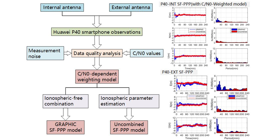
The P40-EXT positioning performance of the two SF-PPP approaches was evaluated using observations from GPS L1, BDS B1I, and Galileo E1 frequencies. The left panel of Figure 8 shows the epoch-wise positioning errors in the east, north, and up components for the GRAPHIC and uncombined solutions of P40-EXT, while the right panel is the corresponding RMS values every 5 min. The positioning errors of the GRAPHIC and uncombined approaches were at the same order of magnitude; both could reach sub-meter level positioning accuracy after convergence. However, the uncombined model had a slightly higher accuracy in the up component. When the GRAPHIC approach was applied, the positioning errors of P40-EXT were within a few meters during the first 20 min, and it took about 40 min to stabilize. In contrast, the uncombined model could achieve accuracy within 1 m in the horizontal direction and 2 m in the vertical direction during a few minutes. The remarkable improvement in terms of convergence performance of the uncombined model should be attributed to the fact that the carrier phase observation precision is much higher than the GRAPHIC combination and that the ionospheric parameters could absorb part of observational errors.

Considering the code noise correlation with respect to C/N0, the P40-INT SF-PPP was evaluated using a C/N0-dependent weighting model in addition to the elevation-dependent model for comparison. The C/N0-dependent weighting model was represented in an exponential form related to the instantaneous C/N0 of the observations, a maximum C/N0 value for cutoff, and the corresponding pseudorange noise at maximum C/N0. Its detailed expression could be found in [42]. Considering the P40-INT noise analysis results in Section 4.1, the C/N0-dependent weighting model was adapted by setting the maximum C/N0 cutoff as 40 dB-Hz and the corresponding pseudorange noise 1 m. The positioning errors are shown in Figure 9a,b. Generally, the positioning errors of P40-INT varied abruptly and needed a longer convergence time for both SF-PPP approaches and for both weight models than P40-EXT. Considering the elevation-dependent weighting model, both the GRAPHIC and uncombined approaches manifested large variations around ±2 m in the horizontal component and ±6 m in the vertical component even after convergence; very similar systematic errors could be observed for both approaches, which might be due to some systematic observation errors and remains under investigation. Comparatively, the uncombined approach showed smaller positioning errors, especially at the vertical component. With the C/N0-dependent weighting model, the P40-INT positioning results showed a significant improvement over the elevation-dependent model for both SF-PPP approaches with smaller variations. Especially, the vertical error variations were within ±4 m. However, the systematic errors were still found.

The histograms of P40-EXT and P40-INT SF-PPP positioning errors during the last 120 min are shown in Figure 10. In Figure 10a, it could be seen that the GRAPHIC positioning errors of the P40-EXT case achieved comparable performance with the uncombined method. Their horizontal fluctuations varied within $\pm$0.5 m and their RMS values varied around 0.15 m. However, the uncombined approach showed much smaller errors in the vertical component with an improvement of about 30%, consistent with Figure 8. Figure 10b,c depict the P40-INT SF-PPP errors using the elevation-dependent weighting model and the C/N0-dependent weighting model, respectively. Generally, the uncombined method overperformed the GRAPHIC method in the vertical component with dramatic improvements; for the elevation-dependent weighting model, the RMS reduction was about 1.40 m, while for C/N0-dependent model it was about 0.24 m. Their horizontal precisions were at a similar level below 1.0 m. Compared to the elevation-dependent weighting model, the C/N0-dependent model showed much better vertical precision at 0.66 m.

Figure 11 summarizes the SF-PPP positioning results in each coordinate component of P40-EXT (left panel bars) and P40-INT. For P40-INT, the results of both the elevation-dependent weighting method (middle panel bars) and the C/N0-dependent weighting (right panel bars) are shown. The statistical values are based on the positioning results after 120 min, when the series vary stably. In the case of P40-EXT, the GRAPHIC and uncombined models of the smartphone reached comparable accuracies of about 0.15 m in horizontal components, while the uncombined model achieved 0.33 m in the vertical component that was better than the GRAPHIC model (0.48 m), indicating an improvement of about 31%. In addition, biases at a few centimeters level in the horizontal components and several decimeters level at the vertical component could be observed for both approaches, which was different compared to the results of MGEX stations. This again indicated that there were systematic errors in the P40 measurements. For the P40-INT case, the positioning errors of the GRAPHIC model with the elevation-dependent weighting strategy were 0.74 m, 0.42 m, and 2.35 m in the east, north, and up components, respectively. However, with the C/N0-dependent weighting approach, the errors were decreased to 0.65 m, 0.42 m, and 0.90 m, respectively; an improvement as large as 62% could be observed in the vertical component. For the uncombined approach using the C/N0-dependent weighting method, the east, north, and vertical errors were 0.72 m, 0.51 m, and 0.66 m, respectively. The vertical component exhibited an improvement of about 27% compared with the GRAPHIC model, while the horizontal component showed little degradation.

The above results indicate that the uncombined approach could achieve better positioning precisions compared to the GRAPHIC model for P40 smartphones with either built-in or external antennas. For P40 GNSS data with its built-in antenna, the C/N0-dependent weighting strategy is more suitable and can improve positioning precision. Sub-meter level accuracy could be reached after about 1 h.

5. Discussion and Conclusions

In this study, the positioning performance of GRAPHIC and uncombined SF-PPP models was evaluated and compared. We firstly evaluated these two approaches using one-week datasets from 40 MGEX stations in case of any observational quality issues. The two approaches achieved very similar positioning accuracy, with 0.1 m and 0.2 m in the horizontal and vertical directions, respectively. However, the uncombined approach manifested faster convergence than GRAPHIC by 40.7%, 20.0%, and 13.8% in the east, north, and up components, respectively, owing to the adoption of high-precision carrier phase observations as well as ionospheric parameterization.

We collected smartphone-based datasets using the Huawei P40 smartphone equipped with an external geodetic-grade antenna (P40-EXT) as well as its internal antenna (P40-INT) for comparison and analysis. Firstly, the raw observations from these two smart devices were compared in terms of the C/N0 value and measurement noise. The code measurement noise with the internal antenna case were 0.27 m larger than the external, while little differences were found for carrier phase observations. In addition, the P40-INT pseudorange noise showed strong correlations with respect to the C/N0 values. The P40 observations from the GPS L1, BDS B1I, and Galileo E1 frequencies were utilized to conduct SF-PPP. The errors of uncombined SF-PPP of the external antenna case were 0.14 m, 0.15 m, and 0.33 m in the east, north, and up components, respectively, showing an improvement of about 31% in the up direction when compared with the GRAPHIC solution. The C/N0-dependent weighting model performed much better than the elevation-dependent model for the internal antenna case with an improvement of about 30–60%, especially in the vertical component. It improved the GRAPHIC positioning accuracy to 0.65 m, 0.42 m, and 0.90 m in the east, north, and up directions, respectively, and for the uncombined approach, the precision could even reach 0.72 m, 0.51 m, and 0.66 m in the east, north, and up directions, respectively.

References

1. Zhang, X.; Tao, X.; Zhu, F.; Shi, X.; Wang, F. Quality assessment of GNSS observations from an Android N smartphone and positioning performance analysis using time-differenced filtering approach. GPS Solut. 2018, 22, 1–11. [Google Scholar] [CrossRef]
2. Liu, W.; Shi, X.; Zhu, F.; Tao, X.; Wang, F. Quality analysis of multi-GNSS raw observations and a velocity-aided positioning approach based on smartphones. Adv. Space Res. 2019, 63, 2358–2377. [Google Scholar] [CrossRef]
3. Li, G.; Geng, J. Characteristics of raw multi-GNSS measurement error from Google Android smart devices. GPS Solut. 2019, 23, 1–16. [Google Scholar] [CrossRef]
4. Robustelli, U.; Baiocchi, V.; Pugliano, G. Assessment of Dual Frequency GNSS Observations from a Xiaomi Mi 8 Android Smartphone and Positioning Performance Analysis. Electronics 2019, 8, 91. [Google Scholar] [CrossRef] [Green Version]
5. Håkansson, M. Characterization of GNSS observations from a Nexus 9 Android tablet. GPS Solut. 2018, 23, 21. [Google Scholar] [CrossRef] [Green Version]
6. Pesyna, K.M.; Heath, R.W.; Humphreys, T.E. Centimeter Positioning with a Smartphone-Quality GNSS Antenna. In Proceedings of the 27th International Technical Meeting of the Satellite Division of The Institute of Navigation (ION GNSS+, 2014), Tampa, FL, USA, 8–12 September 2014; pp. 1568–1577. [Google Scholar]
7. Pesyna, K.M.; Humphreys, T.E.; Heath, R.W.; Novlan, T.D.; Zhang, J.C. Exploiting Antenna Motion for Faster Initialization of Centimeter-Accurate GNSS Positioning With Low-Cost Antennas. IEEE Trans. Aerosp. Electron. Syst. 2017, 53, 1597–1613. [Google Scholar] [CrossRef]
8. Paziewski, J.; Sieradzki, R.; Baryla, R. Signal characterization and assessment of code GNSS positioning with low-power consumption smartphones. GPS Solut. 2019, 23, 98. [Google Scholar] [CrossRef] [Green Version]
9. Geng, J.; Li, G. On the feasibility of resolving Android GNSS carrier-phase ambiguities. J. Geod. 2019, 93, 2621–2635. [Google Scholar] [CrossRef]
10. Realini, E.; Caldera, S.; Pertusini, L.; Sampietro, D. Precise GNSS Positioning Using Smart Devices. Sensors 2017, 17, 2434. [Google Scholar] [CrossRef] [Green Version]
11. Dabove, P.; di Pietra, V. Towards high accuracy GNSS real-time positioning with smartphones. Adv. Space Res. 2019, 63, 94–102. [Google Scholar] [CrossRef]
12. Dabove, P.; di Pietra, V. Single-Baseline RTK Positioning Using Dual-Frequency GNSS Receivers Inside Smartphones. Sensors 2019, 19, 4302. [Google Scholar] [CrossRef] [Green Version]
13. Zumberge, J.F.; Heflin, M.B.; Jefferson, D.C.; Watkins, M.M.; Webb, F.H. Precise point positioning for the efficient and robust analysis of GPS data from large networks. J. Geophys. Res. Solid Earth 1997, 102, 5005–5017. [Google Scholar] [CrossRef] [Green Version]
14. Kouba, J.; Héroux, P. Precise Point Positioning Using IGS Orbit and Clock Products. GPS Solut. 2001, 5, 12–28. [Google Scholar] [CrossRef]
15. Chen, B.; Gao, C.; Liu, Y.; Sun, P. Real-time Precise Point Positioning with a Xiaomi MI 8 Android Smartphone. Sensors 2019, 19, 2835. [Google Scholar] [CrossRef] [Green Version]
16. Wang, G.; Bo, Y.; Yu, Q.; Li, M.; Yin, Z.; Chen, Y. Ionosphere-Constrained Single-Frequency PPP with an Android Smartphone and Assessment of GNSS Observations. Sensors 2020, 20, 5917. [Google Scholar] [CrossRef]
17. Elmezayen, A.; El-Rabbany, A. Precise Point Positioning Using World’s First Dual-Frequency GPS/GALILEO Smartphone. Sensors 2019, 19, 2593. [Google Scholar] [CrossRef] [Green Version]
18. Wu, Q.; Sun, M.; Zhou, C.; Zhang, P. Precise Point Positioning Using Dual-Frequency GNSS Observations on Smartphone. Sensors 2019, 19, 2189. [Google Scholar] [CrossRef] [PubMed] [Green Version]
19. Aggrey, J.; Bisnath, S.; Naciri, N.; Shinghal, G.; Yang, S. Multi-GNSS precise point positioning with next-generation smartphone measurements. J. Spat. Sci. 2019, 65, 79–98. [Google Scholar] [CrossRef]
20. Øvstedal, O. Absolute Positioning with Single-Frequency GPS Receivers. GPS Solut. 2002, 5, 33–44. [Google Scholar] [CrossRef]
21. Klobuchar, J.A. Ionospheric Time-Delay Algorithm for Single-Frequency GPS Users. IEEE Trans. Aerosp. Electron. Syst. 1987, AES-23, 325–331. [Google Scholar] [CrossRef]
22. Schaer, S. Mapping and Predicting the Earth’s Ionosphere Using the Global Positioning System; Technische Hochschule Zürich: Zürich, Switzerland, 1999. [Google Scholar]
23. Yunck, T.P. Coping with the Atmosphere and Ionosphere in Precise Satellite and Ground Positioning; Advancing Earth and Space Science: Washington, DC, USA, 1993. [Google Scholar]
24. Andrei, C.O.; Chen, R.; Kuusniemi, H.; Hernandez-Pajares, M.; Sanz, J. Ionosphere Effect Mitigation for Single-frequency Precise Point Positioning. In Proceedings of the 22nd International Technical Meeting of the Satellite Division of The Institute of Navigation (ION GNSS 2009), Savannah, GA, USA, 22–25 September 2009; pp. 2508–2517. [Google Scholar]
25. Sterle, O.; Stopar, B.; Pavlovčič Prešeren, P. Single-frequency precise point positioning: An analytical approach. J. Geod. 2015, 89, 793–810. [Google Scholar] [CrossRef]
26. Montenbruck, O. Kinematic GPS positioning of LEO satellites using ionosphere-free single frequency measurements. Aerosp. Sci. Technol. 2003, 7, 396–405. [Google Scholar] [CrossRef]
27. Choy, S.; Silcock, D. Single Frequency Ionosphere-free Precise Point Positioning: A Cross-correlation Problem? J. Geod. Sci. 2011, 1, 314–323. [Google Scholar] [CrossRef]
28. Shi, C.; Gu, S.; Lou, Y.; Ge, M. An improved approach to model ionospheric delays for single-frequency Precise Point Positioning. Adv. Space Res. 2012, 49, 1698–1708. [Google Scholar] [CrossRef]
29. Cai, C.; Gong, Y.; Gao, Y.; Kuang, C. An Approach to Speed up Single-Frequency PPP Convergence with Quad-Constellation GNSS and GIM. Sensors 2017, 17, 1302. [Google Scholar] [CrossRef] [PubMed] [Green Version]
30. Li, B.; Zang, N.; Ge, H.; Shen, Y. Single-frequency PPP models: Analytical and numerical comparison. J. Geod. 2019, 93, 2499–2514. [Google Scholar] [CrossRef]
31. Gill, M.; Bisnath, S.; Aggrey, J.; Seepersad, G. Precise Point Positioning (PPP) using Low-Cost and Ultra-Low-Cost GNSS Receivers. In Proceedings of the 30th International Technical Meeting of The Satellite Division of the Institute of Navigation (ION GNSS+ 2017), Portland, OR, USA, 25–29 September 2017. [Google Scholar]
32. Laurichesse, D.; Rouch, C.; Marmet, F.X.; Pascaud, M. Smartphone Applications for Precise Point Positioning. In Proceedings of the 30th International Technical Meeting of The Satellite Division of the Institute of Navigation (ION GNSS+ 2017), Portland, OR, USA, 25–29 September 2017. [Google Scholar]
33. Geng, J.; Jiang, E.; Li, G.; Xin, S.; Wei, N. An Improved Hatch Filter Algorithm towards Sub-Meter Positioning Using only Android Raw GNSS Measurements without External Augmentation Corrections. Remote Sens. 2019, 11, 1679. [Google Scholar] [CrossRef] [Green Version]
34. Cai, C.; Liu, Z.; Luo, X. Single-frequency Ionosphere-free Precise Point Positioning Using Combined GPS and GLONASS Observations. J. Navig. 2013, 66, 417–434. [Google Scholar] [CrossRef] [Green Version]
35. Choy, S.; Zhang, K.; Silcock, D. An Evaluation of Various Ionospheric Error Mitigation Methods used in Single Frequency PPP. J. Glob. Position 2008, 7, 62–71. [Google Scholar] [CrossRef] [Green Version]
36. Guo, J.; Xu, X.; Zhao, Q.; Liu, J. Precise orbit determination for quad-constellation satellites at Wuhan University: Strategy, result validation, and comparison. J. Geod. 2015, 90, 143–159. [Google Scholar] [CrossRef]
37. Boehm, J.; Heinkelmann, R.; Schuh, H. Short Note: A global model of pressure and temperature for geodetic applications. J. Geod. 2007, 81, 679–683. [Google Scholar] [CrossRef]
38. Boehm, J.; Niell, A.; Tregoning, P.; Schuh, H. Global Mapping Function (GMF): A new empirical mapping function based on numerical weather model data. Geophys. Res. Lett. 2006, 33, L07304. [Google Scholar] [CrossRef] [Green Version]
39. Liu, J.N.; Ge, M.R. PANDA software and its preliminary result of positioning and orbit determination. Wuhan Univ. J. Nat. Sci. 2003, 8, 603–609. [Google Scholar]
40. Hauschild, A.; Montenbruck, O.; Sleewaegen, J.-M.; Huisman, L.; Teunissen, P.J.G. Characterization of Compass M-1 signals. GPS Solut. 2011, 16, 117–126. [Google Scholar] [CrossRef]
41. Humphreys, T.E.; Murrian, M.; Diggelen, F.V.; Podshivalov, S.; Pesyna, K.M. On the feasibility of cm-accurate positioning via a smartphone’s antenna and GNSS chip. In Proceedings of the Position, Location & Navigation Symposium, Savannah, GA, USA, 11–16 April 2016. [Google Scholar]
42. Wang, L.; Li, Z.; Wang, N.; Wang, Z. Real-time GNSS precise point positioning for low-cost smart devices. GPS Solut. 2021, 25, 69. [Google Scholar] [CrossRef]
Figure 1. Geographical distribution of 40 MGEX stations.
Remotesensing 13 04894 g001
Figure 2. Positioning errors (left panel) and RMS values of errors every 5 min (right panel) in the first 4 h during the test period of SF-PPP solutions at the (a) MAL2, (b) JFNG, and (c) KIR0 stations.
Remotesensing 13 04894 g002
Figure 3. Distribution of convergence time for the GRAPHIC model and the uncombined model in the E, N, and U directions, from top to bottom.
Remotesensing 13 04894 g003
Figure 4. Mean C/N0 values of all satellites tracked by different smartphone antenna devices at different elevation bins. The elevation interval is 2 degrees.
Remotesensing 13 04894 g004
Figure 5. Pseudorange noise and C/N0 (left panel) and carrier-phase noise (right panel) of the observations on G01 L1 frequency (a), C36 B1I frequency (b), C36 B1C frequency (c), and E21 E1 frequency (d) for different smartphone antenna devices.
Remotesensing 13 04894 g005
Figure 6. Pseudorange (left panel) and carrier-phase (right panel) noise RMS versus satellite elevation (top panel) and C/N0 value (below panel) for different smartphone antenna devices.
Remotesensing 13 04894 g006
Figure 7. The number of available satellites and the PDOP in different smartphone antenna devices.
Remotesensing 13 04894 g007
Figure 8. Positioning errors (left panel) and RMS values of errors every 5 min (right panel) of the SF-PPP solutions for P40 smartphone with an external antenna.
Remotesensing 13 04894 g008
Figure 9. Positioning errors (left panel) and RMS values of errors every 5 min (right panel) of the SF-PPP solutions for P40 smartphone with the internal antenna using the elevation-dependent weight model (a) and the C/N0-dependent weight model (b).
Remotesensing 13 04894 g009
Figure 10. Histograms of the SF-PPP positioning errors during the last 120 min for cases.
Remotesensing 13 04894 g010
Figure 11. Statistical values of positioning errors for different smartphone devices of the SF-PPP result series at the end of 120 min.
Remotesensing 13 04894 g011