
Down-Looking Airborne Radar Imaging Performance: The Multi-Line and Multi-Frequency


Institute for Electromagnetic Sensing of the Environment (IREA), National Research Council (CNR), 80124 Napoli, Italy
*
Author to whom correspondence should be addressed.
Remote Sens. 2021, 13(23), 4897; https://0-doi-org.brum.beds.ac.uk/10.3390/rs13234897
Submission received: 20 October 2021
/
Revised: 23 November 2021
/
Accepted: 29 November 2021
/
Published: 2 December 2021
(This article belongs to the Special Issue Airborne Synthetic Aperture Radar: Systems, Processing, New Challenges and Opportunities)
Abstract
:The paper proposes an analytical study regarding airborne radar imaging performances and accounts for a down-looking radar system moving along parallel lines far, in terms of probing wavelength, from the investigated domain and collecting multi-frequency and multi-monostatic data. The imaging problem is formulated in a constant depth plane by exploiting the Born approximation. Hence, a linear inverse scattering problem is faced by considering both the Adjoint and the Truncated Singular Value Decomposition reconstruction schemes. Analytical and simulated results are provided to state how the achievable performances depend on the measurement configuration. These results are of practical usefulness because, in operative conditions, it is unfeasible to plan a flight grid made up by a high number of closely (in terms of probing wavelength) spaced lines. Hence, the understanding of how the availability of under-sampled data affects the radar imaging allows for a trade-off between operative data collection constrains and reliable reconstructions of the scenario under test.
1. Introduction
Radar systems mounted on airborne platforms like small unmanned aerial vehicles (UAVs) are worth being considered because UAV allows for a not trivial simplification of the measurement logistic phase. UAV makes, indeed, possible an easy access to areas, which are hard to be reached by human operators or dangerous for them, and it permits the survey of wide areas without efforts. Accordingly, different kind of UAV-based down-looking radar systems have been recently proposed [1,2,3,4,5,6,7,8], someone of them working at high frequency and applied for landmine detection [2,3,4,5,7] and cultural heritage [8].
Whatever is the considered radar system and the application of interest, a common issue is the design of the measurement configuration as a function of the flight parameters, i.e., flight altitude, number of measurement lines, and number of measurement points along each line. The radar imaging result depends, indeed, on the amount and quality of data as well as on the adopted data processing strategy [9,10]. Moreover, when a UAV radar system is employed, one must account for that, in practice, it is unfeasible to plan a flight grid with a high number of lines spaced by a small, in terms of probing wavelength, spatial offset. Therefore, it is clear that an open practical issue is to understand how the imaging capabilities depend on the measurement setup.
A contribution to this topic has been given in [11], where analytical and numerical results have been presented for the case of single frequency, multi-lines, multi-monostatic data. Specifically, in [11] a radar moving along parallel lines at a certain altitude and collecting single frequency data at nadir has been considered. In addition, the imaging has been formulated in the 2D (x-y) plane under the Born approximation [12], and the Truncated Singular Values Decomposition (TSVD) approach [13] has been adopted as inversion procedure.
In this paper, the same measurement configuration and assumptions of [11] are made but, differently from [11], multi-frequency data are exploited. Moreover, the imaging capabilities of the Adjoint and the TSVD reconstruction approaches [13] are investigated. The analysis is performed by accounting for the Point Spread Function (PSF) as a tool to foresee the effect of the measurement configuration on the achievable spatial resolution along x and y directions. Analytical results are firstly derived. After, numerical results, referred to a wide-band high frequency radar system, are presented to show the benefits introduced by the availability of multi-frequency data and to compare the performance of the two considered inversion approaches.
The paper is organized as follows. Section 2 deals with the formulation of the imaging problem and recalls the inversion procedures. Section 3 provides analytical results stating how multi-frequency multi-monostatic well and under-sampled data affect the imaging capabilities in terms of spatial resolution and occurrence of grating lobes. Numerical results concerned with a point-like target are presented in Section 4, while the case of an extended target is tackled in Section 5. Conclusions are given in Section 6.
2. Imaging Problem
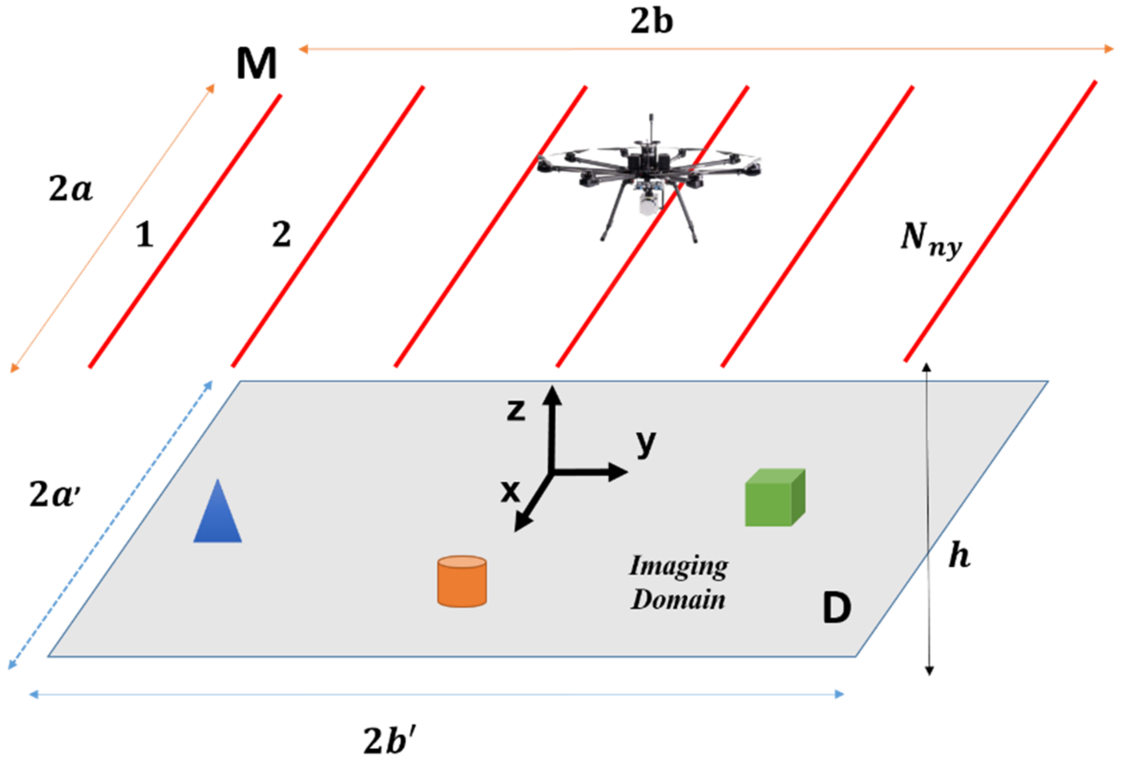
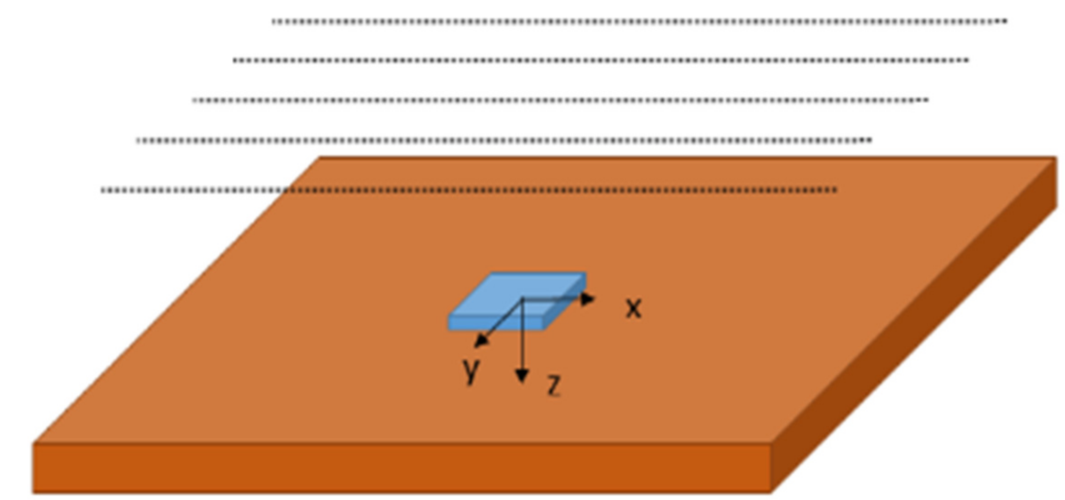
Let us consider the imaging scenario depicted in Figure 1. A radar system, mounted on a UAV platform, collects data over the planar surface M = (−a, a) × (−b, b) by traveling along parallel measurement lines with . The measurement lines are parallel to the x-axis, evenly spaced along the y-axis and at a constant altitude h above the imaging surface. This latter is the spatial domain D = (−a’, a’) × (−b’, b’) located at z = 0. The radar operates in monostatic mode and illuminates the scene at nadir (i.e., along z-axis) at each measurement point . The transmitting and receiving antennas are modeled as wide-band linear dipoles, oriented along the y-axis and operating at a central frequency belonging to the C-band. The targets are located into the imaging domain D.
Under the above assumptions and considering the Born Approximation, the scattering phenomenon is described in the frequency domain by the following linear integral equation:
In Equation (1), denotes the collected component of the backscattered field at the measurement point and at the angular frequency ; is the free-space propagation constant ( and being the free-space magnetic permeability and dielectric permittivity, respectively). Moreover, is the unknown contrast function, being the dielectric permittivity function at the generic point in D; is the dyadic Green function in free space; while is the incident filed, whose expression is:
where is the transmitting dipole current moment and is the free-space impedance.
The start and stop approximation is assumed, i.e., the radar is considered motionless (at a fixed measurement point ) in the time interval between the transmission of the probing signal, i.e., the incident field, and the reception of the corresponding backscattered field.
Let the radar operate in far-field [12], by substituting Equation (2) in Equation (1) and exploiting the far field expression of the Greens function, the scattering equation is rewritten as:
where the dependency on has been omitted. , , and is the linear scattering operator mapping the unknown space into data space, where denotes the space of the square integrable functions and is the radar frequency band, and being the minimum and maximum angular frequencies, respectively.
To face the imaging problem as defined by Equation (3), two reconstruction strategies are considered: the Adjoint procedure [13] and the Truncated Singular Value Decomposition (TSVD) inversion scheme [13]. These approaches allow for a closed form expression of the contrast function given in terms of the SVD of the discretized version of the operator . Specifically, after discretization, the imaging is faced as the solution of the matrix inverse problem:
where is the N-dimensional data vector, is the Q-dimensional unknown vector, Q being the number of points in D, and is the N × Q-dimensional matrix obtained by discretizing the integral operator . Let be the singular system of the matrix , we have [13]:
where denotes the adjoint matrix, are the singular values in decreasing order, while and define the orthonormal basis of the object space and the data space, respectively.
By exploiting the SVD representation of , the estimated contrast function is expressed as:
according to the Adjoint procedure, and as
according to the TSVD approach. In Equations (6) and (7), is the scalar product; the parameter in Equation (6) is the amount of collected data, while the parameter in Equation (7) is the regularization threshold [13]. The modulus of the contrast function as defined by Equation (6) or Equation (7) is the tomographic image of the scenario under test.
3. Imaging Performance Analysis
This Section aims at providing analytical results relating the imaging capabilities to the measurement configuration. These results are propaedeutic to the outcomes of the numerical analysis presented in the following sections. In detail, with respect to the imaging scenario sketched in Figure 1, this Section discusses about the amount of independent data, i.e., the minimum number of samples required to represent the backscattered field properly, as well as the achievable spatial resolution limits and the occurrence of grating lobes.
The analysis deals with the far field condition and, as previously done in [11] for the single frequency case, it starts with the assumption that both the frequency range and the measurement domain M are sampled continuously. Thereafter, it takes into account that a dense sampling is reasonable for and the along-track direction, i.e., the x-axis for the scenario at hand (see Figure 1), whereas it is practically unfeasible for the across direction, i.e., the y-axis. The sampling measurement step along y-axis, indeed, must be compliant with the positioning accuracy reachable by the on-board Global Navigation Units (GNUs), which control the UAV flight trajectory. Consequently, a coarse measurement step is expected along the y-axis. The discrete sampling case is distinguished by considering: (i) data sampled in agreement with the Nyquist criterion (i.e., well sampled data) and (ii) under sampled data.
3.1. Continuous Sampling
Based on the far field condition, we assume , and In this case, by applying the paraxial approximation [14] the distance term appearing in the exponential term of Equation (3) is expressed as:
and Equation (3) is rewritten as:
The kernel of the integral in Equation (9) is separable and we can tackle the dependence on the spatial variables independently. Let us start by considering the variable and the equation:
Let be , and , Equation (10) is rewritten as:
where . Equation (11) is the Fourier Transform (FT) of the contrast function , which has the spatial limited support .
According to the Nyquist criterion, the sampling step of the FT of a spatial limited function in is [13]. On the other hand, it is easy to verify that in the multi-monostatic and multi-frequency case herein at hand, the variable takes values into the range , where is the minimum wavelength. Hence, it follows that the number of samples required to represent is given by [15,16]:
By repeating the same reasoning for the spatial variable y’, the minimum number of samples to represent is:
Therefore, the total number of multi-monostatic and multi-frequency data required to represent the scattered field, while assuring no loss of information, is:
It is worth pointing out that the Nyquist sample number, as given by Equation (14), defines the amount of not redundant samples necessary to represent the backscattered field. However, it does not provide a practical rule to properly set the number of measurement points on M, i.e., along x and y axes, as well as the number of frequencies in . Indeed, although , and are independent variables, there is an infinite number of their combinations which satisfies the Nyquist criterion for sampling and . On the other hand, an evenly sampling of the measurement domain M, along x and y, as well as of the frequency range , can provide an insufficient amount of independent samples of the backscattered field even if the gathered number of data is equal or higher than the Nyquist number.
3.2. Discrete Sampling: Resolution Limits and Grating Lobes
Let us assume that the backscattered field is measured at a finite number of angular frequencies with in the range and at a finite number of evenly spaced points on M with and . Moreover, and denote the amount of multi-monostatic and multi-frequency data collected along the x-axis and the y-axis, respectively. As in the previous Section, we consider the dependence on the two spatial variables independently and start by considering the variable. Hence, let , , and we have:
3.2.1. Nyquist Sampling Configuration
Let us consider defined in Equation (12). In this case, the samples are the Fourier harmonics of and the solution of the inverse problem in Equation (15) has the following expression:
being . In order to appreciate the spatial resolution, we use Equation (16) to calculate the Point Spread Function (PSF) referred to a point like target located a . By means of some matematical passages, which are not reported for sake of brevity, it is obtained the following expression [11]:
The PSF in Equation (17) depends on by means of the quantity , it is maximum at and it has its first null is at:
This means that the spatial resolution limit along the x-axis is dictated by the maximum frequency of the considered range and depends on the flight altitude h.
Note that the modulus of the PSF in Equation (17) has period with respect to the variable . Hence, grating lobes occurr at with .
All the above considerations are valid also for , provided that is replaced by , by and by . Hence, with respect to , the PSF is given by
while the 2D PSF is expressed as:
It is worth pointing out that, while the spatial resolution limits along and do not depend on and , these latter affect the imaging capabilities due to the possible occurrence of grating lobes. In the case at hand, and are given by Equations (12) and (13), respectively, hence and while the parameters and get the values:
Consequently, since grating lobes occurr when and with , they are at and , which are points outside the investigated domain. In other words, as it is obvious, the Nyquist sample number assures that no aliasing effects occurr.
3.2.2. Undersampling Configuration
Let us consider that the data are collected according to the Nyquist criterion along the UAV travelling direction, i.e., the -axis, while under-sampled data are collected along the across direction, i.e., the -axis. As said at the beginning of this Section, this is compliant with the fact that a large amount of measurement points is feasible along the -axis, while practical flight constrains make unfeasible to consider a large number of dansly spaced measurement lines. Hence, in practice, an often encountered condition is the availabilty of an amount of data such that .
Let us express the sampling step as , being an auxiliary spatial parameter such that The amount of backscattered field samples is given by . In this case, the resolution limits do not change because they do not depend on ; conversely, grating lobes occur at:
and alsiaing issues arise.
4. Performance Analysis
This Section investigates how the imaging capabilities of the Adjoint procedure and the TSVD regularization scheme (see Section II) depend on the adopted measurement configuration. The analysis deals with spatial resolution limits and occurrence of grating lobes. In particular, a point-like target centered in , i.e., at the origin of the reference system given in Figure 1, is considered. The imaging domain, D, is a square located at z = 0 m whose side is 3 m long, i.e., m. The data are gathered in the frequency range GHz by a UAV mounted radar. The latter covers a measurement domain M, which is a square with sides 3 m long, and it travels at height h along multiple measurement lines parallel to the -axis. Three examples are considered and are referred to as Example A, B and C.
4.1. Example A (Height of the Platform Equal to 15 m)
Let us assume that the flight altitude is h = 15 m. According to the above definition of D, M and and the analytical results given in Section 3, we have =18, the spatial resolution is expected to be 0.17 m along x and y, while grating lobes occur when an amount of not redundant data lower than is gathered.
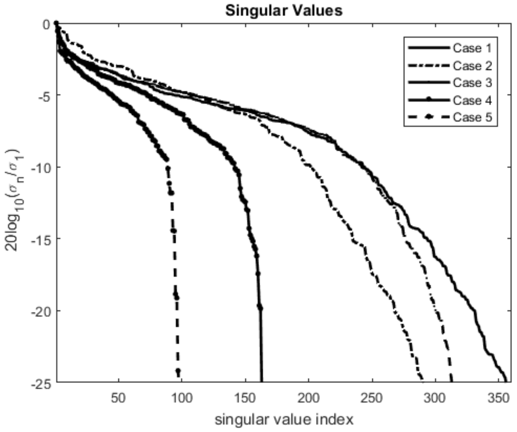
However, the problem arises about the effective location of the measurement points on M and the number of frequencies in . Under the assumption that the measurement domain M and the frequency range are evenly sampled, we consider the five cases summarized in Table 1, which also provides the total amount of collected data, , and the value of TSVD threshold, . This latter is set in correspondence of the beginning of the fast decay of the singular values. For the considered cases, this means to filter out all the singular values whose normalized amplitude is lower than −10 dB, see Figure 2.
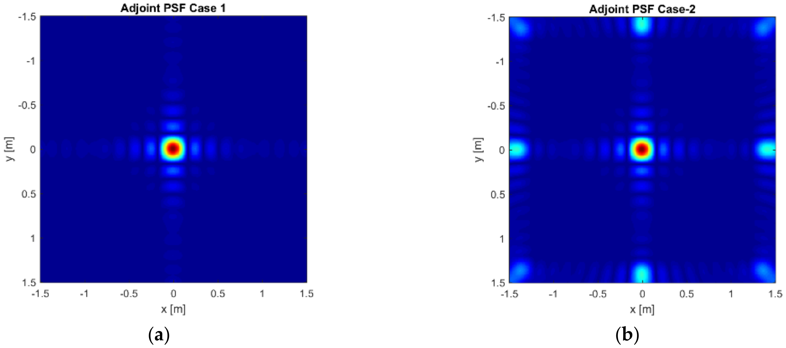
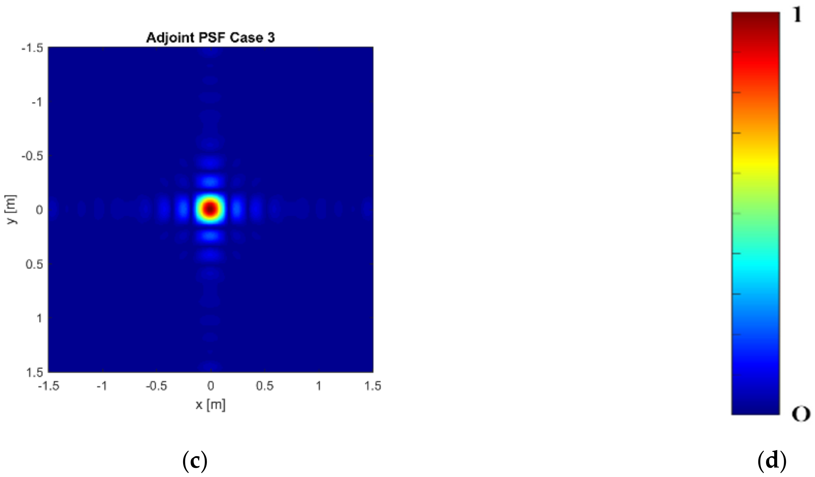
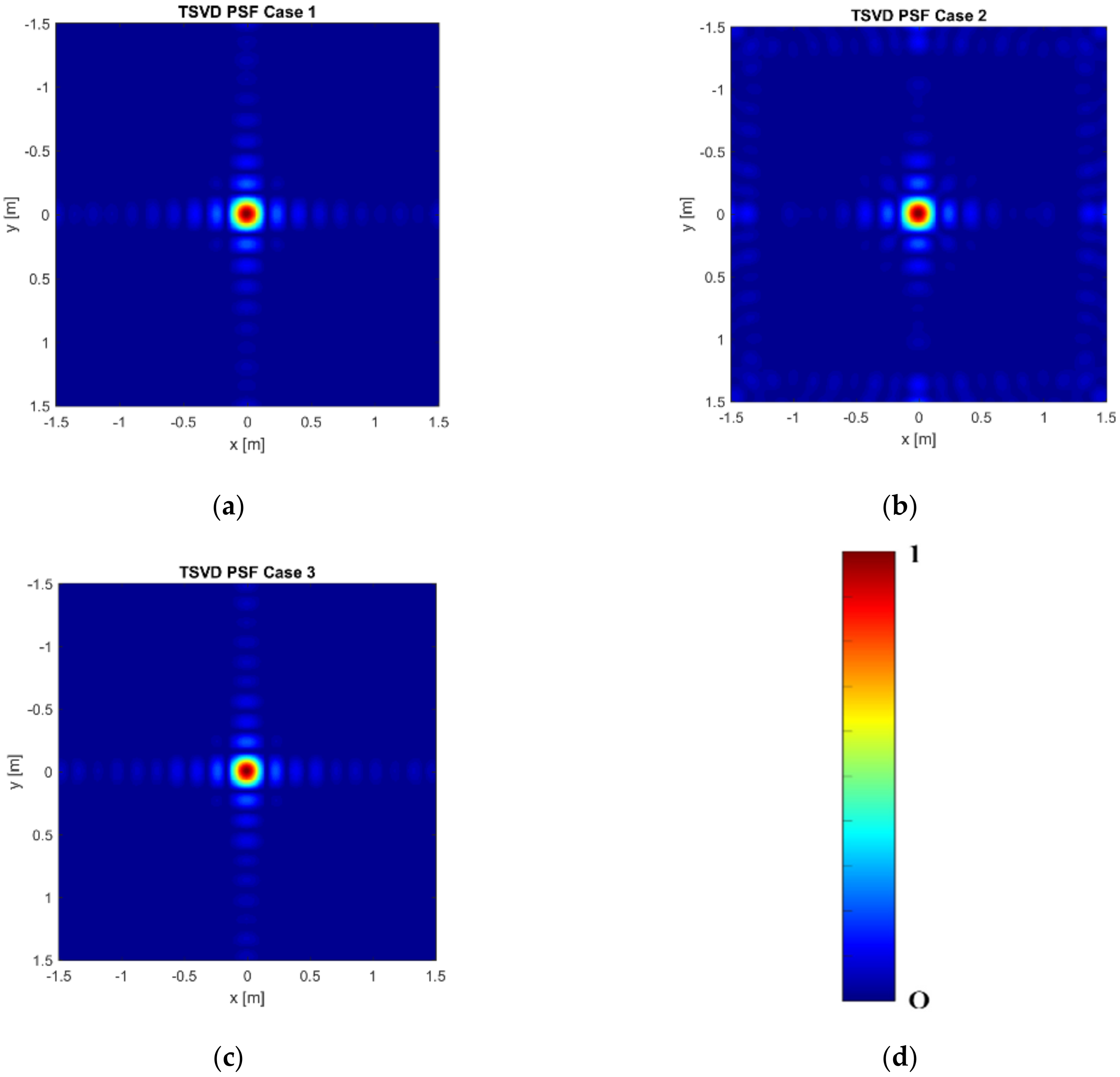
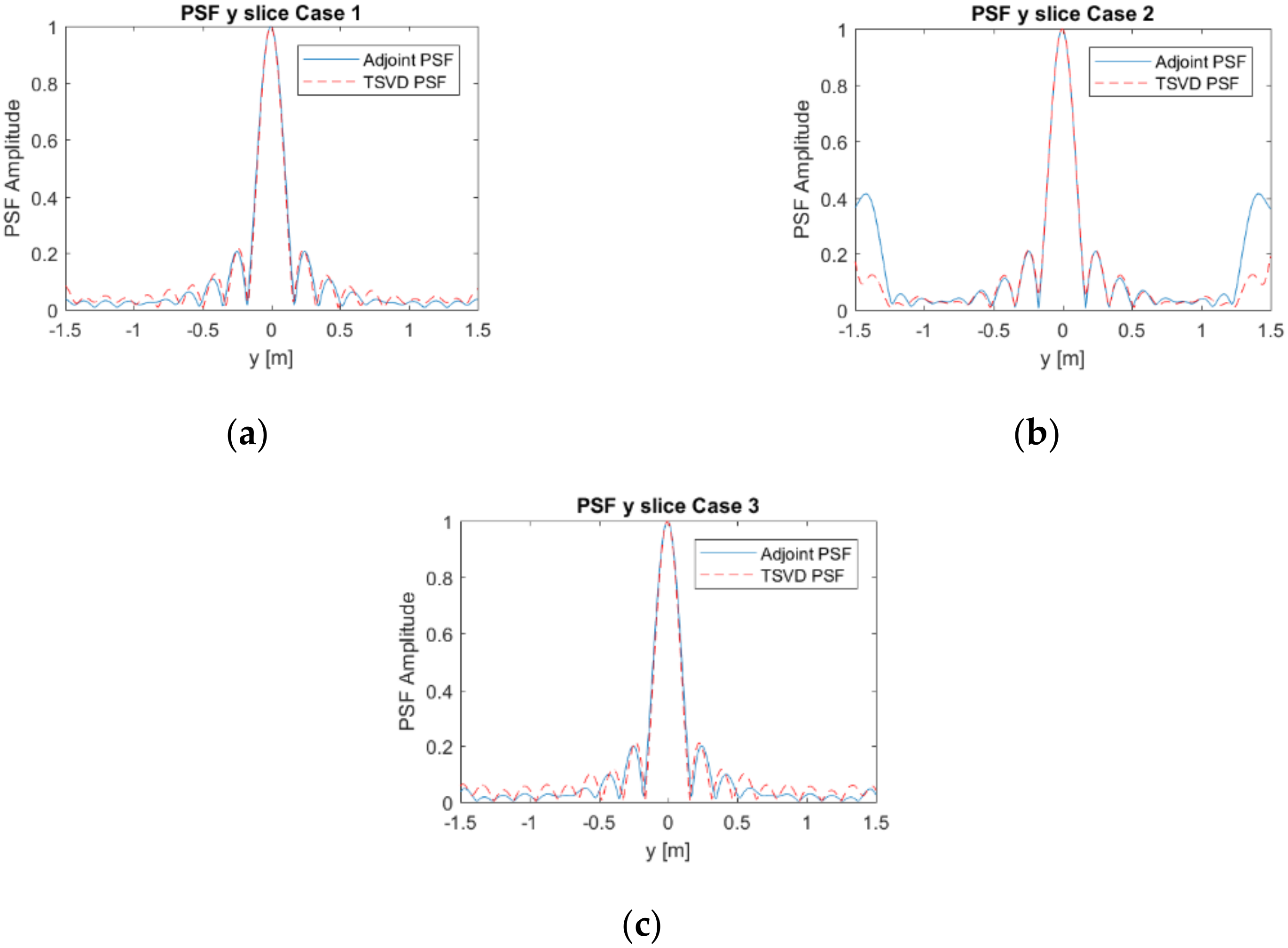
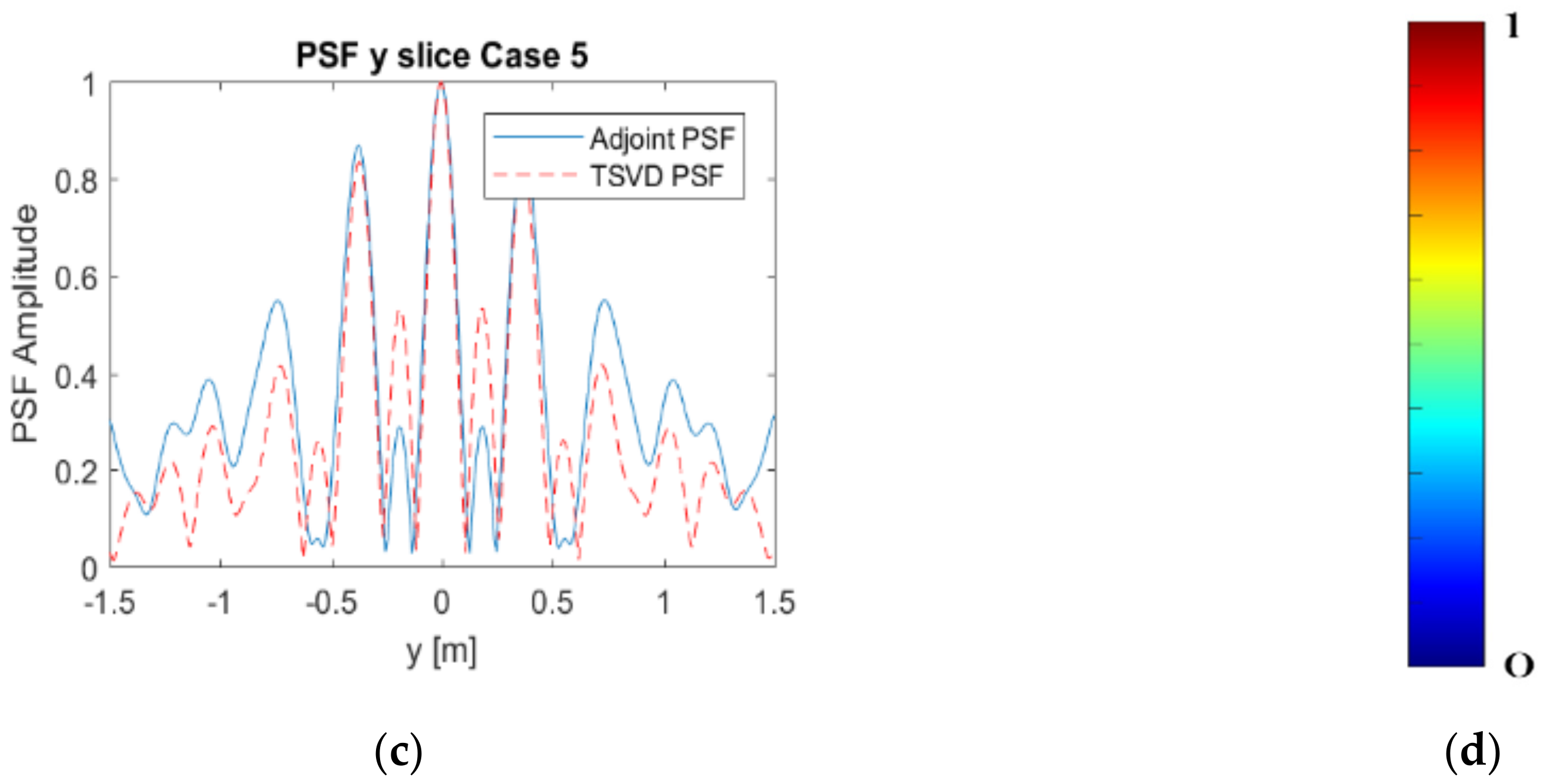
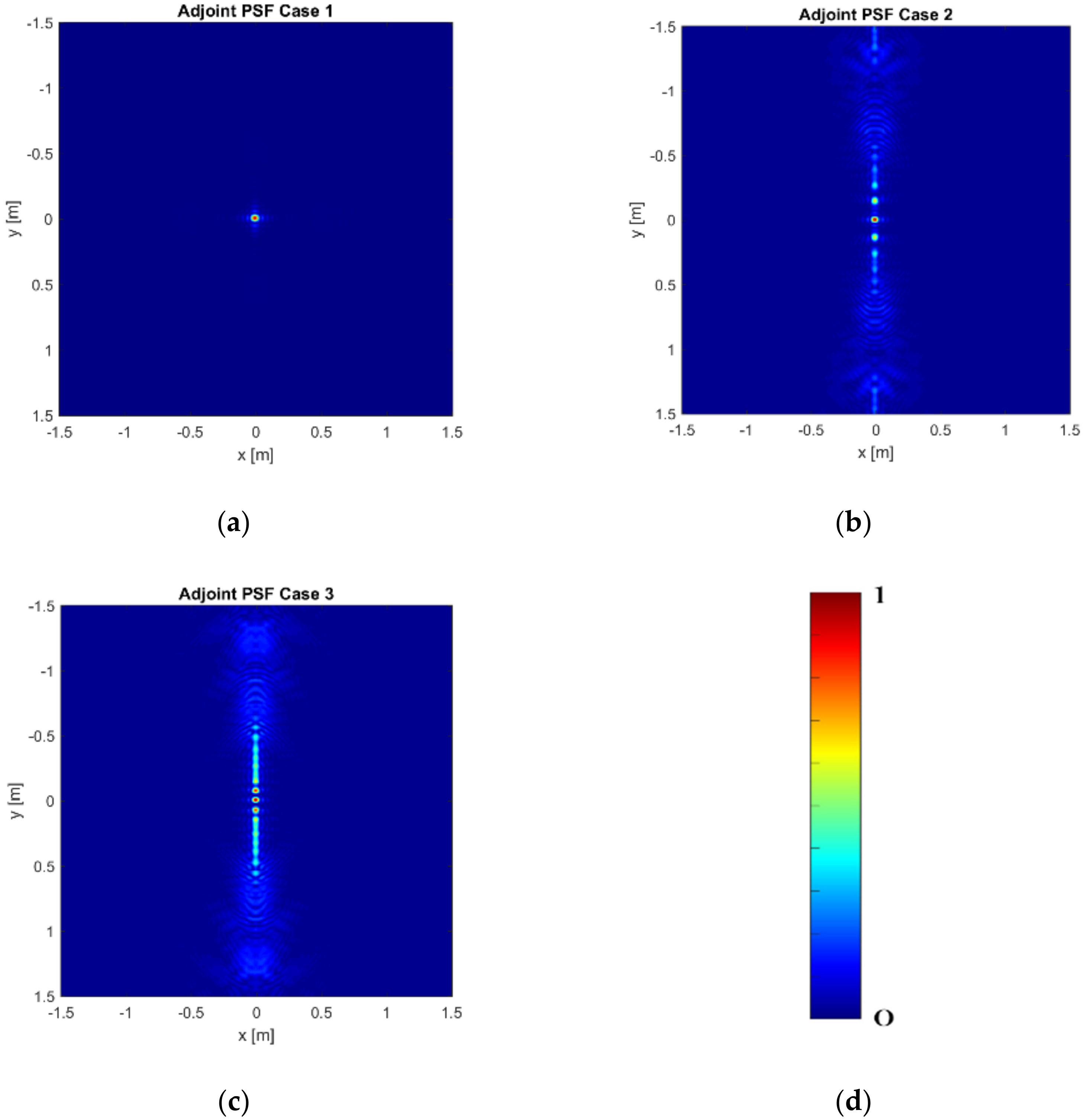
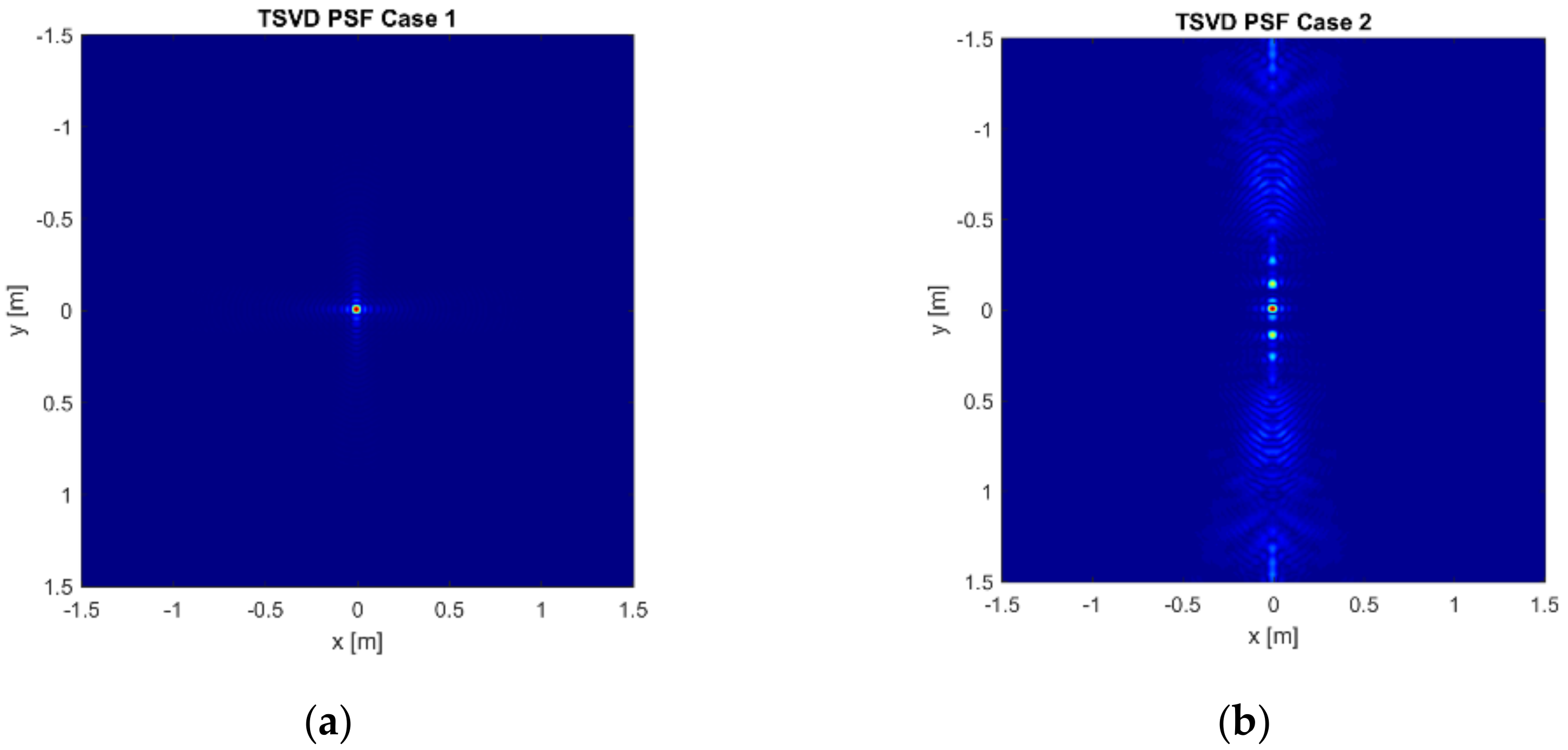
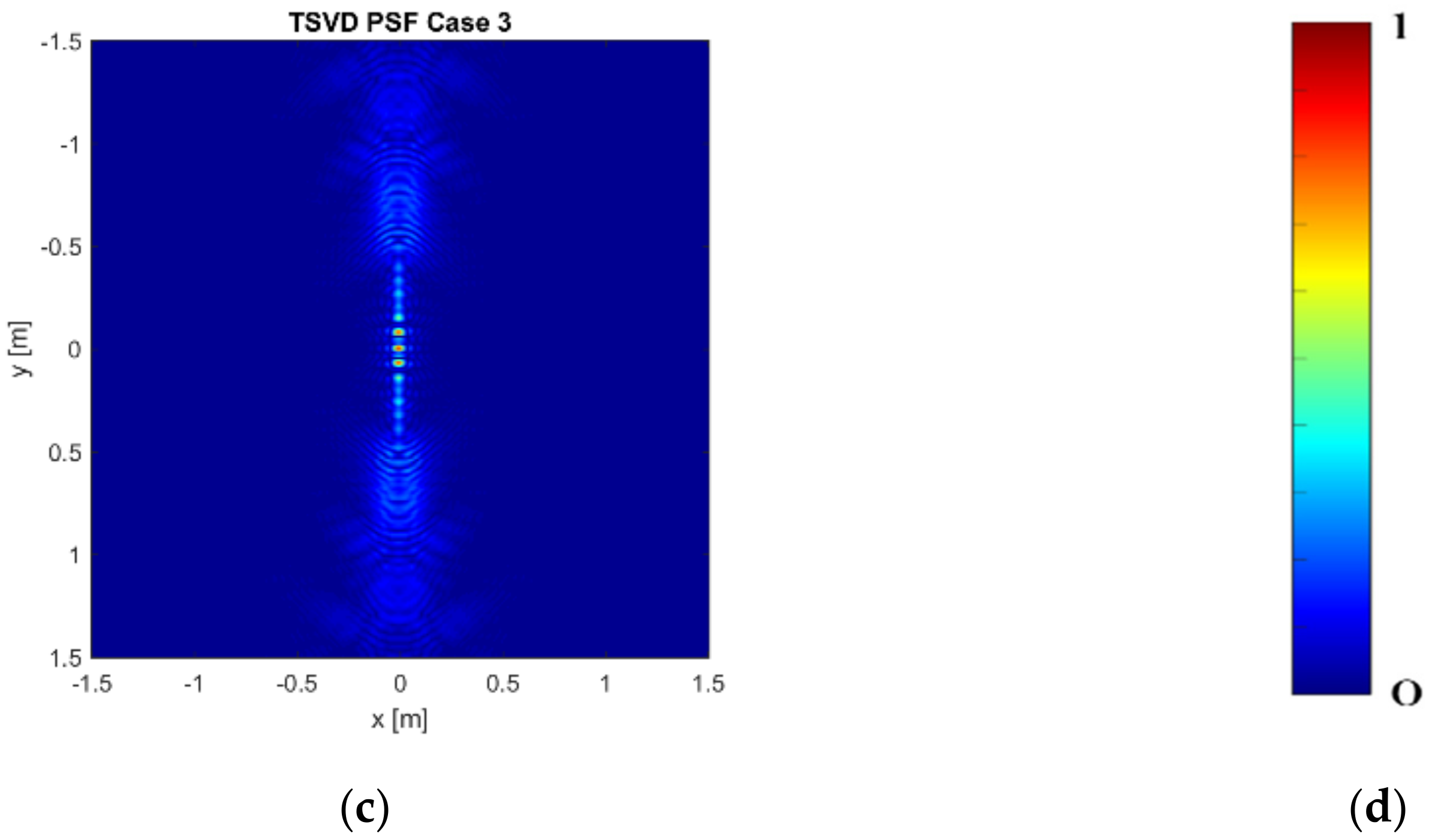
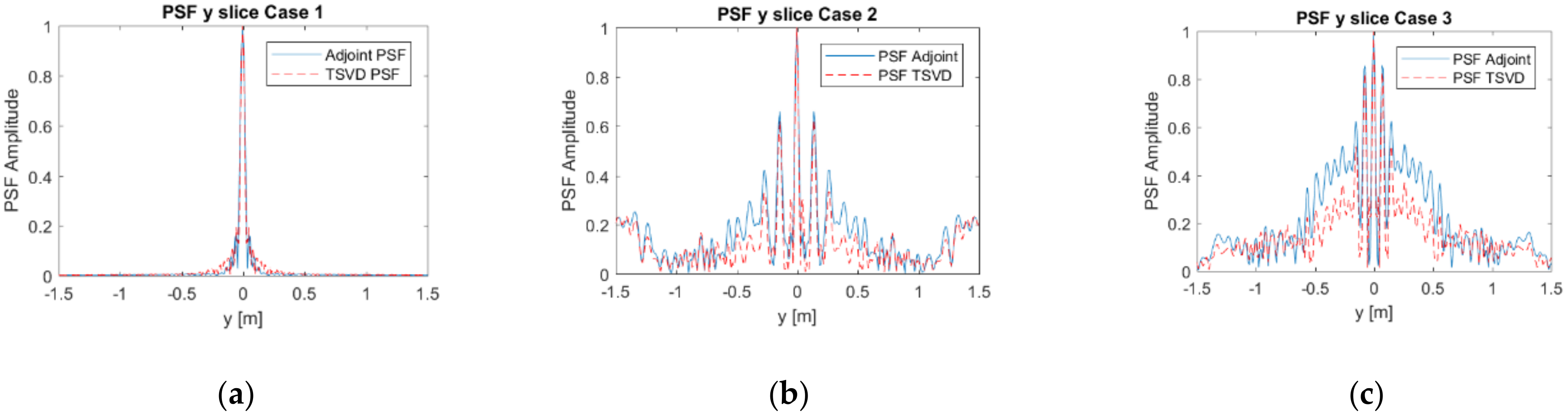
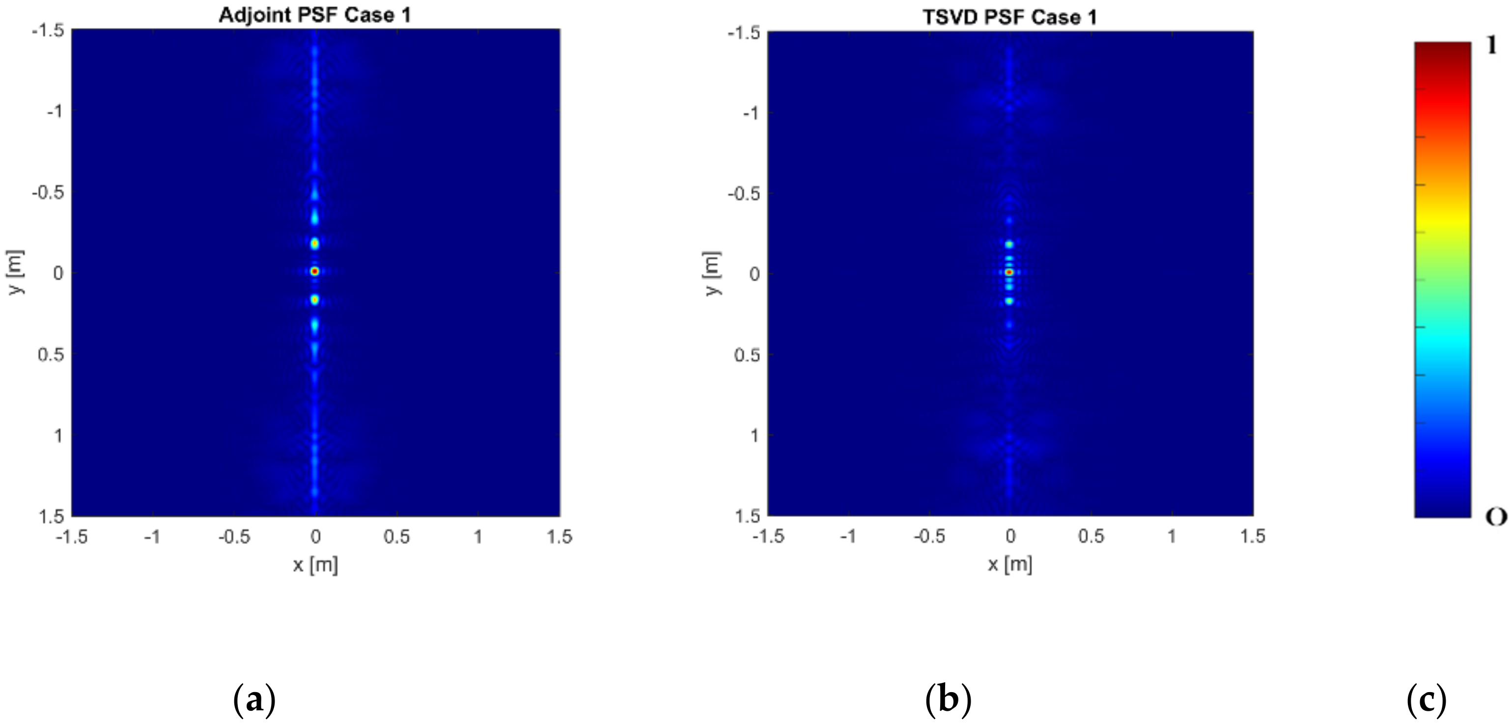
Figure 3a–c and Figure 4a–c show the normalized modulus of the PSF obtained by using Equation (6) (Adjoint PSF) and Equation (7) (TSVD PSF), respectively. In addition, Figure 5a,b compares the PSF cuts along directions. These figures corroborate that both the reconstruction approaches allow for comparable performance in Case 1 and Case 3, while grating lobes occur at the sides of the investigated domain in Case 2, even if they have negligible amplitude for the TSVD approach. Moreover, both the approaches reach a spatial resolution well approximating the expected one. In both the spatial directions, indeed, the spatial resolution achievable by Adjoint and TSVD are 0.18 m and 0.16 m, respectively.
Based on the provided results, we consider Case 3 as the best trade-off in terms of imaging performance and amount of data to be processed. In this case, indeed, both the approaches provide images not affected by grating lobes. Accordingly, it is reasonable of assuming that the measurement parameters of Case 3 allows us to collect the required amount of not redundant data. The other outcome of the present analysis is that, for the example at hand, the number of spatial measurement has a larger effect on the grating lobes issue.
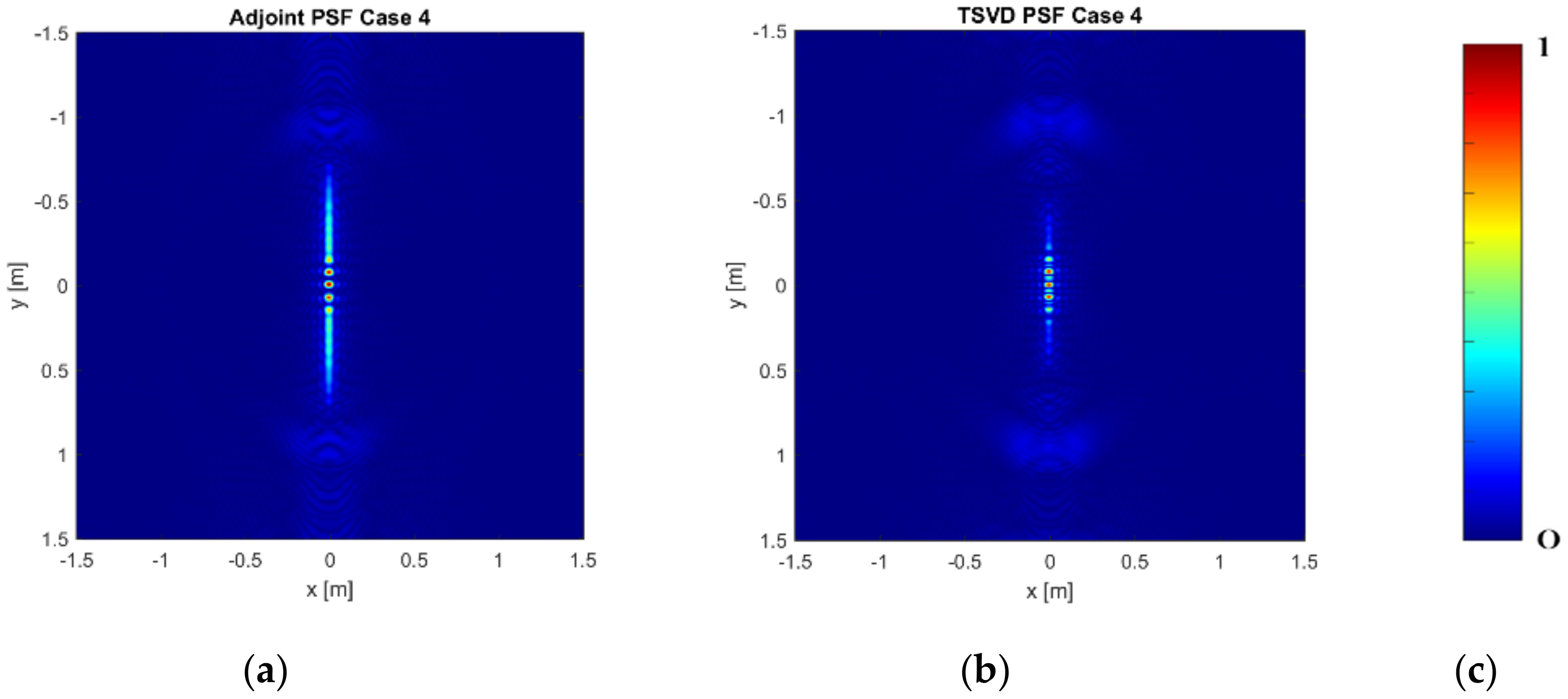
In Case 4 and Case 5, the number of measurement points along x and of frequencies are fixed as in Case 3, while the number of measurement lines along is progressively decreased in order to investigate how the undersampling expected in this direction affects the imaging results.
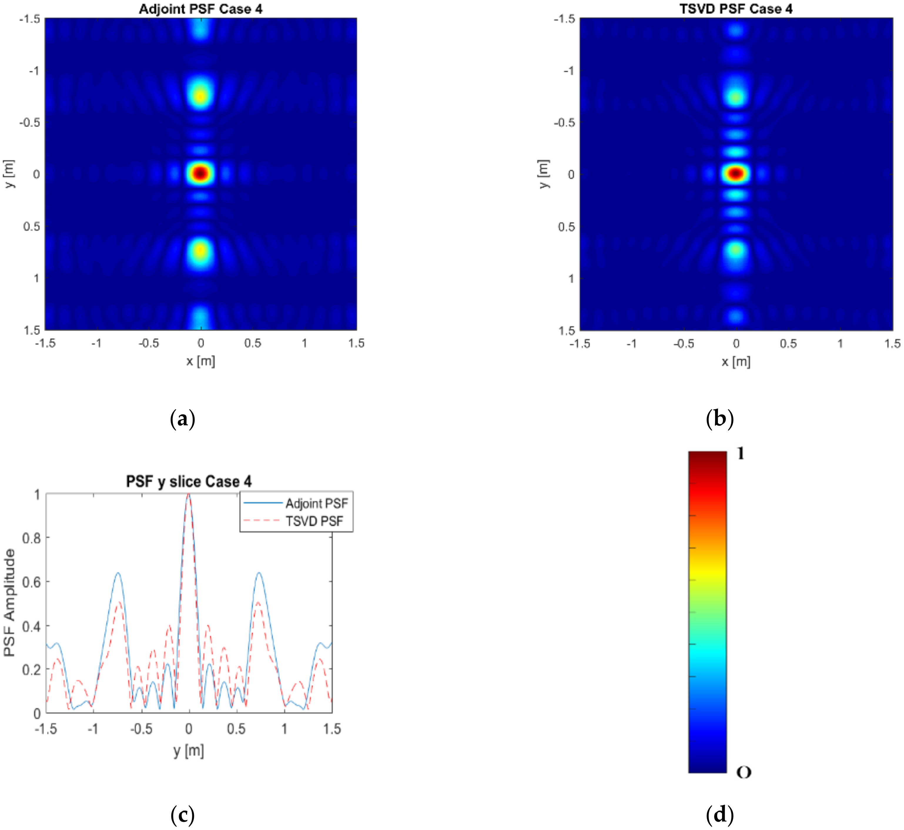
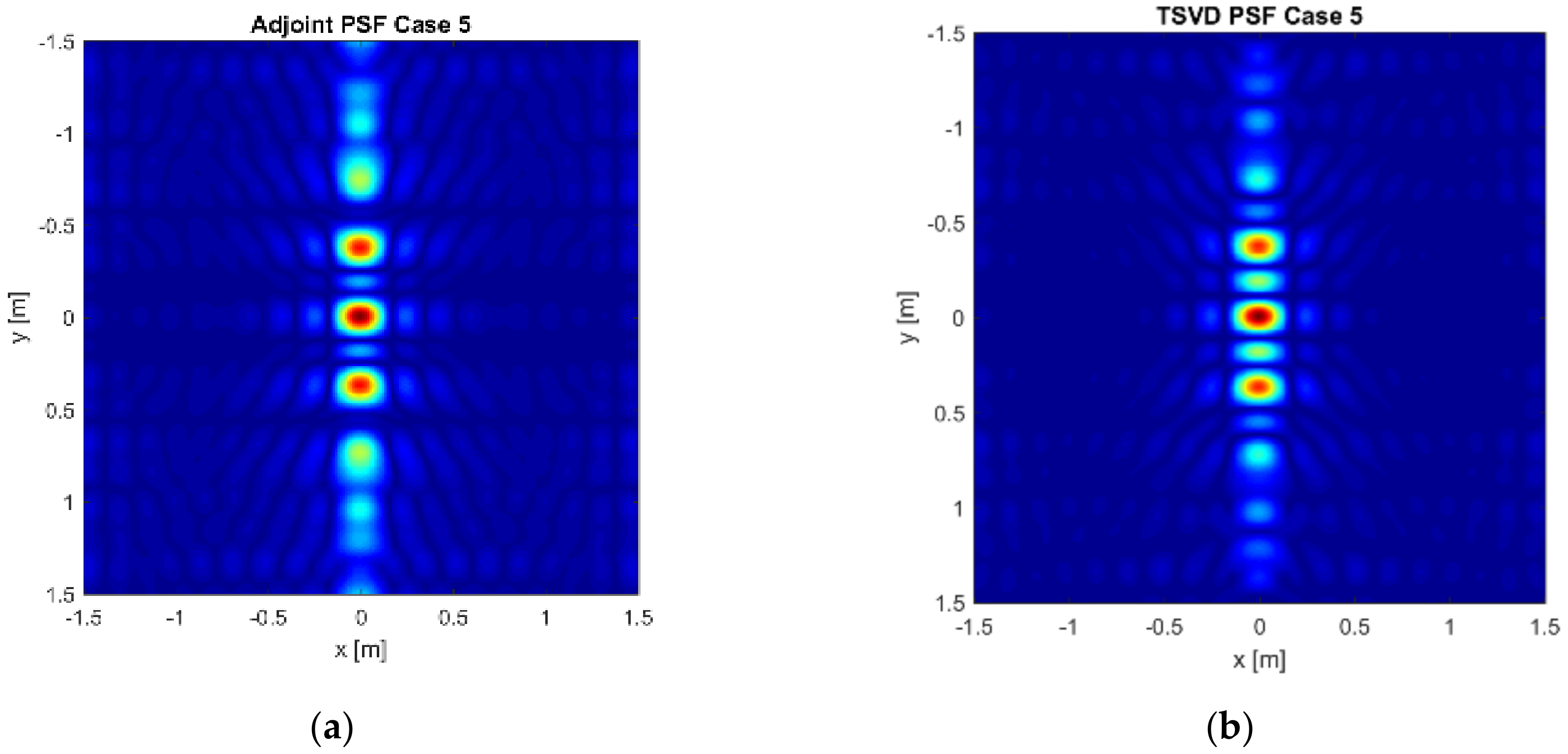
Figure 6a–c is referred to Case 4 while Figure 7a–c accounts for Case 5. As expected, the spatial resolution does not change in both the spatial directions and grating lobes appearing along . Moreover, whatever the inversion procedure, their number increases as the measurement lines decrease, and their location is well approximated by Equation (22) with , being the number of about constant singular values, i.e., the singular values whose normalized amplitude is not less than −6 dB.
Figure 6 and Figure 7 show also that the TSVD inversion allows for improved reconstruction capabilities since the grating lobes have lower amplitude than in the Adjoint reconstruction. This result is compliant with those given in [16,17] and it is due to the not step-like decreasing behaviour of the singular values. It is also worth pointing out that the loss of data, due to reduced number of measurement lines, cannot be compensated for by increasing the number of frequencies. In particular, by setting = 5, the imaging results are similar to those given in Figure 6 and Figure 7 and are not shown for the sake of brevity.
4.2. Example B (Height of the Platform Equal to 2.5 m)
Let us investigate what happens if the assumptions and are removed and assume the flight altitude m. In this case, the PSF analytical expression given in Equation (20) is not valid in principle but, in practice, can be still considered to have indication about the expected performance and to have hints about the design of the measurement configuration. Specifically, in the case at hand, the spatial resolution expected on the basis of the analysis reported in Section 3 is 0.03 m along and , while grating lobes are foreseable when an amount of independent data lower than are gathered.
Based on the previous results, we have considered the cases summarized in Table 2.
Figure 8, Figure 9 and Figure 10 show the 2D PSF reconstructed by means the Adjoint and the TSVD procedures and their cuts along for and . As for the Example A and the following ones, the TVSD threshold has been set in such a way to consider all the singular values before the fast decay. This implies that the threshold is equal to the amount of available data , when few measurement lines are accounted for. Figure 8, Figure 9 and Figure 10 corroborate that, as discussed in Section 3, the spatial resolution improves by decreasing the flight altitude; it does not change when the amount of data decreases, and its value is well estimated by Equation (18). In fact, the spatial resolution is about 0.03 m in both the directions and for both the considered reconstruction approaches. Moreover, as for the flight altitude m, when few measurement lines are considered the TSVD allows for a better reconstruction, in terms of amplitude of grating lobes, compared to the Adjoint procedure, even if the reconstruction provided by both the approaches are affected by artefacts occurring along .
4.3. Example C
Let us consider the reconstruction of a point-like target when the spacing among the measurement lines is fixed and equal to 0.6 m. The target is still located at the center of the investigated domain, which is the same of the previous examples, while the data are collected at the flight altitude m. The measurement points along the x-axis are ; the measurement lines are and , the frequencies in are (see Table 3).
Figure 12a,b show the Adjoint PSF and the TSVD PSF referred to Case 1, while those referred to Case 2 are given in Figure 13a,b.
It is worth noting that the resolutions along are different w.r.t. the previous cases, because the size of the measurement domain along changes. Indeed, for Case 1 the parameter is 1.2 m, while for Case 2 it is m. The resolution values along axis are 0.35 m and 0.7 m for Case 1 and Case 2, respectively; they are compliant with the analytical values given by Equation (18). Moreover, concerning grating lobes, the TSVD approach achieves again better performance w.r.t. the Adjoint inversion procedure. Indeed, Figure 12 and Figure 13 show that the Adjoint PSFs have grating lobes and artefacts whose amplitude is larger compared to the TSVD PSFs.
5. Numerical Example
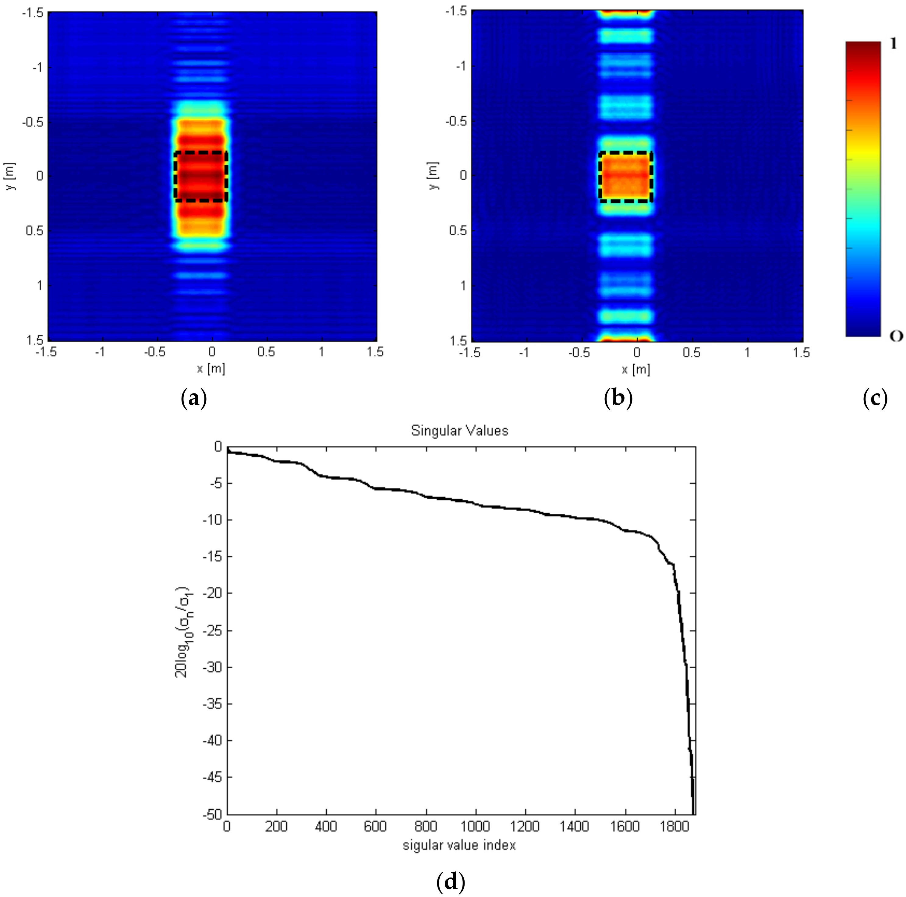
This section aims at assessing the performances of the two reconstruction approaches in the case of extended objects. In particular, we consider an extended object located on a ground having relative permittivity equal to 4. The object is a parallelepiped, having size 0.50 × 0.50 × 0.05 and relative permittivity equal to 6, and it is located about at the center of the investigated domain (the simulated scenario is shown in Figure 14). Specifically, the center of the object is placed at m, m and m.
Time domain data have been simulated by means of gprMax 3D, which is a FDTD simulation software commonly used to simulate time-domain GPR data [18]. Five straight measurement lines are considered along the -axis. They are 3 m long along the x-axis, 0.6 m spaced from m to m, and 2.5 m far from the air-soil interface. A dipole antenna oriented along the -axis, whose central frequency is 4 GHz, is taken as primary source and only the y-component of the backscattered field is collected at evenly spaced measurement points along each line. The simulated data have been transformed into the frequency domain by setting the useful frequency range equal to GHz and considering = 5 frequencies evenly spaced of 0.5 GHz.
Figure 14 shows a sketch of the reference scenario, while Figure 15a,b show Adjoint and TSVD reconstructions in the plane m, where the black dashed contour represents the true target. As for the examples reported in Section 4, the TSVD threshold is such to consider the singular values before the fast decay, i.e., (see Figure 15d). According to the analytical results, the TSVD approach allows for a better spatial resolution and reconstructs accurately shape and size of the object into the plane. On the other hand, few ghosts appear and are due to the grating lobes occurring for the low number of measurement lines. In the TSVD approach, the amplitude of the grating lobes is lower than the amplitude of the object with the exception of those arising on the side of the investigated domain. Conversely, in the Adjoint-based reconstruction, the grating lobes have amplitude comparable to the object and this implies that the -size of the object is significantly overestimated.
6. Discussion and Conclusions
The performance of UAV radar imaging systems depends on multiple system factors, i.e., radar operative parameters, measurement setup and data processing strategy. The paper has presented an analytical and numerical study aimed at assessing the reconstruction capabilities of down looking airborne radar systems able to collect multi-frequency data. The study regards the performance achievable when the imaging is faced under the Born Approximation, which is the usual assumption for facing a radar imaging problem, f.i. in applicative framework of Ground Penetrating Radar [9].
The first part of the presented analysis deals with data collected in far-field condition and satisfying the Nyquist criterion. Under these assumptions, a closed expression of the Point Spread Function (PSF) has been derived and considered as analytical tool to estimate the spatial resolution limits and investigate how the imaging capabilities depend on the amount of available data. It is worth pointing out that the analytical results presented in Section 3 do not depend on the adopted inversion approach and provide a general indication about the achievable imaging capabilities.
In addition, a numerical analysis has been provided to account for the reduced amount of data commonly available, and the far-field condition may not satisfied. The numerical analysis has been carried out by using two widespread inversion strategies, i.e., the Adjoint and the TSVD approaches. Moreover, first, it accounts for a single point-like target and, then, an extended object, whose scattered field has been simulated by using a full-wave electromagnetic software widely exploited by the GPR community. When the measurement configuration is in agreement with the theoretical hypotheses, the numerical results corroborate that the imaging results achieved by means of Adjoint and TSVD inversion approaches exactly match with the resolutions and the grating lobes appearance of the analytical PSF. Conversely, whereas the resolution limits do not change, the occurrence of grating lobes depends on the adopted inversion scheme and the presented results state that the TSVD approach allows for improved results compared to the Adjoint, especially when the flight altitude decreases. Herein, the Adjoint inversion has been considered because it is at the basis of the classical imaging methods (see [10]), while the TSVD inversion was been taken into account due to the fact that the singular values are characterized by a slow dynamic before the fast exponential decay [13]. Other regularization inverse schemes might be used especially when the singular values have a smooth decay [13]; this could be an interesting topic of future work.
As a final remark, we underline that the presented analysis accounts for data collected in ideal conditions, i.e., does not account for the uncertainties about the actual location of the measurement points, which is one of the main problems arising when consider experimental data. Accordingly, the manuscript provides indications about the imaging capabilities achievable by means of a UAV mounted radar system in the best case. As future research activity, we are planning to assemble a radar system on-board a UAV platform, design a measurement campaign in a laboratory-like controlled scenario and exploit the Carrier-phase differential global positioning system (CDGPS) technique [19] to accurately estimate the UAV positions during the data acquisition step. The final goal of this future activity will be the evaluation of the discrepancies between the results achieved by the theoretical analysis and those achieved by processing real datasets.
Author Contributions
Conceptualization, I.C., C.N. and F.S.; Methodology, I.C. and F.S.; Software and Validation, I.C. and C.N.; Formal Analysis, I.C. and C.N.; Investigation, I.C., C.N. and F.S. Data Curation, I.C. and C.N. Writing-Original Draft Preparation, I.C. and C.N.; Supervision, F.S.; Project Administration, I.C. and F.S. All authors have read and agreed to the published version of the manuscript.
Funding
This research received no external funding.
Institutional Review Board Statement
Not applicable.
Informed Consent Statement
Not applicable.
Data Availability Statement
Not applicable.
Conflicts of Interest
The authors declare no conflict of interest.
References
- Li, C.J.; Ling, H. High-resolution, downward-looking radar imaging using a small consumer drone. In Proceedings of the IEEE AP-S Symposium Antennas Propagation, Fajardo, Puerto Rico, 26 June–1 July 2016; pp. 2037–2038. [Google Scholar]
- Colorado, J.; Perez, M.; Mondragon, I.; Mendez, D.; Parra, C.; Devia, C.; Moritz, M.; LNeira, L. An integrated aerial system for landmine detection: SDR-based Ground Penetrating Radar onboard an autonomous drone. Adv. Robot. 2017, 31, 791–808. [Google Scholar] [CrossRef]
- Burr, R.; Schartel, M.; Schmidt, P.; Mayer, W.; Walter, T.; Waldschmidt, C. Design and Implementation of a FMCW GPR for UAV-based Mine Detection. In Proceedings of the IEEE MTT-S International Conference on Microwaves for Intelligent Mobility (ICMIM), IEEE, Munich, Germany, 15–17 April 2018; pp. 1–4. [Google Scholar]
- Eckerstorfer, M.; Jenssen, R.O.R.; Kjellstrup, A.; Storvold, R.; Malnes, E.; Jacobsen, S.K. UAV-Borne UWB Radar for Snowpack Surveys; Technical Report; 2018. [Google Scholar]
- Gonzalez-Diaz, M.; Garcia-Fernandez, M.; Alvarez-Lopez, Y.; Las Heras, F. Improvement of GPR SAR-based techniques for accurate detection and imaging of buried objects. IEEE Trans. Instrum. Meas. 2019, 69, 3126–3138. [Google Scholar] [CrossRef] [Green Version]
- Catapano, I.; Gennarelli, G.; Ludeno, G.; Noviello, C.; Esposito, G.; Renga, A.; Fasano, G.; Soldovieri, F. Small Multicopter-UAV-Based Radar Imaging: Performance Assessment for a Single Flight Track. Remote Sens. 2020, 12, 774. [Google Scholar] [CrossRef] [Green Version]
- Schreiber, E.; Heinzel, A.; Peichl, M.; Engel, M.; Wiesbeck, W. Advanced buried object detection by multichannel, UAV/drone carried synthetic aperture radar. In Proceedings of the 2019 13th IEEE European Conference on Antennas and Propagation (EuCAP), Krakow, Poland, 31 March–5 April 2019; pp. 1–5. [Google Scholar]
- Noviello, C.; Esposito, G.; Catapano, I.; Soldovieri, F. Multilines Imaging Approach for Mini-UAV Radar Imaging System. IEEE Geosci. Remote Sens. Lett. 2021, 1–5. [Google Scholar] [CrossRef]
- Catapano, I.; Gennarelli, G.; Ludeno, G.; Soldovieri, F.; Persico, R. Ground-Penetrating Radar: Operation Principle and Data Processing. Wiley Encycl. Electr. Electron. Eng. 1999, 1–23. [Google Scholar]
- Catapano, I.; Gennarelli, G.; Ludeno, G.; Noviello, C.; Esposito, G.; Soldovieri, F. Contactless Ground Penetrating Radar Imaging: State of the Art, Challenges, and Microwave Tomography-Based Data Processing. IEEE Geosci. Remote Sens. Mag. 2021, 2–24. [Google Scholar] [CrossRef]
- Gennarelli, G.; Catapano, I.; Soldovieri, F. Reconstruction capabilities of down-looking airborne GPRs: The single frequency case. IEEE Trans. Comput. Imaging 2017, 3, 917–927. [Google Scholar] [CrossRef]
- Chew, W.C. Waves and Fields in Inhomogeneous Media; Institute of Electrical and Electronics Engineers: Piscataway, NJ, USA, 1995. [Google Scholar]
- Bertero, M.; Boccacci, P. Introduction to Inverse Problems in Imaging; CRC Press: Boca Raton, FL, USA, 1998. [Google Scholar]
- Schroeder Daniel, J. Astronomical Optics; Elsevier: Amsterdam, The Netherlands, 1999. [Google Scholar]
- Pierri, R.; Persico, R.; Bernini, R. Information content of the Born field scattered by an embedded slab: Multifrequency, multiview, and multifrequency–multiview cases. JOSA A 1999, 16, 2392–2399. [Google Scholar] [CrossRef]
- Pierri, R.; Soldovieri, F. On the information content of the radiated fields in the near zone over bounded domains. Inverse Probl. 1998, 14, 321. [Google Scholar] [CrossRef]
- Fornaro, G.; Serafino, F.; Soldovieri, F. Three-dimensional focusing with multipass SAR data. IEEE Trans. Geosci. Remote. Sens. 2003, 41, 507–517. [Google Scholar] [CrossRef]
- grpMax. Available online: https://www.gprmax.com/ (accessed on 12 February 2021).
- Kaplan, E.; Hegarty, C.J. Understanding GPS-Principles and Applications, 2nd ed.; Artech House: Boston, MA, USA, 2006. [Google Scholar]
Figure 1.
Imaging Scenario.

Figure 2.
Normalized singular values in dB scale (h = 15 m), Case 1—solid line; Case 2—dashed line; Case 3—dashed-dot line; Case 4—circle-solid line; Case 5—circle-dashed line.
Figure 2.
Normalized singular values in dB scale (h = 15 m), Case 1—solid line; Case 2—dashed line; Case 3—dashed-dot line; Case 4—circle-solid line; Case 5—circle-dashed line.

Figure 3.
Normalized modulus of the Adjoint PSF: (a) Case 1— = = 11 and = 5; (b) Case 2— = = 9 and = 5; (c) Case 3— = = 11 and = 3; (d) color bar.
Figure 3.
Normalized modulus of the Adjoint PSF: (a) Case 1— = = 11 and = 5; (b) Case 2— = = 9 and = 5; (c) Case 3— = = 11 and = 3; (d) color bar.


Figure 4.
Normalized modulus of the TSVD PSF: (a) Case 1— = = 11 and = 5; (b) Case 2— = = 9 and = 5; (c) Case 3— = =11 and = 3; (d) color bar.
Figure 4.
Normalized modulus of the TSVD PSF: (a) Case 1— = = 11 and = 5; (b) Case 2— = = 9 and = 5; (c) Case 3— = =11 and = 3; (d) color bar.

Figure 5.
Comparison of Adjoint and TSVD PSF along y: (a) Case 1— = = 11 and = 5; (b) Case 2— = = 9 and = 5; (c) Case 3— = = 11 and = 3.
Figure 5.
Comparison of Adjoint and TSVD PSF along y: (a) Case 1— = = 11 and = 5; (b) Case 2— = = 9 and = 5; (c) Case 3— = = 11 and = 3.

Figure 6.
Normalized modulus of the PSF for = 11, = 5 and = 3: (a) Adjoint PSF (b) TSVD PSF; (c) Comparison of the PSF cuts along y; (d) colorbar.
Figure 6.
Normalized modulus of the PSF for = 11, = 5 and = 3: (a) Adjoint PSF (b) TSVD PSF; (c) Comparison of the PSF cuts along y; (d) colorbar.

Figure 7.
Normalized modulus of the PSF for = 11, = 3 and = 3: (a) Adjoint PSF (b) TSVD PSF; (c) Comparison of the PSF cuts along y; (d) color bar.
Figure 7.
Normalized modulus of the PSF for = 11, = 3 and = 3: (a) Adjoint PSF (b) TSVD PSF; (c) Comparison of the PSF cuts along y; (d) color bar.


Figure 8.
Normalized modulus of the Adjoint PSF: (a) Case 1— = = 63 and = 3; (b) Case 2— = 63 = 5 and = 3; (c) Case 3— = 63 = 3 and = 3; (d) color bar.
Figure 8.
Normalized modulus of the Adjoint PSF: (a) Case 1— = = 63 and = 3; (b) Case 2— = 63 = 5 and = 3; (c) Case 3— = 63 = 3 and = 3; (d) color bar.

Figure 9.
Normalized modulus of the TSVD PSF: (a) Case 1— = = 63 and = 3; (b) Case 2— = 63 = 5 and = 3; (c) Case 3— = 63 = 3 and = 3; (d) color bar.
Figure 9.
Normalized modulus of the TSVD PSF: (a) Case 1— = = 63 and = 3; (b) Case 2— = 63 = 5 and = 3; (c) Case 3— = 63 = 3 and = 3; (d) color bar.


Figure 10.
Comparison of Adjoint and TSVD PSF along y: (a) Case 1— = = 63 and = 3; (b) Case 2— = 63 = 5 and = 3; (c) Case 3— = 63 = 3 and = 3; (d) color bar.
Figure 10.
Comparison of Adjoint and TSVD PSF along y: (a) Case 1— = = 63 and = 3; (b) Case 2— = 63 = 5 and = 3; (c) Case 3— = 63 = 3 and = 3; (d) color bar.

Figure 11.
Normalized modulus of PSF, Case 4: (a) Adjoint procedure, (b) TSVD approach; (c) colorbar.
Figure 11.
Normalized modulus of PSF, Case 4: (a) Adjoint procedure, (b) TSVD approach; (c) colorbar.

Figure 12.
Normalized modulus of PSF, = 63, = 5 and = 5: (a) Adjoint procedure, (b) TSVD approach; (c) color bar.
Figure 12.
Normalized modulus of PSF, = 63, = 5 and = 5: (a) Adjoint procedure, (b) TSVD approach; (c) color bar.

Figure 13.
Normalized modulus of PSF, = 63, = 3 and = 5: (a) Adjoint procedure, (b) TSVD approach; (c) colorbar.
Figure 13.
Normalized modulus of PSF, = 63, = 3 and = 5: (a) Adjoint procedure, (b) TSVD approach; (c) colorbar.

Figure 14.
Simulated Scenario.

Figure 15.
Extended target reconstruction: (a) Adjoint Operator; (b) TSVD (c) colorbar; (d) Normalized singular values. The black dashed contour appearing in Figure 15a,b represents true target at z = 0.
Figure 15.
Extended target reconstruction: (a) Adjoint Operator; (b) TSVD (c) colorbar; (d) Normalized singular values. The black dashed contour appearing in Figure 15a,b represents true target at z = 0.


Table 1.
Parameters for Example A.
| Case | |||||
|---|---|---|---|---|---|
| Case 1 | 11 | 11 | 5 | 605 | 244 |
| Case 2 | 9 | 9 | 5 | 405 | 201 |
| Case 3 | 11 | 11 | 3 | 363 | 241 |
| Case 4 | 11 | 5 | 3 | 165 | 141 |
| Case 5 | 11 | 3 | 3 | 99 | 88 |
Table 2.
Parameters for Example B.
| Case | |||||
|---|---|---|---|---|---|
| Case 1 | 63 | 63 | 3 | 11,907 | 6549 |
| Case 2 | 63 | 5 | 3 | 945 | 945 |
| Case 3 | 63 | 3 | 3 | 567 | 567 |
| Case 4 | 63 | 3 | 5 | 945 | 945 |
Table 3.
Parameters for Example 3.
| Case | T | ||||
|---|---|---|---|---|---|
| Case 1 | 63 | 5 | 5 | 1575 | 1575 |
| Case 2 | 63 | 3 | 5 | 945 | 945 |
Publisher’s Note: MDPI stays neutral with regard to jurisdictional claims in published maps and institutional affiliations. |
© 2021 by the authors. Licensee MDPI, Basel, Switzerland. This article is an open access article distributed under the terms and conditions of the Creative Commons Attribution (CC BY) license (https://creativecommons.org/licenses/by/4.0/).
Share and Cite
MDPI and ACS Style
Catapano, I.; Noviello, C.; Soldovieri, F. Down-Looking Airborne Radar Imaging Performance: The Multi-Line and Multi-Frequency. Remote Sens. 2021, 13, 4897. https://0-doi-org.brum.beds.ac.uk/10.3390/rs13234897
AMA Style
Catapano I, Noviello C, Soldovieri F. Down-Looking Airborne Radar Imaging Performance: The Multi-Line and Multi-Frequency. Remote Sensing. 2021; 13(23):4897. https://0-doi-org.brum.beds.ac.uk/10.3390/rs13234897
Chicago/Turabian StyleCatapano, Ilaria, Carlo Noviello, and Francesco Soldovieri. 2021. "Down-Looking Airborne Radar Imaging Performance: The Multi-Line and Multi-Frequency" Remote Sensing 13, no. 23: 4897. https://0-doi-org.brum.beds.ac.uk/10.3390/rs13234897
Note that from the first issue of 2016, this journal uses article numbers instead of page numbers. See further details here.