
Driving Forces of the Changes in Vegetation Phenology in the Qinghai–Tibet Plateau

1
State Key Laboratory of Desert and Oasis Ecology, Xinjiang Institute of Ecology and Geography, Chinese Academy of Sciences, Urumqi 830011, China
2
University of Chinese Academy of Sciences, Beijing 100049, China
3
School of Geography Science and Tourism, Xinjiang Normal University, Urumqi 830054, China
*
Author to whom correspondence should be addressed.
Remote Sens. 2021, 13(23), 4952; https://0-doi-org.brum.beds.ac.uk/10.3390/rs13234952
Submission received: 24 September 2021
/
Revised: 22 November 2021
/
Accepted: 2 December 2021
/
Published: 6 December 2021
Abstract
:Phenological change is an emerging hot topic in ecology and climate change research. Existing phenological studies in the Qinghai–Tibet Plateau (QTP) have focused on overall changes, while ignoring the different characteristics of changes in different regions. Here, we use the Global Inventory Modeling and Mapping Studies (GIMMS3g) normalized difference vegetation index (NDVI) dataset as a basis to discuss the temporal and spatial changes in vegetation phenology in the Qinghai–Tibet Plateau from 1982 to 2015. We also analyze the response mechanisms of pre-season climate factor and vegetation phenology and reveal the driving forces of the changes in vegetation phenology. The results show that: (1) the start of the growing season (SOS) and the length of the growing season (LOS) in the QTP fluctuate greatly year by year; (2) in the study area, the change in pre-season precipitation significantly affects the SOS in the northeast (p < 0.05), while, the delay in the end of the growing season (EOS) in the northeast is determined by pre-season air temperature and precipitation; (3) pre-season precipitation in April or May is the main driving force of the SOS of different vegetation, while air temperature and precipitation in the pre-season jointly affect the EOS of different vegetation. The differences in and the diversity of vegetation types together lead to complex changes in vegetation phenology across different regions within the QTP. Therefore, addressing the characteristics and impacts of changes in vegetation phenology across different regions plays an important role in ecological protection in this region.
1. Introduction
Vegetation is an important aspect of surface material composition. Vegetation plays a crucial role in regulating the biosphere and the atmosphere by affecting carbon absorption, the hydrological cycle, and energy exchange in the ecosystem. Phenology, which mainly studies the periodicity of biological cycles affected by climate change, provides an independent measure of how ecosystems respond to these changes [1,2]. Most scholars agree that climate change has a significant impact on terrestrial ecosystems [3,4,5,6,7], regulating regional and global climate through geo-biochemical and biophysical feedback [8,9].
Further, vegetation phenology refers to the corresponding changes in vegetation rhythms when environmental conditions vary periodically [10]. Hence, vegetation phenology better reflects the dynamic response relationship between vegetation ecosystems and climate change [3,11]. Leaf emergence and senescence are important stages in vegetation growth and play a critical role in carbon absorption in vegetation ecosystems [12,13]. In addition, changes in vegetation phenology also affect the interaction between different species and nutrition, impacting the composition of species community [14]. Therefore, studies on the response relationship between vegetation phenology and climate change have increased in number in recent decades. Spring vegetation phenology has remained the focus of most recent studies, as total carbon absorption of vegetation in a year is mainly limited by field observation and regional remote sensing methods [15,16,17,18]. These approaches are mostly used to study the response relationship between vegetation phenology and air temperature in spring [19,20]. However, some studies have shown that the extension of the growing season is mainly driven by the delay in autumn phenology in the temperate zone of the northern hemisphere regions [21,22]. Autumn phenology thus assumes a key position in regulating the nitrogen cycle, ecosystem function, and interaction with the climate system [14]. Therefore, the feedback mechanism between vegetation phenology and climate change can be clarified systematically through an in-depth inquiry into the changes in vegetation phenology in spring and autumn.
The unique climatic conditions of the Qinghai–Tibet Plateau (QTP) strongly impact the carbon cycle of the regional ecosystem. Previous studies have shown that climate warming in the plateau has led to significant changes in the ecological environment, such as the increase in primary productivity and the advance of vegetation phenology in spring. Studies on the phenology of the vegetation growing season in the study region have focused on the analysis of the response relationship between its spatiotemporal trend and climate change [23,24,25]. Nonetheless, most previous studies aimed at exploring the response mechanism between vegetation phenology and rising air temperature [26,27], ignoring the role of precipitation drivers. However, precipitation is an important factor affecting the start and the end of the vegetation growing season [28], especially in dry climate areas [29], and detailed analysis of the feedback between vegetation phenology and different periods (months) of temperature and precipitation before the growing season is still rare.
In addition, there is an obvious spatial heterogeneity among the vegetation components in the QTP, which leads to enormous differences in the response relationship between vegetation phenology and climatic factors affecting the different vegetation types [25]. Consequently, it is necessary to systematically study the response and feedback mechanisms between vegetation phenology and temperature and precipitation in the pre-season, so as to deepen our understanding of how climate change affects vegetation phenology in the study area. However, due to limitations in using ground observation to study vegetation phenology in the QTP, a remote sensing approach holds greater promise for spatial vegetation monitoring purposes [24,30]. As such, this study uses the Global Inventory Modeling and Mapping Studies (GIMMS3g) normalized difference vegetation index (NDVI) dataset from 1982 to 2015 to extract vegetation phenology for different years in this region. This dataset has been corrected to minimize various errors and noises resulting from calibration, orbital drift, viewing geometry, stratospheric volcanic aerosols, and other factors unrelated to vegetation dynamics [31]. This dataset has been widely employed in research work involving long time series of changes in vegetation dynamics [24,28,30]. Additionally, this dataset will be used to study the characteristics and trends in vegetation phenology in the plateau in the months leading up to the growing season, along with the main driving forces affecting the phenology of the different vegetation types.
In this paper, we use the GIMMS3g dataset to extract the start of the growing season (SOS), the end of the growing season (EOS), and the length of the growing season (LOS) for vegetation, and systematically analyze the characteristics of the changes in vegetation phenology and the response relationship between vegetation phenology and climatic factors across the study area. The main objectives of this study were to: (1) investigate the characteristics of the spatial and temporal changes in vegetation phenology in the QTP during the period 1982–2015; (2) evaluate the effects of pre-season temperature and precipitation on the SOS and the EOS in different areas of the study area; (3) explore the feedback mechanism between vegetation phenology and climatic factors in the study area. The study findings enable predicting the future evolution of ecosystems and implementing effective ecosystem management.
2. Material and Methods
In this section, we describe the materials and methods used in this study. First, we describe the general situation in the study area, then elaborate on data acquisition and data processing, and finally all of the analyze the results.
2.1. Study Area
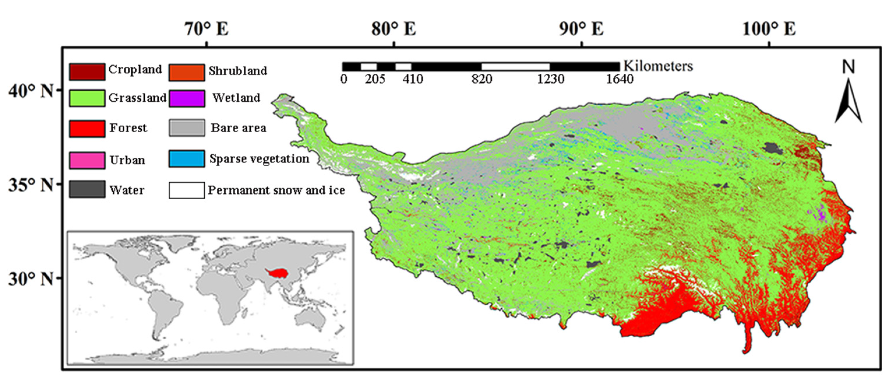
The QTP is one of the most elevated regions on Earth, with a mean elevation of ~4000 m above sea level, and is consequently known as “the roof of the world”, with a geographical range of 26°0′0″N–39°47′N to 73°19′ E–104°47′E (Figure 1), covering an area of ~3 × 10⁶ km2 [32]. The QTP and its surrounding mountains are also known as “The Water Tower of Asia” [33], as the source of several major Asian rivers such as the Yellow River, the Yangtze, Indus, Ganges, Brahmaputra, Irrawaddy, Salween and Mekong, and provide water to more than one billion people living downstream [34]. The population in this region is small and its density is low, with an average of 4.05 people/km2, far lower than the national average population density of 119 people/km2 [35]. Due to the impact of topographical factors, the QTP has formed a unique climate. The QTP is characterized by a low temperature, low humidity, low cloud cover, and abundant sunshine. The annual mean, the minimum and the maximum air temperature between 1980 and 2018 obtained from the 95 China Meteorological Administration (CMA) (http://data.cma.cn/en, accessed on 12 October 2020) weather stations in the QTP are 4.1, 2.8, and 5.1 °C, respectively [32]. Due to global warming, the temperature in this region has increased significantly and was 2-fold higher than the rate of global warming (0.014 °C/a) during the period 1961–2015 [32]. Further, the spatial heterogeneity of precipitation across the QTP is apparent [36], with an annual mean, minimum and maximum precipitation of 482, 418, and 553 mm in the period 1980–2018 from the 95 CMA weather stations in the QTP, respectively [32]. For example, annual summer precipitation decreases gradually from the southeast (~700 mm) to the northeast (~50 mm) [36]. Grassland is the dominant vegetation type in this region (Figure 1). In order to study the driving forces of vegetation phenology in the study area, we choose only pixels that have the same class between 1992 and 2015 by using yearly land -cover data from the European Space Agency (ESA) climate change initiative (CCI) [37]. The land -cover data have a spatial resolution of 300 m and are divided into 37 categories, which are finally merged into ten categories (cropland, grassland, forest, urban, water, shrubland, wetland, bare area, sparse vegetation, and permanent snow and ice) in this study. Nevertheless, we selected only land cover types (cropland, grassland, forest, shrubland, and spare vegetation) that remained unchanged from 1992 to 2015 for the different vegetation types.
2.2. Data Acquisition
The GIMMS3g NDVI dataset is used to study the longtime range. The time range of the dataset in the present study is from 1982 to 2015, with a spatial resolution of approximately 8 km and is updated every half month. Additionally, the Digital Elevation Model at a spatial resolution of 1 km was utilized to record the changes in vegetation phenology at different elevations. The Digital Elevation Model was developed at the Resource and Environmental Science and Data Center of the Chinese Academy of Sciences. Furthermore, the Long-Term Snow Depth Product for China (LSDPC), with a spatial resolution of 0.25°, provided by the Cold and Arid Regions Sciences Data Center in Lanzhou during the period 1979–2015, was used; it is updated once a month. Daily temperature from 1982 to 2015 recorded at meteorological stations across the QTP was provided by the China Meteorological Data Sharing System (http://cdc.nmic.cn/home.do, accessed on 12 November 2020).
Further, to evaluate the interaction between vegetation phenology and climatic factors, we relied on air temperature (°C) and precipitation (mm) data retrieved from the CRUTSv.4.04 grid data released by the British Atmospheric Data Center (http://badc.nerc.ac.uk/data/cru/, accessed on 12 November 2020). Air temperature and precipitation represent the monthly average and monthly sum for air temperature and precipitation, respectively. The time series of this dataset is 1901 to 2019, with a spatial resolution of 0.5°, and it is updated once a month.
2.3. Data Processing
In this section, we elaborate on the data processing used in this study. First, we describe the method used for vegetation phenology extraction in detail and then introduce the method used for meteorological data extraction.
2.3.1. Extraction of Data on Vegetation Phenology
Snow cover in the non-growing season often distorts NDVI values, which leads to errors in phenological retrieval [38]. In our research, we used daily air temperature (below 0 °C for 5 consecutive days) to identify the pixels most likely contaminated by snow and replaced those with the nearest uncontaminated winter NDVI values [29]. This method has been verified in a previous report [39]. A smooth curve was then fitted using the Savitzky Golay filter from the time series of NDVI data [40]. A dynamic threshold method has been employed to retrieve the vegetation phenological parameters [41]. Further, dynamic thresholds defined as NDVI ratios of 20% were used to determine the SOS [42,43]. Specifically, the SOS is defined as the first day of the year when the NDVI ratio value exceeds 0.2. The NDVI ratio is described in Equation (1):
NDVIratio = (NDVIt − NDVImin)/(NDVImax − NDVImin)
Here, NDVIt is the NDVI at time t; NDVImax and NDVImin stand for the maximum and the minimum NDVI values in the annual NDVI time series, respectively. Additionally, a threshold of 60% was originally employed to determine the EOS by Yu et al. from in situ observations in the QTP [44]. To eliminate the impact of sparse vegetation and bare soil on the NDVI, we extracted pixels with an average annual NDVI (1982–2015) greater than 0.1 [30]. Additionally, the extraction of the above parameters was mainly completed in TIMESAT3.3.
2.3.2. Meteorological Data Processing
For temperature, precipitation and snow depth changes, we calculated the monthly and annual averages from 1982 to 2015 using the corresponding datasets. To study the relationship between climatic factors (air temperature and precipitation) and vegetation phenology from 1982 to 2015, we unified the spatial resolution of climatic factor grid data with vegetation phenology using the proximity method in Matlab2016a; hence, the consistency in spatial resolution. However, given the inconsistency between vegetation phenology and the distribution of the target data (air temperature and precipitation), we used the annual vegetation phenology distribution as a template to mask out the grid data to ensure one-to-one correspondence between vegetation phenology and climatic factors.
We then selected the spatial response relationship between pre-season air temperature and precipitation and the SOS from 1982 to 2015, respectively. Further, we selected the spatial response relationship between pre-season air temperature, precipitation and the EOS from 1982 to 2015, respectively. The above experimental processes were performed in Matlab2016a.
2.4. Analyses
The SOS, the EOS, and the LOS for each pixel in the QTP were calculated using the GIMMS3g NDVI datasets. To calculate the interannual trend in the SOS, the EOS, and the LOS of the study area, a simple linear regression method was used to analyze the interannual trend in each pixel. To detect the trend turning points in the SOS, the EOS, and the LOS at the regional scale, we applied the Mann–Kendall (MK) method test, which is a non-parametric significance test, to statistically assess whether there is a monotonic upward or downward trend in a variable overtime [45]. Here, this test has been applied to multiple trend analyses of NDVI data [26]. In our study, a significance level of 0.05 was used. To evaluate the response of the SOS and the EOS to climatic change in different regions during the pre-season, we applied a temporal partial correlation analysis to the SOS, the EOS, pre-season air temperature, and precipitation for all pixels of the different regions in the QTP [28].
Random forest regression tree analysis is an extension of the decision tree algorithm for continuous response variables [46]. This was employed to determine the most important climatic factors driving vegetation phenology. Random forest regression tree analysis can also be used to describe the interaction between climatic factors and vegetation [47]. Regarding the degree of phenology driven by climatic factors affecting the different vegetation types, our analysis is completed by using the random forest software package in R [48]. We selected air temperature and precipitation in the pre-season as the driving forces of the changes in vegetation phenology. Relevant scholars have found that feedback between temperature, precipitation, and vegetation phenology is at its greatest in the first month of the pre-season [24,28]. According to the annual average change in the SOS and the EOS, the SOS in the study area is mainly in April, May, and June, while the EOS is mainly in August, September, and October. So, we discussed the driving forces air temperature and precipitation in the first month of the pre-season and the SOS, the EOS of every pixel for the different vegetation types.
Accordingly, we carried out the regression of 500 trees in each of the six vegetation communities in the study area. The regression trees were tested using air temperature and precipitation in March, April, and May and the growing season of the different vegetation types. Further, the regression trees were tested using air temperature and precipitation in August, September and October at the EOS.
As such, we found the random forest model to be useful for addressing the following key research questions: (1) What is the comprehensive impact of air temperature and precipitation on the SOS and the EOS of the different vegetation types in the study area? (2) Among factors such as air temperature and precipitation in different months, what are the most important factors driving the phenology of the different vegetation types at the SOS and the EOS?
3. Results
In this section, we mainly analyze the characteristics of the changes in vegetation phenology, and the response relationship between vegetation phenology and climatic factors in the study area.
3.1. Characteristics of the Changes in Vegetation Phenology in the Qinghai–Tibet Plateau
In this section, first, we analyze the characteristics of the temporal changes in vegetation phenology, and then analyze the characteristics of the spatial changes in vegetation phenology.
3.1.1. Characteristics of the Temporal Changes in Vegetation Phenology
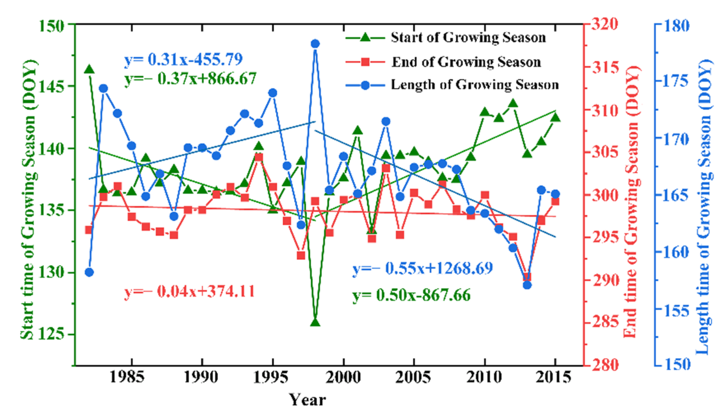
By analyzing the characteristics of the interannual changes in the SOS, the EOS and the LOS of the vegetation phenology in the QTP from 1982 to 2015 (Figure 2), we found that all of these fluctuations of different ranges. For instance, the EOS is 0.40 day/decade ahead of schedule, which is only a slight change. However, both the SOS and the LOS show significant changes between 1982 and 1998, advancing 3.70 and 3.10 days/decade, respectively. Similarly, from 1998 to 2015, the SOS and the LOS were delayed by 5.0 and 5.5 days/decade, respectively.
3.1.2. Characteristics of the Spatial Changes in Vegetation Phenology
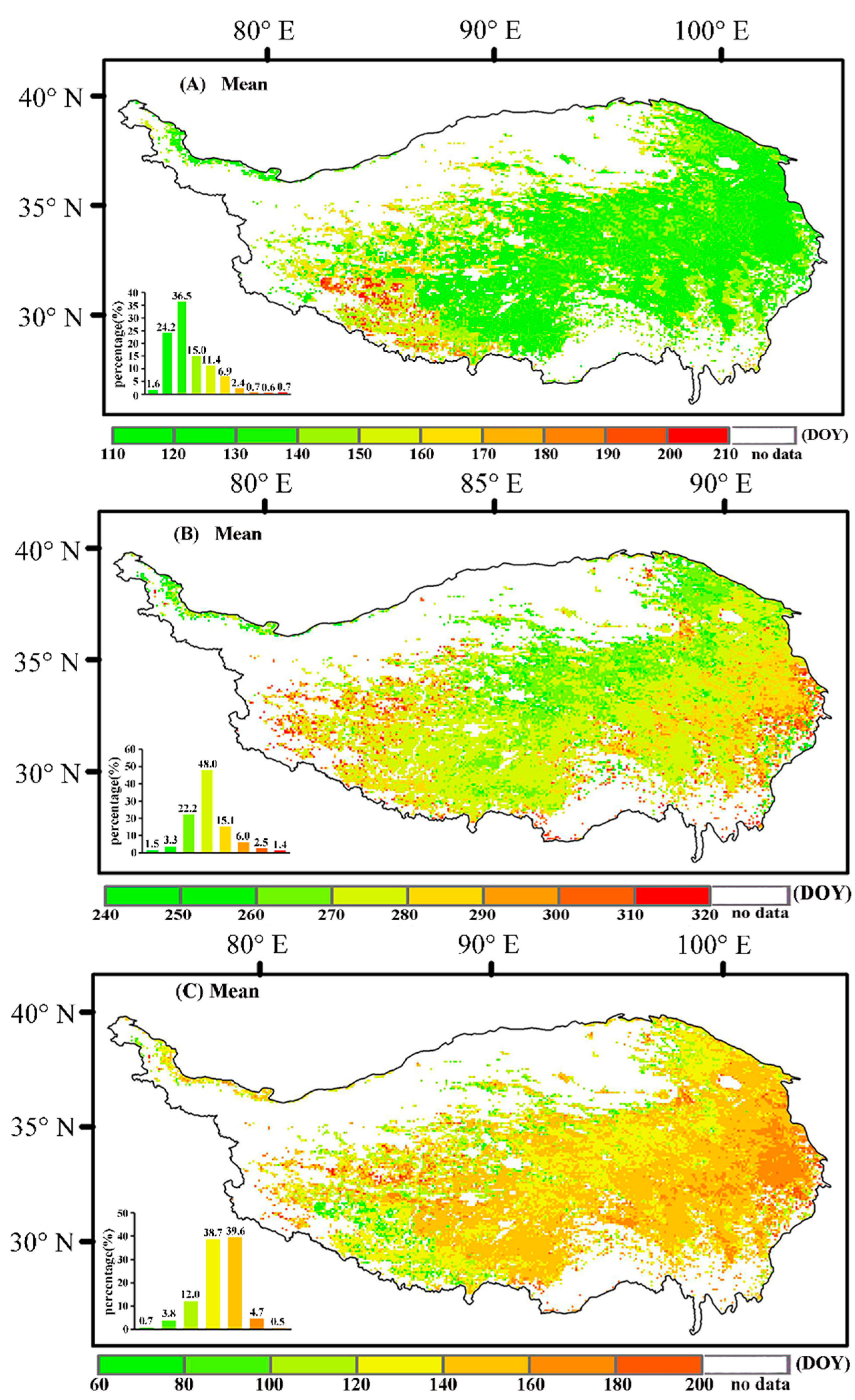
Analysis of vegetation phenology changes from 1982 to 2015 indicates that the SOS mainly occurred in mid-early May (Figure 3A), accounting for 60.70% of the total. Spatially, the SOS from the east to the west showed a gradual delay. The EOS at some point in October (Figure 3B), in both the east and the west, was delayed more than in the central regions. The LOS during the period 1982–2015 varied between 120 and 160 days (Figure 3C), accounting for approximately 78.30% of the total, whereas the LOS decreased gradually from the east to the west.
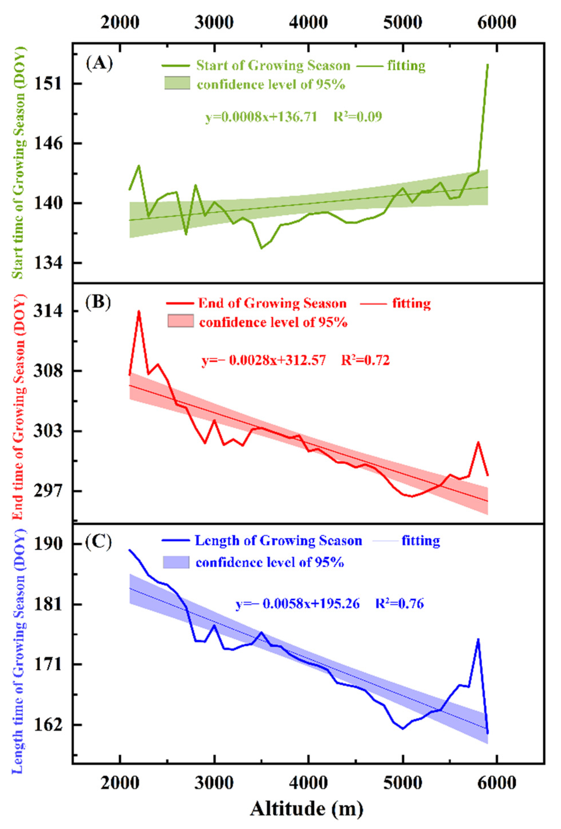
In analyzing the changes in vegetation phenology at various heights in the QTP from 1982 to 2015 (Figure 4), we realized that vegetation phenology varies with change in altitude. As per the findings, the following can be discerned (Figure 4): the SOS tends to be delayed approximately 0.08 days/100 m at an elevation between 2000 and 6000 m, while the EOS tends to by approximately 0.28 days/100 m. Overall, the LOS displayed sizeable decreases of approximately 0.58 days/100 m with an increase in altitude.
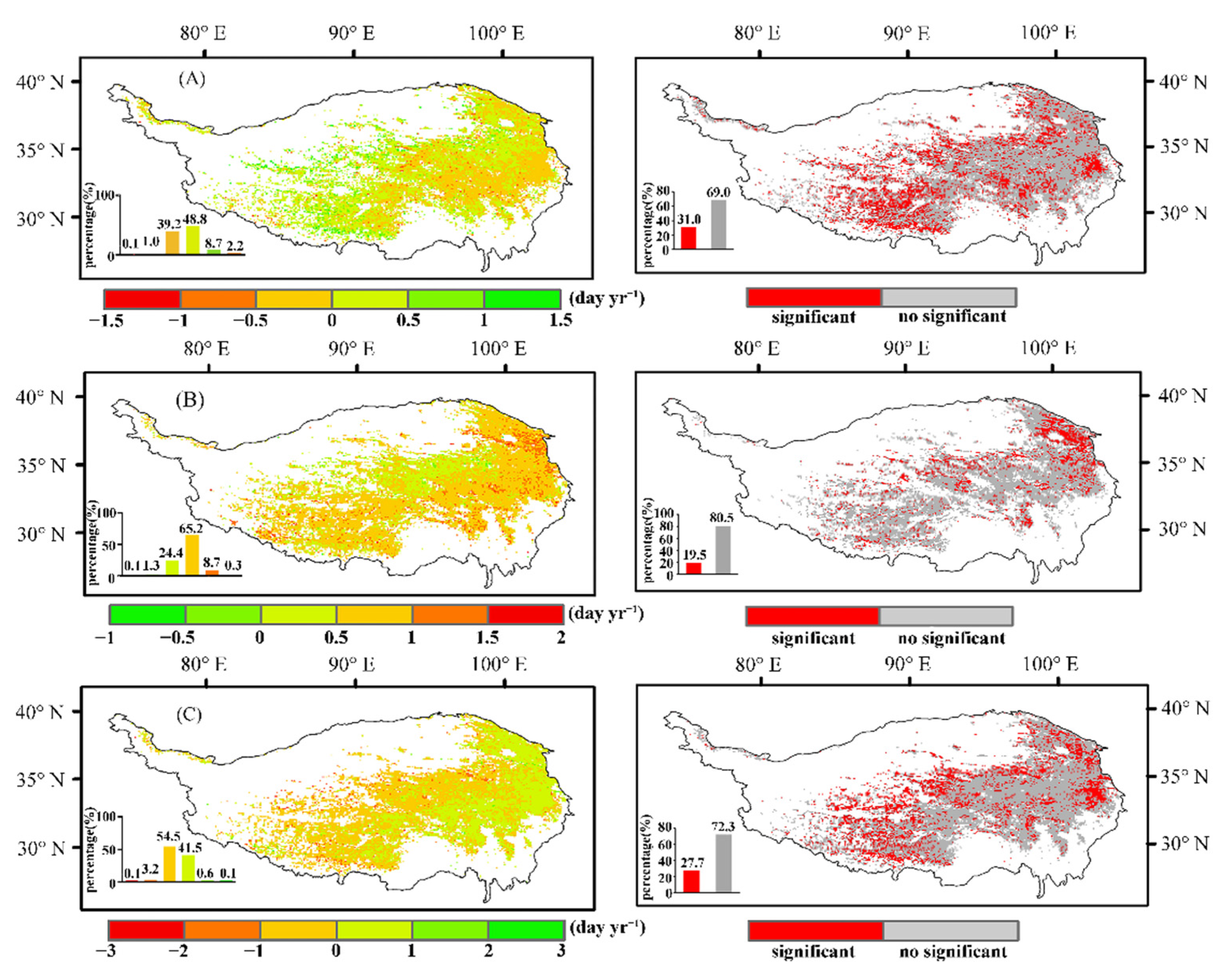
The past 30 years indicate change in the SOS is small (Figure 5A). Additionally, in the eastern and the central region of the study area, the trend shows an advance of approximately 0.19 days/a, while in the western region, the trend mainly shows a delay of approximately 0.29 days/a. There is a lagging trend of approximately 0.66 days/a for the EOS in 98.60% of the plateau (Figure 5B), with the west and the east lagging more than the central regions. On the other hand, the trend in the LOS in the eastern region is opposite to that in the central and the western regions (Figure 5C). Specifically, the LOS in the eastern plateau increased by approximately 0.31 days/a, while the LOS in the central and the western regions mostly decreased by approximately 0.42 days/a.
3.2. Relationship between Changes in Vegetation Phenology and Climatic Factors
In this section, first, we analyze the characteristics of different climatic factors, and then analyze the relationship between the growing season and climatic factors. Finally, we analyze the driving forces of the changes in vegetation phenology during the growing season.
3.2.1. Characteristics of Different Climatic Factors
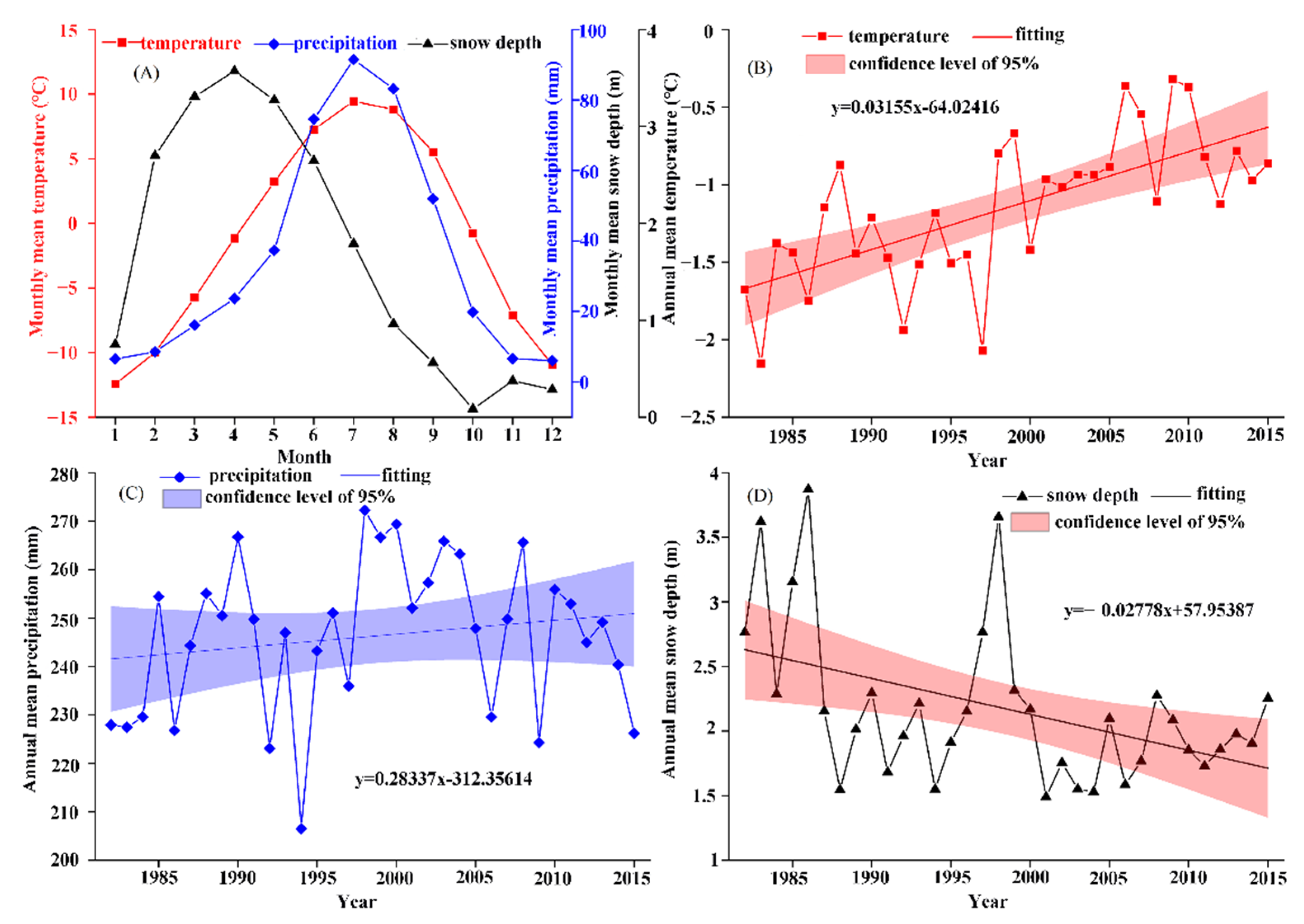
Analysis of annual changes in air temperature, precipitation, and snow depth in the QTP reveal that the maximum values of air temperature (9.46 °C) and precipitation (91.50 mm) occurred in July of each year, while the maximum value of snow depth (3.57 m) occurred in April (Figure 6A). From the perspective of interannual changes, the overall air temperature showed an upward trend (Figure 6B) of approximately 0.32 °C/decade from 1982 to 2015. Further, precipitation fluctuated greatly (Figure 6C), with the maximum value of annual precipitation topping out at approximately 1.32-fold the minimum value. Note that the maximum value occurred in 1998 and the minimum value in 1994.
Meanwhile, annual precipitation generally shows a gradual upward trend, but the increased range is not large (~2.8 mm/decade). Likewise, the change in snow depth is also relatively small for most years, with few exceptions. Specifically, snow depth remained at between 1.5 and 3 m (Figure 6D), with the maximum depth (3.87 m) occurring in 1986. For interannual change, the increment in air temperature resulted in the snow depth generally showing a gradual downward trend, decreasing by 0.28 m/decade.
3.2.2. Relationship between Growing Season and Climatic Factors
To analyze the relationship between the growing season and climatic factors, we first evaluate the relationship between the start of the growing season and climatic factors and then analyze the relationship between the end of the growing season and climatic factors.
Analysis of the Relationship between the Start of the Growing Season and Climatic Factors
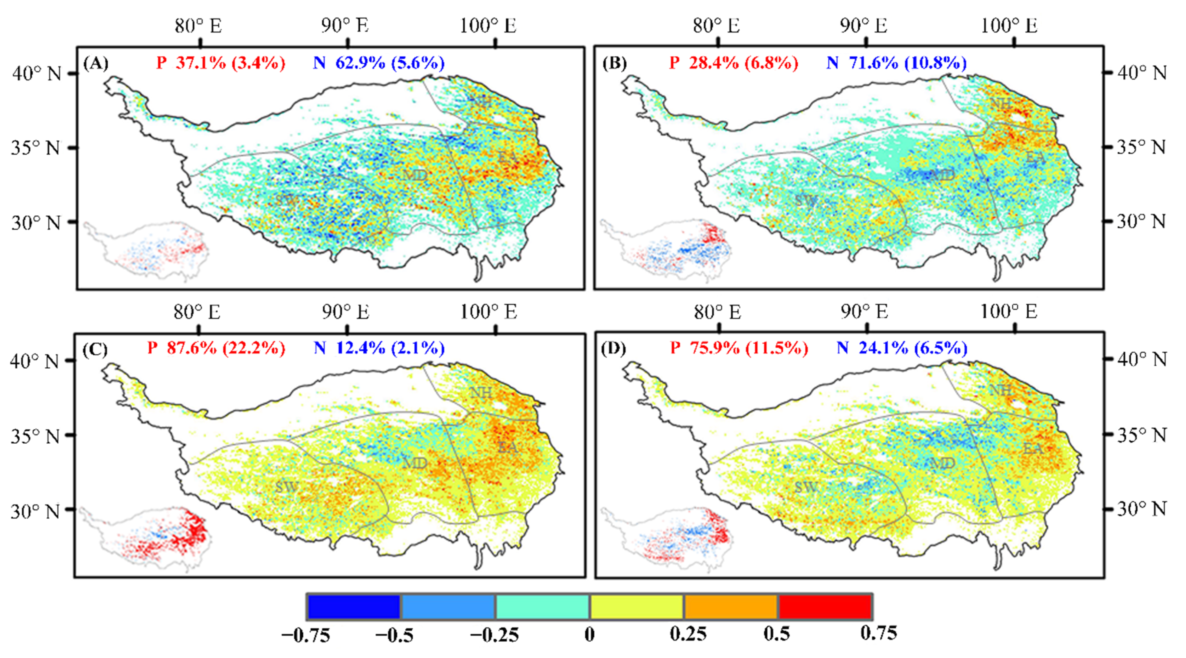
Across the QTP, the correlations between the interannual changes in the SOS and pre-season air temperature and precipitation are quite different in different regions (Figure 7). In the southwest, the SOS is positively correlated with pre-season air temperature and precipitation. In the east, the correlation is negative. However, there is significant correlation between the SOS and pre-season precipitation in the north of the QTP (p < 0.05).
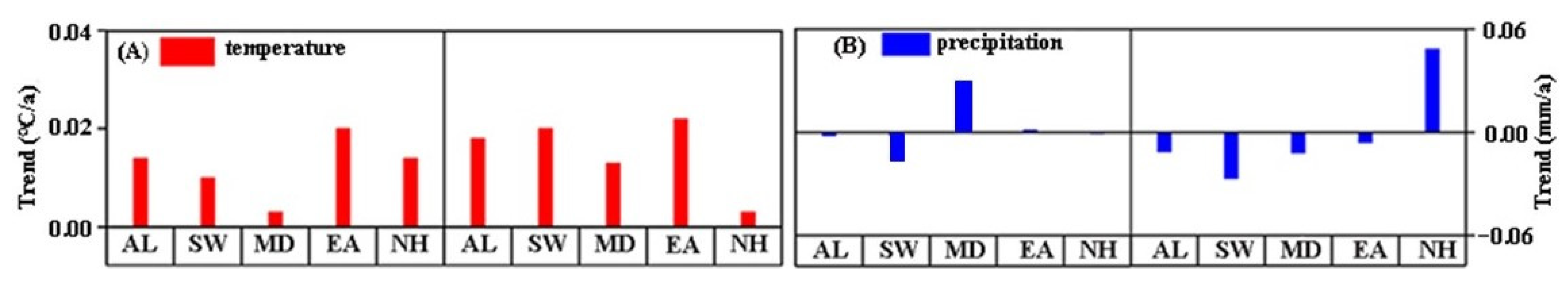
Throughout our analysis, we found that interannual changes in air temperature in different regions are consistent with the whole. Additionally, air temperature shows an upward trend over time. Specifically, the rise in air temperature in the east is greater than that of the QTP on the whole, which is approximately 0.20 °C/decade.
Further, we found that the interannual change in pre-season precipitation in the southwest and the north is consistent with the whole study region, displaying a decreasing trend, with the greatest decrease in the southwest by approximately 0.16 mm/decade. Nevertheless, the central and the eastern regions show the opposite trend. With time (year), precipitation shows an increasing trend, with the greatest increase in the central region at a rate of 0.30 mm/decade.
Analysis of the Relationship between the End of the Growing Season and Climatic Factors
On studying the correlation between pre-season air temperature, precipitation, and the end of the growing season from 1982 to 2015 (Figure 7), we realized that the areas with significant correlations are mainly distributed in the southwestern, northern, and eastern regions. To analyze how the changes in pre-season air temperature and precipitation across the above regions affected the end of the growing season, we studied the interannual changes in pre-season air temperature and precipitation. Our findings indicate that the interannual changes in air temperature and precipitation are displaying an opposite trend in the southwest. We found that pre-season air temperature causes the end of the growing season to lag (Figure 8).
In the north, there is a slow upward trend in the interannual changes in pre-season air temperature, which is higher than the overall trend. Furthermore, it can be seen that the slow increase in pre-season air temperature extends the growing season. On the other hand, the general trend in pre-season precipitation is opposite to the overall change in precipitation. When the overall precipitation shows a downward trend, the increase in precipitation in the north may be the main factor leading to the delay in the EOS.
In the east, we understand that the interannual changes in pre-season air temperature prior to the SOS show an upward trend that is higher than the overall change in air temperature, and that increasing air temperature results in a delay in the EOS. Moreover, when precipitation decreases, the end of the growing season advances, and the main reason for the delay in the EOS in the east may be the increase in pre-season air temperature.
3.2.3. Analysis of the Driving Forces of the Changes in Vegetation Phenology during the Growing Season
The different vegetation types in the QTP show enormous differences between the SOS, the EOS, and climatic factors in the pre-season, respectively (Table 1). Analysis of changes during the growing season of the different vegetation types indicates that grassland and shrubland are highly impacted by the factors in pre-season air temperature and precipitation (March, April, and May), accounting for 72.37% and 58.43%, respectively. The minimum value appears in the forest (29.36%). This suggests that grassland and shrubland in the region are greatly affected by climatic factors such as air temperature and precipitation, while forest areas are less affected.
Considering air temperature and precipitation in July, August, and September at the EOS, we see that pre-season air temperature and precipitation also have a great impact on grassland and shrubland, accounting for 58.96% and 62.95%, respectively. However, the end of the growing season in cropland area is less affected by these variables, accounting for only 36.57%.
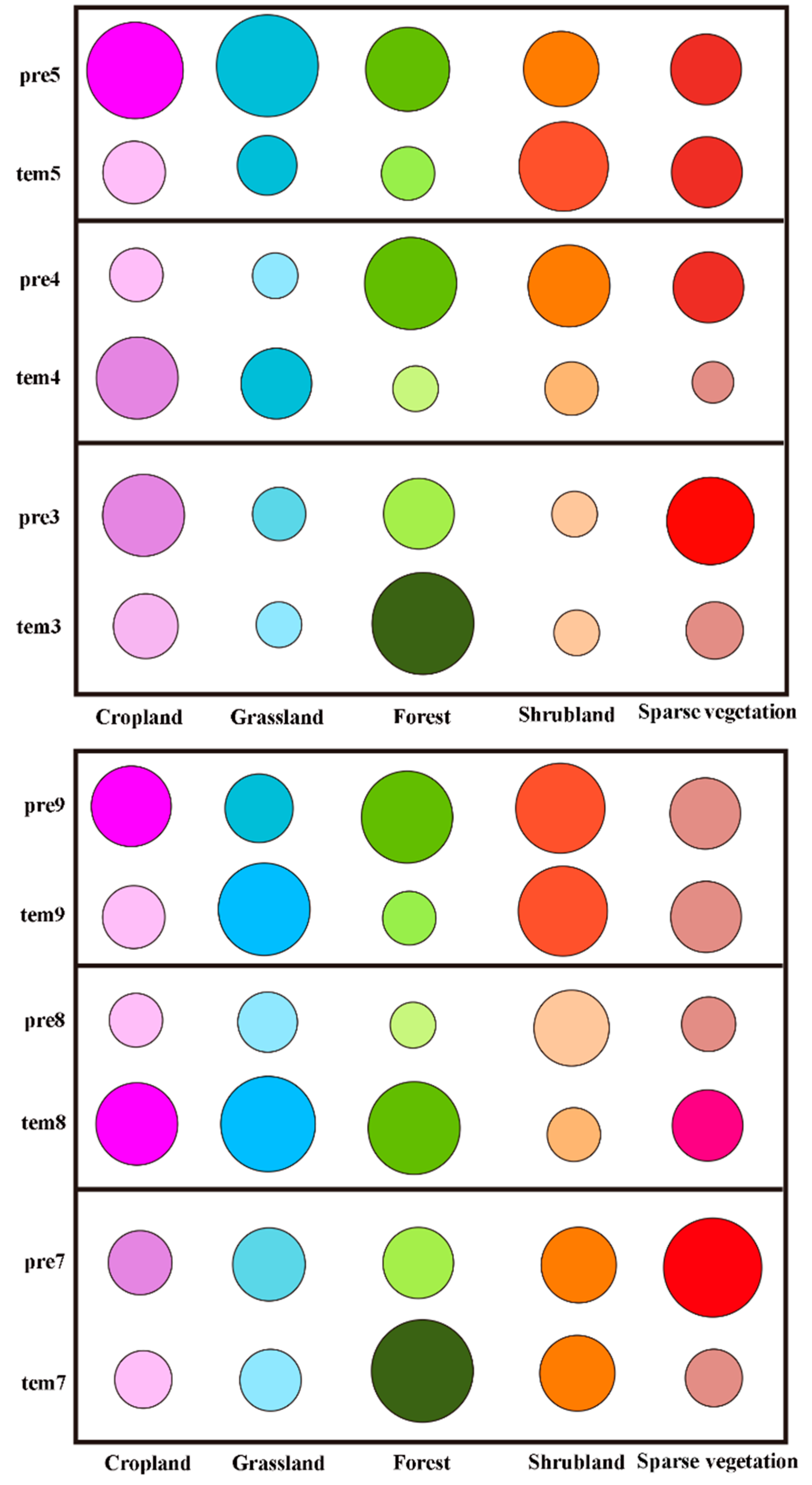
Similarly, the importance scores of the climatic factors affecting the SOS and the EOS in different vegetation regions and during different months show immense differences. First, by analyzing the importance scores of pre-season air temperature and precipitation with the SOS of the different vegetation types (Figure 9), we see that the vegetation phenology of cropland and grassland areas is mainly affected by air temperature in April and precipitation in May. However, the SOS of forest, shrubland, and sparse alpine vegetation is mainly impacted by air temperature or precipitation in March and April, respectively.
In addition, by analyzing the importance scores of pre-season air temperature and precipitation with the EOS of the different vegetation types, cropland and grassland are mainly affected by air temperature in August, while the EOS in shrubland is mainly affected by the air temperature and precipitation in September (Figure 9).
4. Discussion
In this section, we mainly discuss the following three aspects. First, we discuss the changes in vegetation phenology, then the response relationship between vegetation phenology and climatic factors, and finally the driving forces of the changes in vegetation phenology in the study area.
4.1. Changes in Vegetation Phenology in the Study Area
Interannual changes in vegetation phenology in the QTP from 1982 to 2015 showed varying degrees of fluctuation. The most pronounced changes occurred in 1998, with the SOS advancing the most and the LOS increasing the most. However, there was little change in the EOS at this time. This may be due to the higher air temperature and the maximum precipitation in the EOS that year [49], as the relationship between these two factors is beneficial for the germination of vegetation—it also greatly promotes the advance of the SOS, thus increasing the LOS.
From a spatial point of view, the SOS is gradually delayed from the east to the west in the study area, which is consistent with the results reported by Shen et al. [24]. In general, the EOS is earlier in the central region, but later in the eastern and western regions, which is similar to the results obtained by Li et al. for changes in the plateau’s vegetation phenology in the autumn of 1982–2012 [28]. Furthermore, it is consistent with the trend in the SOS in this area, indicating that changes in the SOS will also affect changes in the EOS [50]. Overall, there are notable differences in the spatial distribution of the LOS, which is mainly determined by the start and end times.
Air temperature is the main driving force of the SOS of alpine vegetation. Specifically, air temperature changes with altitude [24]. This study found that with an increase in altitude, the SOS fluctuated slightly in the plateau, showing a gentle upward trend. However, this correlation was weak, likely indicating that the change in the SOS has almost nothing to do with altitude [49].
Conversely, the correlation between the EOS, the LOS and the altitude is high (R2 > 0.7). With an increase in altitude, the EOS advances and the LOS decreases. This may be due to the relatively high air temperature at lower altitudes, which is beneficial for delaying leaf senescence and increasing carbon absorption of vegetation [51]. In other words, altitude promotes a delay in the EOS and lengthens the overall season. However, at higher altitudes, where air temperature is lower, the EOS advances to avoid harm from frost [51]. Thus, in these areas, there is a shorter growing season.
4.2. Response of Vegetation Phenology and Climatic Factors
Climatic factors profoundly impact vegetation phenology, with air temperature, in particular, playing an important role. Air temperature not only strongly affects the SOS [19,20], but also the EOS [21,22]. Along with air temperature, precipitation indicators are thought to have an important impact on vegetation phenology [52,53].
Most scholars studying the QTP generally believe that the increase in spring air temperatures is causing an advance in the SOS in alpine vegetation [23,54]. However, by observing the correlations between pre-season air temperature and precipitation in the southwest and the SOS, pre-season air temperature and precipitation are negatively correlated with the SOS; that is, the increase in pre-season air temperature and precipitation may lead to the advance of the SOS. Specifically, analyzing the interannual pre-season air temperature and precipitation in this region, it is found that air temperature shows an upward trend with time, while precipitation spirals downward, which is consistent with the results reported by Shen et al. obtained using 79 meteorological stations in the plateau from 2000 to 2011 [24]. These data also indicate that the advancing southwest growing season is mainly related to pre-season precipitation [24], because although air temperature charts an increasing trend, precipitation decreases. It is also worth noting that Kobresia littledalei C. B. Clarke and Potentilla fruticosa L. are the main dominant species in this region [55], and that these plants thrive in an environment of moderate air temperatures and high precipitation. Therefore, the decrease in precipitation greatly limits the growth of this particular vegetation and is not conducive to its germination, which leads to the delay in the SOS in this region.
The EOS in the southwest shows a positive correlation with pre-season air temperature and precipitation, while in the interannual change, air temperature increased but precipitation showed a downward trend, indicating that the increase in air temperature is the main factor leading to the lag in the EOS in the southwest. This is mainly because a small increase in air temperature has a positive effect on the delay in the EOS in this region, and an increase in precipitation would be unfavorable to the growth of this plant. Excessive water causes excessive soil moisture and leads to poor internal ventilation, resulting in the suffocation and ultimate death of the root system since it cannot absorb oxygen.
In the north of the Qinghai–Tibet Plateau, there is a positive correlation between the EOS and pre-season air temperature and precipitation, indicating that the increase in pre-season air temperature and precipitation can promote the lag in the EOS. These changes are likely the result of Stipa sareptana A.K. Becker var. krylovii (Roshev.) being the dominant species in this area [56]. The plant belongs to the family Gramineae and is a perennial dense herbaceous plant that mainly lives in a warm and drought-tolerant environment [56]. To a certain extent, the increase in air temperature is beneficial to the growth of the vegetation, and the increase in precipitation may also slow down the vegetation’s chlorophyll degradation rate [57]. The combined effect of the two may be the main reason for the delay in the EOS.
In the east, an increase in pre-season air temperature will delay the EOS, while pre-season precipitation tends to be stable, and it will also delay the EOS. This is mainly because the eastern plateau region has a warm and humid climate, and the vegetation type is mainly the alpine meadow [58]. The increase in air temperature will promote the growth of the vegetation, resulting in the delay in the EOS.
4.3. Analysis of the Driving Forces of the Changes in Vegetation Phenology
The phenology of the different vegetation types is affected by climatic factors to varying degrees [59]. On analyzing the response relationship between the SOS, the EOS and pre-season climatic factors, we found that areas with a higher response relationship between the SOS and pre-season air temperature and precipitation are mainly in the grassland and shrubland. These factors have the lowest impact on the forest, which may be related to the importance scores of various climatic factors across different regions. Thus, for cropland and grassland, air temperature in April and precipitation in May significantly impact the SOS. However, forest and shrubland are mainly affected by pre-season precipitation in April, which shows that pre-season precipitation is the main factor that affects the difference between them, because the taller shrub and forest plants mainly grow in warmer areas and display high water consumption, so an early increase in pre-season precipitation will lead to the increase in vegetation photosynthesis, and increase the nutrient content of the vegetation [60]. However, this is not possible for grassland and cropland with a late growing season [61].
In addition, precipitation in April or May is the main driving force of the SOS in different vegetation. This is primarily due to the different demand for precipitation in the various areas of vegetation. Specifically, vegetation in the southwest thrives in wet conditions, while vegetation in the north is drought- tolerant. So, both more and less precipitation will cause changes in the SOS.
Air temperature in August is the key factor influencing the EOS in cropland, grassland and forest. This is caused by these plant types being mainly distributed in the north and west of the study area, where air temperature is typically high, leading to the growth of drought- tolerant vegetation. Moreover, because the key period of vegetation growth and also the time of year with the highest air temperatures is August, further increases in air temperature this point will enhance the photosynthetic rate of vegetation, thus reducing the degradation rate of chlorophyll with vegetation aging [29] as well as reducing sufficient nutrients for growth, and consequently affecting the EOS.
For other vegetation, air temperature and precipitation in September are important driving forces of the EOS, which may be due to the EOS being mainly concentrated from the end of September to the beginning of October. The climatic factors affecting the first month of the pre-season are most closely related to vegetation phenology in the growing season.
5. Conclusions
This research investigated the characteristics of the spatial changes in vegetation phenology in the QTP over a recent 34 years period. This study also analyzed the mutual feedback mechanisms between vegetation phenology and climate and explored the main climate-related driving forces of the phenology of the different vegetation types. Based on the GIMMS3g data of time series from 1982 to 2015, we observed that the interannual changes in vegetation phenology in the study area fluctuated to different degrees. Spatially, the SOS shows an advancing trend from the east to the west. With an increase in altitude, this trend was less evident, but there were pronounced changes in both the EOS and the LOS.
Additionally, we examined how pre-season air temperature and precipitation impact vegetation phenology, finding that the SOS in the southwest and the north may be related to the decrease in pre-season precipitation, which leads to the delay in the growing season in the southwest and the advance in the growing season in the north. Except for the central region of the study area, an increase in air temperature in other areas will delay the EOS, and a decrease in pre-season precipitation will advance the EOS in the southwest and the east. The increase in pre-season precipitation leads to the delay in the growing season in the north. The main reason for the above phenomenon is that the dominant species of vegetation in different regions have different responses to hydrothermal conditions.
In addition, we found that in the growing season, cropland and grassland are greatly affected by climatic factors. Pre-season precipitation in April or May is the main factor affecting the SOS of the different vegetation types, while pre-season air temperature and precipitation together affect the change in EOS.
6. Shortcomings and Future Works
In this paper, the driving forces of the changes in vegetation phenology on the Qinghai–Tibet Plateau were analyzed, but there are still some areas that need to be further explored in-depth. We only analyzed the effects of temperature and precipitation, the main driving forces of vegetation phenology in this region [62].We left human factors unexplored, but these also affect vegetation changes; for example, overgrazing, the increase in population, the increase in agricultural production area and fire can affect the vegetation [63,64,65]. In addition, land cover types that are not natural vegetation and errors in the climate datasets maybe also affecting the changes in vegetation phenology.
Given the above shortcomings, we will perform related work considering the following three factors in the future. Since the spatial resolution of the GIMMS3g NDVI dataset is low, and the period is only from 1982 to 2015, future studies should integrate a series of products over a longer time and at a higher resolution to further discuss the response relationship between vegetation phenology and climate change. Second, the results in this paper are based on remote sensing data, and they need to be further verified in the future by combining field monitoring and process-based ecosystem models. Third, study of the impact of climatic factors and human activities on vegetation phenology in this area is open to future scholars. Nevertheless, the results of this paper have implications for predicting the future evolution of ecosystems and implementing effective ecosystem management.
Author Contributions
Conceptualization, X.L. and Y.C.; methodology, Y.C.; software, M.Z.; validation, X.L., Y.L. and Z.L.; writing—original draft preparation, X.L.; writing—review and editing, X.L., Y.L., Q.Z. and Y.C.; funding acquisition, Z.L. All authors have read and agreed to the published version of the manuscript.
Funding
This research was funded by the National Natural Science Foundation of China (41971141) and National Key Research and Development Program (2019YFA0606902), also the Youth Innovation Promotion Association of the Chinese Academy of Sciences (No. 2018480).
Institutional Review Board Statement
Not applicable.
Informed Consent Statement
Not applicable.
Data Availability Statement
The data presented in this study are available on request from the corresponding author.
Conflicts of Interest
The authors declare no conflict of interest.
References
- Parmesan, C. Ecological and evolutionary responses to recent climate change. Annu. Rev. Ecol. Evol. Syst. 2006, 37, 637–669. [Google Scholar] [CrossRef] [Green Version]
- Linderholm, H.W. Growing season changes in the last century. Agric. For. Meteorol. 2006, 137, 1–14. [Google Scholar] [CrossRef]
- Richardson, A.D.; Keenan, T.F.; Migliavacca, M.; Ryu, Y.; Sonnentag, O.; Toomey, M. Climate change, phenology, and phenological control of vegetation feedbacks to the climate system. Agric. For. Meteorol. 2013, 169, 156–173. [Google Scholar] [CrossRef]
- Walther, G.R.; Post, E.; Convey, P.; Menzel, A.; Parmesan, C.; Beebee, T.J.C.; Fromentin, J.-M.; Hoegh-Guldberg, O.; Bairlein, F. Ecological responses to recent climate change. Nature 2002, 416, 389–395. [Google Scholar] [CrossRef] [PubMed]
- Kelly, A.E.; Goulden, M.L. Rapid shifts in plant distribution with recent climate change. Proc. Natl. Acad. Sci. USA 2008, 105, 11823–11826. [Google Scholar] [CrossRef] [Green Version]
- Wu, D.; Zhao, X.; Liang, S.; Zhou, T.; Huang, K.; Tang, B.; Zhao, W. Time-lag effects of global vegetation responses to climate change. Glob. Chang. Biol. 2015, 21, 3520–3531. [Google Scholar] [CrossRef] [PubMed]
- Zhou, L.; Tian, Y.; Myneni, R.B.; Ciais, P.; Saatchi, S.; Liu, Y.Y.; Piao, S.; Chen, H.; Vermote, E.F.; Song, C. Widespread decline of Congo rainforest greenness in the past decade. Nature 2014, 509, 86–90. [Google Scholar] [CrossRef]
- Peñuelas, J.; Filella, I. Phenology feedbacks on climate change. Science 2009, 324, 887–888. [Google Scholar] [CrossRef] [PubMed] [Green Version]
- Tan, J.; Piao, S.; Chen, A.; Zeng, Z.; Ciais, P.; Janssens, I.A.; Mao, J.; Myneni, R.B.; Peng, S.; Peñuelas, J. Seasonally different response of photosynthetic activity to daytime and night-time warming in the Northern Hemisphere. Glob. Change Biol. 2015, 21, 377–387. [Google Scholar] [CrossRef] [PubMed]
- Lieth, H. Phenology and Seasonality Modeling; Springer: Berlin/Heidelberg, Germany, 1974. [Google Scholar]
- Piao, S.; Liu, Q.; Chen, A.; Janssens, I.A.; Fu, Y.; Dai, J.; Liu, L.; Lian, X.; Shen, M.; Zhu, X. Plant phenology and global climate change: Current progresses and challenges. Glob. Chang. Biol. 2019, 25, 1922–1940. [Google Scholar] [CrossRef]
- Xie, Y.; Wang, X.; Silander, J.A. Deciduous forest responses to temperature, precipitation, and drought imply complex climate change impacts. Proc. Natl. Acad. Sci. USA 2015, 112, 13585–13590. [Google Scholar] [CrossRef] [PubMed] [Green Version]
- Tang, J.; Körner, C.; Muraoka, H.; Piao, S.; Shen, M.; Thackeray, S.J.; Yang, X.J.E. Emerging opportunities and challenges in phenology: A review. Ecosphere 2016, 7, e01436. [Google Scholar] [CrossRef] [Green Version]
- Visser, M.E. Interactions of climate change and species. Nature 2016, 535, 236–237. [Google Scholar] [CrossRef] [PubMed]
- Piao, S.; Friedlingstein, P.; Ciais, P.; Viovy, N.; Demarty, J. Growing season extension and its impact on terrestrial carbon cycle in the Northern Hemisphere over the past 2 decades. Glob. Biogeochem. Cycle 2007, 21, GB3018. [Google Scholar] [CrossRef]
- Richardson, A.D.; Hollinger, D.Y.; Dail, D.B.; Lee, J.T.; Munger, J.W. Influence of spring phenology on seasonal and annual carbon balance in two contrasting New England forests. Tree Physiol. 2009, 29, 321–331. [Google Scholar] [CrossRef]
- Churkina, G.; Schimel, D.; Braswell, B.H.; Xiao, X. Spatial analysis of growing season length control over net ecosystem exchange. Glob. Chang. Biol. 2005, 11, 1777–1787. [Google Scholar] [CrossRef]
- Jeong, S.J.; Medvigy, D.; Shevliakova, E.; Malyshev, S. Uncertainties in terrestrial carbon budgets related to spring phenology. J. Geophys. Res. Biogeosci. 2012, 117, G01030. [Google Scholar] [CrossRef]
- Bigler, C.; Vitasse, Y. Daily maximum temperatures induce lagged effects on leaf unfolding in temperate woody species across large elevational gradients. Front. Plant. Sci. 2019, 10, 398. [Google Scholar] [CrossRef] [Green Version]
- Fu, Y.H.; Zhao, H.; Piao, S.; Peaucelle, M.; Peng, S.; Zhou, G.; Ciais, P.; Huang, M.; Menzel, A.; Peñuelas, J. Declining global warming effects on the phenology of spring leaf unfolding. Nature 2015, 526, 104–107. [Google Scholar] [CrossRef] [PubMed] [Green Version]
- Fu, Y.H.; Piao, S.; Delpierre, N.; Hao, F.; Hänninen, H.; Liu, Y.; Sun, W.; Janssens, I.A.; Campioli, M. Larger temperature response of autumn leaf senescence than spring leaf-out phenology. Glob. Chang. Biol. 2018, 24, 2159–2168. [Google Scholar] [CrossRef] [PubMed]
- Garonna, I.; De Jong, R.; De Wit, A.J.; Mücher, C.A.; Schmid, B.; Schaepman, M.E. Strong contribution of autumn phenology to changes in satellite-derived growing season length estimates across Europe (1982–2011). Glob. Chang. Biol. 2014, 20, 3457–3470. [Google Scholar] [CrossRef]
- Zhang, G.; Zhang, Y.; Dong, J.; Xiao, X. Green-up dates in the Tibetan Plateau have continuously advanced from 1982 to 2011. Proc. Natl. Acad. Sci. USA 2013, 110, 4309–4314. [Google Scholar] [CrossRef] [PubMed] [Green Version]
- Shen, M.; Zhang, G.; Cong, N.; Wang, S.; Kong, W.; Piao, S. Increasing altitudinal gradient of spring vegetation phenology during the last decade on the Qinghai–Tibetan Plateau. Agric. For. Meteorol. 2014, 189, 71–80. [Google Scholar] [CrossRef]
- Zhang, Q.; Kong, D.; Shi, P.; Singh, V.P.; Sun, P. Vegetation phenology on the Qinghai-Tibetan Plateau and its response to climate change (1982–2013). Agric. For. Meteorol. 2018, 248, 408–417. [Google Scholar] [CrossRef]
- Che, M.; Chen, B.; Innes, J.L.; Wang, G.; Dou, X.; Zhou, T.; Zhang, H.; Yan, J.; Xu, G.; Zhao, H. Spatial and temporal variations in the end date of the vegetation growing season throughout the Qinghai–Tibetan Plateau from 1982 to 2011. Agric. For. Meteorol. 2014, 189, 81–90. [Google Scholar] [CrossRef]
- Ding, M.; Zhang, Y.; Sun, X.; Liu, L.; Wang, Z.; Bai, W. Spatiotemporal variation in alpine grassland phenology in the Qinghai-Tibetan Plateau from 1999 to 2009. Chin. Sci. Bull. 2013, 58, 396–405. [Google Scholar] [CrossRef] [Green Version]
- Li, P.; Zhu, Q.; Peng, C.; Zhang, J.; Wang, M.; Zhang, J.; Ding, J.; Zhou, X. Change in Autumn Vegetation Phenology and the Climate Controls From 1982 to 2012 on the Qinghai-Tibet Plateau. Front. Plant. Sci. 2020, 10, 1677. [Google Scholar] [CrossRef] [Green Version]
- Liu, Q.; Fu, Y.H.; Zeng, Z.Z.; Huang, M.T.; Li, X.R.; Piao, S.L. Temperature, precipitation, and insolation effects on autumn vegetation phenology in temperate China. Glob. Chang. Biol. 2016, 22, 644–655. [Google Scholar] [CrossRef] [PubMed]
- Piao, S.; Fang, J.; Zhou, L.; Ciais, P.; Zhu, B. Variations in satellite-derived phenology in China’s temperate vegetation. Glob. Chang. Biol. 2006, 12, 672–685. [Google Scholar] [CrossRef]
- Pinzon, J.E.; Tucker, C.J. A Non-Stationary 1981–2012 AVHRR NDVI3g Time Series. Remote Sens. 2014, 6, 6929–6960. [Google Scholar] [CrossRef] [Green Version]
- Zhang, G.; Yao, T.; Xie, H.; Yang, K.; Zhu, L.; Shum, C.; Bolch, T.; Yi, S.; Allen, S.; Jiang, L. Response of Tibetan Plateau’s lakes to climate changes: Trend, pattern, and mechanisms. Earth-Sci. Rev. 2020, 208, 103269. [Google Scholar] [CrossRef]
- Immerzeel, W.W.; van Beek, L.P.H.; Bierkens, M.F.P. Climate Change Will Affect the Asian Water Towers. Science 2010, 328, 1382–1385. [Google Scholar] [CrossRef]
- Immerzeel, W.W.; Lutz, A.; Andrade, M.; Bahl, A.; Biemans, H.; Bolch, T.; Hyde, S.; Brumby, S.; Davies, B.; Elmore, A. Importance and vulnerability of the world’s water towers. Nature 2020, 577, 364–369. [Google Scholar] [CrossRef] [PubMed]
- Cheng, S.K.; Shen, R. Discussion on the interaction among population, Resources, Environment and Development in Qinghai-Tibet Plateau. J. Nat. Resour. 2000, 15, 297–304. [Google Scholar]
- Kang, S.; Xu, Y.; You, Q.; Flügel, W.-A.; Pepin, N.; Yao, T. Review of climate and cryospheric change in the Tibetan Plateau. Environ. Res. Lett. 2010, 5, 015101. [Google Scholar] [CrossRef]
- Hollmann, R.; Merchant, C.J.; Saunders, R.; Downy, C.; Buchwitz, M.; Cazenave, A.; Chuvieco, E.; Defourny, P.; de Leeuw, G.; Forsberg, R. The ESA climate change initiative: Satellite data records for essential climate variables. Bull. Am. Meteorol. Soc. 2013, 94, 1541–1552. [Google Scholar] [CrossRef] [Green Version]
- Shen, M.; Sun, Z.; Wang, S.; Zhang, G.; Kong, W.; Chen, A. No evidence of continuously advanced green-up dates in the Tibetan Plateau over the last decade. Proc. Natl. Acad. Sci. USA 2013, 110, E2329. [Google Scholar] [CrossRef] [Green Version]
- Tan, B.; Morisette, J.; Wolfe, R.; Gao, F.; Ederer, G.; Nightingale, J. An enhanced TIMESAT algorithm for estimating vegetation phenology metrics from MODIS data. IEEE J.-STARS. 2011, 4, 361–371. [Google Scholar] [CrossRef]
- Chen, J.; Jönsson, P.; Tamura, M.; Gu, Z.; Matsushita, B.; Eklundh, L. A simple method for reconstructing a high-quality NDVI time-series data set based on the Savitzky–Golay filter. Remote Sens. Environ. 2004, 91, 332–344. [Google Scholar] [CrossRef]
- White, M.A.; Beurs, K.M.D.; Didan, K.; Inouye, D.W.; Richardson, A.D.; Jensen, O.P. Intercomparison, interpretation, and assessment of spring phenology in North America estimated from remote sensing for 1982–2006. Glob. Chang. Biol. 2009, 15, 2335–2359. [Google Scholar] [CrossRef]
- Hufkens, K.; Friedl, M.; Sonnentag, O.; Braswell, B.H.; Milliman, T.; Richardson, A.D. Linking near-surface and satellite remote sensing measurements of deciduous broadleaf forest phenology. Remote Sens. Environ. 2012, 117, 307–321. [Google Scholar] [CrossRef]
- Jonsson, P.; Eklundh, L. Seasonality extraction by function fitting to time-series of satellite sensor data. IEEE Trans. Geosci. Remote Sens. 2002, 40, 1824–1832. [Google Scholar] [CrossRef]
- Yu, H.; Luedeling, E.; Xu, J. Winter and spring warming result in delayed spring phenology on the Tibetan Plateau. Proc. Natl. Acad. Sci. USA 2010, 107, 22151–22156. [Google Scholar] [CrossRef] [PubMed] [Green Version]
- Mann, H.B. Nonparametric tests against trend. Econometrica 1945, 13, 245–259. [Google Scholar] [CrossRef]
- Breiman, L. Random forests. Mach. Learn. 2001, 45, 5–32. [Google Scholar] [CrossRef] [Green Version]
- Kelsey, K.C.; Pedersen, S.H.; Leffler, A.J.; Sexton, J.O.; Feng, M.; Welker, J.M. Winter snow and spring temperature have differential effects on vegetation phenology and productivity across Arctic plant communities. Glob. Chang. Biol. 2021, 27, 1572–1586. [Google Scholar] [CrossRef]
- Liaw, A.; Wiener, M. Classification and regression by randomForest. R News 2002, 2, 18–22. [Google Scholar] [CrossRef]
- Piao, S.; Cui, M.; Chen, A.; Wang, X.; Ciais, P.; Liu, J.; Tang, Y. Altitude and temperature dependence of change in the spring vegetation green-up date from 1982 to 2006 in the Qinghai-Xizang Plateau. Agric. For. Meteorol. 2011, 151, 1599–1608. [Google Scholar] [CrossRef]
- Keenan, T.F.; Richardson, A.D. The timing of autumn senescence is affected by the timing of spring phenology: Implications for predictive models. Glob. Chang. Biol. 2015, 21, 2634–2641. [Google Scholar] [CrossRef] [Green Version]
- Chen, L.; Hänninen, H.; Rossi, S.; Smith, N.G.; Pau, S.; Liu, Z.; Feng, G.; Gao, J.; Liu, J. Leaf senescence exhibits stronger climatic responses during warm than during cold autumns. Nat. Clim. Chang. 2020, 10, 777–780. [Google Scholar] [CrossRef]
- Wipf, S. Phenology, growth, and fecundity of eight subarctic tundra species in response to snowmelt manipulations. Plant. Ecol. 2010, 207, 53–66. [Google Scholar] [CrossRef] [Green Version]
- Krab, E.J.; Roennefarth, J.; Becher, M.; Blume-Werry, G.; Keuper, F.; Klaminder, J.; Kreyling, J.; Makoto, K.; Milbau, A.; Dorrepaal, E. Winter warming effects on tundra shrub performance are species-specific and dependent on spring conditions. J. Ecol. 2018, 106, 599–612. [Google Scholar] [CrossRef]
- Shen, M. Spring phenology was not consistently related to winter warming on the Tibetan Plateau. Proc. Natl. Acad. Sci. USA 2011, 108, E91–E92. [Google Scholar] [CrossRef] [Green Version]
- Wei, W.; Zhou, J.; Bai, M.; Qu, G. Investigation on Kobresia resources in Tibet Plateau. Wild Plant. Res. China 2019, 38, 80–85. [Google Scholar] [CrossRef]
- Xu, W.; Xin, Y.; Zhang, J.; Xiao, R.; Wang, X. Changes in growth period of grasses in northeastern Qinghai-Tibet Plateau in recent 20 years. Acta Ecol. Sin. 2014, 34, 1781–1793. [Google Scholar] [CrossRef] [Green Version]
- Vicente-Serrano, S.M.; Gouveia, C.; Camarero, J.J.; Beguería, S.; Trigo, R.; López-Moreno, J.I.; Azorín-Molina, C.; Pasho, E.; Lorenzo-Lacruz, J.; Revuelto, J.; et al. Response of vegetation to drought time-scales across global land biomes. Proc. Natl. Acad. Sci. USA 2013, 110, 52–57. [Google Scholar] [CrossRef] [Green Version]
- Hou, M.; Gao, J.; Ge, J.; Li, Y.; Jassamyn, L.; Yin, J.; Feng, Q.; Liang, T. Study on dynamic changes and driving factors of alpine swamp wetlands in eastern Qinghai-Tibet Plateau. Acta Pratac. Sin. 2020, 29, 13–27. [Google Scholar] [CrossRef]
- Shen, X.; Xue, Z.; Jiang, M.; Lu, X. Spatiotemporal change of vegetation coverage and its relationship with climate change in freshwater marshes of Northeast China. Wetlands. 2019, 39, 429–439. [Google Scholar] [CrossRef]
- Starr, G.; Oberbauer, S.F. Photosynthesis of Arctic Evergreens under Snow: Implications for Tundra Ecosystem Carbon Balance. Ecology 2003, 84, 1415–1420. [Google Scholar] [CrossRef]
- Bell, K.L.; Bliss, L. Autecology of Kobresia bellardii: Why winter snow accumulation limits local distribution. Ecol. Monogr. 1979, 49, 377–402. [Google Scholar] [CrossRef]
- Huang, K.; Zhang, Y.; Zhu, J.; Liu, Y.; Zu, J.; Zhang, J. The influences of climate change and human activities on vegetation dynamics in the Qinghai-Tibet Plateau. Remote Sens. 2016, 8, 876. [Google Scholar] [CrossRef] [Green Version]
- Pereira, P.; Cerdà, A.; Lopez, A.J.; Zavala, L.M.; Mataix-Solera, J.; Arcenegui, V.; Misiune, I.; Keesstra, S.; Novara, A. Short-term vegetation recovery after a grassland fire in Lithuania: The effects of fire severity, slope position and aspect. Land Degrad Dev. 2016, 27, 1523–1534. [Google Scholar] [CrossRef]
- Wu, W.-B.; Ma, J.; Meadows, M.E.; Banzhaf, E.; Huang, T.-Y.; Liu, Y.-F.; Zhao, B. Spatio-temporal changes in urban green space in 107 Chinese cities (1990–2019): The role of economic drivers and policy. Int. J. Appl. Earth Obs. Geoinf. 2021, 103, 102525. [Google Scholar] [CrossRef]
- Li, P.; Peng, C.; Wang, M.; Luo, Y.; Li, M.; Zhang, K.; Zhang, D.; Zhu, Q. Dynamics of vegetation autumn phenology and its response to multiple environmental factors from 1982 to 2012 on Qinghai-Tibetan Plateau in China. Sci. Total Environ. 2018, 637–638, 855–864. [Google Scholar] [CrossRef] [PubMed]
Figure 1.
Location of the QTP and the distribution of the different vegetation types. The different color legends in the upper left represent all of the vegetation types in the study area. The lower left in the figure represents the location of the study area in the world.
Figure 1.
Location of the QTP and the distribution of the different vegetation types. The different color legends in the upper left represent all of the vegetation types in the study area. The lower left in the figure represents the location of the study area in the world.

Figure 2.
Characteristics of the interannual changes in vegetation phenology. The green, red and blue lines represent the interannual changes in SOS, the EOS, and the LOS, respectively. The blue and green equations at the upper left of the graph represent the interannual changes in 1982 to 1998, respectively. The blue and green equations at the lower right of the graph represent the interannual changes in 1998 to 2015, respectively. The red equation at the lower left represents the interannual changes in 1982 to 2015. Days of Year (DOY) represents the change in the vegetation growing season in the study area.

Figure 3.
Characteristics of the changes in vegetation phenology. (A–C) represent the average changes in the SOS, the EOS, and the LOS from 1982 to 2015, respectively. The histogram in the lower left represents the percentage of different color bands in the total number.
Figure 3.
Characteristics of the changes in vegetation phenology. (A–C) represent the average changes in the SOS, the EOS, and the LOS from 1982 to 2015, respectively. The histogram in the lower left represents the percentage of different color bands in the total number.

Figure 4.
Characteristics of the changes in vegetation phenology with altitude. (A–C) represent the average changes in the SOS, the EOS, and the LOS from 1982 to 2015 at different elevations, respectively.
Figure 4.
Characteristics of the changes in vegetation phenology with altitude. (A–C) represent the average changes in the SOS, the EOS, and the LOS from 1982 to 2015 at different elevations, respectively.

Figure 5.
Changes in vegetation phenology during different periods of the growing season. (A–C) represent the trend in the start, the end, and the length of the growing season from 1982 to 2015, respectively. The right side of each trend chart is significant according to the M-K test (p < 0.05). In the lower left of the bar chart, red represents the proportion of the number of regions with a significant trend (p < 0.05). Gray represents the proportion of the number of areas with a non-significant trend.

Figure 6.
Annual and monthly change in climatic factors. (A) represents the monthly average of air temperature, precipitation and snow depth from 1982 to 2015 in the study area, while (B–D) represent the monthly average of air temperature, precipitation, and snow depth from 1982 to 2015, respectively.

Figure 7.
The correlation between vegetation phenology and pre-season climatic factors. (A,B) represent the correlation between the SOS and pre-season air temperature and precipitation, respectively. (C,D) represent the correlation between the EOS and pre-season air temperature and precipitation, respectively. The inset panels in the lower left of each submap present pixels with a significantly (p < 0.05) positive (red) and negative (blue) value. The percentages of positive (P) and negative (N) correlations (percentage of significant correlations in parentheses) are shown at the top of each submap. SW, MD, EA and NH represent the southwestern, middle, eastern and northern regions of the study area, respectively.

Figure 8.
Trends in air temperature and precipitation in different areas of the study area. (A,B) represent the interannual changes in pre-season air temperature and precipitation in different areas of the study area, respectively. The left half of (A) presents the interannual changes in air temperature at the SOS, and the right half presents the interannual changes in air temperature at the EOS. The left half of (B) presents the interannual changes in precipitation at the SOS, and the right half presents the interannual changes in precipitation at the EOS. AL, SW, MD, EA, and NH represent all of and the southwestern, middle, eastern, and northern regions of the study area, respectively.

Figure 9.
The importance scores of the pre-season climatic factors affecting the SOS and the EOS of different vegetation types during different months. The horizontal axes represent the different vegetation types in the study area. tem3, tem4, and tem5 represent air temperature in March, April, and May from 1982 to 2015, respectively. pre3, pre4, and pre5 represent precipitation in March, April, and May from 1982 to 2015, respectively. tem7, tem8, and tem9 represent air temperature in July, August, and September from 1982 to 2015, respectively. pre7, pre8, and pre9 represent precipitation in July, August, and September from 1982 to 2015, respectively. The colored circle size represents the importance score of different indicators—the larger the circle, the higher the score.


Table 1.
Interpretation of different climatic factors affecting the different vegetation types.
| Vegetation Type | SOS (%) | EOS (%) |
|---|---|---|
| Cropland | 47.28 | 36.57 |
| Grassland | 72.37 | 58.96 |
| Forest | 29.36 | 45.88 |
| Shrubland | 58.43 | 62.95 |
| Sparse vegetation | 42.81 | 37.82 |
Publisher’s Note: MDPI stays neutral with regard to jurisdictional claims in published maps and institutional affiliations. |
© 2021 by the authors. Licensee MDPI, Basel, Switzerland. This article is an open access article distributed under the terms and conditions of the Creative Commons Attribution (CC BY) license (https://creativecommons.org/licenses/by/4.0/).
Share and Cite
MDPI and ACS Style
Liu, X.; Chen, Y.; Li, Z.; Li, Y.; Zhang, Q.; Zan, M. Driving Forces of the Changes in Vegetation Phenology in the Qinghai–Tibet Plateau. Remote Sens. 2021, 13, 4952. https://0-doi-org.brum.beds.ac.uk/10.3390/rs13234952
AMA Style
Liu X, Chen Y, Li Z, Li Y, Zhang Q, Zan M. Driving Forces of the Changes in Vegetation Phenology in the Qinghai–Tibet Plateau. Remote Sensing. 2021; 13(23):4952. https://0-doi-org.brum.beds.ac.uk/10.3390/rs13234952
Chicago/Turabian StyleLiu, Xigang, Yaning Chen, Zhi Li, Yupeng Li, Qifei Zhang, and Mei Zan. 2021. "Driving Forces of the Changes in Vegetation Phenology in the Qinghai–Tibet Plateau" Remote Sensing 13, no. 23: 4952. https://0-doi-org.brum.beds.ac.uk/10.3390/rs13234952
Note that from the first issue of 2016, this journal uses article numbers instead of page numbers. See further details here.