Article

Adaptive Feature Weighted Fusion Nested U-Net with Discrete Wavelet Transform for Change Detection of High-Resolution Remote Sensing Images

1
College of Geoscience and Surveying Engineering, China University of Mining and Technology, Beijing 100083, China
2
Surveying and Mapping Institute, Lands and Resource Department of Guangdong Province, Guangzhou 510670, China
*
Author to whom correspondence should be addressed.
Remote Sens. 2021, 13(24), 4971; https://0-doi-org.brum.beds.ac.uk/10.3390/rs13244971
Submission received: 2 November 2021 / Revised: 2 December 2021 / Accepted: 6 December 2021 / Published: 7 December 2021

Abstract

:
The characteristics of a wide variety of scales about objects and complex texture features of high-resolution remote sensing images make deep learning-based change detection methods the mainstream method. However, existing deep learning methods have problems with spatial information loss and insufficient feature representation, resulting in unsatisfactory effects of small objects detection and boundary positioning in high-resolution remote sensing images change detection. To address the problems, a network architecture based on 2-dimensional discrete wavelet transform and adaptive feature weighted fusion is proposed. The proposed network takes Siamese network and Nested U-Net as the backbone; 2-dimensional discrete wavelet transform is used to replace the pooling layer; and the inverse transform is used to replace the upsampling to realize image reconstruction, reduce the loss of spatial information, and fully retain the original image information. In this way, the proposed network can accurately detect changed objects of different scales and reconstruct change maps with clear boundaries. Furthermore, different feature fusion methods of different stages are proposed to fully integrate multi-scale and multi-level features and improve the comprehensive representation ability of features, so as to achieve a more refined change detection effect while reducing pseudo-changes. To verify the effectiveness and advancement of the proposed method, it is compared with seven state-of-the-art methods on two datasets of Lebedev and SenseTime from the three aspects of quantitative analysis, qualitative analysis, and efficiency analysis, and the effectiveness of proposed modules is validated by an ablation study. The results of quantitative analysis and efficiency analysis show that, under the premise of taking into account the operation efficiency, our method can improve the recall while ensuring the detection precision, and realize the improvement of the overall detection performance. Specifically, it shows an average improvement of 37.9% and 12.35% on recall, and 34.76% and 11.88% on F1 with the Lebedev and SenseTime datasets, respectively, compared to other methods. The qualitative analysis shows that our method has better performance on small objects detection and boundary positioning than other methods, and a more refined change map can be obtained.

Graphical Abstract

1. Introduction

Change detection on the bi-temporal images involves identifying the regions and ground objects that change within a period of time between the corresponding images by processing and analyzing images of the same area acquired at different times. In the situation of global change, change detection using remote sensing images provides an effective way to quickly obtain information about surface changes, and has been applied in different domains.
Surface changes are closely related to the environmental ecosystem and regional economic development, and it is of great significance to study the change detection. Many scholars currently use change detection methods to explore different types of surface changes with a view to better understand the relationships and interactions between human activities and the environment and the economy. In order to ensure food security, Xu et al. [1] applied change detection methods of remote sensing images to agricultural surveys to investigate and analyze the status of cultivated land in Africa. To make better decisions on regional planning, Rahnama et al. [2] investigated and analyzed land use changes and made targeted recommendations for adverse changes. The main concern of [3,4,5] was urban buildings, and the purpose was to grasp the urban development process and expansion speed. In addition, the application of change detection technology in disaster detection [6] also makes it possible to quickly realize the emergency response. It is worth mentioning that, since high-resolution remote sensing images (whose resolution can reach meter or sub-meter level) contain rich ground information and have a clear description of the spatial and texture structure of ground objects of different scales, the application range of change detection can be further enhanced [7]. Furthermore, in this case, the pseudo-changes in change detection cannot be ignored. In addition, it can be mainly divided into two categories. One is brought by noise such as shadow, light, and seasonal variation, which has not really changed. The other is changes we are not interested in, such as the appearance or disappearance of cars in the detection of land type changes. Therefore, reducing the impact of pseudo-changes and finely identifying changed objects of different scales offers a new paradigm for change detection in high-resolution remote sensing images.
Deep learning methods with stacked convolutional operation and backpropagation technique make it possible to automatically learn data intrinsic distribution and understand more complex image data. Therefore, in recent years, deep learning methods have been widely used for remote sensing images change detection, and the methods that have recently improved the performance of change detection are roughly divided into two categories. One increases the robustness of the model to pseudo-changes by enhancing the distinction between features, which means increasing the difference between features of changed regions and reducing the difference between features of unchanged regions. In [8,9,10,11], constraints were placed on the features of unchanged regions based on the label to reduce the pseudo-changes and increase the model’s attention to the interested changed regions. On the other hand, the performance of change detection is improved by feature fusion and enhancing the ability of feature representation. The network structure of encoder and decoder, such as the fully convolutional network (FCN) [12], U-Net [13], and Nested U-Net [14], which are able to fuse shallow features and deep features using the skip connection, have achieved good results in change detection. The Siamese network [15] is also a classic network architecture in the field of change detection. It is composed of two networks which enable features to be fused in different ways at different stages. More importantly, the network can perform feature extraction on two images separately, which has natural advantages for the change detection of bi-temporal images with certain differences. In [16,17], the use of the dilated convolution with different dilation rates to aggregate feature information of different scales has also achieved good results. Furthermore, the attention mechanism [18,19,20,21] is also a common feature fusion method, which works by assigning weights to features to reinforce important information and suppress non-important information. However, existing deep learning-based methods for high-resolution remote sensing images change detection still have the following shortcomings. (1) Changing detection for high-resolution remote sensing images is expected to obtain fine change information on objects of different scales. In existing methods, the spatial information of small objects and the boundary of objects decay with pooling and the increasing depth of network, and even disappear in the deep network [22,23,24]. This makes the detection results of small objects and the boundary of change maps not ideal, and the overall performance of change detection is difficult to improve. (2) Feature fusion methods that do not consider the relationship between features and the purpose of feature fusion are difficult to make full use of the advantages of features themselves, which limits the ability of feature representation and the performance of change detection to a certain extent.
To address the above problems and obtain fine change detection results, an adaptive feature weighted fusion network which, based on 2-dimensional discrete wavelet transform, is proposed for high-resolution remote sensing images change detection. The focus is on the design of 2-dimensional discrete wavelet transform module and adaptive feature weighted fusion module. Among them, the 2-dimensional discrete wavelet transform module aims to solve the problem of spatial information loss in the deep network. The motivation of the module mainly includes two aspects. First, through the previous analysis to other methods, we found that there are still some problems with the change detection results of small objects and boundary positioning, which is related to the loss of spatial information in the deep network. Second, [25,26] indicated that the operation of pooling is difficult to capture complex features, and processed the feature maps in different ways. This finally helped to obtain better results in image classification, object detection, instance segmentation, and image restoration. On the other hand, inspired by existing feature fusion methods, we propose the adaptive feature weighted fusion module. The difference from other methods is that our method can effectively combine features according to the feature characteristics of different stages to ensure that the fused features are more conducive to subsequent tasks. Our method is based on Siamese network with bi-temporal images as input and a single change map as output. Moreover, the Nested U-Net is used as the backbone to fully integrate different hierarchical features and improve the feature description ability. The difference is that the 2-dimensional discrete wavelet transform replaces the pooling layer and the inverse transform replaces the upsampling to reduce information decay in the process of feature abstraction and achieve the purpose of retaining the fine spatial position of small objects and object boundaries. Furthermore, in different stages of feature fusion, learnable weight parameters are calculated in different ways, depending on the relationship between features and the purpose of feature fusion to fuse features of different levels and scales in a better way and further improve the feature description ability, so that the model’s ability to distinguish between changed regions and unchanged regions is enhanced.
Overall, the main contributions of this paper for high-resolution remote sensing images change detection are as follows:
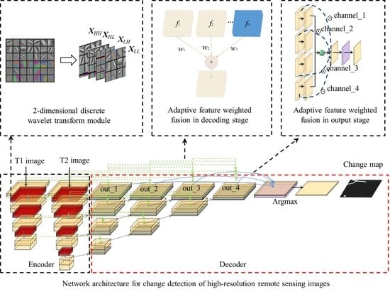
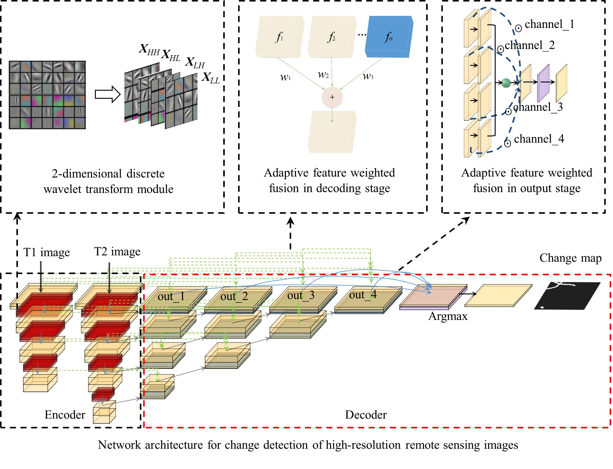
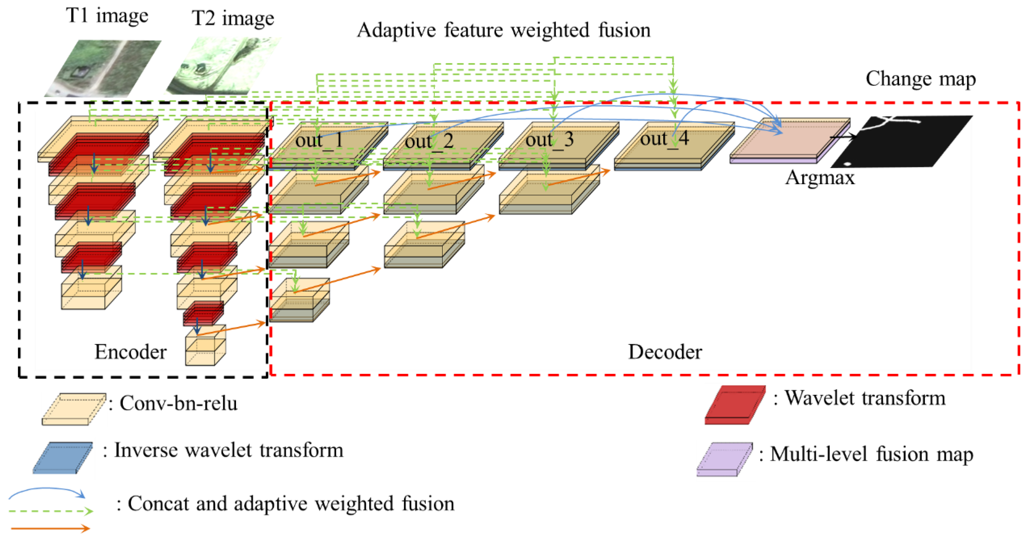
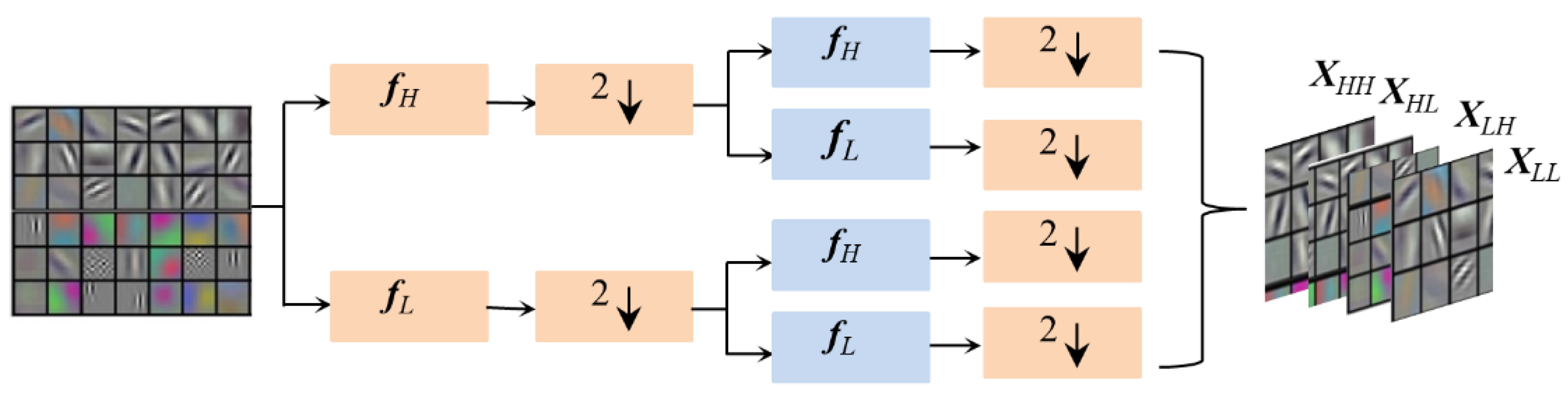
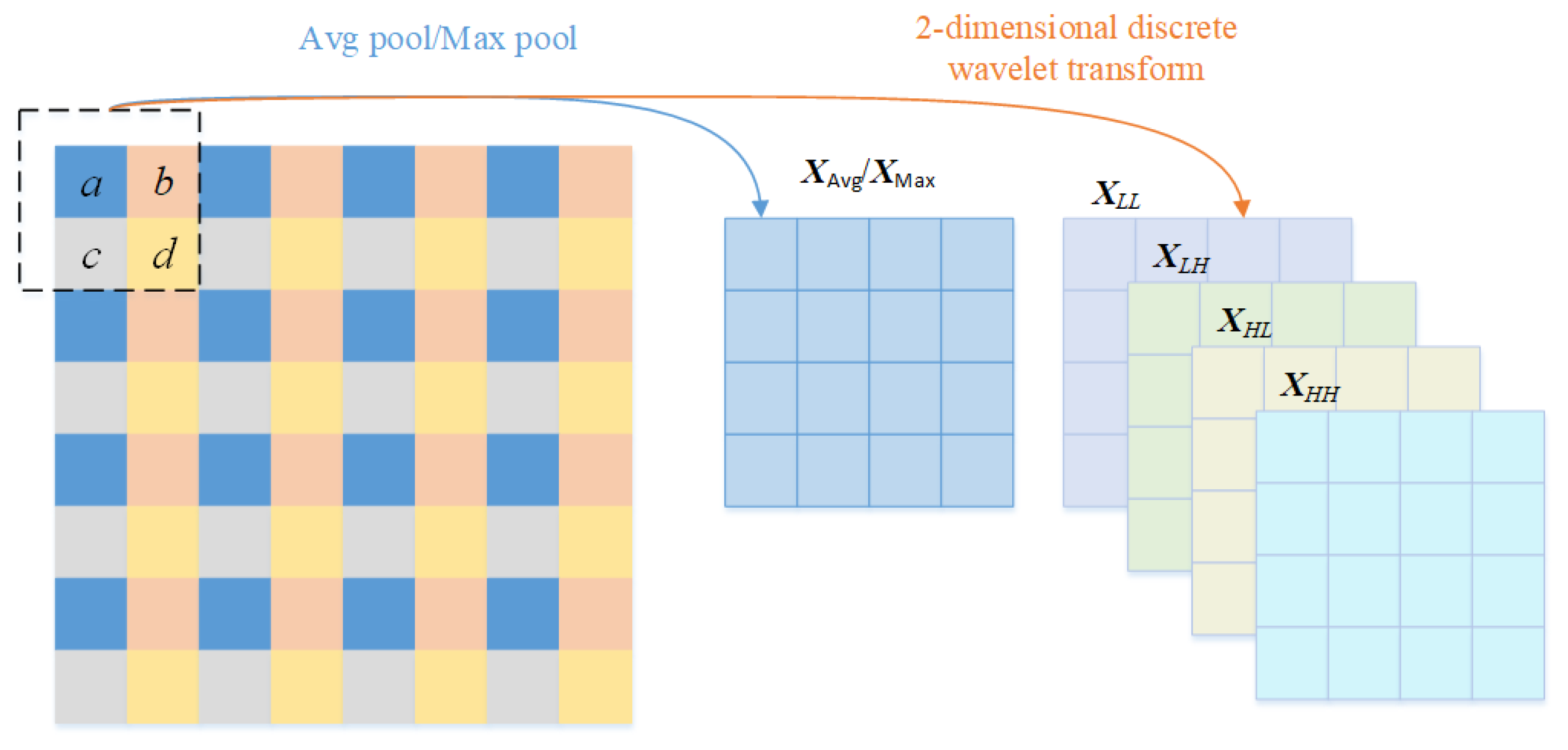
  • 2-dimensional discrete wavelet transform is introduced into the Nested U-Net, which can reduce the loss of spatial information resulting from pooling during encoding, and provide sufficient feature information for further change detection and change map reconstruction.
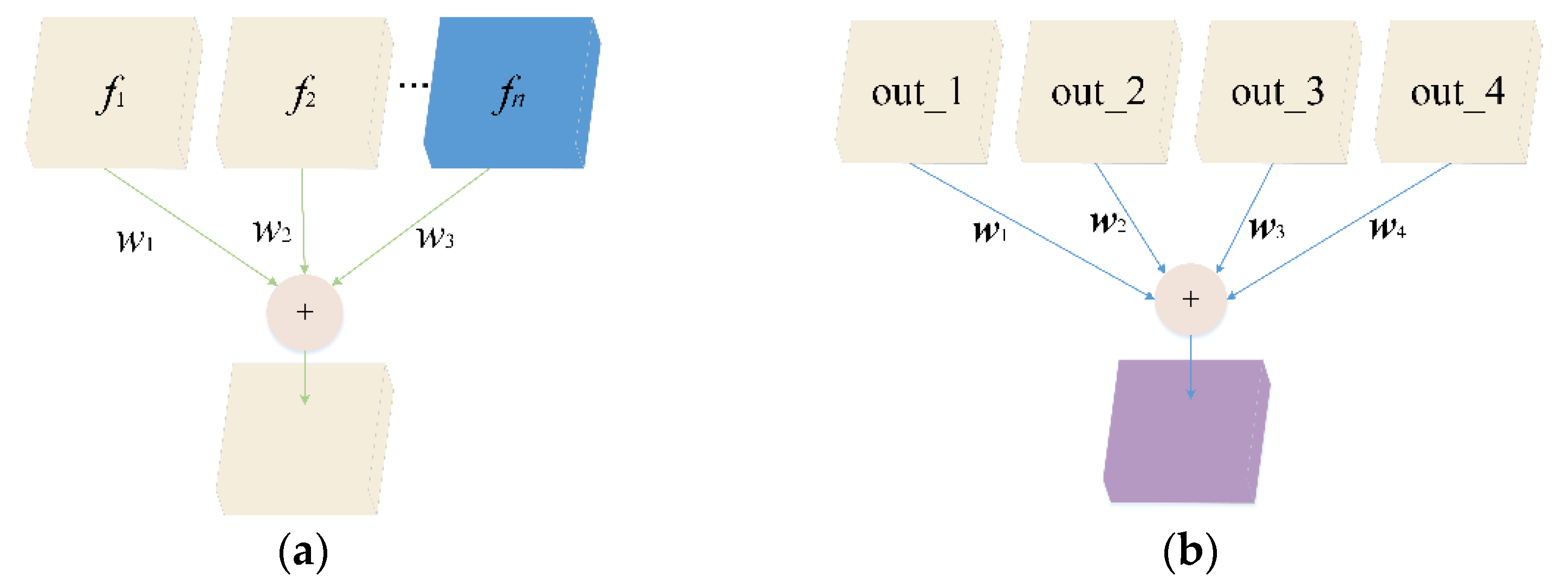
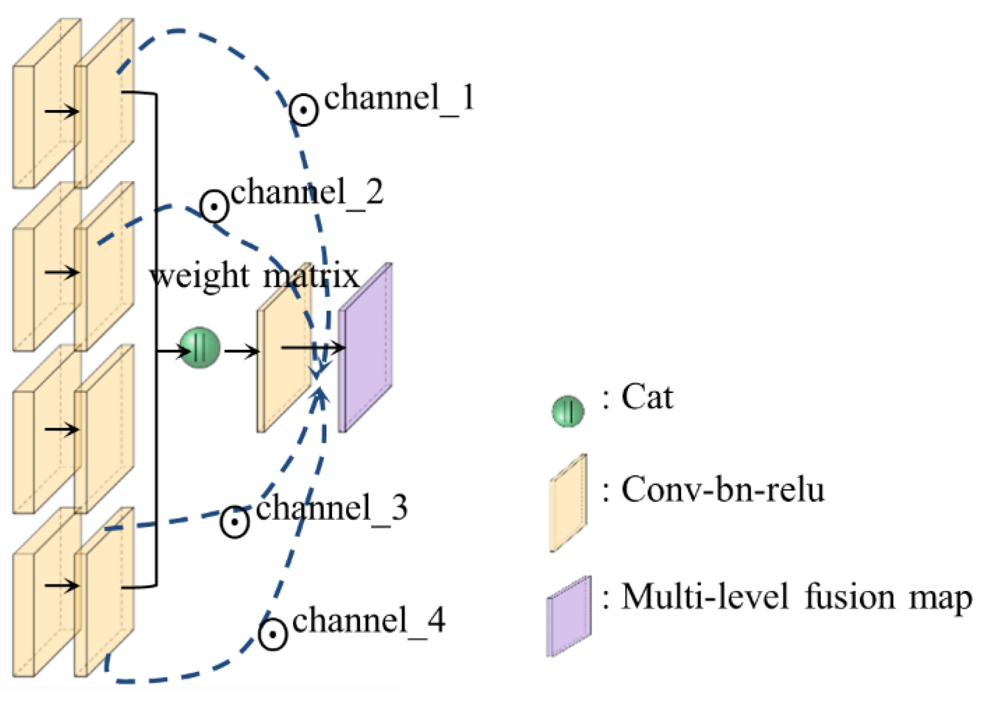
  • Adaptive weight parameters are calculated in different ways in the feature fusion of the decoding and output stages. Moreover, in the process of training, the relationship between the features is adaptively modeled, which improves the feature representation ability.
  • The comparative experiments with seven state-of-the-art methods on two change detection datasets show that the proposed method has better performance than other methods in detecting changed objects of different scales and positioning the boundary of changed objects.
The structural arrangement of paper is as follows. Existing deep learning methods for change detection of high-resolution remote sensing images are described in Section 2. Section 3 details the method proposed in this paper. In Section 4, the comparative experiments and ablation study are performed on two datasets to verify the effectiveness and advancement of our method, and the rationality and overall performance of the model are discussed in detail. Finally, the paper is summarized in Section 5.

2. Related Work

Enhancing the feature discrimination, fusing multi-scale and multi-level features, and improving the feature representation ability are the main ways for deep learning methods to improve the change detection performance. Therefore, existing change detection methods of deep learning are briefly introduced from the perspectives of enhancing feature discrimination and feature fusion.

2.1. Methods of Enhancing Feature Discrimination

Many methods improve the change detection performance by enhancing the discrimination of features; the main idea is to increase the inter-class distance between changed regions and reduce the intra-class distance between unchanged regions. Refs [27,28] constructed mapping relationship between unchanged regions by selecting reliable unchanged regions as training samples which were obtained from the generated coarse change maps. Finally, similarity analysis was performed on the mapped feature pairs to realize change detection. In [29], unchanged regions were selected as the training samples by preprocessing with the method of change vector analysis (CVA) and K-means. Then, they were projected into a high-dimensional space by using the FCN, before a projection matrix of the unchanged features was obtained by using the slow feature analysis. Finally, the extracted deep features were projected to the unchanged space using the projection matrix, and the change map was obtained by threshold segmentation. Xu et al. [11] used the capsule network as backbone, and improved the feature discrimination by reconstructing the unchanged regions and constraining the feature consistency between unchanged regions. However, the weakness of the above methods is that the threshold needs to be artificially determined. In addition, the GAN [30] is also widely used in change detection. Fang et al. [10] believed that the bi-temporal images were from different domains because of the different image acquisition conditions, and the change detection effect was not as good as the images in the same domain. Thus, bi-temporal images were transformed onto the same domain using the GAN. Then, image features were extracted using the FCN, and change maps were predicted by calculating the Euclidean distance between feature maps. In [31,32], the generator was used to predict the regions of changed, and then the generated change map was discriminated from the real change map, and the changed regions of the bi-temporal images were identified by training alternately. Although the GAN is able to make the task of change detection into a closed loop through alternating training of the generator and discriminator, the problem is that training GAN needs to achieve Nash equilibrium and gradient extinction may occur during training, causing the training to crash [33]. More importantly, the above methods which focus on the pseudo-changes in high-resolution remote sensing images change detection; thus, there are still some problems in the detection of small objects and the objects boundary positioning.

2.2. Methods of Feature Fusion

For deep learning-based change detection methods, the high-quality feature representation can improve the detection accuracy of changed objects of different scales while simultaneously reducing pseudo-changes. The feature fusion methods to fuse information from different features is an effective way to obtain high-quality features, which can be divided into image-level fusion and feature-level fusion. Among them, according to the data type and fusion stage, the image-level fusion method can be divided into heterogeneous fusion [34,35,36], early fusion [37], and late fusion [8]. On the other hand, in deep network, shallow features have high spatial resolution and sufficient geometric localization information, while deep features are more abstract and contain more context information due to the stacking of convolution and pooling, but a certain geometric localization information is lost [38,39]. The feature-level fusion method is used to integrate features which have high resolution and less semantic information with features which have low resolution and rich semantic information. Moreover, it can combine the advantages of the two types of features to reduce pseudo-changes and improve the detection accuracy of changed objects of different scales. In [40,41], the skip connection was used to connect the encoding and the decoding layer with the same resolution, which was expected to use the spatial information of shallow layer to compensate for the missing information of deep layer, so as to realize fine change detection. Hou et al. [9] used high-resolution networks (HRTNet) with parallel extraction of high-resolution features and low-resolution features to solve the problem that the deep features with low-resolution extracted from deep network lose the characteristics of high-resolution images, and fused features of different scales and levels using dynamic convolution. The proposed method reduced the loss of information resulting from pooling and partly enhanced the ability of feature representation. The densely connected Nested U-net was used as a backbone to fully fuse the features of different scales and levels, with improved performance in the detection of subtle changes [37]. In [17,42,43], dilated convolution was introduced to extract multi-scale features with different receptive domains, and the information from multi-level and multi-scale were fused to generate accurate change maps. Xu et al. [44] proposed that the one-way fusion flow hinders the feature expression, and proposed a feature fusion method of multi-directional which includes the direction of bottom-up, top-down, and shortcut-connection to improve the accuracy of change detection. In addition, the attention mechanism [45] can enhance useful information and suppress useless information, making it an effective method of feature fusion. An ensemble channel attention module was proposed in [46] to integrate different levels of semantic information, and realized the effective integration of multi-level channel features. A change detection method with dual attention mechanism was proposed in [47], which combined the channel and spatial attention mechanism, and made the extracted features more discriminative. Chen et al. [48] considered the temporal dimension of bi-temporal images and introduced the self-attention module into network to model the spatial-temporal relationship of bi-temporal images, effectively reducing the false detection due to registration errors and more refined change maps which were obtained. The loss of spatial information makes the accuracy of small objects change detection and boundary localization still relatively weak, even though the above feature fusion methods which fuse features of different levels and scales partly increase geometric localization information for deep features. Furthermore, the feature fusion methods, regardless of the relationship between features and fusion purposes, in some scenarios, increase the computational amount without significantly improving the ability of feature representation.
From the above review of deep learning-based change detection methods, we know that the methods of enhancing feature discrimination focus on improving the network robustness to pseudo-changes, while feature fusion methods which can improve the overall detection performance while reducing pseudo-changes are effective in change detection. However, the existing high-resolution remote sensing images change detection performance is still limited by the loss of spatial geometric information and insufficient feature representation caused by the deep network. Since the 2-dimensional discrete wavelet transform is able to decompose and accurately reconstruct the image, we consider introducing it into the network to solve the problem of spatial geometric information loss. On the other hand, starting from the network structure and feature characteristics, the adaptive feature weighted fusion is conducted in different weight calculation ways in different stages, so as to enhance the feature comprehensive representation ability and improve the identification rate of small objects in change detection. The methods of this paper are described in detail below.

3. Methodology

The proposed method is presented in detail in this section. First, Section 3.1 comprehensively describes the overall architecture of the network. The key parts of the proposed method, the 2-dimensional discrete wavelet transform module and the adaptive feature weighted fusion module, are elaborated in Section 3.2 and Section 3.3, respectively.

3.1. Network Architecture

The proposed network is based on the densely connected Nested U-Net. The difference is that, in our method, the encoder is a Siamese network with shared parameters, while using 2-dimensional discrete wavelet transform to reduce image spatial resolution instead of pooling, and the inverse transform to recover image spatial resolution instead of upsampling which can improve the model’s sensitivity to spatial location information. Furthermore, features are fused using the different feature weighted fusion methods at different stages to enhance the discrimination between unchanged and changed features. The overall network architecture is shown in Figure 1.
First, the bi-temporal images of T1 and T2 are used as the input of network, and feature extraction is performed using the encoder. The encoder mainly includes convolutional module and 2-dimensional discrete wavelet transform module. Additionally, the convolutional module consists of convolution, batch normalization, and activation. During the encoding process, the abstract features are first extracted using the convolutional module, and then are inputted to the 2-dimensional discrete wavelet transform module to reduce the image spatial resolution. The next convolution and 2-dimensional discrete wavelet transform are then performed. After encoding, decoding is performed to change detection. The decoder mainly includes convolutional module, 2-dimensional discrete wavelet inverse transform module, and adaptive feature weighted fusion module. During the decoding process, the inverse wavelet transform is used to recover the deep features with low spatial resolution to the same higher spatial resolution as the adjacent layer feature maps, and then the feature maps with the same spatial resolution (features obtained from 2-dimensional discrete wavelet inverse transform and features of the same level) are fused by the adaptive feature weighted fusion method of decoding. The out_1, out_2, out_3, and out_4 are the outputs of different levels, which are then fused by using the adaptive feature weighted fusion method which is different from the fusion method in the decoding process. Finally, the last convolution is performed, the operation of argmax determines whether each pixel changed, and then the change map is obtained.
As mentioned in the previous analysis, the pooling operation of the standard convolutional module in the classical convolutional neural network (CNN) can reduce the image spatial resolution and help to extract semantic information, but can also cause a certain loss of positional information. The 2-dimensional discrete wavelet transform module is designed to transform irreversible image downsampling into a reversible image decomposition so that the image spatial resolution reduced in the encoding stage can be accurately reconstructed in the decoding stage. In addition, the feature maps of different levels represent different feature information, and the feature fusion strategy can be used to fuse them to obtain features with rich spatial and semantic information. Therefore, it is possible to improve the recall and precision by adding the above two modules.

3.2. 2-Dimensional Discrete Wavelet Transform Module

The CNN architecture mainly includes the convolutional layer, the pooling layer, and the activation layer. The pooling layer can reduce the number of parameters and calculation amount by reducing the spatial information of image. More importantly, the operation of pooling enables the model to extract a larger range of features and increase the context information. In practice, this operation can obtain more context information by discarding the precise location of features which are important for high-resolution images change detection. The 2-dimensional discrete wavelet transform can decompose and accurately reconstruct the image, and the downsampling included in the decomposition process can also reduce the spatial resolution. Based on this, the decomposition and reconstruction of the 2-dimensional discrete wavelet transform which replaces the pooling and upsampling can not only reduce the loss of spatial information, but can also expand the receptive field and increase the context information that the pooling operation is expected to realize through downsampling.
The 2-dimensional discrete wavelet transform is essentially a kind of convolution, which can be naturally embedded into the neural network. For the input 2-dimensional image signal, the decomposition process is shown in Figure 2. First, along the image row direction, each row of the image is convolved with the low-pass filter and the high-pass filter to obtain the low-frequency component and the high-frequency component in the row direction. Then, low-frequency and high-frequency filtering is performed again on the column direction of the low-frequency component and the high-frequency component, and the obtained four sets of results are the decomposed images which contain all the image information. The reconstruction of the image is the inverse of decomposition, and the reconstructed image can be obtained by inverse transformation along the column and then along the row.
Different results can be obtained by performing 2-dimensional discrete wavelet transform with different wavelet bases on the image signal. In order to obtain a good transformation effect, an appropriate wavelet basis needs to be selected according to the properties of the wavelet basis and actual application requirements. Vanishing moment, compactly supported, orthogonality, symmetry, and regularity are the five important properties of the wavelet basis [49,50]. The vanishing moment is the wavelet order; the higher the vanishing moment, the more concentrated the energy after the wavelet transformation. It is worth mentioning that this will also cause a wider support width. The width of the wavelet basis is compactly supported. The shorter the support width, the stronger the localization ability of the wavelet basis and the higher the operational efficiency. Orthogonality ensures that there is no redundancy in the decomposition of the signal, which is conducive to the accurate reconstruction of wavelet coefficients. The symmetry of the wavelet basis ensures that it has a linear phase, which can avoid phase distortion during image reconstruction and make the reconstructed signal closer to the original signal. Regularity reflects the smoothness of the wavelet function, and the two are directly proportional. Furthermore, the better the regularity, the smaller the reconstruction error caused by quantization or truncation, and the better the image reconstruction effect. In most cases, the regularity of the wavelet basis increases with the increase in the vanishing moment. According to the above properties, from the perspective of image reconstruction effect and operational efficiency, since the Haar wavelet [51] has orthogonality, symmetry, certain regularity, and short support width, it is embedded in the network to perform the decomposition and reconstruction of the image.
For image decomposition, the filters are:
f L L = ( 1 1 1 1 )   f L H = ( 1 1 1 1 )   f H L = ( 1 1 1 1 )   f H H = ( 1 1 1 1 )
among them, L and H represent low frequency and high frequency, respectively. The decomposition results can be expressed as:
{ X L L = ( f L L X ) 2 X L H = ( f L H X ) 2 X H L = ( f H L X ) 2 X H H = ( f H H X ) 2
here, X is the feature of image, is the operation of convolution, and 2 represents two times downsampling.
The reconstruction with Haar wavelet can be expressed as:
X ( 2 i 1 , 2 j 1 ) = ( X L L ( i , j ) X L H ( i , j ) X H L ( i , j ) + X H H ( i , j ) ) / 4 X ( 2 i , 2 j 1 ) = ( X L L ( i , j ) X L H ( i , j ) + X H L ( i , j ) X H H ( i , j ) ) / 4 X ( 2 i 1 , 2 j ) = ( X L L ( i , j ) + X L H ( i , j ) X H L ( i , j ) X H H ( i , j ) ) / 4 X ( 2 i , 2 j ) = ( X L L ( i , j ) + X L H ( i , j ) + X H L ( i , j ) + X H H ( i , j ) ) / 4
where i and j, respectively, represent the pixel coordinates in the row and column direction.

3.3. Adaptive Feature Weighted Fusion Module

It is difficult to make full use of features and improve the feature expression ability for the fusion methods without considering the relationship between features and the purpose of fusion. On the one hand, feature fusion methods directly using the operation of concatenating or adding cannot reflect the importance of features, causing excessive attention to irrelevant information and neglect of important information. On the other hand, when the attention mechanisms with different structures are used for feature fusion, there are also some differences in performance. In order to address the above problems, the feature fusion methods of the decoding stage and the output stage introduced in Section 3.1 are designed separately. Furthermore, an adaptive weighted feature fusion module suitable for the two stages is proposed, aiming to fully combine the semantic and geometric features of multi-level and multi-scale feature maps to improve the model performance.
The feature fusion in the decoding stage is a kind of comprehensive expression of the features from different sources, while the feature fusion in the output stage is to fully integrate the semantic information of deep layers with the spatial geometric information of shallow layers, and improve the feature representation and geometric positioning ability of the model. According to the difference between them, different feature fusion methods are proposed, as shown in Figure 3.
Feature fusion in the decoding stage is achieved by weighting features from different sources. Taking Figure 3a as an example, the features to be fused include n − 1 convolutional feature maps and 1 upsampled feature map, and the fused features can be expressed as:
f f u s i o n = w 1 × f 1 + w 2 × f 2 + + w n × f n
w i = f r e l u ( w i ) i = 1 3 w i
where w i represents the weight of different source features, which is adjusted during training along with the model parameters. f i represents different feature maps, while f r e l u indicates that Relu is used to map the weight parameters between 0 and 1.
Feature fusion in the output stage is achieved by weighting the spatial positions of the output at different levels. Figure 4 shows the detailed process of weight calculation and feature fusion. The calculation process of the weight matrix is as follows. First, 1 × 1 convolution is performed on out_1, out_2, out_3, and out_4. Next, the obtained 4 sets of feature maps are concatenated along the channel, and the 1 × 1 convolution is performed again to obtain a matrix with 4 channels. Then, the weight matrix is obtained by normalization. In this way, the importance of spatial information of different level features is encoded in the weight matrix. The weight of different channels indicates the importance of the features from different levels at each spatial position. Respectively, multiply out_1, out_2, out_3, out_4, and the weight of the corresponding channel in the weight matrix, and add the corresponding elements to get the final fusion feature map. The calculation process can be formulated as:
W = f s o f t   max ( conv 1 × 1 [ conv 1 × 1 ( out _ 1 ) , conv 1 × 1 ( out _ 2 ) , conv 1 × 1 ( out _ 3 ) , conv 1 × 1 ( out _ 4 ) ] )
f f u s i o n = i = 1 4 out _ i W [ : , i 1 : i , : , : ]
where W R b * c * h * w represents the weight matrix with multiple channels; b is the batch size; c is the number of channels; and h and w are the height and width of the feature map, respectively. [ , ] represents the operation of feature concatenating along the channel. conv 1 × 1 means convolution of 1 × 1. The using purpose of f s o f t   max is to normalize the weight matrix, map the weight to (0,1), and normalize so that the sum equals 1. In addition, represents the element-wise multiplication.

4. Experiments and Discussion

To verify the effectiveness of the proposed method, our method and the seven state-of-the-art methods are tested on two publicly available datasets. Preliminary preparation for the experiment is presented in the first five sections, including the introduction of the two datasets, comparison methods, loss function, evaluation indices, and implementation settings. Section 4.6 elaborates and analyzes the experimental results, including the quantitative, qualitative analysis and efficiency comparison analysis of all methods on the two datasets. Then, the effectiveness of the 2-dimensional discrete wavelet transform module and the adaptive feature weighted fusion module are verified on the ablation study of the two datasets. Finally, Section 4.7 discusses the rationality and overall performance of the proposed method.

4.1. Datasets

To verify the effectiveness of our method in the change detection task for different change types, the Lebedev dataset [52] (with change objects of buildings, roads, and cars) and the SenseTime dataset [53] (which contains different types of land use conversion) are selected as experimental datasets. The first dataset of Lebedev is derived from Google Earth, including seven pairs of images with pixels of 4725 × 2700 and four pairs of images with pixels of 1900 × 1000 with significant seasonal change, and whose spatial resolution is from 100 cm/px to 3 cm/px. Furthermore, the corresponding labels are manually annotated. In the practical experiments, the data set is composed of 256 × 256 image blocks obtained by randomly rotating the original images and cropping them. Overall, the entire dataset contains 10,000 image pairs for training, 2998 image pairs for validation, and 3000 image pairs for testing. The second dataset of SenseTime which was adopted by the artificial intelligence remote sensing interpretation competition of SenseTime in 2020. Unlike the Lebedev dataset, the SenseTime dataset focuses on detecting changes among land use types, with a more complex texture information. In the dataset, the total number of samples labeled is 2968 pairs and the image size is 512 × 512, corresponding to the spatial resolution of 0.5 to 3 m. In practical experiments, 2968 image pairs are divided into training, validation, and test sets in a ratio of 8:1:1.

4.2. Comparison Methods

To verify the effectiveness of our method, it is compared with seven methods and described as follows:
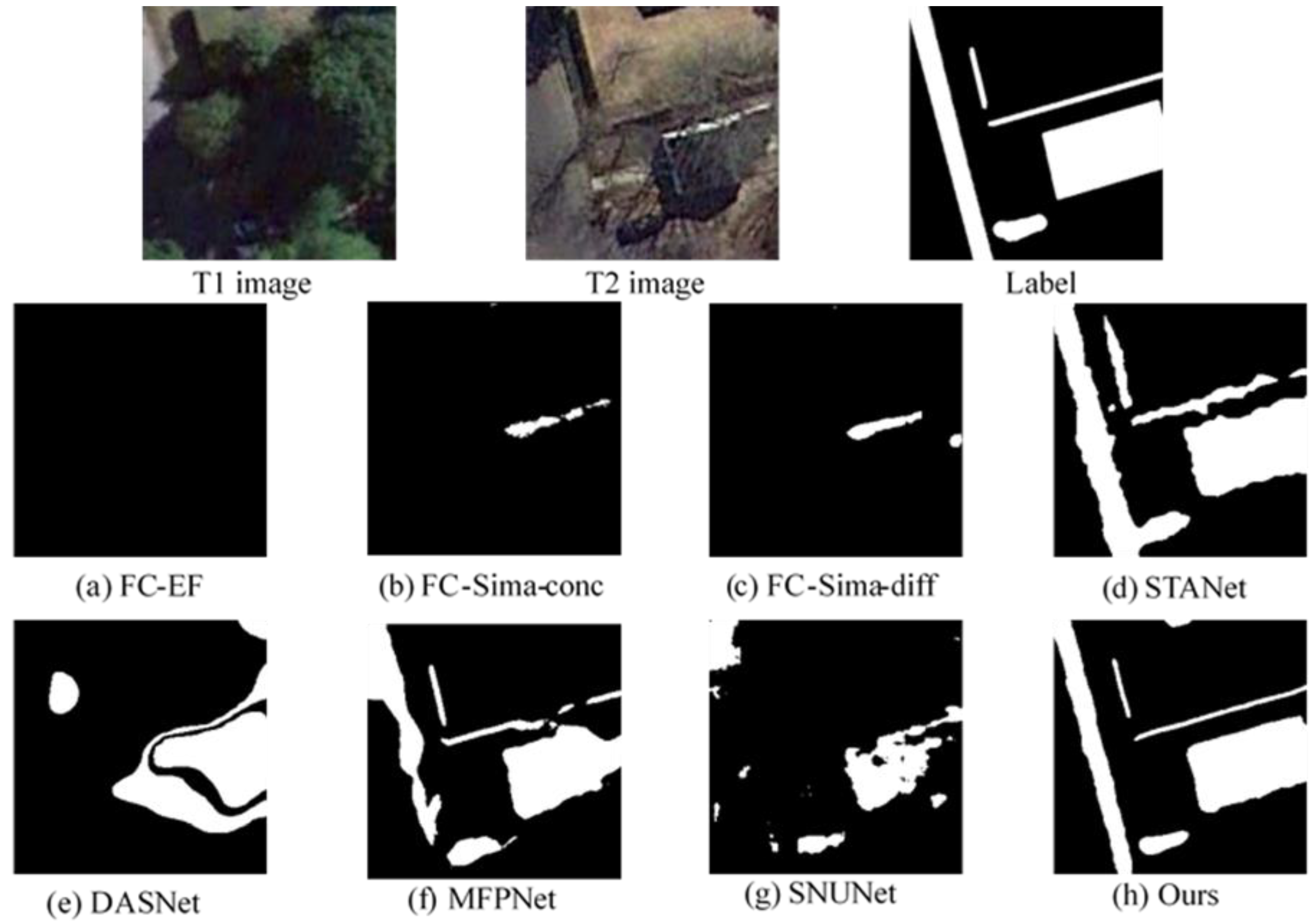
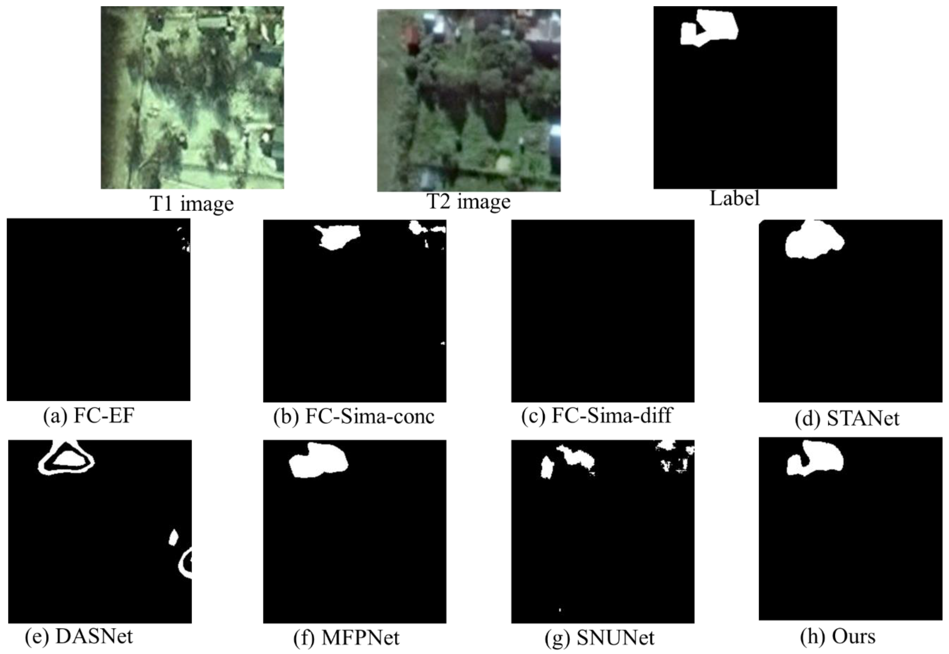
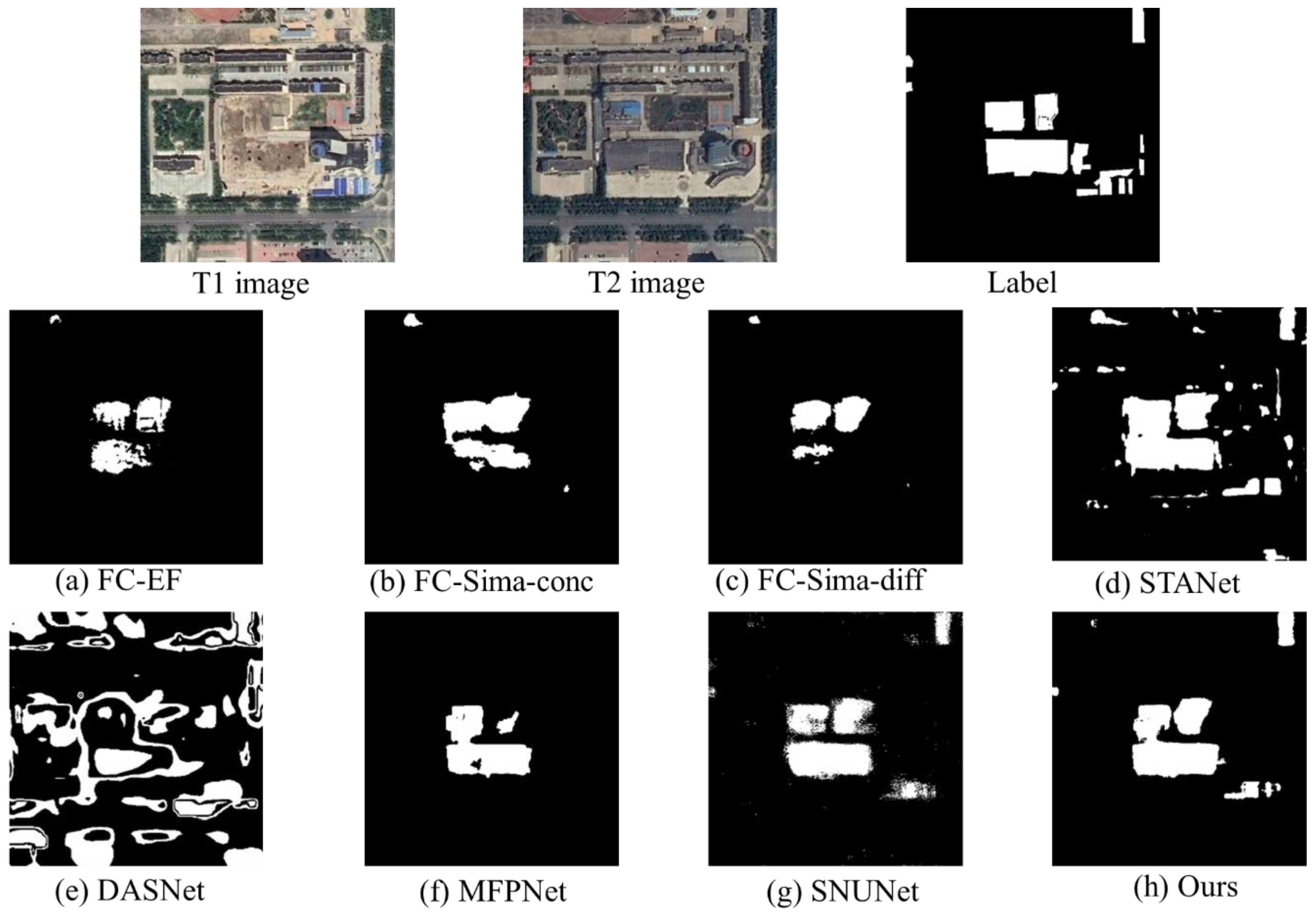
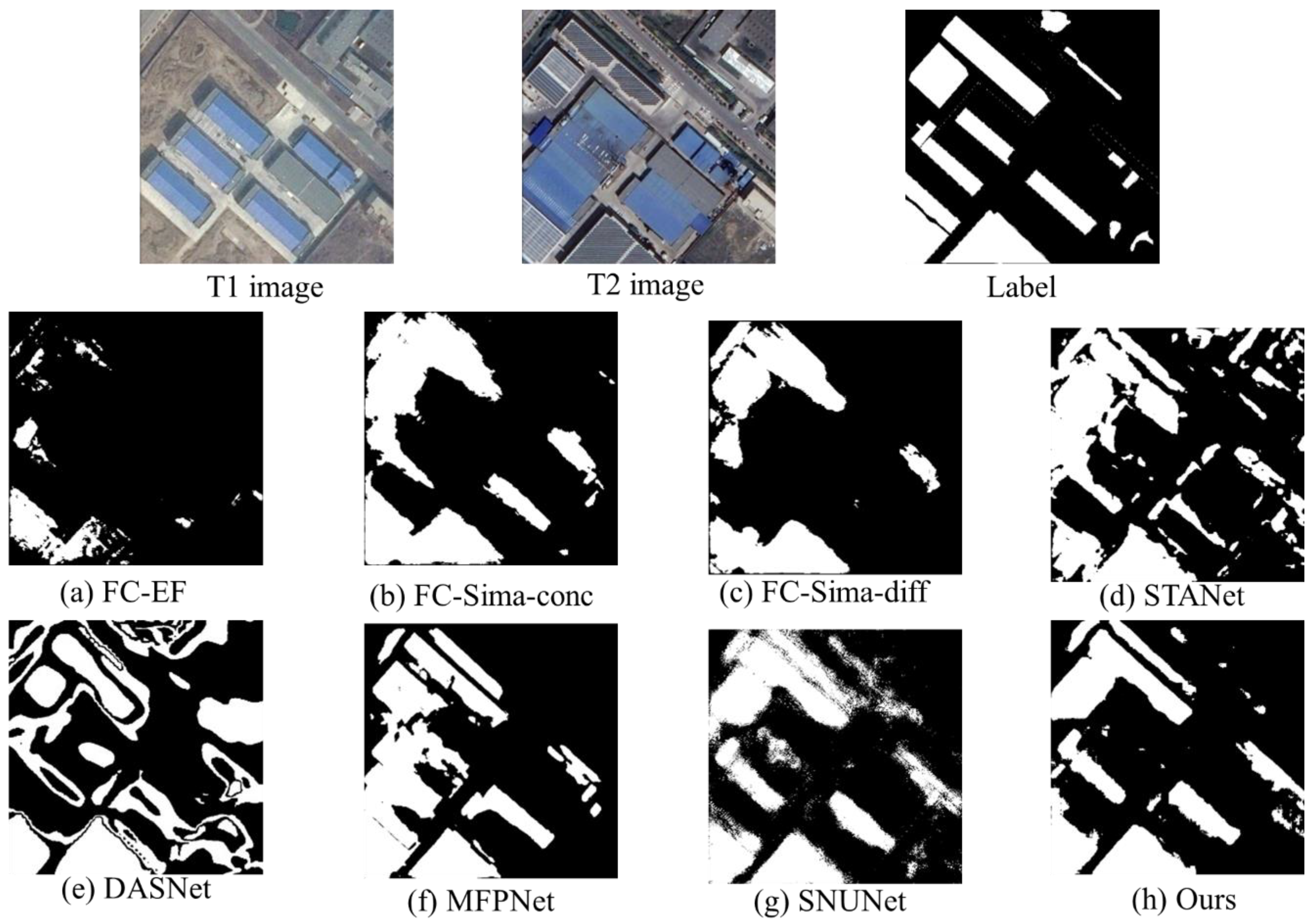
  • FC-EF [40]: The method of fully convolutional early fusion, which is an early fusion method in the level of image, takes U-Net as the backbone and concatenates bi-temporal images along the channel. Then, the images with six channels are inputted to network to train.
  • FC-Sima-conc [40]: The method of fully convolutional Siamese concatenation extends FC-EF to the Siamese network, and encodes bi-temporal images with shared weights. In the process of decoding, the feature-level fusion method is used to fuse the original encoded features and the joint encoded features of bi-temporal images in a directly connected manner.
  • FC-Sima-diff [40]: The fully convolutional Siamese difference method differs from FC-Sima-conc in the joint features of bi-temporal images are constructed in a differential manner rather than concatenation.
  • STANet [48]: STANet applies the self-attention mechanism to the network to extract the relationship with time dependence from bi-temporal images. Then, a pyramid spatial-temporal attention module is established to generate a multi-scale spatial-temporal attention map for multi-scale feature fusion.
  • DASNet [47]: The starting point of DASNet is to reduce the pseudo-changes in change detection of high-resolution remote sensing images. In the network, features are extracted in a Siamese network with weight sharing, and a dual attention that coupled channel attention and spatial attention is used to perform feature fusion, and the network is trained through metric learning.
  • MFPNet [44]: In the MFPNet, a method of multi-directional feature fusion combining bottom-up, top-down, and shortcut-connection is proposed, and features are fused by weighting features from different sources in an adaptive weighting manner. Then, a perceptual similarity module is proposed as a loss function for network training.
  • SNUNet [46]: SNUNet aims to improve the accuracy of small objects detection and objects boundary positioning in high-resolution remote sensing images change detection. It applies Nested-UNet to the Siamese network, and proposes an ensemble channel attention module to integrate the output feature maps of different levels, and finally achieves the balance of accuracy and efficiency.

4.3. Loss Function

The loss function can guide the direction of gradient descent and plays a vital role in the model optimization, and thus the selection of the loss function is crucial to the model training. The application scenario in this paper is change detection, which is essentially a binary classification problem with the categories of changed and unchanged, and binary cross entropy is a loss function commonly used in classification. While, unlike the classification, there is a proportional imbalance between the two categories, there are far more unchanged pixels than changed pixels in change detection. Dice loss [54] is able to effectively deal with the problem of data imbalance. Therefore, we combine the two loss functions as the total loss function, which can be expressed as:
L = L b c e log ( L d i c e )
where L b c e and L d i c e represent binary cross entropy loss and dice coefficient, respectively, and the dice coefficient takes the form of logarithm in order to put the two losses on the same scale. The two loss functions can be expressed as, respectively:
L b c e = ( y log ( y ^ ) + ( 1 y ) log ( 1 y ^ ) )
L d i c e = ( 2 y ^ y ) / ( y ^ + y )
where y [ 0 , 1 ] is the label, and 1 and 0 indicate the changed sample and the unchanged sample, respectively. y ^ represents the probability that the predicted sample is positive.

4.4. Evaluation Indices

In the task of change detection, we expect as many the predicted changed pixels as possible are really changed pixels (correctly found), and as many changed pixels as possible to be detected (all found). Based on the above, three indices of precision, recall, and F1-score(F1) are selected for quantitative evaluation.
Precision = TP TP + FP
Recall = TP TP + FN
F 1 = 2     Precision Recall Precision + Recall
where precision and recall are used to quantify the degree of “correctly found” and “all found”; and F1 is the harmonic mean of precision and recall, used for comprehensive evaluation. TP indicates that the prediction result is consistent with the label, which are changed pixels. TN means that they are all unchanged pixels. FP and FN indicate that the prediction results are different from the label, and the label corresponding to the two are unchanged pixels and changed pixels, respectively.

4.5. Implementation Settings

The experiments are implemented using pytorch as the framework on a workstation with CPU as Intel (R) Xeon (R) Gold 5118 CPU @ 2.30 GHz and a graphics card as NVIDIA Quadro P5000. In the experiments, the optimizer is AdamW, the initial learning rate is set to 0.001, and when the loss of the validation set does not decrease for five consecutive epochs, the learning rate is updated at a rate of 0.5. In the comparative experiments, for fair comparison, all methods are trained 100 epochs from scratch in the same computing environment.

4.6. Experiments Results

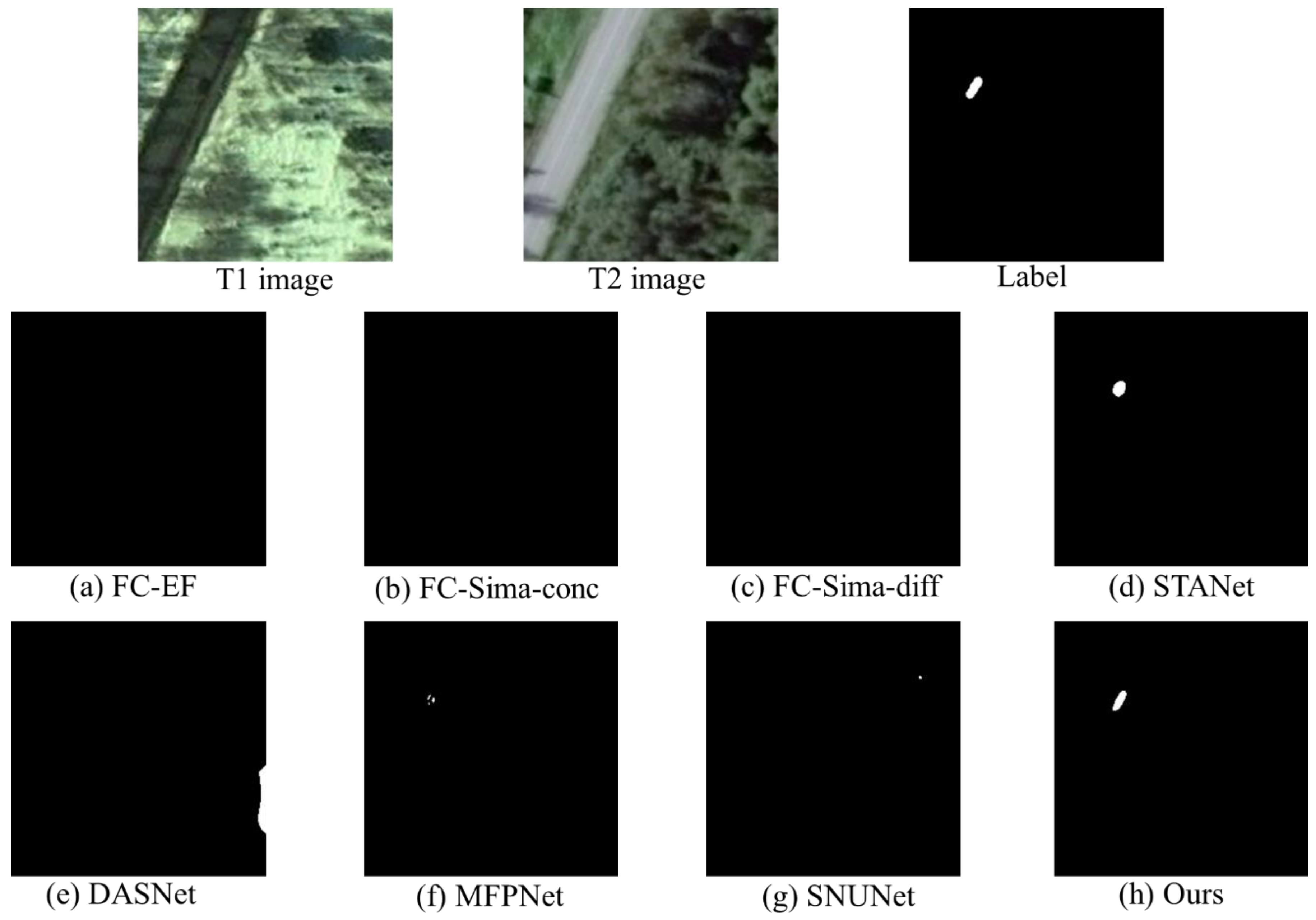
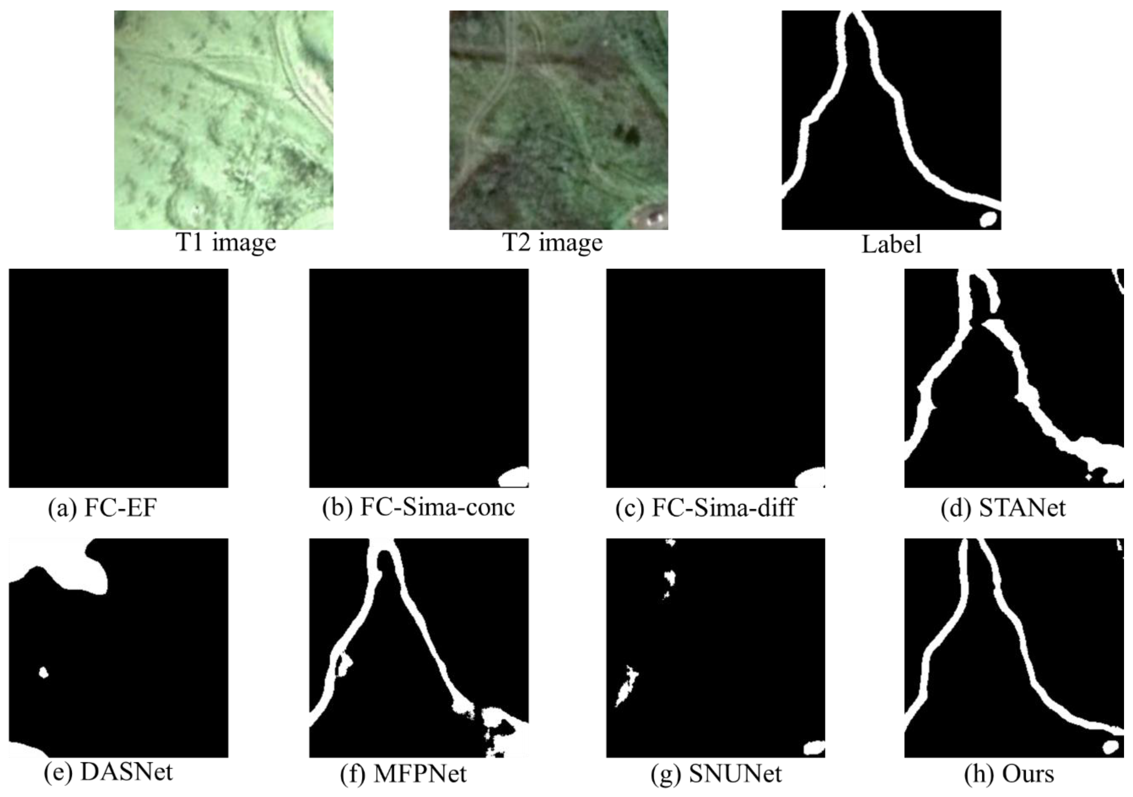
4.6.1. Performance Comparison on the Lebedev Dataset

Quantitative evaluation: The proposed method and comparison methods are tested in the same environment, and precision, recall, and F1 are used as evaluation indices. The experimental results are shown in Table 1, and the best results are shown in bold.
As seen from Table 1, our method has the best overall performance, with an F1 of 94.40%. The reason is that after two-stage adaptive feature weighted fusion, the extracted features have a stronger representation ability, and the changed and unchanged regions can be better distinguished. In particular, compared to the MFPNet, which has the sub-optimal overall performance, our method improves by 4.51% on recall. It suggests that, since the 2-dimensional discrete wavelet transform module adopted in the feature extraction stage retains more spatial information, more small objects and object boundaries can be detected. In addition, the STANet has the highest recall but has relatively low precision and brings out more false detections. Overall, our method achieves a good trade-off between precision and recall.
Qualitative evaluation: To validate the robustness of our method in different scenes, the experimental scenes are divided into five categories: large, medium, and small changed objects, as well as long and narrow changed objects with clear boundaries and complex scene. An image from each is selected, the experimental results of our method and comparison methods in five scenes are presented in the form of change map, as shown in Figure 5, Figure 6, Figure 7, Figure 8 and Figure 9.
Figure 5 shows the detection results of large changed objects. It can be seen that, in the bi-temporal images, the change of the tree caused by seasonal change is more obvious than those of roads and buildings, while the goal of change detection is to identify changed roads and buildings instead of the tree. The FC-EF fails to identify changed roads and buildings under the influence of seasonal changes due to the weak feature representation capability. Furthermore, the FC-Sima-conc and FC-Sima-diff have improved performance compared to the FC-EF, but they also identify only a small number of changed samples. The changed regions detected by the DASNet are inconsistent inside, and there are many samples were not detected. Although the MFPNet can roughly locate the changed regions, the overall detection effect is slightly poor. Specifically, the detected roads are distorted and the buildings are incomplete. Our method and the STANet are the best, but there are burrs on the boundaries of the changed objects detected by the STANet, which makes the change map rough. In contrast, our result has clearer boundaries and is closer to the label. The reason is that the 2-dimensional discrete wavelet transform module in the proposed network can fully retain the original image information, so that the extracted features have more abundant spatial location information.
Figure 6 shows the detection results of medium changed objects. All the methods, except the FC-EF and the FC-Sima-diff, could not identify the changed regions, while other methods can roughly determine the range of changed regions. However, judging from the detection accuracy and the boundary details of the change map, the detection result of our method is the closest to the label, followed by the MFPNet and the STANet. The specific performance of our method is superior to the other two methods of accurately identifying the interval between buildings and better distinguishing the changed regions from unchanged regions.
Figure 7 shows the detection results of small changed objects. It can be seen from the figure that the object is too small for humans to recognize it under the influence of seasonal changes. However, the STANet and our method can roughly locate the changed region, while no other method can identify the object under the influence of pseudo-changes. In the above two methods, the changed region of the STANet is significantly larger than the label, and parts of the unchanged regions are mistakenly identified as changed regions. Since our method retains more spatial location information during the feature extraction process, changed objects with small scale can be accurately detected and located.
Figure 8 shows the detection results of a long and narrow changed object, and our method can obtain a change map with an accurate regional shape. The MFPNet and the STANet can also obtain good detection results, but compared with our method, the false positive predictions of the STANet expand the boundary range and significant missed and false detections appear in the lower right corner of the change map. Furthermore, the boundary of the MFPNet is better than the STANet, but the road is broken in the lower right corner of the change map and there are some wrong distinctions between the changed and unchanged regions.
Figure 9 shows the change detection results of a complex scene and that our method and the STANet can better distinguish changed regions from unchanged regions. While, in contrast, the gap formed by the change regions in the unchanged regions in the upper left corner of the label is not shown in the result of the STANet, and the right boundaries are discontinuous in the change map of the STANet. Our method can effectively distinguish real changes from pseudo-changes, while obtaining the change map with refined boundaries. The reason is that the adaptive feature weighted fusion method and 2-dimensional discrete wavelet transform can extract features with stronger representation ability and richer spatial information. Although the MFPNet can identify most of the changed regions, it cannot avoid the influence of pseudo-changes, resulting in many false detections. In addition, the other methods are not effective.
The results of Figure 5, Figure 6, Figure 7, Figure 8 and Figure 9 show that, in the change detection of different scenes, compared with other methods, our method can retain more spatial information and the change detection results are more refined. Specifically, it is able to improve the detection accuracy of small objects while reducing the pseudo-changes caused by season and light, and return the change map with clear boundaries. As shown in the figures, there are still false detections, missed detections, and incomplete boundaries in some complex regions. The reason is that the training of the model is completed on the training set, and when tested using the test set, there are missed or false detections of difficult-to-detect samples due to the limitation of the model generalization ability. However, the overall detection effect is better than other methods.
Efficiency analysis: Considering the limitation of hardware computing power and the requirement of computing efficiency in practical applications, the number of parameter and the training speed of our method are compared with other methods. The parameter amount (take M as the unit) and the training time of an epoch (take min/epoch as the unit) are used as quantitative indicators for evaluation. The result is shown in Figure 10.
In the previous analysis, the STANet, MFPNet, and our method outperform other methods in change detection. However, it can be seen from Figure 10 that the MFPNet has the largest number of parameters, and it takes the longest time to train an epoch, followed by the DASNet and STANet, with some limitations in practical applications. Compared with the STANet and MFPNet, the parameter amount of our method is reduced by 15.53% and 76.40%, and the training time is reduced by 11.57% and 72.04%, respectively, making our method more available in practical applications. The FC series methods have the minimum number of parameters and training time, but from the quantitative analysis and qualitative analysis of the previous change detection results, the detection effect is not as good as other methods. The above facts show that our method obtains the optimal detection results while ensuring the efficiency, and has a good trade-off between accuracy and efficiency.

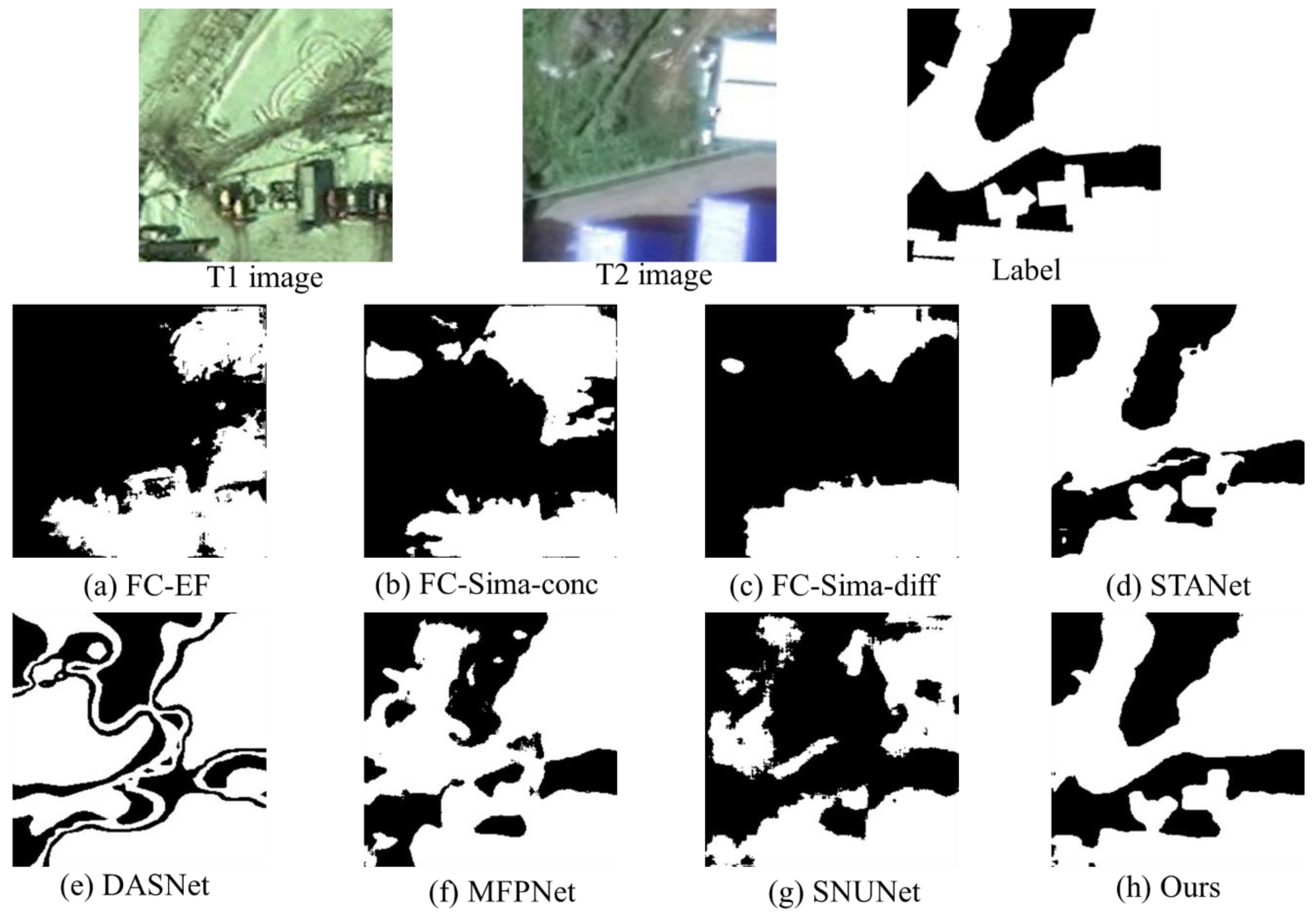
4.6.2. Performance Comparison on the SenseTime Dataset

Quantitative evaluation: The quantification results of our method and comparison methods on the SenseTime dataset are shown in Table 2.
As can be seen from Table 2, our method performs best comprehensively, with the F1 increased by 5.49% compared to the suboptimal STANet. The FC-EF, which has the simplest network structure, performs the worst overall, with a F1 of 45.56%. The performance is significantly improved as the FC-Sima-conc and FC-Sima-diff add the combined information of bi-temporal images on the basis of the FC-EF. Specifically, the F1 increased by 7.51% and 4.49%, respectively. Other methods have similar performance, where the method of STANet has the highest recall, but its precision is the lowest, leading to more false detections. In addition, the precision of the MFPNet is close to our method, but the recall is relatively weak, and it is difficult to achieve a great trade-off between precision and recall. Furthermore, compared with Table 1, it can be seen that the detection effect on the SenseTime dataset is not as good as that on the Lebedev dataset. The reason is that, firstly, the number of training samples in the SenseTime dataset is much smaller than the Lebedev dataset, and the performance of the deep learning model is largely related to the sample size. Second, training on the SenseTime dataset is to identify changes in different land use types, which performed more varied and complex on images, making it difficult for the network to train.
Qualitative evaluation: To verify the effectiveness of our method for different change scenes, two from the test set are selected as experimental scenes, and the detection results of the different methods are analyzed qualitatively, as shown in Figure 11 and Figure 12.
As seen from Figure 11 and Figure 12, there are many missed detections in the results of the FC-EF, because the extracted feature information is insufficient with the basic structure of encoder–decoder. The FC-Siam-conc and FC-Siam-diff incorporate combined information of bi-temporal images to each layer of the decoder, making significant improvements in the recognition rate and recognition accuracy of changed objects. The STANet, consistent with the results in the previous quantitative analysis, is able to detect more regions of change, but also increases the proportion of false detection, identifying partially unchanged regions as changed. Compared with the label, the detection result of DASNet has more holes, and there are relatively more missed and false detections. The SNUNet, MFPNet, and our method obtained better results. However, the SNUNet misidentifies partial changed samples within the changed regions as unchanged, making the change results incomplete. The detection results of the MFPNet are better than the SNUNet, but it is still slightly inferior to our method in detecting small objects and distinguishing between changed and unchanged regions. There are still missed and false detections and the change map boundaries are inconsistent with the label. This is mainly because, in the case of an insufficient sample size, the model has an insufficient representation of the features of some difficult-to-detect samples, making it difficult to obtain the correct prediction results. Moreover, due to the weak regularity of the Haar wavelet, the errors generated in the image reconstruction process may also cause prediction errors. Overall, compared with other methods, our detection results are closer to the label, showing optimal performance in the detection and localization of objects at different scales.

4.6.3. Ablation Study

To verify the effectiveness of the proposed method, the ablation study is performed on the two datasets, examining the effect of the 2-dimensional discrete wavelet transform module and the adaptive feature weighted fusion module on the model performance.
Verification of 2-dimensional discrete wavelet transform. This module replaces pooling and upsampling in the classical CNN architecture with 2-dimensional Haar wavelet transform and the inverse transform, respectively. To verify the effect of this module, the pooling layer in the encoding is set to the max pool and the avg pool, while the upsampling in decoding is realized by deconvolution, and the rest of the network is consistent with the original setting. The architecture of baseline is the Nested U-Net without adding the 2-dimensional discrete wavelet transform module and the adaptive feature weighted fusion module. The results are shown in Table 3.
As shown in the table, the model with 2-dimensional discrete wavelet transform module improves 3.96% and 2.92% on recall, and 3.28% and 1.9% on F1 on the Lebedev dataset, compared to the two models which use the operation of maxpool and avgpool to downsample. Similarly, on the SenseTime dataset, recall increased by 1.91% and 1.8%, and F1 increased by 3.78% and 3.02%, respectively. It is shown that the 2-dimensional discrete wavelet transform module can reduce the impact of spatial information loss and retain more feature information, significantly improving recall and the overall performance of change detection.
To explore the applicability and validity of the 2-dimensional discrete wavelet transform module on other architectures, we apply it to the FC-Sima-conc and the FC-Sima-diff. The experimental results are shown in Table 4.
As seen from Table 4, the recall and F1 of both methods are significantly improved after the addition of the 2-dimensional discrete wavelet transform module. This, again, confirms that the 2-dimensional discrete wavelet transform module is effective for reducing information loss. Furthermore, it also indicates model’s portability.
Verification of adaptive feature weighted fusion. The proposed adaptive feature weighted fusion method integrates the features from different sources and different levels in the decoding and output stages to improve the comprehensive representation ability of the features. To quantify the role of the proposed feature fusion method, the two stages of feature fusion in the original model are removed separately. The baseline architecture is the same as previously mentioned. These results are shown in Table 5.
It can be seen from Table 5 that, on the Lebedev dataset, compared with the results without weighted feature fusion, the models that only feature weighted in the decoding stage and the output stage improves the performance of 1.56%, 0.48%, and 0.99%, and 1.25%, 0.95%, and 1.08% in precision, recall, and F1, respectively. Similarly, on the SenseTime dataset, precision, recall, and F1 are improved, by 2.05%, 0.09%, and 1.59%, and 1.01%, 1.55%, and 1.45%, respectively. Furthermore, compared with the results of our complete network structure, it can be seen that performing feature fusion in two stages at the same time has better performance than using only a single stage of feature fusion. Specifically, it shows that, compared to model without feature fusion, the precision, recall, and F1 are, respectively, improved by 1.97%, 2.2%, and 2.09% on the Lebedev dataset, and 2.84%, 2.33%, and 3.2% on the SenseTime dataset with our method. Meanwhile, the results compared to baseline also demonstrate the effectiveness of our method. The above facts show that the feature fusion method proposed in this paper can fully combine the advantages of features and enhance the ability of feature representation so that the truly changed objects can be more detected and the changed objects detected are more truly changed objects.
Similarly, we perform adaptive feature weighted fusion on the FC-Sima-conc and the FC-Sima-diff to verify the applicability of the module in other network architectures. Since the network architectures of these two methods are different from ours, feature fusion can only be performed in the decoding stage in the experiment. The experimental results are shown in Table 6.
Available from Table 6, the precision, recall, and F1 of both methods improved significantly after the addition of the adaptive feature weighted fusion module. This suggests that simple feature concatenation or subtraction is insufficient for feature fusion, and our method can combine features more effectively.

4.7. Discussion

4.7.1. Analysis of Module Rationality

The rationality of 2-dimensional discrete wavelet transform. The 2-dimensional discrete wavelet transform module, which exists as an alternative operation to pooling in the classical CNN architecture, is related to the pooling operation, and there are some differences between them. To visualize the relationship between them, the 2-dimensional Haar wavelet transform given by Equation (2) is expressed in a clearer way:
{ X L L = ( a + b + c + d ) / 2 X L H = ( a b + c + d ) / 2 X H L = ( a + b c + d ) / 2 X H H = ( a b c + d ) / 2
And the operation of avg pool and max pool can be expressed as:
{ X avg = ( a + b + c + d ) / 4 X max = Max ( a , b , c , d )
where a, b, c, and d are the pixel values of the corresponding positions. Furthermore, the downsampling of the 2-dimensional discrete wavelet transform module and the avg pool and max pool can be represented in Figure 13.
From Equations (14) and (15), X avg is formally consistent with X L L , equivalent to a sub-feature of the 2-dimensional discrete wavelet transform. Due to the different normalization factors, the feature properties are not affected. Furthermore, X max can only obtain the features with the largest pixel value, and may lose other important features. It is worth noting that, as shown in Figure 13, the 2-dimensional Haar wavelet transform and avg pool and max pool can be expressed as a filter with a kernel size of 2 to convolve the image with a step size of 2. What the two kinds of methods have in common is that they both perform downsampling during the convolution, which enlarges the receptive field with the same proportion and adds contextual information. The difference is that both avg pool and max pool can only get one kind of feature, while the 2-dimensional Haar wavelet transform can get four kinds of features, which makes it more informative compared to pooling. Therefore, the addition of a 2-dimensional discrete wavelet transform module to the network can reduce the feature loss, while increasing contextual information and facilitate the recovery of image information in the decoding stage. The improvement of the recall in the ablation study of the 2-dimensional discrete wavelet transform also confirms that the above analysis is reasonable.
The rationality of adaptive feature weighted fusion. Feature fusion can combine the features with different properties, strengthen the effective features, and realize the improvement of the feature comprehensive representation ability. The adaptive feature weighted fusion module proposed in this paper is a feature fusion method of incorporating prior knowledge, guided by the relationship between features and the purpose of feature fusion. The main difference among the features to be fused in the decoding stage is their different sources, including the features obtained by the 2-dimensional discrete wavelet inverse transform, the encoded features, as well as the fused features. Thus, weighting features from different sources is a natural idea. Moreover, the main difference among the features of the output stage is that they come from different levels, and the spatial and semantic information of them are quite different due to different network depths. However, in the change detection task, the semantic information contributes to the identification of the regions of change, while the spatial information is crucial to the positioning of the regions of change. Weighting the spatial position of the output results at different levels can effectively combine the semantic and spatial information of the features. The ablation study shows that the feature fusion method in both stages can improve model performance and it is better to use both at the same time.

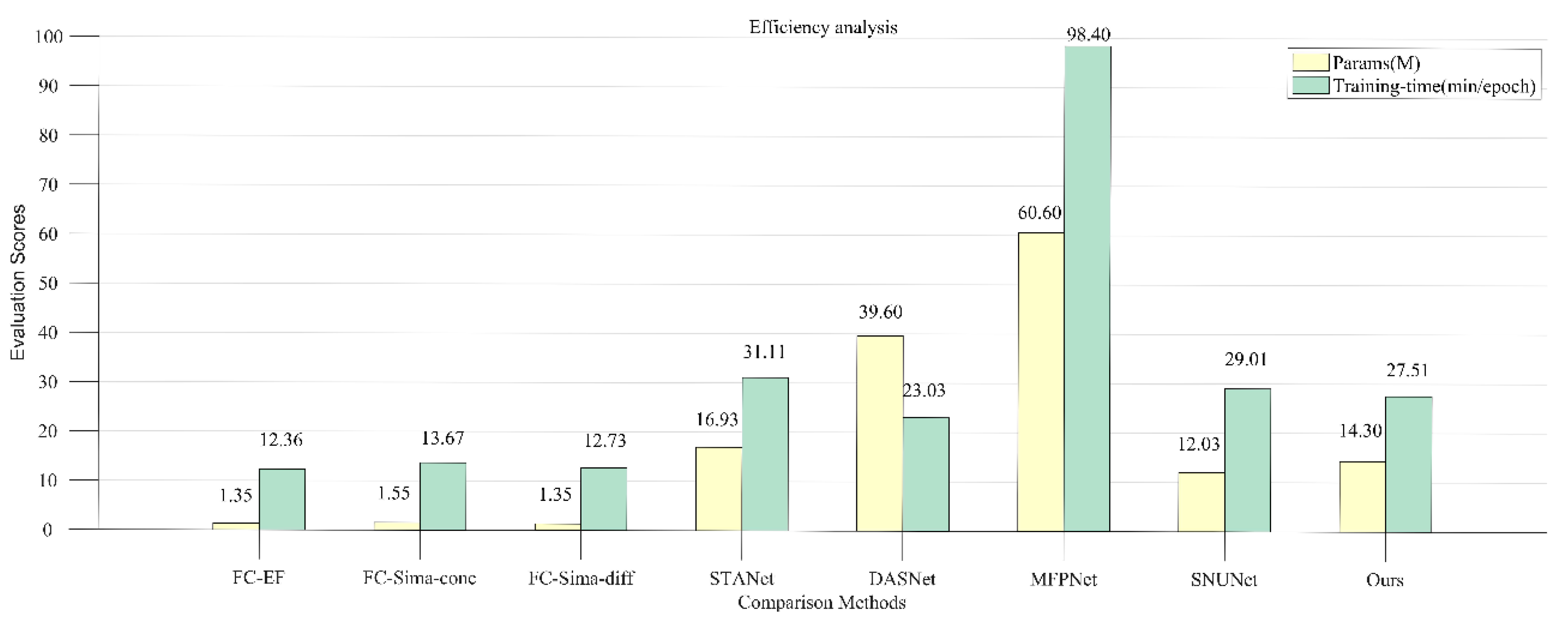
4.7.2. Analysis of Overall Performance

The results of experiment confirm the effectiveness of the proposed network architecture. The quantitative results show that, compared with other methods, our method can improve the recall and achieve the optimal effect while ensuring the precision on both datasets. This indicates that our model can exploit more image information and have more powerful feature extraction ability.
The qualitative results show that, in experiments with different scenarios, the FC series methods are inferior to other methods due to the simple network structure. The SNUNet performs better in both datasets compared to the FC series methods, suggesting that the densely connected network structure contributes to improving accuracy. There are some holes in the change map of DASNet, which makes the change regions broken and the internal compactness poor. Although the STANet and MFPNet can get good results on the two datasets, it can be seen from the results of small changed objects and complex scenes in the experimental scenes that their detection sensitivity to small objects and boundary positioning accuracy are both not as good as our method. Meanwhile, the results of the Lebedev dataset show that our method is robust to noise and can accurately identify real changes under the influence of pseudo-changes. Additionally, the results of the SenseTime dataset further validate the robustness of our method to different scenes and different change types. It is worth mentioning that our method can perform well in the quantitative and qualitative analysis, mainly due to the following aspects. First, we take the densely connected Nested U-Net as the backbone, which can reduce the semantic gap between the features of different levels and enhance the feature representation ability. Second, the proposed 2-dimensional discrete wavelet transform can capture more feature information during downsampling and reduce the information loss in the deep network. Third, the adaptive feature weighted fusion module can more efficiently combine the features, making the model focuses on useful information and further improving the model to identify changed regions. Finally, the adopted loss function can effectively guide the model learning and improve the overall performance of the model.
Efficiency analysis shows that, for our model on the Lebedev dataset, the parameter amount is 14.3 M and the time required for training an epoch is 27.51 min, which are far smaller than the most complex MFPNet with 60.6 M and 98.4 min. It is shown that the network architecture proposed in this paper has higher availability in practical applications, and can take into consideration operation efficiency and accuracy.
The above analysis shows that our method can be more widely used in change detection scenarios with higher requirements on small objects detection and boundary positioning, and does not require excessive hardware configuration.

5. Conclusions

In this paper, we propose an adaptive feature weighted fusion network based on 2-dimensional discrete wavelet transform from the perspective of reducing spatial geometric information loss and enhancing feature comprehensive representation capability for high-resolution remote sensing images change detection. Among them, embedding the 2-dimensional Haar wavelet transform and the inverse transform in the network can retain more spatial geometric information, make the feature information of small objects and object boundaries more sufficient, and contribute to the reconstruction of more refined change map. In addition, the two-stage feature fusion guided by feature relationship and fusion purpose can improve the feature representation ability and further improve the robustness of the model to pseudo-changes and the ability to detect changed regions.
Experimental results on publicly available datasets show that our method achieves optimal results on the Lebedev dataset with obvious seasonal variation and SenseTime dataset with complex image texture, with F1 of 94.40% and 68.67%, respectively. It is worth noting that, in experimental scenarios with different changed object scales and complexity, detection results with high internal compactness and clear boundaries can be obtained with our method. Furthermore, the detection effect of small objects is also better than other methods. From the perspective of operation efficiency, compared to other methods, the parameter amount and the training time of our method decreased by up to 76.4% and 72.04%, respectively. The above shows that our method can improve the overall performance of change detection while considering the efficiency, which is feasible in the task of change detection. However, our method has some limitations under small size of samples; thus, subsequent work should focus on few-shot learning about change detection.

Author Contributions

Conceptualization, C.W. and W.S.; methodology, C.W. and X.L.; software, C.W.; validation, W.S. and D.F.; formal analysis, C.W.; investigation, W.S. and X.L.; resources, Z.Z.; data curation, D.F. and Z.Z.; writing—original draft preparation, C.W.; writing—review and editing, W.S.; visualization, C.W.; supervision, C.W. and X.L.; project administration, C.W.; funding acquisition, W.S. All authors have read and agreed to the published version of the manuscript.

Funding

This research was funded by the Key Program of National Natural Science Foundation of China (Grant No. 41930650).

Institutional Review Board Statement

Not applicable.

Informed Consent Statement

Not applicable.

Data Availability Statement

The dataset of Lebedev and SenseTime are openly available at https://drive.google.com/file/d/1GX656JqqOyBi_Ef0w65kDGVto-nHrNs9 (accessed on 1 June 2018), https://aistudio.baidu.com/aistudio/datasetdetail/53484 (accessed on 4 April 2021).

Acknowledgments

We sincerely appreciate the editors and reviewers give their helpful comments and constructive suggestions. In addition, we also thank other researchers for creating and providing publicly available datasets.

Conflicts of Interest

The authors declare no conflict of interest.

References

  1. Xu, Y.; Yu, L.; Zhao, F.R.; Cai, X.; Zhao, J.; Lu, H.; Gong, P. Tracking annual cropland changes from 1984 to 2016 using time-series Landsat images with a change-detection and post-classification approach: Experiments from three sites in Africa. Remote Sens. Environ. 2018, 218, 13–31. [Google Scholar] [CrossRef]
  2. Rahnama, M.R. Forecasting land-use changes in Mashhad Metropolitan area using Cellular Automata and Markov chain model for 2016–2030. Sustain. Cities Soc. 2021, 64, 102548. [Google Scholar] [CrossRef]
  3. Nemmour, H.; Chibani, Y. Multiple support vector machines for land cover change detection: An application for mapping urban extensions. ISPRS J. Photogramm. Remote Sens. 2006, 61, 125–133. [Google Scholar] [CrossRef]
  4. Raja, R.A.A.; Anand, V.; Kumar, A.S.; Maithani, S.; Kumar, V.A. Wavelet Based Post Classification Change Detection Technique for Urban Growth Monitoring. J. Indian Soc. Remote Sens. 2012, 41, 35–43. [Google Scholar] [CrossRef]
  5. Papadomanolaki, M.; Verma, S.; Vakalopoulou, M.; Gupta, S.; Karantzalos, K. Detecting urban changes with recurrent neural networks from multitemporal Sentinel-2 data. In Proceedings of the IGARSS 2019–2019 IEEE International Geoscience and Remote Sensing Symposium, Yokohama, Japan, 28 July–2 August 2019; pp. 214–217. [Google Scholar]
  6. Vetrivel, A.; Gerke, M.; Kerle, N.; Nex, F.; Vosselman, G. Disaster damage detection through synergistic use of deep learning and 3D point cloud features derived from very high resolution oblique aerial images, and multiple-kernel-learning. ISPRS J. Photogramm. Remote Sens. 2018, 140, 45–59. [Google Scholar] [CrossRef]
  7. Yang, X.; Li, S.; Chen, Z.; Chanussot, J.; Jia, X.; Zhang, B.; Li, B.; Chen, P. An attention-fused network for semantic segmentation of very-high-resolution remote sensing imagery. ISPRS J. Photogramm. Remote Sens. 2021, 177, 238–262. [Google Scholar] [CrossRef]
  8. Zhang, M.; Shi, W. A Feature Difference Convolutional Neural Network-Based Change Detection Method. IEEE Trans. Geosci. Remote Sens. 2020, 58, 7232–7246. [Google Scholar] [CrossRef]
  9. Hou, X.; Bai, Y.; Li, Y.; Shang, C.; Shen, Q. High-resolution triplet network with dynamic multiscale feature for change detection on satellite images. ISPRS J. Photogramm. Remote Sens. 2021, 177, 103–115. [Google Scholar] [CrossRef]
  10. Fang, B.; Pan, L.; Kou, R. Dual Learning-Based Siamese Framework for Change Detection Using Bi-Temporal VHR Optical Remote Sensing Images. Remote Sens. 2019, 11, 1292. [Google Scholar] [CrossRef] [Green Version]
  11. Xu, Q.; Chen, K.; Zhou, G.; Sun, X. Change Capsule Network for Optical Remote Sensing Image Change Detection. Remote Sens. 2021, 13, 2646. [Google Scholar] [CrossRef]
  12. Long, J.; Shelhamer, E.; Darrell, T. Fully convolutional networks for semantic segmentation. In Proceedings of the IEEE Conference on Computer Vision and Pattern Recognition, Boston, MA, USA, 7–12 June 2015; pp. 3431–3440. [Google Scholar]
  13. Ronneberger, O.; Fischer, P.; Brox, T. U-net: Convolutional networks for biomedical image segmentation. In Proceedings of the International Conference on Medical Image Computing and Computer-Assisted Intervention, Munich, Germany, 5–9 October 2015; Springer: Berlin/Heidelberg, Germany, 2015; pp. 234–241. [Google Scholar]
  14. Zhou, Z.; Siddiquee, M.M.R.; Tajbakhsh, N.; Liang, J. Unet++: A nested u-net architecture for medical image segmentation. In Deep Learning in Medical Image Analysis and Multimodal Learning for Clinical Decision Support; Springer: Berlin/Heidelberg, Germany, 2018; pp. 3–11. [Google Scholar]
  15. Chopra, S.; Hadsell, R.; LeCun, Y. Learning a similarity metric discriminatively, with application to face verification. In Proceedings of the 2005 IEEE Computer Society Conference on Computer Vision and Pattern Recognition (CVPR’05), San Diego, CA, USA, 20–25 June 2005; pp. 539–546. [Google Scholar]
  16. Yu, F.; Koltun, V. Multi-scale context aggregation by dilated convolutions. arXiv 2015, arXiv:1511.07122. [Google Scholar]
  17. Zheng, Z.; Wan, Y.; Zhang, Y.; Xiang, S.; Peng, D.; Zhang, B. CLNet: Cross-layer convolutional neural network for change detection in optical remote sensing imagery. ISPRS J. Photogramm. Remote Sens. 2021, 175, 247–267. [Google Scholar] [CrossRef]
  18. Hu, J.; Shen, L.; Sun, G. Squeeze-and-excitation networks. In Proceedings of the IEEE Conference on Computer Vision and Pattern Recognition, Salt Lake City, UT, USA, 18–23 June 2018; pp. 7132–7141. [Google Scholar]
  19. Wang, F.; Jiang, M.; Qian, C.; Yang, S.; Li, C.; Zhang, H.; Wang, X.; Tang, X. Residual Attention Network for Image Classification. In Proceedings of the 2017 IEEE Conference on Computer Vision and Pattern Recognition (CVPR), Honolulu, HI, USA, 21–26 July 2017; pp. 6450–6458. [Google Scholar]
  20. Wang, X.; Girshick, R.; Gupta, A.; He, K. Non-local neural networks. In Proceedings of the IEEE Conference on Computer Vision and Pattern Recognition, Salt Lake City, UT, USA, 18–23 June 2018; pp. 7794–7803. [Google Scholar]
  21. Woo, S.; Park, J.; Lee, J.-Y.; Kweon, I.S. Cbam: Convolutional block attention module. In Proceedings of the European Conference on Computer Vision (ECCV), Munich, Germany, 8–14 September 2018; pp. 3–19. [Google Scholar]
  22. Fu, K.; Li, J.; Ma, L.; Mu, K.; Tian, Y. Intrinsic Relationship Reasoning for Small Object Detection. arXiv 2020, arXiv:2009.00833. [Google Scholar]
  23. Deng, C.; Wang, M.; Liu, L.; Liu, Y.; Jiang, Y. Extended feature pyramid network for small object detection. IEEE Trans. Multimed. 2021, 14, 1. [Google Scholar] [CrossRef]
  24. Liu, Z.; Gao, G.; Sun, L.; Fang, Z. HRDNet: High-resolution detection network for small objects. In Proceedings of the 2021 IEEE International Conference on Multimedia and Expo (ICME), Shenzhen, China, 5–9 July 2021; pp. 1–6. [Google Scholar]
  25. Qin, Z.; Zhang, P.; Wu, F.; Li, X. Fcanet: Frequency channel attention networks. In Proceedings of the IEEE/CVF International Conference on Computer Vision, Montreal, QC, Canada, 11–17 October 2021; pp. 783–792. [Google Scholar]
  26. Liu, P.; Zhang, H.; Zhang, K.; Lin, L.; Zuo, W. Multi-level Wavelet-CNN for Image Restoration. In Proceedings of the 2018 IEEE/CVF Conference on Computer Vision and Pattern Recognition Workshops (CVPRW), Salt Lake City, UT, USA, 18–22 June 2018; pp. 773–782. [Google Scholar]
  27. Zhang, P.; Gong, M.; Su, L.; Liu, J.; Li, Z. Change detection based on deep feature representation and mapping transformation for multi-spatial-resolution remote sensing images. ISPRS J. Photogramm. Remote Sens. 2016, 116, 24–41. [Google Scholar] [CrossRef]
  28. Wang, M.; Zhang, H.; Sun, W.; Li, S.; Wang, F.; Yang, G. A Coarse-to-Fine Deep Learning Based Land Use Change Detection Method for High-Resolution Remote Sensing Images. Remote Sens. 2020, 12, 1933. [Google Scholar] [CrossRef]
  29. Du, B.; Ru, L.; Wu, C.; Zhang, L. Unsupervised deep slow feature analysis for change detection in multi-temporal remote sensing images. IEEE Trans. Geosci. Remote Sens. 2019, 57, 9976–9992. [Google Scholar] [CrossRef] [Green Version]
  30. Wanliang, W.; Zhuorong, L. Advances in generative adversarial network. J. Commun. 2018, 39, 135. [Google Scholar]
  31. Zhao, W.; Mou, L.; Chen, J.; Bo, Y.; Emery, W.J. Incorporating Metric Learning and Adversarial Network for Seasonal Invariant Change Detection. IEEE Trans. Geosci. Remote Sens. 2020, 58, 2720–2731. [Google Scholar] [CrossRef]
  32. Hou, B.; Liu, Q.; Wang, H.; Wang, Y. From W-Net to CDGAN: Bitemporal change detection via deep learning techniques. IEEE Trans. Geosci. Remote Sens. 2019, 58, 1790–1802. [Google Scholar] [CrossRef] [Green Version]
  33. Arjovsky, M.; Bottou, L. Towards principled methods for training generative adversarial networks. arXiv 2017, arXiv:1701.04862. [Google Scholar]
  34. Niu, X.; Gong, M.; Zhan, T.; Yang, Y. A Conditional Adversarial Network for Change Detection in Heterogeneous Images. IEEE Geosci. Remote Sens. Lett. 2019, 16, 45–49. [Google Scholar] [CrossRef]
  35. Liu, J.; Gong, M.; Qin, K.; Zhang, P. A Deep Convolutional Coupling Network for Change Detection Based on Heterogeneous Optical and Radar Images. IEEE Trans. Neural Netw. Learn. Syst. 2018, 29, 545–559. [Google Scholar] [CrossRef] [PubMed]
  36. Zhang, C.; Yue, P.; Tapete, D.; Jiang, L.; Shangguan, B.; Huang, L.; Liu, G. A deeply supervised image fusion network for change detection in high resolution bi-temporal remote sensing images. ISPRS J. Photogramm. Remote Sens. 2020, 166, 183–200. [Google Scholar] [CrossRef]
  37. Peng, D.; Zhang, Y.; Guan, H. End-to-End Change Detection for High Resolution Satellite Images Using Improved UNet++. Remote Sens. 2019, 11, 1382. [Google Scholar] [CrossRef] [Green Version]
  38. Gong, Y.; Yu, X.; Ding, Y.; Peng, X.; Zhao, J.; Han, Z. Effective fusion factor in FPN for tiny object detection. In Proceedings of the IEEE/CVF Winter Conference on Applications of Computer Vision, Waikoloa, HI, USA, 5–9 January 2021; pp. 1160–1168. [Google Scholar]
  39. Lin, T.-Y.; Dollar, P.; Girshick, R.; He, K.; Hariharan, B.; Belongie, S. Feature Pyramid Networks for Object Detection. In Proceedings of the 2017 IEEE Conference on Computer Vision and Pattern Recognition (CVPR), Honolulu, HI, USA, 21–26 June 2017; pp. 936–944. [Google Scholar]
  40. Daudt, R.C.; Le Saux, B.; Boulch, A. Fully convolutional siamese networks for change detection. In Proceedings of the 2018 25th IEEE International Conference on Image Processing (ICIP), Athens, Greece, 7–10 October 2018; pp. 4063–4067. [Google Scholar]
  41. Zhang, Y.; Fu, L.; Li, Y.; Zhang, Y. HDFNet: Hierarchical Dynamic Fusion Network for Change Detection in Optical Aerial Images. Remote Sens. 2021, 13, 1440. [Google Scholar] [CrossRef]
  42. Zhang, C.; Wei, S.; Ji, S.; Lu, M. Detecting Large-Scale Urban Land Cover Changes from Very High Resolution Remote Sensing Images Using CNN-Based Classification. ISPRS Int. J. Geo-Inf. 2019, 8, 189. [Google Scholar] [CrossRef] [Green Version]
  43. Jiang, H.; Hu, X.; Li, K.; Zhang, J.; Gong, J.; Zhang, M. PGA-SiamNet: Pyramid Feature-Based Attention-Guided Siamese Network for Remote Sensing Orthoimagery Building Change Detection. Remote Sens. 2020, 12, 484. [Google Scholar] [CrossRef] [Green Version]
  44. Xu, J.; Luo, C.; Chen, X.; Wei, S.; Luo, Y. Remote Sensing Change Detection Based on Multidirectional Adaptive Feature Fusion and Perceptual Similarity. Remote Sens. 2021, 13, 3053. [Google Scholar] [CrossRef]
  45. Mnih, V.; Heess, N.; Graves, A. Recurrent models of visual attention. In Proceedings of the Advances in Neural Information Processing Systems, Montreal, QC, Canada, 8–13 December 2014; pp. 2204–2212. [Google Scholar]
  46. Fang, S.; Li, K.; Shao, J.; Li, Z. SNUNet-CD: A Densely Connected Siamese Network for Change Detection of VHR Images. IEEE Geosci. Remote Sens. Lett. 2021, 1–5. [Google Scholar] [CrossRef]
  47. Chen, J.; Yuan, Z.; Peng, J.; Chen, L.; Huang, H.; Zhu, J.; Liu, Y.; Li, H. DASNet: Dual Attentive Fully Convolutional Siamese Networks for Change Detection in High-Resolution Satellite Images. IEEE J. Sel. Top. Appl. Earth Obs. Remote Sens. 2021, 14, 1194–1206. [Google Scholar] [CrossRef]
  48. Chen, H.; Shi, Z. A Spatial-Temporal Attention-Based Method and a New Dataset for Remote Sensing Image Change Detection. Remote Sens. 2020, 12, 1662. [Google Scholar] [CrossRef]
  49. da Silva, E.A.; Ghanbari, M. On the performance of linear phase wavelet transforms in low bit-rate image coding. IEEE Trans. Image Process. 1996, 5, 689–704. [Google Scholar] [CrossRef]
  50. Antonini, M.; Barlaud, M.; Mathieu, P.; Daubechies, I. Image coding using wavelet transform. IEEE Trans. Image Process. 1992, 1, 205–220. [Google Scholar] [CrossRef] [Green Version]
  51. Haar, A. Zur theorie der orthogonalen funktionensysteme. Math. Ann. 1910, 69, 331–371. [Google Scholar] [CrossRef]
  52. Lebedev, M.A.; Vizilter, Y.V.; Vygolov, O.V.; Knyaz, V.A.; Rubis, A.Y. Change Detection in Remote Sensing Images Using Conditional Adversarial Networks. The International Archives of the Photogrammetry. Remote Sens. Spat. Inf. Sci. 2018, XLII-2, 565–571. [Google Scholar] [CrossRef] [Green Version]
  53. SenseTime. Artificial Intelligence Remote Sensing Interpretation Competition. Available online: https://aistudio.baidu.com/aistudio/datasetdetail/53484 (accessed on 4 April 2021).
  54. Milletari, F.; Navab, N.; Ahmadi, S.-A. V-net: Fully convolutional neural networks for volumetric medical image segmentation. In Proceedings of the 2016 Fourth International Conference on 3D Vision (3DV), Stanford, CA, USA, 25–28 October 2016; pp. 565–571. [Google Scholar]
Figure 1. Illustration of the architecture of adaptive feature weighted fusion network with the discrete wavelet transform.
Remotesensing 13 04971 g001
Figure 2. Illustration of the image decomposition of 2-dimensional discrete wavelet transform.
Remotesensing 13 04971 g002
Figure 3. Illustration of adaptive feature weighted fusion. (a) Feature fusion in decoding; (b) Feature fusion in output.
Remotesensing 13 04971 g003
Figure 4. Illustration of feature fusion in output.
Remotesensing 13 04971 g004
Figure 5. Illustration of large changed objects detection results.
Remotesensing 13 04971 g005
Figure 6. Illustration of medium changed objects detection results.
Remotesensing 13 04971 g006
Figure 7. Illustration of small changed objects detection results.
Remotesensing 13 04971 g007
Figure 8. Illustration of long and narrow changed objects detection results.
Remotesensing 13 04971 g008
Figure 9. Illustration of complex scene detection results.
Remotesensing 13 04971 g009
Figure 10. Illustration of efficiency analysis of the comparison methods.
Remotesensing 13 04971 g010
Figure 11. Illustration of scene 1 detection results.
Remotesensing 13 04971 g011
Figure 12. Illustration of scene 2 detection results.
Remotesensing 13 04971 g012
Figure 13. Illustration of downsampling of the two methods.
Remotesensing 13 04971 g013
Table 1. Quantitative results on the Lebedev dataset.
MethodsLebedev
Precision (%)Recall (%)F1 (%)
FC-EF44.4623.6027.70
FC-Sima-conc66.9739.6346.47
FC-Sima-diff69.9934.6142.38
STANet85.0195.8290.09
DASNet53.4142.1847.13
MFPNet94.9389.3491.87
SNUNet80.5966.4471.87
Ours95.0493.8594.40
Table 2. Quantitative results on the SenseTime dataset.
MethodsSenseTime
Precision (%)Recall (%)F1 (%)
FC-EF63.9738.5345.56
FC-Sima-conc62.2249.3253.07
FC-Sima-diff70.8641.1650.05
STANet56.0472.4363.18
DASNet57.1668.8362.45
MFPNet70.8355.8660.46
SNUNet65.7161.4762.76
Ours70.8967.7268.67
Table 3. Ablation study of 2-dimensional discrete wavelet transform.
MethodsLebedevSenseTime
Precision (%)Recall (%)F1 (%)Precision (%)Recall (%)F1 (%)
Baseline90.4488.2989.1165.2263.5863.20
Our Network95.0493.8594.4070.8967.7268.67
Max pool93.0189.8991.1266.6365.8164.89
Avg pool94.2990.9392.5067.9465.9265.65
Table 4. Performance comparison of two methods with/without 2-dimensional discrete wavelet transform. (+indicates the addition of the 2-dimensional discrete wavelet transform module).
MethodsLebedevSenseTime
Precision (%)Recall (%)F1 (%)Precision (%)Recall (%)F1 (%)
FC-Sima-conc66.9739.6346.4762.2249.3253.07
FC-Sima-conc+68.6342.7750.0163.8353.6456.35
FC-Sima-diff69.9934.6142.3870.8641.1650.05
FC-Sima-diff+71.8538.4746.1771.7944.2552.76
Table 5. Ablation study of adaptive feature weighted fusion.
MethodsLebedevSenseTime
Precision (%)Recall (%)F1 (%)Precision (%)Recall (%)F1 (%)
Baseline90.4488.2989.1165.2263.5863.20
Our Network95.0493.8594.4070.8967.7268.67
Non-decoding fusing94.3292.6093.3969.0666.9466.92
Non-output fusing94.6392.1393.3070.1065.4867.06
Non-fusing93.0791.6592.3168.0565.3965.47
Table 6. Performance comparison of two methods with/without adaptive feature weighted fusion. (+indicates the addition of the adaptive feature weighted fusion module).
MethodsLebedevSenseTime
Precision (%)Recall (%)F1 (%)Precision (%)Recall (%)F1 (%)
FC-Sima-conc66.9739.6346.4762.2249.3253.07
FC-Sima-conc+67.7740.8747.6964.3550.4454.73
FC-Sima-diff69.9934.6142.3870.8641.1650.05
FC-Sima-diff+73.0137.5546.2971.7142.9151.21
Publisher’s Note: MDPI stays neutral with regard to jurisdictional claims in published maps and institutional affiliations.

