
Large River Plumes Detection by Satellite Altimetry: Case Study of the Ob–Yenisei Plume


1
Shirshov Institute of Oceanology, Russian Academy of Sciences, Nakhimovskiy Prospect 36, 117997 Moscow, Russia
2
Marine Hydrophysical Institute of RAS, Kapitanskaya Ulitsa 2, 299011 Sevastopol, Russia
3
Moscow Institute of Physics and Technology, Institutskiy Pereulok 9, 141701 Dolgoprudny, Russia
*
Author to whom correspondence should be addressed.
Remote Sens. 2021, 13(24), 5014; https://0-doi-org.brum.beds.ac.uk/10.3390/rs13245014
Submission received: 3 November 2021
/
Revised: 6 December 2021
/
Accepted: 8 December 2021
/
Published: 10 December 2021
(This article belongs to the Special Issue Remote Sensing of Ocean and Sea Ice Dynamics in the Arctic and Antarctic Oceans)
Abstract
:Satellite altimetry is an efficient instrument for detection dynamical processes in the World Ocean, including reconstruction of geostrophic currents and tracking of mesoscale eddies. Satellite altimetry has the potential to detect large river plumes, which have reduced salinity and, therefore, elevated surface level as compared to surrounding saline sea. In this study, we analyze applicability of satellite altimetry for detection of the Ob–Yenisei plume in the Kara Sea, which is among the largest river plumes in the World Ocean. Based on the extensive in situ data collected at the study area during oceanographic surveys in 2007–2019, we analyze the accuracy and efficiency of satellite altimetry in reproducing, first, the outer boundary of the plume and, second, the internal structure of the plume. We reveal that the value of positive level anomaly within the Ob–Yenisei plume strongly depends on the vertical plume structure and is prone to significant synoptic and seasonal variability due to wind forcing and mixing of the plume with subjacent sea. As a result, despite generally high statistical correlation between the ADT and surface salinity, straightforward usage of ADT for detection of the river plume is incorrect and produces misleading results. Satellite altimetry could provide correct information about spatial extents and shape of the Ob–Yenisei plume only if it is validated by synchronous in situ measurements.
1. Introduction
River plumes are freshened water masses, which are formed at the sea surface layer as a result of mixing of river discharge and saline seawater. A sharp density gradient separates river plumes and surrounding seawater. Dynamics of surface motion of a river plume is controlled by this density gradient. Generally, river plumes have large area but small depth. Area of a river plume exceeds its thickness by 3–5 orders of magnitude, therefore, even small rivers (with a water flow rate of several cubic meters per second) form river plumes with spatial extents of tens and hundreds of meters [1,2,3,4,5], while the spatial extents of river plumes formed by the largest rivers in the World are hundreds of kilometers [6,7,8,9]. Thus, despite the relatively small volume of global continental runoff into the World Ocean (38,000 km3 annually) compared to the volume of shelf seawater (66,600,000 km3), river plumes, depending on the season, occupy from 7% to 21% of the total shelf area of the World Ocean, i.e., several millions of square kilometers [10].
River plumes play an important role in global and regional land–ocean interactions. The river runoff is an important source of buoyancy, heat, terrigenous suspended sediments, nutrients, and anthropogenic pollution for the World Ocean [11,12,13,14]. River plumes are transitional water masses between river runoff and seawater, therefore, they govern transformation and redistribution of fluvial water, as well as river-borne dissolved and suspended matter [15,16]. As a result, river plumes significantly affect many physical, biological, and geochemical processes in the sea, including stratification, coastal and shelf circulation, carbon and nutrient cycles, primary production, seabed morphology, etc. [17,18,19].
Satellite observations are among the main instruments to study the World Ocean together with in situ measurement and numerical modeling. The majority of satellite missions has regular worldwide coverage and provides extensive data, which is informative for various processes in the World Ocean. Satellite altimetry instruments carried on Seasat, Geosat, ERS-1, and ERS-2 were designed to measure week-to-week variability of currents [20]. Topex/Poseidon, launched in 1992, was the first satellite designed to make accurate measurements necessary for observing the time-averaged surface circulation, tides, and the variability of currents [21]. The most recent gridded altimetry products have a spatial resolution of 0.1° [22] and are steadily improving the accuracy of measurements [23].
As it was described above, the structure, dynamics, and variability of river plumes are key factors for understanding the mechanisms of advection, convection, transformation, accumulation and dissipation of fluvial water and river-borne suspended and dissolved matter. Therefore, identification of spatial extents of river plumes, i.e., detection of their outer borders, as well as reconstruction of their internal structure is a task of a great scientific importance. River plumes are elevated over the surrounding saline sea, due to their reduced salinity and density. Theoretically, they could be detected as areas of positive sea level anomaly at satellite altimetry maps. However, spatial extents of a river plume, which can be observed in satellite altimetry maps, must be hundreds of kilometers due to spatial resolution of satellite altimetry products. Moreover, sea level anomaly exceeds 10 cm only at the largest river plumes in the World Ocean including the Amazon-Orinoco, Ganges–Brahmaputra, Congo, Ob–Yenisei, and Lena plumes [24]. Satellite altimetry has potential to be an important tool for studying these large river plumes especially because their outer areas are blurred and not well detected at thermal and optical satellite imagery [25] (which is not the case of small river plumes with sharp thermal and optical gradients at the borders with saline sea [26,27]). However, we are aware only of several works, which apply (albeit limitedly and in combination with other satellite products) satellite altimetry for studying large river plumes [28,29,30,31,32].
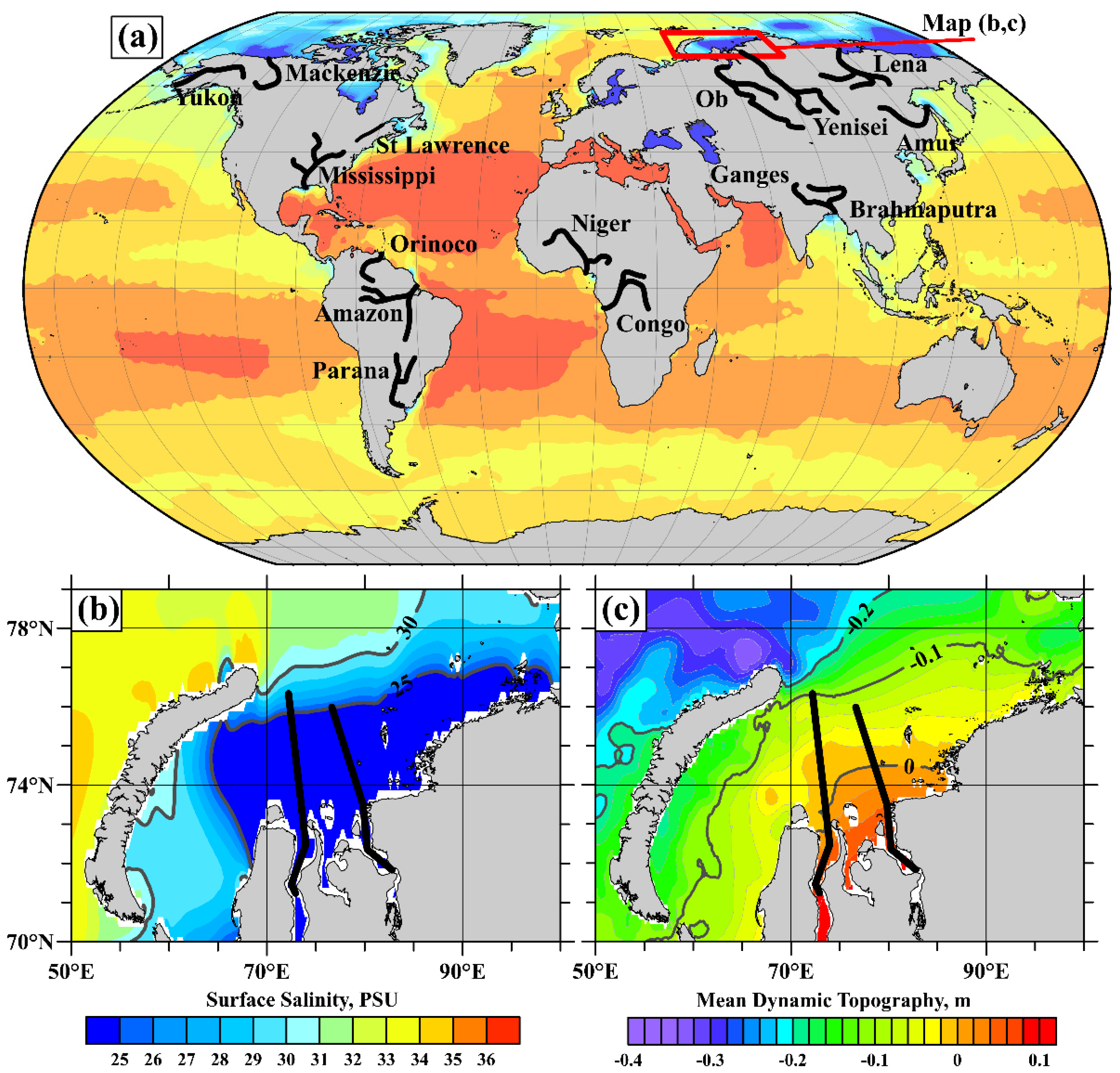
In this study, we analyze applicability of satellite altimetry for studying the Ob–Yenisei plume in the Arctic Ocean (Figure 1). The Ob–Yenisei plume is formed in the Kara Sea by discharge from the Ob, Yenisei, and several smaller rivers. Total freshwater discharge that forms the Ob–Yenisei plume during ice-free period in the Kara Sea (June–October) is estimated as ~1000 km3 [33,34]. The isohaline of 25 is typically regarded as the outer border of the Ob–Yenisei plume. Area of the Ob–Yenisei plume during ice-free periods increases from ~100,000 km2 in July to ~200,000–250,000 km2 in September–October [8]. Depth of the Ob–Yenisei plume is 10–15 m [8]. Seasonal and inter-annual variability of the Ob–Yenisei plume during ice-free period is described in detail in [8,35,36,37].
We compare in situ salinity measurements within the Ob–Yenisei plume performed during 11 oceanographic surveys during ice-free season in 2007–2019 with synchronous satellite altimetry measurements in the study area. Based on these data, we analyze the relation between positive sea level anomaly, on the one hand, and surface and vertical salinity structure, on the other hand. Then, we analyze applicability of validated and non-validated satellite altimetry data collected during the last 28 years in the study region for detection of the Ob–Yenisei plume and describe its seasonal and interannual variability. Finally, we provide examples when straightforward usage of satellite altimetry for detection of the Ob–Yenisei plume could lead to incorrect results.
This paper is organized as follows. In Section 2, we provide information about in situ and satellite altimetry data used in this study. Section 3 is focused on the comparison of satellite sea level anomaly data and in situ salinity measurements in the study area. Applicability of satellite altimetry data for studying the Ob–Yenisei plume is discussed in Section 4, followed by the conclusions.
2. Data and Methods
2.1. Data Used
The hydrographic in situ data used in this study were collected during 11 oceanographic surveys in the Kara Sea onboard the research vessels “Akademik Mstislav Keldysh” and “Professor Shtokman” in 2007, 2011, and 2013–2019. The field surveys included continuous measurements of salinity in the sea surface layer (2–3-m depth) performed along the ship track using a shipboard pump-through system equipped with a thermosalinograph (SBE 21 SeaCAT). In 2007, 2011, 2014, and 2016 the vertical thermohaline structure was measured at multiple hydrographic stations in the central part of the Kara Sea including the spreading area of the Ob–Yenisei plume. Vertical thermohaline structure was measured using a CTD instrument (SBE 911plus) at 0.2 m spatial resolution. This CTD profiler was equipped with two parallel temperature and conductivity sensors; the mean temperature differences between them did not exceed 0.01 °C, while that of salinity was not greater than 0.01 PSU. The detailed information about these measurements, as well as their comprehensive analysis are given in [8].
The Data Unification and Altimeter Combination System (DUACS) delayed time altimeter gridded product [40] available from Copernicus Marine Environment Monitoring Service (CMEMS, http://marine.copernicus.eu/, accessed date: 7 December 2021) was analyzed in this study. This product comprises maps of sea level anomaly (SLA), absolute dynamic topography (ADT), surface-geostrophic velocities, and surface-geostrophic velocity anomalies with a spatial resolution of 0.25° on a Mercator regular grid and a daily sampling. The data include measurements from all available altimeters at any given time. Wind forcing conditions were examined using ERA5 atmospheric reanalysis with a 0.25° spatial and hourly temporal resolution [41].
2.2. Methods
In this study, we compare the spatial extents of the Ob–Yenisei plume derived from in situ salinity and satellite altimetry data, which requires determination of the plume–sea boundary. Salinity is the main characteristic used to distinguish river plumes and seawater. In the previous related studies, the boundary zones between a river plume and ambient sea were associated with a specific isohaline, which value depends on the local conditions. In the case of a sharp gradient and close location of isohalines at the plume-sea interface, the choice of a salinity value for determining the plume boundary is rather arbitrary, albeit it does not significantly affect the resulting spatial extents and area of the plume. Previous research revealed that the Ob–Yenisei plume is bounded by a distinct salinity gradient at the isohalines of 24–26 [8]. According to this result, in the current study, we prescribe the outer border of the Ob–Yenisei plume by the isohaline of 25.
Similar to salinity data, previous studies of river plumes based on various satellite data (thermal, optical, salinity, altimetry, SAR) associated sharp gradients and/or the related isolines with outer borders of river plumes [6,42,43,44,45,46,47,48,49,50]. However, direct comparison of in situ salinity measurements with satellite data used in these studies played a crucial role in assessment of validity and accuracy of satellite-derived plume borders. This comparison was based on synchronization of position and time of in situ measurements and satellite observations and the subsequent reprojection of both datasets to the same coordinate-time system.
According to previous studies, the comparison of the gridded altimetry data with in situ salinity measurements was performed in the following way. First, a point with the salinity data measured by SBE 21 SeaCAT thermosalinograph (Sea-Bird Electronics, Bellevue, WA, USA) was selected. The coordinates and exact time of salinity measurements are known from the ship GPS with high accuracy. Then, we selected the respective ADT field from daily gridded altimetry on the day of salinity measurements. This field was interpolated to the point of salinity measurements using the linear interpolation method. This procedure was performed for all points along the ship track.
3. Results
3.1. Surface Salinity Structure and ADT
River plumes are determined as water masses with reduced salinities as compared to surrounding seawater. Generally, water within river plumes differs from seawater by many other physical, optical, geochemical, and biologic properties. However, the principal difference between river plumes and surrounding sea consists in the reduced density of river plumes, which is caused by the reduced salinity of river plumes. Temperature difference also affects plume–sea density gradient, albeit it plays a secondary role. Indeed, according to the equation of state for seawater [51], the density change caused by an increase in salinity by one unit is ~10 kg/m3. The same density change caused by an increase in temperature is provided by a value ~10 °C. The typical plume–sea density differences exceed several salinity units, while the related temperature differences are much less. In particular, it is the case of the Ob–Yenisei plume (Figure 2). Seasonal variations of temperature in the Kara Sea (including the Ob–Yenisei plume) are among the largest in the World Ocean (10–15 °C); however, the salinity jump at the plume–sea border is 5–10. The prevailing role of salinity in density regulation in the study area results in almost vertical lines of density contours in the temperature–salinity diagram (Figure 2).
The reduced density (salinity) determines fundamental features of dynamics of river plumes, namely, advection in the surface layer and formation of large horizontal pressure gradient between river plume and surrounding seawater. As a result, surface salinity measurements are the only direct and reliable way to detect river plumes and determine the area they occupy at sea. Once we have intention to apply satellite altimetry to detect the Ob–Yenisei plume, we compare these data with the extensive data set of surface salinity measurements performed in the Kara Sea along the ship tracks during 11 oceanographic cruises in 2007–2019. Figure 3 demonstrates in situ surface salinity versus synchronous satellite-derived ADT.
Surface salinity and ADT have certain negative correlation, namely, ADT at low salinities (0–20) is equal to 0–25 cm, which is greater than ADT at high salinities (20–35) equal to −20–20 cm. However, the observed variability of ADT within individual salinity values is very large. In particular, ADT at salinity of 25 varies between −15 and 20 cm, while ADT at salinity of 15 varies between −5 and 25 cm. Moreover, this large variability is observed for the whole range of salinity values from 0 to 32. As a result, the common ADT range (−5–20 cm) for the Ob–Yenisei plume (salinities of 0–25) and for the ambient saline sea (salinities of 25–32) is comparable with the whole range of ADT in the Kara Sea.
Figure 3 clearly demonstrates that the ADT–salinity graph is dramatically different for different cruises at different years. Therefore, there is no universal and direct relation between surface salinity and ADT in the Kara Sea. In particular, straightforward usage of satellite altimetry for detection of the Ob–Yenisei plume is misleading. This negative result is the main outcome of this study. However, further we analyze the causes of this feature and describe conditions, when ADT is indicative of satellite salinity and could be used for detection of the Ob–Yenisei plume.
3.2. Vertical Salinity Structure and ADT
Positive sea level anomaly within the river plume depends on salinity anomaly of the plume and the plume depth. Previous research revealed significant seasonal variability of both characteristics of the Ob–Yenisei plume during ice-free season [8,35]. In June–July, during the peak river discharge, the Ob–Yenisei plume is low-saline (5–15) and relatively shallow (10 m). Then, in August–October salinity of the plume steadily increases to 15–25, its depth also increases to 10–15 m. Total freshwater volume contained in the Ob–Yenisei plume accumulates during the ice-free season from ~600 km3 in June–July to ~900 km3 in October.
These seasonal changes in structure of the Ob–Yenisei plume affect sea level anomaly of the plume and modify the related ADT–salinity relation. Indeed, decomposition of all points at the ADT–salinity graph by months shows that the sea level within the plume in October is 5–20 cm higher for the same salinities than in July (Figure 3). In July, the Ob–Yenisei plume is a spatially homogenous and strongly stratified river plume formed by flooding river runoff recently discharged to the sea. Later in August–October, river runoff significantly decreases, while the Ob–Yenisei plume experience intense mixing with subjacent saline sea [8]. As a result, the ADT–salinity relation is almost linear in July, while in August, September, and October the linear dependence disperses (Figure 3).
In order to assess the influence of variations of salinity and depth of the plume on the sea level anomaly, we calculate the freshwater content in the water column, i.e., the amount of zero-saline river water that provided the observed vertical salinity distribution once mixed with the reference saline seawater. The freshwater content L is calculated by the equation , where x and z are the horizontal and vertical coordinates, respectively, S(x,z) is the observed salinity at the point (x,z), S0 is the reference ambient seawater salinity (equal to 32 in case of the Kara Sea), h(x) is the ocean depth at the point x [8].
The freshwater content L represents the equivalent thickness of the layer of fresh waters contained in the total water column. This characteristic has potential to be more correlated with the sea level anomaly, as compared to sea surface salinity. Indeed, once a plume experiences mixing with subjacent sea, the salinity and depth of the plume increases, however, both freshwater content and ADT do not change. In order to check this assumption, we calculated the freshwater content within the Ob–Yenisei plume. Note that calculation of the freshwater content requires information about vertical salinity structure. Therefore, freshwater content could be calculated accurately only in case of vertical salinity measurements at closely spaced hydrologic stations along the transects. These appropriate measurements in the study area were performed in 2007, 2011, 2014, and 2016. The measurements were performed along two quasi-meridional transects, which started at the Ob and Yenisei estuaries, crossed the Ob–Yenisei plume, and finished in the saline sea northward from the plume (Figure 1). Both transects were repeated in July, August, and September, albeit during different years.
The freshwater content calculated along the transects shows very good accordance with ADT from the daily gridded altimetry interpolated to the points of the transects (Figure 4). The freshwater content decreases from 14–18 m in the Ob and Yenisei gulfs to zero in the ambient seawater of the Kara Sea (red lines in Figure 4). The sea level shows quite similar structure; the corresponding decrease of the sea level from the Ob and Yenisei gulfs and the ambient sea based on the altimetry data is 20–25 cm. Typical values of ADT are 10–25 cm within the plume and −10 to 0 cm in the ambient sea at the distance ~500 km northward from the gulfs, which corresponds to the mean sea level gradient of 0.04–0.05 cm/km. Note that ADT reveals only this large-scale decrease of the sea level between the plume and the northern part of the Kara Sea. Local sea level variations at smaller spatial scales do not correlate with local variations of the freshwater content making it impossible to study the internal structure of the plume based on the satellite altimetry data.
3.3. Wind Forcing and ADT
Despite seasonal changes in the plume structure, strong wind forcing also could substantially affect sea level and break the ADT–salinity correlation on a synoptic time scale. Strong and durable winds induce wind surges at the coastal areas, which is the case of the Kara Sea [32,52,53,54]. The threshold value of wind speed, which causes change of sea level by more than 10 cm in the study area (i.e., comparable with plume–sea ADT difference) is equal to 6–8 m/s [32,55]. As a result, the Ob–Yenisei plume could be correctly detected by satellite altimetry only in case of low wind forcing (<6 m/s), which occurs on average during 40% of all days during the ice-free season (July–October) based on the ERA5 reanalysis.
The ADT maps presented in Figure 5 illustrate that the increased sea level in the central part of the Kara Sea associated with the Ob–Yenisei plume could be significantly distorted during 1–2 weeks. The mean wind during the first half of September 2018 varied between 7 and 10 m/s, which is noticeably higher than the mean wind forcing in the Kara Sea. The maps are given with a time step of 3 days between 5 September and 14 September 2018. The area of elevated sea surface limited by isoline of 10 cm decreases from 205,000 km2 to 85,000 km2 during these 10 days, which is caused by the wind surge and cannot be associated with the actual decrease of the plume area. The shape of the 0 m ADT isoline is also very indicative. Its location in the central part of the Kara Sea shifts 230 km onshore during 3 days between 11 and 14 September, which is another manifestation of the wind surge.
Based on the ERA5 reanalysis, the wind between 5 and 11 September was directed to the east and southeast, leading to the wind surge in the central part of the plume (Figure 5). Note that the general direction of the shoreline changes within the plume from zonal in the central part of the Kara Sea to almost meridional at some parts of the eastern plume boundary. In addition, the plume borders Novaya Zemlya in September and October. Therefore, a strong wind of almost any direction will cause a surge for some large area of the plume.
3.4. Detection of the Ob–Yenisei Plume in July 2016
In the previous section, we demonstrated that satellite altimetry data could be used for detection of the Ob–Yenisei plume, however only under two conditions: First, ADT must be validated against recent (<1 month difference) surface salinity measurements performed across the plume–sea border. At greater temporal scale, the initial validated ADT–salinity relation changes due to seasonal variability of freshwater content within the plume. Second, wind forcing must be low (<6 m/s) during the considered period, as well as during the period of in situ measurements used for ADT validation. Strong winds induce wind surges that modify the initially validated ADT–salinity relation.
Among all other cruises, the cruise in July 2016 shows the best correlation between ADT and surface salinity (blue dots in Figure 3 and Figure 6b). Surface salinity measurements on 17–25 July 2016 are supported by vertical salinity measurements along both Ob and Yenisei transects (Figure 6a). The calculated distribution of freshwater content along these transects also shows good correlation with ADT (Figure 4). The observed good applicability of ADT data for detection of the Ob–Yenisei plume in July 2016 is supported by both conditions described above. Wind forcing in the central part of the Kara Sea was low (5 m/s on average) from the beginning of July until the period of field measurements. Later in the end of July, the average wind speed increased to 7–10 m/s. As a result, we presume that the obtained ADT–salinity relation could be applied to reconstruct the spreading area of the Ob–Yenisei plume during 1–25 July 2016 using satellite altimetry data.
The linear dependence between surface salinity and ADT during the field survey provides the value of ADT (−6 cm), which corresponds to the outer boundary of the Ob–Yenisei plume defined by isohaline of 25 (Figure 6b) [8]. Using this ADT value, we defined the outer plume boundary with a time step of 5 days during 1–25 July 2016 (Figure 7) based on daily gridded altimetry data. We obtained that the area of the Ob–Yenisei plume during this period increased from 175,000 to 248,000 km2. The mean velocity of the northward motion of the outer plume boundary was 6.5 km/day or 7.5 cm/s. This example demonstrates that satellite altimetry could provide important results about spatial extents and spreading dynamics of the Ob–Yenisei plume, albeit only after validation against appropriate in situ salinity measurements and in case of low wind forcing.
3.5. Detection of the Ob–Yenisei Plume in 2007–2019
We test the ability of satellite altimetry to detect the Ob–Yenisei plume using surface salinity measurements in the study area obtained during 11 oceanographic surveys in the Kara Sea in 2007, 2011, and 2013–2019. Based on in situ data, we reconstruct location of the outer border of the Ob–Yenisei plume at the segments where it was crossed by the ship track, i.e., areas where surface salinity was equal to 25. Then, we obtain the ADT values at the respective areas and determine the related isolines at the ADT maps of the Kara Sea, i.e., reconstruct the outer border of the Ob–Yenisei plume using satellite altimetry data. Then, in every case we test two questions: first, are the ADT values similar at different segments of the actual plume border (detected by salinity measurements) and, second, do the ADT isohalines represent realistic plume border.
Among the 16 survey periods, only six were performed under low wind forcing conditions. In cases of strong wind forcing, the ADT–salinity relation is distorted, as a result, the ADT values are different at different segments of salinity-derived plume border, and the altimetry-derived plume borders are non-realistic. Typical examples of this situation are shown in Figure 8a,b,d. For example, on 16 September 2011 (Figure 8a) the shapes of the outer plume boundary defined based on in situ salinity and satellite altimetry significantly differ. The discrepancies between the ADT isoline of −6 cm and surface salinity of 15 PSU exceed 200 km. Similar discrepancies are observed on 21 August 2014 and 23 September 2011. The mean wind in the central part of the Kara Sea in these three cases (Figure 8a,c,d) was equal 6.3, 5.2, 6.8 m/s, correspondingly. On the opposite, in rare cases of low wind forcing conditions, the ADT–salinity relation works well, and the resulting altimetry-derived plume borders generally are trustworthy (Figure 8c). Here, the mean wind is 4.5 m/s and the location of the ADT isolines corresponds to the actual plume outer boundary defined by continuous measurements of surface salinity.
As it was described above, the internal structure of the Ob–Yenisei plume is not represented correctly by ADT even if the ADT–salinity relation is correct for detection of the outer plume border. Local sea level anomalies up to 30 cm are observed in the Gulf of Ob, in the Yenisei Gulf, at shallow areas along Taymyr Peninsula, etc. (Figure 6a and Figure 8). These peculiarities of sea level are caused by low accuracy of satellite altimetry data near the shoreline and low accuracy of reconstruction of tidal component, which is subtracted from the ADT data. These features are especially evident in the narrow gulfs and over shoals, and do not represent the internal plume structure once they are compared with synchronous salinity measurements (Figure 6a).
Comparison of in situ salinity measurements performed during different months of the same year with the respective ADT maps illustrates seasonal shift of freshwater content in the Ob–Yenisei plume (Figure 9). The salinity-detected outer border of the plume in August 2018 corresponded to the ADT isolines of 0–10 cm (Figure 9a), while two months later in October 2018 it shifted to the ADT isolines of 15–20 cm (Figure 9b). The same effect is clearly seen on the July, August, September, and October mean ADT maps (Figure 10). For these maps, we averaged monthly mean ADT data available from CMEMS in a range of 2007–2019, which corresponds to the interval of our in situ measurements. Based on these data, the sea level rises from July to October. For example, at the northern end of the Gulf of Ob at a latitude of 72°45′N, the mean ADT equals to 4.6 cm (July), 6.6 cm (August), 15.1 cm (September), and 16.2 cm (October). The same values in the central part of the Kara Sea at 74°N are 4.3, 5.0, 8.5, and 12.7 cm. Thus, the mean increase of the sea level during the ice-free period is approximately 10 cm and depends on the location relative to the Ob and Yenisei Gulfs. This sea level change must be taken into account for proper detection of the outer plume border by means of satellite altimetry.
4. Discussion and Conclusions
In this study, we analyze satellite altimetry data and in situ salinity measurements in the Kara Sea to answer the question if satellite altimetry data could be used for detection of the large Ob–Yenisei plume. The extensive set of in situ salinity measurements performed during 11 oceanographic cruises in 2007–2019 in the Kara Sea clearly demonstrates the absence of universal dependence between sea level anomaly and surface salinity. On the opposite, the ADT–salinity relation is prone to very large synoptic variability caused by strong wind forcing and wind surges in the study area. Second, seasonal variability of ADT-salinity relation is caused by constant increase of ADT within the Ob–Yenisei plume from July to October due to steady accumulation of freshwater in the plume during the ice-free season.
The results clearly demonstrate that satellite altimetry could provide correct information about spatial extents and spreading dynamics of the Ob–Yenisei plume, albeit only after validation against appropriate and recently made in situ salinity measurements and in case of low wind forcing. Once ADT is validated against in situ salinity data collected more than several weeks before or after the considered period and/or covering a narrow range of salinities, the ADT-salinity relation would be incorrect. Furthermore, the ADT–salinity relation is incorrect in case of strong winds, i.e., on average during 40% of days during ice-free season in the Kara Sea. In particular, the altimetry-derived outer border of the Ob–Yenisei plume was correct during only 6 out of 16 field surveys analyzed in this study. Another important limitation of satellite altimetry data in context of this study consists in the fact that ADT does not represent internal structure of the Ob–Yenisei plume. Low accuracy of satellite altimetry data near the shoreline, as well as low accuracy of reconstruction of tidal component in the coastal area results in formation of multiple areas of local increased or decreased sea level, which are not related to internal structure of the plume. These features are especially prominent in the gulfs and over shoals.
Significant inaccuracies can be produced during spatial interpolation of altimetry data to the gridded fields, which will diminish small-scale frontal structures. However, as satellite altimetry does not reproduce even the large-scale plume structure, the along-track products will not show the small-scale features of the plume. In addition, most works dedicated to studies of the plume structure based on the altimetry use exactly gridded fields. Note that the number of available altimetry missions differs within a 2007–2019 period, which makes the altimetry data more unreliable.
We strongly support the idea that indirect methods based on remote sensing hold promise of partly substituting in situ oceanographic measurements. However, these indirect methods must be properly validated and adapted to specific regions in the World Ocean. This study provides a good example of this concept. Reconstruction of the outer border of the Ob–Yenisei plume on a daily or weekly basis during ice-free season holds promise to provide new insights about its spreading dynamics and variability on synoptic, seasonal, and interannual time scales. High-resolution satellite altimetry of the study area is available on a daily basis during the last 28 years and this dataset was considered as a possible tool for monitoring the Ob–Yenisei plume. However, our results clearly demonstrate that satellite altimetry should be limitedly applied for detection of the Ob–Yenisei plume due to lack of regular in situ salinity measurements and rare low wind forcing conditions in the study area. Therefore, straightforward usage of positive anomaly of satellite altimetry as a proxy of the Ob–Yenisei plume is prone to large uncertainties and could produce misleading results.
Limited applicability of satellite altimetry for detection of the Ob–Yenisei plume described in this study could be relevant for other large river plumes in the World Ocean. Due to limitations of spatial resolution and accuracy of satellite altimetry, the obtained results are relevant only to the Amazon–Orinoco, Ganges–Brahmaputra, Congo, and Lena plumes. However, these river plumes affect a number of key physical, biological and geochemical processes (water balance, stratification, nutrient cycle, carbon cycle, acidification, etc.) across large marine areas including the Bay of Bengal [28,56,57], the South China Sea [58], the central Atlantic [59,60], and the Arctic Ocean [8,9,35,36,37,61,62,63]. Moreover, spreading and mixing of Ob–Yenisei and Lena plumes in the Arctic Ocean determine the sea stratification in the area of seasonal sea ice formation, thereby affecting ice formation in the Arctic Ocean, seasonal variability in the Earth’s albedo and planetary climate [64,65].
In conclusion, the important motivation of this work is to highlight to the community of ocean scientists that straightforward usage of satellite data without proper validation can be (and very often is) misleading. River plumes are distinctly visible at wide variety of satellite products due to their significantly different physical, optical, geochemical, and biologic properties as compared to surrounding sea. Moreover, many of these satellite products have regular planetary coverage and open data access. On the other hand, in situ measurements within river plumes are often limited or not available because field surveys are laborious and expensive. Therefore, river plumes (and other prominent features at the ocean surface) are often studied using solely or almost solely satellite data, which has high risk of incorrect results. This work clearly demonstrates that high correlation between satellite-derived parameters and salinity neither provides correct detection of river plume borders, nor trustworthy information about its internal structure. The comparison of satellite-derived parameters and salinity should be done point-to-point with particular attention paid to correct representation of intermediate salinity values.
This is not only the case of satellite altimetry. In particular, the recent study by Tarasenko et al. [32] used satellite-derived salinity to describe structure and variability of the large Lena plume in the Arctic Ocean. However, satellite salinity was not properly validated against in situ data for intermediate and low-saline shelf areas (i.e., to the Lena plume itself), validation in fact was limited to calculation of correlation of two datasets. As a result, the presented satellite-derived salinity distributions did not reproduce sharp salinity gradients typical for the outer border of the Lena plume. The area of the Lena plume was overestimated due to artifacts of satellite-derived salinity, which became the basis for highly speculative discussion by Tarasenko et al. [32] about temporal variability of the Lena plume.
Author Contributions
Conceptualization, D.F. and A.O.; formal analysis, D.F. and A.O.; writing, D.F. and A.O. All authors have read and agreed to the published version of the manuscript.
Funding
This research was funded by the Ministry of Science and Higher Education of the Russian Federation, theme 0128-2021-0002 (processing of in situ data) and the Russian Science Foundation, research project 21-17-00278 (processing of satellite data).
Data Availability Statement
The in situ data are available at https://0-doi-org.brum.beds.ac.uk/10.1029/2020JC016486, accessed date: 7 December 2021. The satellite altimetry data are available at Copernicus MarineF Environment Monitoring Service (CMEMS; http://marine.copernicus.eu/, accessed date: 7 December 2021).
Conflicts of Interest
The authors declare no conflict of interest.
References
- Ostrander, C.E.; McManus, M.A.; DeCarlo, E.H.; Mackenzie, F.T. Temporal and spatial variability of freshwater plumes in a semi-enclosed estuarine–bay system. Estuaries Coasts 2008, 31, 192–203. [Google Scholar] [CrossRef]
- Korotenko, K.A.; Osadchiev, A.A.; Zavialov, P.O.; Kao, R.-C.; Ding, C.-F. Effects of bottom topography on dynamics of river discharges in tidal regions: Case study of twin plumes in Taiwan Strait. Ocean Sci. 2014, 10, 865–879. [Google Scholar] [CrossRef] [Green Version]
- Osadchiev, A.A.; Korotenko, K.A.; Zavialov, P.O.; Chiang, W.-S.; Liu, C.-C. Transport and bottom accumulation of fine river sediments under typhoon conditions and associated submarine landslides: Case study of the Peinan River, Taiwan. Nat. Haz. Earth Syst. Sci. 2016, 16, 41–54. [Google Scholar] [CrossRef]
- Osadchiev, A.A.; Sedakov, R.O.; Barymova, A.A. Response of a small river plume on wind forcing. Front. Mar. Sci. 2021, 8, 809566. [Google Scholar] [CrossRef]
- Osadchiev, A.A.; Sedakov, R.O.; Barymova, A.A.; Gordey, A.S. Internal waves as a source of concentric rings within small river plumes. Remote Sens. 2021, 13, 4275. [Google Scholar] [CrossRef]
- Grodsky, S.A.; Reverdin, G.; Carton, J.A.; Coles, V.J. Year-to-year salinity changes in the Amazon plume: Contrasting 2011 and 2012 Aquarius/SACD and SMOS satellite data. Remote Sens. Environ. 2014, 140, 14–22. [Google Scholar] [CrossRef]
- Osadchiev, A.A. Spreading of the Amur River plume in the Amur Liman, the Sakhalin Gulf, and the Strait of Tartary. Oceanology 2017, 57, 376–382. [Google Scholar] [CrossRef]
- Osadchiev, A.A.; Frey, D.I.; Shchuka, S.A.; Tilinina, N.D.; Morozov, E.G.; Zavialov, P.O. Structure of the freshened surface layer in the Kara Sea during ice-free periods. J. Geophys. Res. 2021, 126, e2020JC016486. [Google Scholar] [CrossRef]
- Osadchiev, A.A.; Frey, D.I.; Spivak, E.A.; Shchuka, S.A.; Tilinina, N.D.; Semiletov, I.P. Structure and inter-annual variability of the freshened surface layer in the Laptev and East-Siberian seas during ice-free periods. Front. Mar. Sci. 2021. [Google Scholar] [CrossRef]
- Kang, Y.; Pan, D.; Bai, Y.; He, X.; Chen, X.; Chen, C.T.A.; Wang, D. Areas of the global major river plumes. Acta Oceanol. Sin. 2013, 32, 79–88. [Google Scholar] [CrossRef]
- Boyer, E.W.; Howarth, R.W.; Galloway, J.N.; Dentener, F.J.; Green, P.A.; Vörösmarty, C.J. Riverine nitrogen export from the continents to the coasts. Glob. Biogeochem. Cycles 2006, 20, GB1S9. [Google Scholar] [CrossRef] [Green Version]
- Korshenko, E.A.; Zhurbas, V.M.; Osadchiev, A.A.; Belyakova, P.A. Fate of river-borne floating litter during the flooding event in the northeastern part of the Black Sea in October 2018. Mar. Poll. Bull. 2020, 160, 111678. [Google Scholar] [CrossRef]
- Yakushev, E.; Gebruk, A.; Osadchiev, A.; Pakhomova, S.; Lusher, A.; Berezina, A.; van Bavel, B.; Vorozheikina, E.; Chernykh, D.; Kolbasova, G.; et al. Microplastics distribution in the Eurasian Arctic is affected by Atlantic waters and Siberian rivers. Commun Earth Environ. 2021, 2, 23. [Google Scholar] [CrossRef]
- Pogojeva, M.; Zhdanov, I.; Berezina, A.; Lapenkov, A.; Kosmach, D.; Osadchiev, A.; Hanke, G.; Semiletov, I.; Yakushev, E. Distribution of floating marine macro-litter in relation to oceanographic characteristics in the Russian Arctic Seas. Mar. Poll. Bull. 2021, 166, 112201. [Google Scholar] [CrossRef]
- Milliman, J.D.; Farnsworth, K.L. River Discharge to the Coastal Ocean: A Global Synthesis; Cambridge University Press: Cambridge, UK, 2013; 393p. [Google Scholar]
- Schmidt, N.; Thibault, D.; Galgani, F.; Paluselli, A.; Sempéré, R. Occurrence of microplastics in surface waters of the Gulf of Lion (NW Mediterranean Sea): Special issue of MERMEX project: Recent advances in the oceanography of the Mediterranean Sea. Prog. Oceanogr. 2018, 163, 214–220. [Google Scholar] [CrossRef] [Green Version]
- Wiseman, W.J.; Kelly, F.J. Salinity variability within the Louisiana coastal current during the 1982 flood season. Estuaries 1994, 17, 732–739. [Google Scholar] [CrossRef]
- Tang, D.; Kester, D.R.; Ni, I.H.; Qi, Y.; Kawamura, H. In situ and satellite observations of a harmful algal bloom and water condition at the Pearl River estuary in late autumn 1998. Harmful Algae 2003, 2, 89–99. [Google Scholar] [CrossRef]
- Emmett, R.L.; Krutzikowsky, G.K.; Bentley, P. Abundance and distribution of pelagic piscivorous fishes in the Columbia River plume during spring/early summer 1998–2003: Relationship to oceanographic conditions, forage fishes, and juvenile salmonids. Prog. Oceanogr. 2006, 68, 1–26. [Google Scholar] [CrossRef]
- Born, G.H.; Tapley, B.D.; Ries, J.C.; Stewart, R.H. Accurate measurement of mean sea level changes by altimetric satellites. J. Geophys. Res. 1986, 91, 11775–11782. [Google Scholar] [CrossRef]
- Fu, L.-L.; Christensen, E.J.; Yamarone, C.A.; Lefebvre, M.; Menard, Y.; Dorrer, M.; Escudier, P. Topex/Poseidon mission overview. J. Geophys. Res. 1994, 99, 24369–24381. [Google Scholar] [CrossRef]
- Ubelmann, C.; Dibarboure, G.; Gaultier, L.; Ponte, A.; Ardhuin, F.; Ballarotta, M.; Faugère, Y. Reconstructing ocean surface current combining altimetry and future spaceborne Doppler data. J. Geophys. Res. 2021, 126, e2020JC016560. [Google Scholar] [CrossRef]
- Mulet, S.; Rio, M.H.; Etienne, H.; Artana, C.; Cancet, M.; Dibarboure, G.; Feng, H.; Husson, R.; Picot, N.; Provost, C.; et al. The new CNES-CLS18 global mean dynamic topography. Ocean Sci. 2021, 17, 789–808. [Google Scholar] [CrossRef]
- Piecuch, C.G.; Wadehra, R. Dynamic sea level variability due to seasonal river discharge: A preliminary Global Ocean model study. J. Geophys. Res. 2020, 47, e2020GL08698. [Google Scholar] [CrossRef]
- Molleri, G.S.F.; Novo, E.M.L.; Kampel, M. Space-time variability of the Amazon River plume based on satellite ocean color. Cont. Shelf Res. 2010, 30, 342–352. [Google Scholar] [CrossRef]
- Osadchiev, A.A. A method for quantifying freshwater discharge rates from satellite observations and Lagrangian numerical modeling of river plumes. Environ. Res. Lett. 2015, 10, 085009. [Google Scholar] [CrossRef] [Green Version]
- Osadchiev, A.A.; Sedakov, R.O. Spreading dynamics of small river plumes o the northeastern coast of the Black Sea observed by Landsat 8 and Sentinel-2. Remote Sens. Environ. 2019, 221, 522–533. [Google Scholar] [CrossRef]
- Wu, L.; Wang, F.; Yuan, D.; Cui, M. Evolution of freshwater plumes and salinity fronts in the northern Bay of Bengal. J. Geophys. Res. 2007, 112, C8. [Google Scholar] [CrossRef]
- Hopkins, J.; Lucas, M.; Dufau, C.; Sutton, M.; Stum, J.; Lauret, O.; Channelliere, C. Detection and variability of the Congo River plume from satellite derived sea surface temperature, salinity, ocean colour and sea level. Rem. Sens. Environ. 2013, 139, 365–385. [Google Scholar] [CrossRef]
- Kubryakov, A.; Stanichny, S.; Zatsepin, A. River plume dynamics in the Kara Sea from altimetry-based Lagrangian model, satellite salinity and chlorophyll data. Rem. Sens. Environ. 2016, 176, 177–187. [Google Scholar] [CrossRef]
- Zhuk, V.R.; Kubryakov, A.A. Interannual variability of the Lena River plume propagation in 1993-2020 on the base of satellite salinity, temperature, and altimetry measurements. Remote Sens. 2021, 13, 4252. [Google Scholar] [CrossRef]
- Tarasenko, A.; Supply, A.; Kusse-Tiuz, N.; Ivanov, V.; Makhotin, M.; Tournadre, J.; Kolodziejczyk, N.; Reverdin, G. Properties of surface water masses in the Laptev and the East Siberian seas in summer 2018 from in situ and satellite data. Ocean Sci. 2021, 17, 221–247. [Google Scholar] [CrossRef]
- Pavlov, V.K.; Timokhov, L.A.; Baskakov, G.A.; Kulakov, M.Y.; Kurazhov, V.K.; Pavlov, P.V.; Pivovarov, S.V.; Stanovoy, V.V. Hydrometeorological Regime of the Kara, Laptev, and East-Siberian Seas; University of Washington: Washington, DC, USA, 1996. [Google Scholar]
- Gordeev, V.V.; Martin, J.M.; Sidorov, J.S.; Sidorova, M.V. A reassessment of the Eurasian river input of water, sediment, major elements, and nutrients to the Arctic Ocean. Am. J. Sci. 1996, 296, 664–691. [Google Scholar] [CrossRef]
- Osadchiev, A.A.; Izhitskiy, A.S.; Zavialov, P.O.; Kremenetskiy, V.V.; Polukhin, A.A.; Pelevin, V.V.; Toktamysova, Z.M. Structure of the buoyant plume formed by Ob and Yenisei river discharge in the southern part of the Kara Sea during summer and autumn. J. Geophys. Res. 2017, 122, 5916–5935. [Google Scholar] [CrossRef]
- Osadchiev, A.A.; Asadulin, E.E.; Miroshnikov, A.Y.; Zavialov, I.B.; Dubinina, E.O.; Belyakova, P.A. Bottom sediments reveal inter-annual variability of interaction between the Ob and Yenisei plumes in the Kara Sea. Sci. Rep. 2019, 9, 18642. [Google Scholar] [CrossRef] [PubMed]
- Osadchiev, A.A.; Pisareva, M.N.; Spivak, E.A.; Shchuka, S.A.; Semiletov, I.P. Freshwater transport between the Kara, Laptev, and East-Siberian seas. Sci. Rep. 2020, 10, 13041. [Google Scholar] [CrossRef]
- Zweng, M.M.; Reagan, J.R.; Seidov, D.; Boyer, T.P.; Locarnini, R.A.; Garcia, H.E.; Mishonov, A.V.; Baranova, O.K.; Weathers, K.; Paver, C.R.; et al. World Ocean Atlas 2018, Volume 2: Salinity; NOAA Atlas NESDIS 82; Mishonov, A., Ed.; National Centers for Environmental Information: Silver Spring, MD, USA, 2018; 50p. [Google Scholar]
- Wessel, P.; Smith, W.H. A global, self-consistent, hierarchical, high-resolution shoreline database. J. Geophys. Res. 1996, 101, 8741–8743. [Google Scholar] [CrossRef] [Green Version]
- Pujol, M.-I.; Faugère, Y.; Taburet, G.; Dupuy, S.; Pelloquin, C.; Ablain, M.; Picot, N. DUACS DT2014: The new multi-mission altimeter data set reprocessed over 20 years. Ocean Sci. 2016, 12, 1067–1090. [Google Scholar] [CrossRef] [Green Version]
- Hersbach, H.; Bell, B.; Berrisford, P.; Hirahara, S.; Horányi, A.; Muñoz-Sabater, J.; Nicolas, J.; Peubey, C.; Radu, R.; Schepers, D.; et al. The ERA5 global reanalysis. Q. J. R. Meteorol. Soc. 2020, 146, 1999–2049. [Google Scholar] [CrossRef]
- DiGiacomo, P.M.; Washburn, L.; Holt, B.; Jones, B.H. Coastal pollution hazards in southern California observed by SAR imagery: Stormwater plumes, wastewater plumes, and natural hydrocarbon seeps. Mar. Poll. Bull. 2004, 49, 1013–1024. [Google Scholar] [CrossRef] [PubMed]
- Zheng, Q.; Cmente-Colón, P.; Yan, X.H.; Liu, W.T.; Huang, N.E. Satellite synthetic aperture radar detection of Delaware Bay plumes: Jet-like feature analysis. J. Geophys. Res. Ocean. 2004, 109, C03031. [Google Scholar] [CrossRef]
- Warrick, J.A.; Mertes, L.A.K.; Washburn, L.; Siegel, D.A. Dispersal forcing of southern California river plumes, based on field and remote sensing observations. Geo.-Mar. Lett. 2004, 24, 46–52. [Google Scholar] [CrossRef]
- Nezlin, N.P.; DiGiacomo, P.M. Satellite ocean color observations of stormwater runoff plumes along the San Pedro Shelf (southern California) during 1997 to 2003. Continent. Shelf Res. 2005, 25, 1692–1711. [Google Scholar] [CrossRef]
- Nezlin, N.P.; DiGiacomo, P.M.; Diehl, D.W.; Jones, B.H.; Johnson, S.C.; Mengel, M.J.; Reifel, K.M.; Warrick, J.A.; Wang, M. Stormwater plume detection by MODIS imagery in the southern California coastal ocean. Estuar. Coast. Shelf Sci. 2008, 80, 141–152. [Google Scholar] [CrossRef]
- Lihan, T.; Saitoh, S.I.; Iida, T.; Hirawake, T.; Iida, K. Satellite-measured temporal and spatial variability of the Tokachi River plume. Estuar. Coast. Shelf Sci. 2008, 78, 237–249. [Google Scholar] [CrossRef]
- Piola, A.R.; Romero, S.I.; Zajaczkovski, U. Space–time variability of the Plata plume inferred from ocean color: Synoptic characterization of the Southeastern South American Continental shelf: The NICOP/Plata Experiment. Cont. Shelf Res. 2008, 28, 1556–1567. [Google Scholar] [CrossRef]
- Jiang, L.; Yan, X.H.; Klemas, V. Remote sensing for the identification of coastal plumes: Case studies of Delaware Bay. Int. J. Remote Sens. 2009, 30, 2033–2048. [Google Scholar] [CrossRef]
- Grodsky, S.A.; Reul, N.; Lagerloef, G.; Reverdin, G.; Carton, J.A.; Chapron, B.; Quilfen, Y.; Kudryavtsev, V.N.; Kao, H.Y. Haline hurricane wake in the Amazon/Orinoco plume: AQUARIUS/SACD and SMOS observations. Geophys. Res. Lett. 2012, 39, L20603. [Google Scholar] [CrossRef] [Green Version]
- Fofonoff, N.P.; Millard, R.C., Jr. Algorithms for the Computation of Fundamental Properties of Seawater; UNESCO: Paris, France, 1983; 58p. [Google Scholar]
- Pavlidis, Y.A.; Leontev, I.O.; Nikiforov, S.L.; Rahold, F.; Grigoriev, M.N.; Razumov, S.R.; Vasilev, A.A. General prognostic scheme of the coastal zone development in Eurasian Arctic seas in the 21st century. Oceanology 2007, 47, 129–140. [Google Scholar] [CrossRef]
- Novikova, A.; Belova, N.; Baranskaya, A.; Aleksyutina, D.; Maslakov, A.; Zelenin, E.; Shabanova, N.; Ogorodov, S. Dynamics of Permafrost Coasts of Baydaratskaya Bay (Kara Sea) Based on Multi-Temporal Remote Sensing Data. Remote Sens. 2018, 10, 1481. [Google Scholar] [CrossRef] [Green Version]
- Danielson, S.L.; Hennon, T.D.; Hedstrom, K.S.; Pnyushkov, A.V.; Polyakov, I.V.; Carmack, E.; Filchuk, K.; Janout, M.; Makhotin, M.; Williams, W.J.; et al. Oceanic routing of wind-sourced energy along the Arctic continental shelves. Front. Mar. Sci. 2020, 7, 509. [Google Scholar] [CrossRef]
- Osadchiev, A.A.; Konovalova, O.P.; Gordey, A.S. Water exchange between the Gulf of Ob and the Kara Sea during ice-free seasons: The roles of river discharge and wind forcing. Front. Mar. Sci. 2021, 126, e2020JC016486. [Google Scholar] [CrossRef]
- Pant, V.; Girishkumar, M.S.; Udaya Bhaskar, T.V.S.; Ravichandran, M.; Papa, F.; Thangaprakash, V.P. Observed interannual variability of near-surface salinity in the Bay of Bengal. J. Geophys. Res. Ocean. 2015, 120, 3315–3329. [Google Scholar] [CrossRef]
- Fournier, S.; Vialard, J.; Lengaigne, M.; Lee, T.; Gierach, M.M.; Chaitanya, A.V.S. Modulation of the Ganges-Brahmaputra River plume by the Indian Ocean dipole and eddies inferred from satellite observations. J. Geophys. Res. Ocean. 2017, 122, 9591–9604. [Google Scholar] [CrossRef] [Green Version]
- Qiu, C.; Huo, D.; Liu, C.; Cui, Y.; Su, D.; Wu, J.; Ouyang, J. Upper vertical structures and mixed layer depth in the shelf of the northern South China Sea. Cont. Shelf Res. 2019, 174, 26–34. [Google Scholar] [CrossRef]
- Nikiema, O.; Devenon, J.-L.; Baklouti, M. Numerical modeling of the Amazon River plume. Cont. Shelf Res. 2007, 27, 873–899. [Google Scholar] [CrossRef]
- Vic, C.; Berger, H.; Tréguier, A.M.; Couvelard, X. Dynamics of an equatorial river plume: Theory and numerical experiments applied to the Congo plume case. J. Phys. Oceanogr. 2013, 44, 980–994. [Google Scholar] [CrossRef] [Green Version]
- Spivak, E.A.; Osadchiev, A.A.; Semiletov, I.P. Structure and variability of the Lena river plume in the south-eastern part of the Laptev Sea. Oceanology. 2021, 61, 832–836. [Google Scholar] [CrossRef]
- Osadchiev, A.A.; Medvedev, I.P.; Shchuka, S.A.; Kulikov, M.E.; Spivak, E.A.; Pisareva, M.A.; Semiletov, I.P. Influence of estuarine tidal mixing on structure and spatial scales of large river plumes. Ocean Sci. 2020, 16, 781–798. [Google Scholar] [CrossRef]
- Osadchiev, A.A.; Silvestrova, K.P.; Myslenkov, S.A. Wind-driven coastal upwelling near large river deltas in the Laptev and East-Siberian seas. Remote Sens. 2020, 12, 844. [Google Scholar] [CrossRef] [Green Version]
- Carmack, E.C.M.; Yamamoto-Kawai, T.W.; Haine, S.; Bacon, B.A.; Bluhm, C.; Lique, H.; Melling, I.V.; Polyakov, F.; Straneo, M.L.; Williams, W.J. Freshwater and its role in the Arctic Marine System: Sources, disposition, storage, export, and physical and biogeochemical consequences in the Arctic and global oceans. J. Geophys. Res. Biogeosci. 2016, 121, 675–717. [Google Scholar] [CrossRef]
- Nummelin, A.; Ilicak, M.; Li, C.; Smedsrud, L.H. Consequences of future increased Arctic runoff on Arctic Ocean stratification, circulation, and sea ice cover. J. Geophys. Res. Ocean. 2016, 121, 617–637. [Google Scholar] [CrossRef] [Green Version]
Figure 1.
Average summer (July–September) sea surface salinity in the World Ocean (a), the same salinity data in the area of the Ob–Yenisei plume in the Kara Sea (b), and mean dynamic topography in the Kara Sea (c). Red lines in panel (a) show the limits of maps (b,c). Salinity data are presented from World Ocean Atlas 2018 (WOA2018, [38]). Mean Dynamic Topography data are according [23] data. The shoreline is shown according to the GSHHS data [39] hereafter. Salinity color scale is the same for maps (a,b). Locations of the Ob and Yenisei transects are shown in panels (b,c) by solid black lines.

Figure 2.
Temperature–salinity diagram including the freezing point temperature (magenta line) and sigma-contours (gray lines) in the surface layer of the Kara Sea based on in situ measurements in July (blue dots), August (green dots), September (yellow dots), and October (orange dots).
Figure 2.
Temperature–salinity diagram including the freezing point temperature (magenta line) and sigma-contours (gray lines) in the surface layer of the Kara Sea based on in situ measurements in July (blue dots), August (green dots), September (yellow dots), and October (orange dots).

Figure 3.
Absolute dynamic topography versus surface salinity along the ship tracks in the Kara Sea obtained in oceanographic cruises in 2007–2019. Measurements carried out in different months are shown in different colors.
Figure 3.
Absolute dynamic topography versus surface salinity along the ship tracks in the Kara Sea obtained in oceanographic cruises in 2007–2019. Measurements carried out in different months are shown in different colors.

Figure 4.
Freshwater content (solid red lines) and ADT during in situ measurements (dotted black lines) along three Ob transects performed in July 2016, August 2014, and September 2007 (left panels) and along three Yenisei transects performed in July 2016, August 2014, and September 2011 (right panels).

Figure 5.
ADT maps in the Kara Sea with a time step of 3 days between 5 September and 14 September 2018 based on daily gridded altimetry data in case of strong wind. The ADT isolines of −0.1, 0, and 0.1 m are shown by thick black lines. The wind direction and magnitude are shown in the lower right corner of each panel based on the ERA5 reanalysis.

Figure 6.
Map of Absolute Dynamic Topography (ADT) on 20 July, solid black lines denote the Ob and Yenisei transects with continuous measurements of temperature and salinity (a), and dependence between ADT and measured salinity in the surface layer (red dots) and the linear fit of these data (black line) (b).

Figure 7.
Positions of the outer boundary of the Ob–Yenisei plume determined by the ADT isoline of −6 cm on 1–20 July 2016.
Figure 7.
Positions of the outer boundary of the Ob–Yenisei plume determined by the ADT isoline of −6 cm on 1–20 July 2016.

Figure 8.
Absolute dynamic topography maps in the Kara Sea on (a) 16 September 2011, (b) 21 August 2014, (c) 22 September 2015, and (d) 23 September 2017. Outer boundaries of the plume defined as locations of the isohalines of 25 PSU (solid lines) in the Kara Sea are shown based on continuous salinity measurements along the ship tracks.

Figure 9.
Absolute dynamic topography maps in the Kara Sea on (a) 21 August 2018 and (b) 21 October 2018. Outer boundaries of the plume defined as locations of the isohalines of 25 PSU (solid lines) in the Kara Sea are shown based on continuous salinity measurements along the ship tracks.
Figure 9.
Absolute dynamic topography maps in the Kara Sea on (a) 21 August 2018 and (b) 21 October 2018. Outer boundaries of the plume defined as locations of the isohalines of 25 PSU (solid lines) in the Kara Sea are shown based on continuous salinity measurements along the ship tracks.

Figure 10.
Maps of mean absolute dynamic topography in July, August, September, and October. The monthly mean dynamic topography data available from CMEMS were averaged in a range of 2007–2019. The ADT isolines of −0.1, 0, and 0.1 are shown with thick black lines.
Figure 10.
Maps of mean absolute dynamic topography in July, August, September, and October. The monthly mean dynamic topography data available from CMEMS were averaged in a range of 2007–2019. The ADT isolines of −0.1, 0, and 0.1 are shown with thick black lines.

Publisher’s Note: MDPI stays neutral with regard to jurisdictional claims in published maps and institutional affiliations. |
© 2021 by the authors. Licensee MDPI, Basel, Switzerland. This article is an open access article distributed under the terms and conditions of the Creative Commons Attribution (CC BY) license (https://creativecommons.org/licenses/by/4.0/).
Share and Cite
MDPI and ACS Style
Frey, D.; Osadchiev, A. Large River Plumes Detection by Satellite Altimetry: Case Study of the Ob–Yenisei Plume. Remote Sens. 2021, 13, 5014. https://0-doi-org.brum.beds.ac.uk/10.3390/rs13245014
AMA Style
Frey D, Osadchiev A. Large River Plumes Detection by Satellite Altimetry: Case Study of the Ob–Yenisei Plume. Remote Sensing. 2021; 13(24):5014. https://0-doi-org.brum.beds.ac.uk/10.3390/rs13245014
Chicago/Turabian StyleFrey, Dmitry, and Alexander Osadchiev. 2021. "Large River Plumes Detection by Satellite Altimetry: Case Study of the Ob–Yenisei Plume" Remote Sensing 13, no. 24: 5014. https://0-doi-org.brum.beds.ac.uk/10.3390/rs13245014
Note that from the first issue of 2016, this journal uses article numbers instead of page numbers. See further details here.