Article

Global Vegetation Photosynthetic Phenology Products Based on MODIS Vegetation Greenness and Temperature: Modeling and Evaluation

1
State Key Laboratory of Subtropical Silviculture, Zhejiang A&F University, Hangzhou 311300, China
2
Key Laboratory of Carbon Cycling in Forest Ecosystems and Carbon Sequestration of Zhejiang Province, Zhejiang A&F University, Hangzhou 311300, China
3
School of Environmental and Resources Science, Zhejiang A&F University, Hangzhou 311300, China
*
Author to whom correspondence should be addressed.
Remote Sens. 2021, 13(24), 5080; https://0-doi-org.brum.beds.ac.uk/10.3390/rs13245080
Submission received: 6 November 2021 / Revised: 10 December 2021 / Accepted: 11 December 2021 / Published: 14 December 2021

Abstract

:
Land surface phenology (LSP) products that are derived from different data sources have different definitions and biophysical meanings. Discrepancies among these products and their linkages with carbon fluxes across plant functional types and climatic regions remain somewhat unclear. In this study, to differentiate LSP related to gross primary production (GPP) from LSP related to remote sensing data, we defined the former as vegetation photosynthetic phenology (VPP), including the starting and ending days of GPP (SOG and EOG, respectively). Specifically, we estimated VPP based on a combination of observed VPP from 145 flux-measured GPP sites together with the vegetation index and temperature data from MODIS products using multiple linear regression models. We then compared VPP estimates with MODIS LSP on a global scale. Our results show that the VPP provided better estimates of SOG and EOG than MODIS LSP, with a root mean square error (RMSE) for SOG of 12.7 days and a RMSE for EOG of 10.5 days. The RMSE was approximately three weeks for both SOG and EOG estimates of the non-forest type. Discrepancies between VPP and LSP estimates varied across plant functional types (PFTs) and climatic regions. A high correlation was observed between VPP and LSP estimates for deciduous forest. For most PFTs, using VPP estimates rather than LSP improved the estimation of GPP. This study presents a useful method for modeling global VPP, investigates in detail the discrepancies between VPP and LSP, and provides a more effective global vegetation phenology product for carbon cycle modeling than the existing ones.

1. Introduction

Land surface phenology (LSP) is defined as the seasonal pattern of variation in vegetated land surfaces [1,2]. Because photosynthetic carbon uptake is closely associated with the length of the growing season, LSP has been widely used to discover the effects of climate change on vegetation biophysical processes, especially related to carbon exchange between the atmosphere and terrestrial ecosystems [3,4]. Various data sources have been applied to extract LSP, including remote sensing, ground camera imagery, and FLUXNET measurements [4,5,6,7,8]. The phenological metrics of vegetation obtained from these different data sources have various definitions and biophysical meanings [9]. However, spatial- and species-specific discrepancies as well as the effectiveness in accurately describing variations in vegetation carbon fluxes among these vegetation phenological metrics remain unclear.
Remote sensing data have been widely used to extract LSP data and analyze their regional- to global-scale changes [3,6]. Time series of vegetation indices include three key transition dates, namely the start of the growing season (SOS), the end of the growing season (EOS), and the length of the growing season (LOS). The SOS and EOS indicate the timing of vegetated land surface green-up and dormancy, respectively [2,6].
In addition to remote sensing data, an increasing number of studies have focused on the retrieval of LSP through flux-measured gross primary productivity (GPP) [10,11,12,13]. Key transition dates derived from GPP are commonly defined as in LSP, including SOS and EOS [7,14,15]. However, results from previous studies indicate that LSP dates derived from GPP are related to the starting and ending days of photosynthetic phenology [11,16], which differ from the LSP derived from remote sensing data [11]. Unlike LSP from remote sensing data that represents the annual cycle of leaf coloration, LSP from flux-measured GPP more objectively represents the key transitions of ecosystem processes, such as vegetation carbon fluxes [11,13,14]. Therefore, to differentiate from LSP obtained using remote sensing data, we refer to LSP dates from GPP as vegetation photosynthetic phenology (VPP), based on previous studies on photosynthetic phenology [4,11,16]. Three key VPP dates, including the starting and ending days of GPP (SOG and EOG, respectively) and the length of the photosynthetic phenology season (LOG), were defined and used in this study.
The VPP is related to the LSP and is controlled by it, yet the two metrics are not identical and have different biophysical meanings. A study based on the comparison between LSP from remotely sensed vegetation indices and VPP from GPP showed that LSP estimates were not equivalent to VPP estimates and differed in both the sign and magnitude of lags [11]. Furthermore, the relationship between LSP and VPP varied across the same plant functional type (PFT), implying that LSP and VPP do not covary each other in the same direction [11]. A large difference was found between LSP and VPP estimates, particularly for evergreen needle forests (ENFs), which feature relatively stable seasonal variation in vegetation indices [17]. The main reason for these differences is that LSP and VPP are regulated by different driving factors. While LSP largely depends on the intra-annual changes in canopy greenness, VPP is strongly regulated by external factors, such as temperature, radiation, and precipitation [18,19,20]. Among these external factors, temperature is an important driver of variation for VPP in boreal and temperate regions [12]. Investigating the difference between LSP and VPP and improving our understanding of the relationship between phenology metrics and carbon fluxes are important for accurately estimating carbon fluxes based on land surface models. This can further our understanding of the effects of global change on the carbon cycle [11,21,22,23].
Due to the limited number and spatial distribution of FLUXNET sites, VPP from GPP measures cannot provide adequate information for a study at the global level. Predicting VPP by upscaling FLUXNET measurements using remote sensing data is a feasible technique to obtain VPP estimates across a range of spatial and temporal scales [7]. Previous studies have confirmed that a combination of LSP or vegetation indices and land surface temperature (LST) derived from MODIS data can be used to explain the VPP values for deciduous and evergreen needle forests at the site scale [7,24]. However, the effectiveness of this method in modeling global VPP and comparing LSP and VPP effects on GPP estimation is still limited.
In this study, FLUXNET site-level VPP observations were extracted from GPP estimates derived from FLUXNET measurements. Then, the global VPP products were estimated based on the relationship between site-level VPP observations and MODIS LST (MOD11A2) and enhanced vegetation index (EVI, MOD13Q1) products in 2001–2017 using a statistical regression method. The VPP estimates were then compared with LSP estimates from MODIS products (MCD12Q2, hereafter referred to as MODIS-LSP). Within this context, the objectives of this study are: (1) to construct a series of statistical regression models for estimating the global VPP of different PFTs and map long-term global VPP products; (2) to compare the discrepancies between VPPest and MODIS-LSP estimates across different PFTs and climatic regions; and (3) to investigate whether VPP is superior to LSP in estimating global vegetation photosynthetic carbon uptake.

2. Materials and Methods

2.1. Site Description

In this study, we used the FLUXNET2015 dataset and selected the site-year of daily GPP data with over 80% of the quality flag > 0.8. The quality flag indicates the percentage of measured and good-quality gap-filled data [25]. The FLUXNET2015 dataset has been quality-controlled and gap-filled according to strict quality standards [25,26,27]. The vegetation type of the site was classified into sixteen PFTs based on the International Geosphere–Biosphere Program (IGBP) land cover classification scheme [28]. In total, 145 flux sites covering 785 site-years of daily GPP data (GPP_DT_VUT_REF) from 2000 to 2014 were downloaded from the FLUXNET2015 dataset (https://fluxnet.fluxdata.org/) (15 May 2021), including 32 ENF (N = 215), 20 deciduous broadleaf forests (DBF, N = 132), 8 mixed forests (MF, N = 62), 2 closed shrublands (CSH, N = 10), 8 open shrublands (OSH, N = 29), 6 savannas (SAV, N = 15), 6 woody savannas (WSA, N = 34), 26 grasslands (GRA, N = 106), 20 wetlands (WET, N = 80), and 17 croplands (CRO, N = 102). These sites are shown in Figure 1, and their characteristics are listed in Table S1.

2.2. Site-Level VPP Observations from FLUXNET Measurements

Based on the method proposed in [3], site-level VPP observations were extracted from daily GPP estimates derived from FLUXNET measurements. First, long-term daily GPP estimates of all years from the given site were smoothed using the Savitzky–Golay filter based on the embedded function in the MATLAB R2013a environment. The Savitzky–Golay filter has been successfully used for reconstructing high-quality normalized difference vegetation indices (NDVIs) and leaf area index time series datasets [29]. The general equation of the filter can be found in [29]. It has been used in numerous studies to extract vegetation phenology data [16,17,30]. Two parameters for the filter should be determined, including the degree of the polynomial and smoothing window. A suitably large smoothing window can more effectively smoothen the sharp peaks (outliers) caused by steep changes in environmental factors in the time series of daily GPP. Results from previous studies indicate an optimal smoothing window width of 9 (approximately 91 days) for reconstructing a high-quality 10-day NDVI time-series data set based on the Savitzky–Golay filter for 14 kinds of vegetation types [29]. A data analysis also showed that differences in SOG and EOG observations using smoothing windows of 91 and 15 days were 3 and 5 days for DBF sites and 2 and 1 days for ENF sites, respectively. Therefore, based on data analysis and results from previous studies, in our study, the degree of the polynomial was 2 and the width of the smoothing window was 91 days [29,31].
Second, we calculated the amplitude of each year for the given site, equaling the maximum value of the smoothed daily GPP minus the minimum value. Finally, a relative threshold method was repeatedly used to extract the SOG and EOG [10]. Dates extracted using different thresholds represent different phases of the seasonal cycles of GPP [10], and a commonly used threshold equates to 10% of the growing season amplitude to represent the start and end of photosynthesis phenology from GPP [17,32]. Previous studies have shown that LSPs derived from different methods have large discrepancies [33]. In our study, consistent with the threshold used to extract the latest MODIS-LSP product by [34], we set the threshold for extracting SOG and EOG at 15% of the long-term average amplitude for the given site. Thus, the SOG and EOG values for each year for each site were extracted based on the first and last dates, respectively, when the smoothed daily GPP reached a threshold of 15% (Figure S1). The SOG using a threshold of 15% occurred 5 and 6 days later than when using a threshold of 10%, while the EOG was 7 and 9 days earlier than when using a threshold of 10% for DBF and ENF sites, respectively. The definitions of the seasons for the Southern hemisphere were reversed to be consistent with the seasons for the Northern hemisphere. For example, the spring season is defined as March–April–May in the northern hemisphere and September–October–November in the Southern hemisphere. The seasons for the EVI and LST data sets were also reversed for the Southern hemisphere.

2.3. Global VPP Estimates from MODIS EVI and Land Surface Temperature

A combined function of EVI and LST can well explain variation in GPP because of close correlations between EVI and light-use efficiency and between LST and environmental variables, such as radiation and vapor pressure deficit [35,36]. This provides a sound theoretical basis for estimating VPP using a regression model driven by EVI and LST. Multiple linear regression models for different PFTs were developed based on the relationships between site-level VPP observations and MODIS EVI and LST data [24]. The EVI data from the MODIS/Terra Vegetation Indices 16-Day L3 Global 250-m SIN Grid (MOD13Q1) [37] and the LST data from the MODIS/Terra LST/Emissivity 8-day L3 Global 1-km SIN Grid V006 (MOD11A2) [38] were used during the process of model construction. For each site, the EVI and LST data were extracted from a single MODIS pixel covering the FLUXNET site. Low quality values for both EVI and LST data were removed based on quality assurance (QA) layers, such as pixel reliability values from the MOD13Q1 dataset for the EVI data and mandatory QA flags from the MOD11A2 dataset for the LST data. The EVI data were masked when their corresponding pixel reliability was equal to 2 or 3, and the LST data were removed when their corresponding mandatory QA flags were equal to “10”. If the percentage of poor values was > 30%, or if a long period of poor values was observed over two sequential time steps (32 days for EVI data and 16 days for LST data) during DOY 65 to 334 (i.e., the period of active plant growth), the site-year of the data was not used. Following this process, both 16-day EVI and 8-day LST values were linearly interpolated into daily values. Then, the same was done with the daily GPP estimates, and both site-level daily EVI and LST values were smoothed using the Savitzky–Golay filter.
A previous study has reported on the strong explanatory ability of the mean and standard deviation of seasonal EVI and LST for SOS and EOS modeling [24]. In addition, we hypothesize that inter-annual variations in SOG and EOG are strongly related to EVI and LST values at five key time points during the year that shape the curves of daily EVI and LST. Therefore, twenty-eight original independent variables were obtained from smoothed daily EVI and LST data for modeling site-level VPP estimates (Table S2). These include the mean, standard deviation, and coefficient of variation of seasonal EVI and LST [24,31]. The EVI and LST values at five key time points, including the start of each season (spring, DOY 60; summer, DOY 152; autumn, DOY 243; winter, DOY 334 for the Northern hemisphere and spring, DOY 243; summer, DOY 334; autumn, DOY 60; winter, DOY 152 for the Southern hemisphere) and the maximum value during summer, were used in this study, as they shape the curves of daily EVI and LST [31]. A detailed description of these independent variables is shown in Table S2. We used a stepwise selection method to select the independent variables from the 28 original independent variables using significance levels of 0.05 and 0.1 (default values in SPSS software) as thresholds for adding and removing independent variables, respectively. Thus, we developed PFT-specific multiple linear regression models for estimating the SOG (Appendix A) and EOG (Appendix B) of each PFT.
The PFT-specific multiple linear regression models were then applied to estimate global VPP. The 16-day EVI from the MOD13C1 v006 product and the 8-day LST from the MOD11C2 v006 product at a 0.05° spatial resolution were used for global-scale VPP estimation. The independent variables were extracted from the smoothed EVI and LST time series. The global PFT map is from the MCD12C1 v006 product based on the IGBP classification schemes. Finally, the independent variables were added to the multiple linear regression models to produce a distribution map of global SOG and EOG estimates for 2001–2017.
Notably, the majority of EVI pixels in high latitudes (>60°N) lacked quality due to snow cover [39], resulting in large uncertainties in SOG and EOG estimates. A growing number of studies show that vegetation phenology in high-latitude regions is closely related to ice/snow cover [2,40,41,42,43,44,45,46]. We assume that photosynthetic carbon uptake is zero if the vegetation is covered by ice/snow and the land surface temperature is below 278 K [45]. According to observations by [44], the SOS date occurred later than the last (snowmelt) date of lingering snowpack (LDS), and the EOS date occurred before the first (snowfall) date of lingering snowpack (FDS). Furthermore, a significant relationship was observed between snow timing and vegetation phenology metrics in high-latitude regions [44]. Based on the above analysis, we used the following strategy to correct SOG and EOG estimates for pixels covered by ice/snow in high-latitude regions. When the SOG estimate from the multiple linear regression model occurred earlier than the LDS, or the EOG estimate occurred later than the FDS together with a land surface temperature below 278 K, these estimates were defined as unreasonable. These unreasonable SOG and EOG estimates were then respectively replaced with the corresponding estimates from the relationships between SOG observations and LDS, and between EOS observations and FDS (Figure 2), derived from the FLUXNET dataset. The LDS and FDS were extracted from the pixel reliability layer of the MOD13C1 v006 product. The LDS is equal to the last date when the pixel reliability is equal to 2 (indicating snow/ice coverage) during a long and consecutive ice/snow cover period between DOY 1 and 182, and the BDS is equal to the first date when the pixel reliability is equal to 2 during a long and consecutive ice/snow cover period between DOY 183 and 365 [44]. The percent of pixels for SOG and EOG estimates based on the dates of lingering snowpack was small, only accounting for 5.0% and 7.4% of the total pixels of the terrestrial area, respectively.
Additionally, the QA values for VPP estimates were constructed according to the following criteria. When the percentage of poor EVI or LST data of a pixel was less than 20% during DOY 65 to DOY 334, the reliability of the VPP estimate of the pixel was defined as high quality, and the corresponding QA value was equal to zero. When the percentage of poor EVI or LST data of a pixel was between 20% and 40% during DOY 65 to DOY 334, the reliability of the VPP estimate of the pixel was defined as medium quality, and the corresponding QA value was equal to one. When the percentage of poor EVI or LST data of a pixel was over 40% during DOY 65 to DOY 334, the reliability of the VPP estimate of the pixel was defined as low quality, and the corresponding QA value was equal to two. When the VPP values were estimated based on the LDS and FDS, the reliability of the VPP estimate of the pixel was defined as low quality, and the corresponding QA values were equal to three (Figure S2).

2.4. Evaluating Differences between VPP Estimates and MODIS-LSP Products

In order to evaluate differences between VPPest and LSP products, the most commonly used LSP products (MODIS-LSP) were compared with VPPest products. In addition, two global GPP data sets were used to analyze whether the VPPest products have closer relationships to GPP than the LSP products.

2.4.1. Comparison with MODIS-Derived LSP

The MODIS land cover dynamics product (MCD12Q2) is a commonly used global LSP product, which includes data from 2001 to present at a spatial resolution of 500 m [6,47]. The MODIS-LSP from MCD12Q2 Collection 6 data was derived from the two-band EVI (EVI2) time series calculated from the MODIS nadir bidirectional reflectance distribution function-adjusted surface reflectance product (MCD43A4). The algorithm for detecting the MODIS-LSP Collection 6 metrics differs substantially from the previous MODIS-LSP Collection 5 product. The EVI2 time series was first smoothed using a QA/quality check-weighted penalized cubic smoothing spline approach [34]. Then, the MODIS-SOS was extracted as the first date when the smoothed EVI2 time series crossed 15% of the smoothed EVI2 amplitude. Similarly, the MODIS-EOS was extracted as the last date when the smoothed EVI2 time series crossed 15% of the smoothed EVI2 amplitude. More information about the MODIS-LSP Collection 6 product can be found in [34].
Based on [47], seven MODIS tiles (h23v02, h12v03, h12v04, h18v04, h27v05, h20v07, and h20v08) including diverse ecoregions, climatic zones, and vegetation types were selected as the study area (Figure S3). The corresponding area to each code is shown in the global sinusoidal MODIS tile map (https://modis-land.gsfc.nasa.gov/MODLAND_grid.html accessed on 11 June 2021). The MODIS-LSP Collection 6 data for the seven tiles from 2001 to 2017 were downloaded from https://e4ftl01.cr.usgs.gov/MOTA/MCD12Q2.006/ accessed on 11 June 2021).

2.4.2. Comparing the Relationship of VPP and LSP with GPP Products

Two independent and relatively reliable global GPP products at a spatial resolution of 0.05° × 0.05° from 2001 to 2016 were used to evaluate the relationship of VPP and LSP with GPP. The first annual GPP product (hereafter, GPPVPM) was downloaded from https://www.nature.com/articles/sdata2017165 accessed on 16 July 2021) The GPPVPM product was estimated based on the vegetation photosynthesis model using input datasets from MODIS and NCEP-reanalysis II [39]. Validated against GPP estimates from 113 FLUXNET sites, the overall accuracy of the 8-day GPPVPM dataset was relatively high, with a coefficient of determination R2 = 0.74 and a RMSE = 2.08 g C m−2 day−1. A slight underestimation in GPPVPM estimates for evergreen broadleaf forest and ENF was observed. The accuracy of GPPVPM estimates for CRO was improved by separating the treatments for C3/C4 photosynthesis pathways.
The second annual GPP product (hereafter, GLASS-GPP) for 2001–2016 was downloaded from http://www.glass.umd.edu/GPP/AVHRR/ accessed on 16 July 2021) The GLASS-GPP product was estimated based on the latest version of the Eddy Covariance–Light Use Efficiency model, which integrates the impacts of atmospheric CO2 concentration, radiation components, and atmospheric water vapor pressure [48]. The model explains the spatial variations in the annual GPP with an R2 of 0.83 and 0.68 for 42 calibration and 43 validation sites from FLUXNET, respectively.

2.5. Analytical Methods

The leave-one-out cross-validation approach was used to test the performance of the multiple linear regression models for estimating VPP. Both R2 and RMSE were used to evaluate the accuracy of VPP estimates from the statistical models relative to VPP observations from FLUXNET measurements. The LSP metrics derived from MODIS datasets at a 500 m spatial resolution were aggregated to a 0.05° spatial resolution to enable a comparison with VPP estimates from this study. All phenology metrics values at a finer scale (500 m) within the pixel at the coarser scale (0.05°) were averaged [2,49]. When the proportion of available values from pixels at a finer scale within a given pixel at a coarser scale was less than 50%, the pixel was not used. Due to different definitions and detection methods between VPP estimates from this study and LSP estimates from the aforementioned data sources, the mean difference (bias) indicating systematic variations, root-mean-square difference (RMSD), and the RMSD after removing systematic bias (RMSDb) were used to evaluate the agreement between VPP from this study and LSP from other data sources. The R2 value was used to compare the linkages between VPP, LSP, and GPP.

3. Results

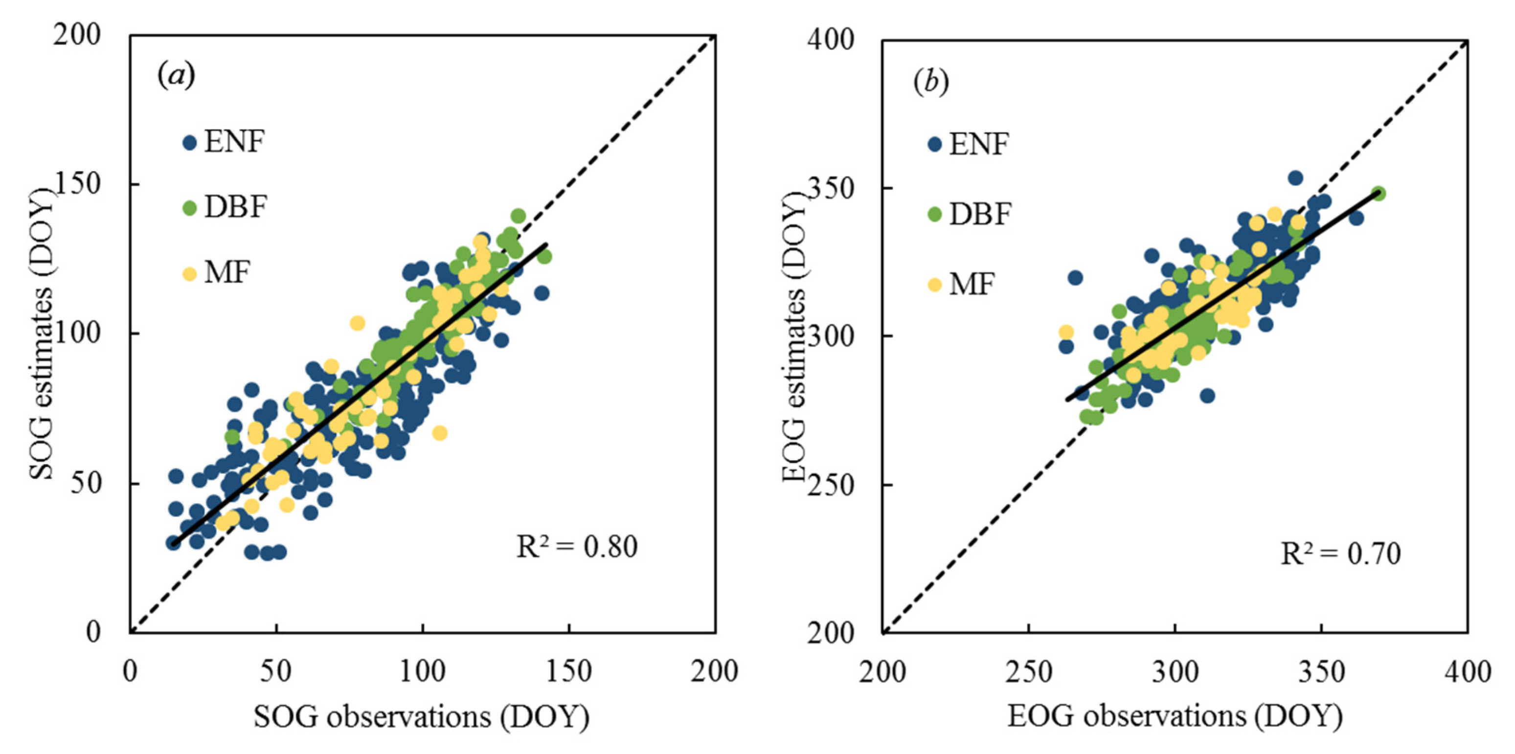
3.1. Comparison of Site-Level VPP Estimates with VPP Observations from FLUXNET GPP

The SOG and EOG estimates based on the VPPest statistical models were compared with SOG and EOG observations from daily GPP time series. For forest sites, the SOG estimates had a strong relationship with SOG observations (R2 = 0.80, p < 0.01), and the RMSE between them was 12.7 days (Figure 3 and Table 1). Agreement between the EOG estimates and EOG observations was relatively lower (R2 = 0.70, p < 0.01), but the RMSE between them (10.5 days) was comparable to that of SOG. The R2 and RMSE values between estimates and observations varied across forest types. The DBF had the highest accuracy, with R2 = 0.85 and a RMSE of less than a week for SOG, and with R2 = 0.77 and a RMSE = 7.5 days for EOG, followed by MF and ENF with a RMSE of approximately two weeks for both SOG and EOG.
The R2 values (0.78 for SOG and 0.64 for EOG) between VPP estimates and observations in non-forest sites were similar to those of forest sites, but the RMSE values (19.4 days for SOG and 22.9 days for EOG) were relatively higher than those of forest sites (Figure 4 and Table 2). The coefficients of determination between VPP estimates and observations were higher than 0.60 for all non-forest types, but the requirements for RMSE were not satisfied. The RMSE values were between two weeks and three weeks for CRO, GRA, and WET, and over three weeks for shrub sites and SAVA. The RMSE values of EOG estimates for both GRA and WET were relatively low at close to two weeks. The EOG estimates of shrub sites had the lowest R2 and the largest uncertainty with a RMSE = 39.0 days, followed by SAVA (27.5 days) and CRO (25.3 days). The SOG and EOG of non-forest types were more difficult to estimate than those of forest types.

3.2. Spatial Distribution of Global VPP Estimates

We investigated the spatial distribution of the global averaged SOG and EOG estimates for the period 2001–2017 (Figure 5a,b, respectively) as well as changes in SOG and EOG along with latitude (Figure 5c,d, respectively). Generally, the SOG decreases with a decrease in latitude, ranging from DOY 165 to DOY 80 between 85°N and 17°N, while it increases from DOY 80 to DOY 120 between 17°N and 13°N due to the arid climate of North Africa. Thereafter, it sharply decreases again from DOY 120 to DOY 65 between 13°N and the equator. In the Southern hemisphere, the SOG increases from DOY 250 at the equator to DOY 300 at 18°S, decreases from DOY 300 at 18°S to DOY 250 at 38°S, and then fluctuates between DOY 250 and DOY 300. The EOG increases with a decrease in latitude, ranging from DOY 235 at 85°N to DOY 305 at the equator. The EOG increases from DOY 130 at the equator to DOY 160 at 15°S, decreases to DOY 120 at 30°S, and then remains relatively stable from 30°S to 55°S in the Southern hemisphere.
In the Northern hemisphere, late SOG occurs at high latitudes in the mid-western United States of America, the Alps in Europe, northeast and western China, central India, and North Africa, with SOG values ranging between DOY 130 and 180. In the Southern hemisphere, late SOG occurs in northern Australia, South Africa, and southern South America, with SOG values ranging between DOY 300 and 330. Early SOG is observed in the southeastern regions of the United States of America, across the Amazon, Western Europe, Central Africa, Southeast China, and Asia. Early EOG, with values ranging from DOY 240 to DOY 280, was found at high latitudes in the mid-western United States of America, Western Europe, North China, and western India. The spatial variation in EOG in the Southern hemisphere was smaller than that in the Northern hemisphere. We found that the spatial patterns of SOG and EOG were strongly correlated with ice/snow cover, altitude, climate, and vegetation types such as CRO.

3.3. Comparisons of VPP Estimates with MODIS-LSP

Both averaged VPPest and MODIS-LSP within seven tiles (Figure S4) were compared across different PFTs for the period 2001–2017 (Table 3 and Table 4). The SOG had a strong relationship with the MODIS-SOS, except for OSH and deciduous needleleaf forest (DNF), with R < 0.5. The relationships between EOG and MODIS-EOS were relatively weaker than those between SOG and MODIS-SOS. Among all PFTs, relationships between EOG and MODIS-EOS for GRA, SVAV, MF, DBF, DNF, and WET were greater than 0.5. However, we found that the absolute bias values were relatively large for GRA, ENF, and WET in spring phenology, and for cropland/natural vegetation (CNV), WET, DNF, and ENF in autumn phenology.
The RMSD value of spring phenology for deciduous forest was the lowest of all the PFTs, with a RMSD < 10 days. For GRA and CRO, RMSD values of spring phenology were relatively large at over 20 days. The remaining PFTs had spring phenology RMSD values that ranged from 10 to 20 days. In autumn phenology, RMSD values were generally higher than in spring phenology for the majority of PFTs. Similar to spring phenology, differences between EOG and MODIS-EOS for deciduous forest were considerably smaller than other PFTs with a RMSD < 12 days. The RMSD values of autumn phenology for CRO and CNV were considerably larger than other PFTs with a RMSD > 50 days. The RMSD values in autumn phenology were 15–20 days for ENF, DNF, MF, CSH, and GRA, and 20–40 days for SAVA, SWA, and urban and built-up regions (URB). The RMSDb values were considerably smaller than the RMSD values for DNF, WET, and CRO in autumn phenology, implying that these differences are primarily associated with systematic variations.
The magnitudes of bias and RMSD between VPP and MODIS-LSP also varied across PFTs and climatic regions. For ENF, average SOG and MODIS-SOS occurred between DOY 110 and DOY 118 in H12V03, DOY 104 and DOY 117 in H12V04, and DOY 60 and DOY 88 days in H18V04, respectively (Figure 6). We found that the absolute magnitude of bias between SOG and MODIS-SOS increased for ENF, from boreal (a difference of 8 days in H12V03) to temperate in North America and the European Mediterranean region (a difference of 28 days in H18V04), whereas the magnitude of bias between EOG and MODIS-EOS increased for ENF with a decrease in latitude. Notably, spatial variations in bias between SOG and MODIS-SOS for MF were considerable. For MF, average SOG and MODIS-SOS were detected at DOY 142 and DOY 124 in H23V02, DOY 124 and DOY 120 in H12V04, and DOY 5 and DOY 72 in H20V08, respectively. A considerably large bias between SOG and MODIS-SOS occurred for MF in humid tropical regions (H20V08).
The average SOG for DBF ranged from DOY 96 to DOY 117 and occurred 4–7 days later than the MODIS-SOS, which ranged from DOY 89 to DOY 113 in temperate and European Mediterranean regions (H12V04, H18V04, and H27V05). However, the average SOG in tropical humid regions (H20V08) occurred on DOY 88, 18 days later than the MODIS-SOS (DOY 70). The magnitude of bias between SOG and MODIS-SOS increased for DBF with a decrease in latitude, implying that the difference between SOG and MODIS-SOS in tropical regions was larger than that in temperate regions.
The spatial variations in bias between SOG and MODIS-SOS, and between EOG and MODIS-EOS, for CRO were also very clear. A large bias between SOG and MODIS-SOS was found for CRO in arid tropical regions (H20V07), while a large bias between EOG and MODIS-EOS was found for CRO in arid tropical and temperate Asian regions. The SOG (DOY 109) was clearly biased and occurred earlier than the MODIS-SOS (DOY 169), while the EOG (DOY 271) also occurred earlier than the MODIS-EOS (DOY 325) in arid tropical regions for CRO. A large discrepancy between SOG and MODIS-SOS was also found for GRA. The SOG (DOY 148) was earlier than the MODIS-SOS (DOY 174), and there was no bias between EOG (DOY 319) and the MODIS-EOS (DOY 319) in arid tropical regions for GRA.
For the majority of PFTs, the bias between VPP and MODIS-LSP was larger in the European Mediterranean region (H18V04 tile) than in temperate and boreal North America and Subarctic Eurasia. Furthermore, our results show large discrepancies between VPP and MODIS-LSP in the European Mediterranean region and in arid and humid tropical regions compared with temperate and boreal North America and Subarctic Eurasia.

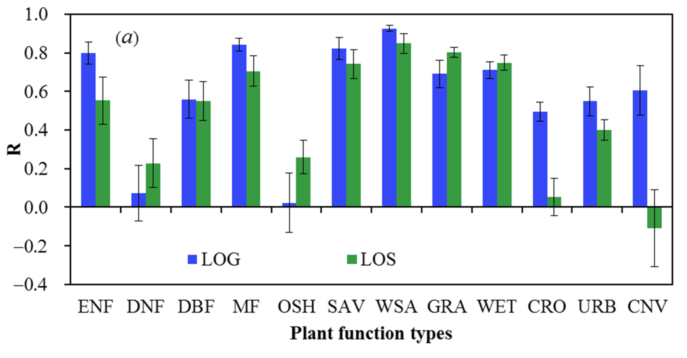
3.4. Relationship between VPP, MODIS-LSP, and GPP

We further compared the relationships of LOG and LOS estimates to two individual global GPP products (GPPVPM from the VPM model and GLASS-GPP from the EC-LUE model) across all PFTs from 2001 to 2016, based on the data within the seven tiles (Figure 7 and Figure S5). The results show that LOG estimates were more closely related to annual GPP than LOS for most PFTs. The R-values of ENF, MF, SVAV, and WVA were above 0.8 using LOG estimates, while only those of WVA and GRA were above 0.8 using LOS. Eight of thirteen PFTs had higher R values (ENF, MF, SAVA, WVA, CRO, URB, and CNV) using LOG estimates compared with those using LOS, while the R values for DNF, OSH, and GRA were lower using LOG estimates than those using LOS. The R-value of WET from LOG estimates was lower than that from LOS estimates for GPPVPM, but the R-value of WET from LOG estimates was higher than that from LOS estimates for GLASS-GPP. There was no significant difference in R-values between LOG and LOS estimates for DBF. The R-values of CRO and CNV using LOG estimates were noticeably higher than those using LOS. The relationship between LOS and annual GPP for CRO and CNV was negative and not significant. These results are consistent with those based on the FLUXNET data. The ability to explain annual GPP was improved when LOS was replaced by LOG for all PFTs.

4. Discussion

4.1. Accuracy of Site-Level VPP Estimates across PFTs

The estimation accuracy of both SOG and EOG varied across forest types. Consistent with results from previous studies [17], our results indicate that the VPP for deciduous forest was detected more accurately than that for evergreen forest due to the relatively dramatic seasonal variation in canopy greenness. The accuracy of VPP for MF was medium between DBF and ENF. The results further indicate that the performance of phenology modeling based on vegetation indices largely depends on the variability in canopy greenness. Previous studies showed that the individual use of vegetation indices did not accurately predict LSP of ENF because of stable changes in seasonal canopy greenness [24].
The importance of temperature in improving phenology modeling for ENF has been investigated in a number of studies [7,24]. Temperature is the most important driving factor of photosynthetic activity for ENF and MF because these are primarily distributed in boreal and temperate regions (Figure S6). Therefore, the accuracy of VPP estimates for MF and ENF was clearly improved by including temperature as a variable in VPP modeling.
Compared with forest types, our results indicate that VPP modeling for non-forest types is more challenging, probably due to the higher heterogeneity, sensitivity to climate change, disturbance, and the human management involved in non-forest types [2,50]. Highly heterogeneous SAVA and OSH include more than two types of plant species, resulting in complicated phenology phases [2]. For example, SAVA consists of mixed grasses and trees, while temporal differences in EOS between these two vegetation types reached three months [2,51]. Different plant species with the same eddy covariance footprint will vary in their contribution to carbon uptake, making it difficult to predict the phenological cycle of an ecosystem as a whole [16,52]. Furthermore, increasing the spatial complexity of ecosystems within a MODIS pixel area reduces the ability of vegetation indices to explain carbon flux and be used for further VPP modeling [16]. The spectral signatures of CRO and GRA are usually combined with soil and vegetation at the beginning and end of the growing season, owing to the low presence of vegetation, while the EVI is less sensitive to changes in soil background [16,53]. Thus, other vegetation indices with a strong ability to minimize the effect of the soil background may be more suitable for predicting phenology than the EVI for CRO and GRA [16]. Additionally, the variability in phenology of CRO is significantly influenced by human management, and there are large differences in phenology between single and double cropping patterns [54,55,56]. Furthermore, GRA is more sensitive to climate and human disturbance [57,58], which causes multiple factor effects on variations in VPP for GRA. All of these reasons result in high complexity and uncertainty in the modeling of VPP for non-forest types.

4.2. Discrepancies between VPP Estimates from the Regression Models and MODIS-LSP

Comparing MODIS-LSP and VPP estimates using the same threshold (15% of the amplitude), we found considerable differences that varied across PFTs. The discrepancies (RMSD) ranged from 10 to 25 days between SOG and MODIS-SOS, and from 11 to 62 days between EOG and MODIS-EOS, depending on PFTs. This is confirmed by previous studies that indicated significant temporal lags between MODIS EVI-derived LSP and VPP [11,59], and between LSP from in situ measured green indices and VPP [11,60].
MODIS-LSP showed good agreement and synchronization with VPP with high correlations and low random differences (RMSDb) for DBF, which is consistent with previous studies [7,11,16,49]. Results from these studies indicate that the photosynthetic activity is closely related to greening and coloring of leaves for deciduous forests [7,11,16]. Leaf emergence is triggered by cumulative temperature at the start of season and leaf senescence is controlled by minimum temperature at the end of the season [61]. Hence, strong linkages and synchronizations among photosynthetic activity, leaf activity, and variations in temperature result in a close relationship between LSP and VPP for deciduous forests.
We found that the bias between MODIS-LSP and VPP varied among PFTs and climatic regions. Spring photosynthetic phenology occurred later than EVI-derived spring phenology, and autumn photosynthetic phenology occurred earlier than EVI-derived autumn phenology for DBF. Previous studies showed that the SOG occurs approximately one week later than the EVI-derived SOS, and EOG occurs approximately two weeks earlier than the EVI-derived EOS for DBF [11,49]. Physiological capacity, such as maturation of chlorophyll and Rubisco enzymes, does not end after leaf expansion [11,62]. The start of photosynthetic capacity in beech trees during spring occurred with an observed lag after leaf expansion [11,16,63,64]. Furthermore, for some deciduous trees leaves in the inner part of the canopy start changing their color earlier than at the top part of canopy [11,65], which results in disagreement between remote sensing observations and photosynthetic capacity. All of these physiological phenomena explain the temporal lags between VPP and MODIS-LSP for deciduous forests.
However, the large negative bias between SOG from the regression models and the MODIS-SOS for ENF indicates that the SOG occurred earlier than the MODIS-SOS, which is consistent with results from [66,67]. Vegetation-indices-derived SOS occurred 50 days late relative to the timing of 5% GPP [66], and 25 days later in high-latitude regions for ENF [67]. For evergreen forests, the positive bias between EOG and MODIS-EOS for ENF indicates that the EOG occurred later than the MODIS-EOS. Photosynthetic phenology in evergreen forests has no correlation with vegetation-indices-derived LSP because the VPP of evergreen forests is more related to climatic factors than canopy greenness and physiological activity is decoupled from changes in greenness [16]. Physiological activity is likely to start early in spring and continue to the end of the season if climatic conditions are still favorable [11]. The greenness of evergreen understory vegetation is barely detectable by optical remote sensing, and the carbon uptake contributed by evergreen understory vegetation will make the SOG occur earlier than the SOS and the EOG occur later than the EOS, which also results in lags and discrepancies between LSP and VPP [11]. The discrepancies between VPP and the MODIS-LSP for MF were more complex than those for ENF and DBF. The temporal lags between VPP and the MODIS-LSP for MF are similar to those of DBF at high latitudes and evergreen forest at low latitudes. When the fraction of snow cover is low during the snowmelt process, greenness can be detected by remote sensing data; however, photosynthesis is weak due to unsuitable temperatures. This may be a reason for the fact that the SOG of MF occurred later than the MODIS-SOS in subarctic regions.
Spatial variations in bias and RMSD between VPP and MODIS-LSP were relatively high across the same PFT. The bias between MODIS-LSP and VPP also varied across climatic regions. The bias was larger in tropical regions than in boreal and temperate regions for forest types. Similar findings were also obtained by [66], who showed that the bias between SOG and the MODIS-SOS for ENF in the Mediterranean region with a humid and warm climate was greater than that in the boreal and temperate regions. Joint controls of climatic forcing and canopy greenness result in differences between VPP and MODIS-LSP across climatic regions. Discrepancies between VPP and MODIS-LSP for evergreen and deciduous forests in subarctic, boreal, and temperate regions were relatively low, due to temperature being a major climatic factor influencing both VPP and MODIS-LSP for deciduous forests in these regions [68]. The MODIS-SOS was detected at the time of recovery of pigments in old leaves and the emergence of new leaves for evergreen forest when the temperature was suitable for the start of photosynthesis [66]. Additionally, snow cover has an important influence on spring and autumn phenology [69], and the date of snowmelt may result in a shortening of the temporal lags between SOG and the MODIS-SOS in high-latitude regions [42,66], as leaves emerge directly after snowmelt [45]. In tropical regions, variations in photosynthetic carbon uptake primarily depend on climatic forcing rather than canopy greenness [16,70], and this variation is not reflected by remote sensing data [16,71]. This causes the random difference between VPP and the MODIS-LSP to be relatively high for evergreen forests in tropical regions.
Spatial variations in discrepancies between VPP and MODIS-LSP for non-forest types are relatively smaller but more complex than those for forest types, and primarily occur in CRO and GRA in arid tropical and temperate Asian regions due to the extreme climatic conditions [72] and human land use management [73]. The bias between VPP and LSP in arid tropical regions was larger than those in temperate North America and the European Mediterranean region for CRO and GRA. Water and heat stress result in a decoupling of vegetation greenness and photosynthetic capacity [74], which causes the discrepancy between VPP and MODIS-LSP in arid regions, especially for evergreen plants. High variation in MODIS-SOS and MODIS-EOS for CRO was observed in northern Africa (an arid tropical region), with SOS ranging from June to October and EOS ranging from June to November [56]. The MODIS-LSP is more similar to results from [56] than VPP estimates, implying that there may be large uncertainty in VPP estimates for CRO in arid tropical regions. A large bias between SOG and MODIS-SOS for GRA in arid tropical regions was also observed. The SOG (DOY 144–151) for GRA was more similar to the spring phenology (early June, approximately DOY 151–160) from [56] in northern Africa than the MODIS-SOS (DOY 160–190). Both averaged EOG (DOY 315–324) and MODIS-EOS (DOY 309–330) for GRA were similar to the results (DOY 300–330) from [56] in northern Africa. This comparison shows that the SOG and EOG estimates for GRA in arid tropical regions were relatively reliable.
The averaged SOG (DOY 100) was comparable to the averaged MODIS-SOS (DOY 96) for temperate Asia and both were within the range from DOY 90 to 120 for CRO [54]. The averaged EOG (DOY 279) for CRO occurred later than the averaged MODIS-EOS (DOY 252) for temperate Asia and was closer to the results of [54] (DOY 270 to 300) than that of MODIS-EOS. Agricultural land management is a major reason for the large random differences between MODIS-LSP and VPP for CRO in temperate Asia [54]. In addition, the cropping patterns have a clear difference between temperate Asia and North America [54,75]. The majority of agricultural land in temperate Asia has multiple cropping patterns [54], while the majority of agricultural land in temperate North America and European Mediterranean region has a single cropping pattern [75]. Therefore, the complex phenology for CRO with multiple cropping patterns in temperate Asia results in large random differences between VPP and MODIS-LSP.

4.3. Limitations of the Method

Vegetation phenology monitoring based on remote sensing data faces major challenges for non-forest types and for high latitude, arid, and humid tropical regions [47]. In this study, we found that snow cover information, such as snow cover periods from MOD13C1 products, is strongly correlated with spring and autumn phenology. Considering snow cover information as a variable in the model improves the accuracy of spring and autumn phenology estimates in high-latitude regions. However, the statistical models proposed in this study for estimating vegetation phenology may have a number of uncertainties for arid and humid tropical regions because only a few FLUXNET sites located in these regions can be used for model calibration. The method proposed in this study only considers temperature as a major climate factor for VPP estimation. On the other hand, the photosynthetic capability has a weak relationship with temperature, and is primarily regulated by radiation, precipitation, and available soil water content in arid and humid tropical regions [76].
On a global scale, growing seasons for vegetation in different climatic zones are diverse. For example, in the majority of the evergreen forests in humid tropical regions the growing season begins in the preceding year or ends in the following year [56]. Furthermore, some vegetation types in arid regions have multiple and variable growing seasons depending on the variation in temperature in the early months and precipitation in the mid growing season [72]. Considering these specific situations will further improve the model and the method used to decrease uncertainties of VPP estimates in arid and humid tropical regions. The CRO is a special vegetation type and its phenology is largely determined by the cropping pattern of land management. The method proposed in this study has the ability of exacting VPP for CRO with a single cropping pattern but does not allow for the exacting of all start and end dates of growing seasons for CRO with multiple growing seasons. Exacting VPP of CRO with multiple cropping patterns could be the third improvement of the method to increase the accuracy of VPP estimates for CRO.

5. Conclusions

Our results show that VPP was accurately estimated with a RMSE of approximately two weeks for forest types and three weeks for non-forest types through a combination of MODIS EVI and LST using a series of PFT-specific statistical models. Accurately estimating the VPP for non-forest types was more challenging than for forest types, primarily due to the high heterogeneity and human disturbances in non-forest types. We suggest that methods that are more effective be developed for improving VPP estimation of those PFTs with complicated seasonal variations in photosynthetic carbon uptake, such as multiple growing seasons, as well as SOG and EOG in the preceding year or in the following year. The dates of snow/ice cover used in this study played a useful role, to some extent, in constraining and improving the VPP estimates in high-latitude regions.
The VPP is not identical to LSP, and the bias between VPP and LSP varied across PFTs and climate regions. High agreement between VPP and LSP from different data sources was found for DBF, although systematic differences were present. The spring photosynthetic phenology occurred slightly later than SOS, while the autumn photosynthetic phenology occurred slightly earlier relative to EOS for DBF. The sign of bias between VPP and LSP for ENF was opposite to that of DBF, with SOG occurring earlier than SOS and EOG occurring later than EOS. Generally, for forest types, the bias between VPP and LSP was larger in warm and humid regions than in cold high-latitude and high-altitude regions. Climatic factors and canopy greenness jointly controlled spatial variations in discrepancies between VPP and LSP.
Discrepancies between VPP and LSP for non-forest types were more complicated than those for forest types. High discrepancies between VPP and LSP were found in arid tropical and temperate Asian regions for CRO and GRA due to their sensitivity to extreme climatic conditions and the intensive management of planting and grazing. The method proposed in this study failed to extract the VPP of CRO with multiple cropping patterns and other vegetation types with multiple growing seasons triggered by alternating drought and precipitation periods.
A stronger correlation was found between LOG from VPP estimates and GPP than that between LOS from LSP estimates and GPP for the majority of PFTs, especially for ENF and CRO. The VPP estimates mapped in this study provided a carbon-objective vegetation phenology and optimized the vegetation phenology module of land surface models. This improves the estimates of carbon and water exchange between the atmosphere and terrestrial ecosystem and enhances our understanding of the relationship and feedback between vegetation and climate under current and future climate change.

Supplementary Materials

The following are available online at https://0-www-mdpi-com.brum.beds.ac.uk/article/10.3390/rs13245080/s1. Figure S1: An example shows how starting and ending days of GPP (SOG and EOG, respectively), and GPPmax are derived from daily GPP time series; multi-years averaged daily GPP are indicated with black circle, and solid red line are smoothed daily GPP; 15% amplitude threshold dates are indicated with vertical lines; minimum (GPPmin) and maximum (GPPmax) of smoothed daily GPP are indicated with horizontal lines. Data are averaged daily GPP from 2000-2014 for the FLUXNET site US- UMB (deciduous broadleaf forest), Figure S2: Spatial distribution of quality assurance values for (a) starting day of GPP (SOG) and (b) ending day of GPP (EOG) in 2014, Figure S3: Sinusoidal MODIS Tile Grid shown in https://modis-land.gsfc.nasa.gov/MODLAND_grid.html (accessed on 20 May 2021), Figure S4: Spatial patterns of the averaged vegetation photosynthetic phenology (VPP) and MODIS-LSP from 2001 to 2017 for the seven selected tiles. Row represents different tiles. Column represents different VPP and MODIS-LSP. Row1 is H12V03, Row2 is H12V04, Row3 is H18V04, Row4 is H20V07, Row5 is H20V08, Row6 is H23V02, and Row7 is H27V05. Column1 is starting day of GPP (SOG), Column2 is MODIS-SOS, Column3 is ending day of GPP (EOG), and Column4 is MODIS-EOS. Location information for these tiles can be found in Fig.S3, Figure S5: Relationships between length of photosynthesis phenology season (LOG) and annual GPP from the VPM model (Left) and between LOS and annual GPP from the VPM model (Right) for different plant functional types in 2014. Evergreen needle-leaf forest (ENF), deciduous needleleaf forest (DNF), deciduous broadleaf forest (DBF), mixed forest (MF), open shrublands (OSH), savannas (SAV), woody savannas (WSA), grasslands (GRA), wetlands (WET), croplands (CRO), urban and built-up (URB), and cropland/natural vegetation (CNV), Figure S6: Changes in number of pixels along with latitude for different forest types: evergreen needle-leaf forest (ENF), evergreen broadleaf forest (EBF), deciduous broadleaf forest (DBF), and mixed forest (MF), Table S1: Total 145 eddy covariance sites across the northern hemisphere used in this study. Site descriptions include Site Identifier (ID), Latitude (Lat, ◦), Longitude (Lon, ◦), Plant Functional Type (PFT), Period of Record, and a reference for each site. PFTs are taken from the International Geosphere-Biosphere Program (IGBP) land cover classification scheme. evergreen needle-leaf forest (ENF), deciduous broadleaf forest (DBF), mixed forest (MF), closed shrublands (CSH), open shrublands (OSH), savannas (SAV), woody savannas (WSA), grasslands (GRA), wetlands (WET), and croplands (CRO). Please find more information from http://fluxnet.fluxdata.org/ (accessed on 20 May 2021), Table S2: Detailed descriptions of the twenty-eight variables derived from smoothed MODIS EVI and LST data.

Author Contributions

Conceptualization, X.X. and J.H.; methodology, X.X.; validation, X.X. and Y.T.; data curation, X.X., Y.T., Z.Z. and Y.Q.; writing—original draft preparation, X.X. and Y.T.; writing—review and editing, X.X. and J.H.; funding acquisition, X.X. and J.H. All authors have read and agreed to the published version of the manuscript.

Funding

This research was supported by the Natural Science Foundation of Zhejiang Province (grant No. LY21C030001) and the National Natural Science Foundation of China (Grant Nos. 31870619, 31570629).

Institutional Review Board Statement

Not applicable for studies not involving humans.

Informed Consent Statement

Not applicable for studies not involving humans or animals.

Data Availability Statement

The data that support the findings of this study are available from the author upon reasonable request.

Acknowledgments

This work used eddy covariance data acquired and shared by the FLUXNET community, including these networks: AmeriFlux, AfriFlux, AsiaFlux, CarboAfrica, CarboEuropeIP, CarboItaly, CarboMont, ChinaFlux, Fluxnet-Canada, GreenGrass, ICOS, KoFlux, LBA, NECC, OzFlux-TERN, TCOS-Siberia, and USCCC. The ERA-Interim reanalysis data were provided by ECMWF and processed by LSCE. The FLUXNET eddy covariance data processing and harmonization were carried out by the European Fluxes Database Cluster, the AmeriFlux Management Project, and the Fluxdata project of FLUXNET, with the support of the CDIAC and ICOS Ecosystem Thematic Center and the OzFlux, ChinaFlux, and AsiaFlux offices. The authors thank the three anonymous reviewers for their valuable comments that helped to improve the quality of this paper.

Conflicts of Interest

The authors declare no conflict of interest.

Abbreviations

LSPLand surface phenology
MODIS-LSP  Land surface phenology downloaded from the MODIS dataset
SOSStart of growing season, refers to MODIS-SOS
EOSEnd of growing season, refers to MODIS-EOS
LOSLength of growing season, equals EOS minus SOS, and refers to
MODIS-LOS
VPPVegetation photosynthetic phenology, implying the key transitions
of vegetation carbon fluxes
VPP obsVPP derived from the FLUXNET daily gross primary productivity
(GPP) data
VPP estVPP estimated based on the relationship between VPP observations
and MODIS products using the regression models
SOGStarting days of GPP, from VPPobs or VPPest
EOGEnding days of GPP, from VPPobs or VPPest
LOGLength of the photosynthetic phenology season, equal to EOG minus SOG.

Appendix A

Table A1. Model formulas for estimating the starting days of GPP (SOG). Evergreen needle-leaf forest (ENF), deciduous broadleaf forest (DBF), mixed forest (MF), closed shrublands (CSH), open shrublands (OSH), savannas (SAV), woody savannas (WSA), grasslands (GRA), wetlands (WET), and croplands (CRO). sp, spring; su, summer; au, autumn, m, mean; max, maximal; s, standard deviation; and c, coefficient of variation. For example, mEVIsp is the mean enhanced vegetation index (EVI) during spring. The number after EVI or LST means the day of the year (DOY); for example, EVI243 is the EVI value at DOY234. The full names for independent variables can be found in Table S2.
Plant Function TypesModel Formula
ForestENFSOG = 684.40 − 115.13 × mEVIsp − 165.15 × sEVIsp + 70.16 × EVI243 − 2.09 × LST60
DBFSOG = 237.01 − 116.82 × mEVIsp + 86.70 × mEVIsu − 0.43 × LST243
DNF
MFSOG = −73.94 − 94.49 × EVI334 − 2.20 × LST60 + 2.77 × mLSTsu − 2362.37 × cLSTsu
Non-forestCSHSOG = −51.57 − 243.87 × mEVIsp + 117.05 × EVI243 + 2.88 × LST152 − 2.30 × LST243 + 221.19 × sEVIsu
OSH
SAV
WSA
GRASOG = 180.18 − 180.55 × mEVIsp + 207.39 × sEVIsu − 3.25 × sLSTau
CROSOG = 88.28 − 114.86 × mEVIsp + 141.83 × maxEVIsu
−51.35 × EVI152
WETSOG = 521.47 − 1.40 × mLSTsp + 352.64 × sEVIsu − 62.34 × mEVIsp

Appendix B

Table A2. Model formulas for estimating the ending days of GPP (EOG). Evergreen needle-leaf forest (ENF), deciduous broadleaf forest (DBF), mixed forest (MF), closed shrublands (CSH), open shrublands (OSH), savannas (SAV), woody savannas (WSA), grasslands (GRA), wetlands (WET), and croplands (CRO). sp, spring; su, summer; au, autumn; m, mean; max, maximal; s, standard deviation; and c, coefficient of variation. For example, mEVIsp is the mean enhanced vegetation index (EVI) during spring. The number after EVI or LST means the day of the year (DOY); for example, EVI243 is the EVI value at DOY234. The full names for independent variables can be found in Table S2.
Plant Function TypesModel Formula
ForestENFEOG = −1.80 + 40.66 × mEVIsp + 175.16 × sEVIsp − 1.47 × maxLSTsu + 2.51 × mLSTau
DBF
DNF
EOG = −82.16− 15.40 × EVI152 + 98.14 × mEVIau + 1.17 × mLSTau
MFEOG = −287.59 + 52.09 × mEVIsp + 1.93 × mLSTau
Non-forestCSH
OSH
SAV
WSA
EOG =459.51 + 149.45 × mEVIau + 2.40 × LST152 − 1.71 × LST243 + 2.84 × mLSTsp
−6.31 × mLSTau + 2.05 × LST334 − 58.60 × mEVIsp
GRAEOG = 290.49 − 10.46 × sEVIsu + 48.94 × mEVIau + 501.01 × cLSTsp − 6.02 × sLSTau
CROEOG = 208.56 + 189.10 × EVI243 − 185.12 × EVI152 + 390.12 × sEVIsp-362.92 × sEVIau + 59.43 × mEVIsu
WETEOG = −400.64 + 1.15 × LST334 − 175.05 × sEVIsp + 1.28 × LST243

References

  1. Friedl, M.; Henebry, G.M.; Reed, B.; Huete, A.; White, M.; Morisette, J.; Nemani, R.; Zhang, X.; Myneni, R. Land Surface Phenology. A Community White Paper Requested by NASA. 2006. Available online: https://lcluc.umd.edu/documents/friedl-m-g-henebry-b-reed-huete-m-white-j-morisette-r-nemani-x-zhang-and-r-myneni-2006 (accessed on 15 May 2021).
  2. Zhang, X.; Liu, L.; Liu, Y.; Jayavelu, S.; Wang, J.; Moon, M.; Henebry, G.M.; Friedl, M.A.; Schaaf, C.B. Generation and evaluation of the VIIRS land surface phenology product. Remote Sens. Environ. 2018, 216, 212–229. [Google Scholar] [CrossRef]
  3. Keenan, T.F.; Gray, J.; Friedl, M.A.; Toomey, M.; Bohrer, G.; Hollinger, D.Y.; Munger, J.M.; O’Keefe, J.; Schmid, H.P.; Wing, I.S.; et al. Net carbon uptake has increased through warming-induced changes in temperate forest phenology. Nat. Clim. Chang. 2014, 4, 598–604. [Google Scholar] [CrossRef]
  4. Xia, J.; Niu, S.; Ciais, P.; Janssens, I.A.; Chen, J.; Ammann, C.; Arain, A.; Blanken, P.D.; Cescatti, A.; Bonal, D.; et al. Joint control of terrestrial gross primary productivity by plant phenology and physiology. Proc. Natl. Acad. Sci. USA 2015, 112, 2788–2793. Available online: http://ir.itpcas.ac.cn/handle/131C11/7356 (accessed on 20 May 2021). [CrossRef] [PubMed] [Green Version]
  5. Zhang, X.; Friedl, M.A.; Schaaf, C.B.; Strahler, A.H.; Hodges, J.C.F.; Gao, F.; Reed, B.C.; Huete, A. Monitoring vegetation phenology using MODIS. Remote Sens. Environ. 2003, 84, 471–475. [Google Scholar] [CrossRef]
  6. Zhang, X.; Friedl, M.A.; Schaaf, C.B. Global vegetation phenology from moderate resolution imaging spectroradiometer (MODIS): Evaluation of global patterns and comparison with in situ measurements. J. Geophys. Res. Biogeosci. 2006, 111, G04017. [Google Scholar] [CrossRef]
  7. Gonsamo, A.; Chen, J.M.; Wu, C.; Dragoni, D. Predicting deciduous forest carbon uptake phenology by upscaling FLUXNET measurements using remote sensing data. Agric. For. Meteorol. 2012, 165, 127–135. [Google Scholar] [CrossRef]
  8. Richardson, A.D.; Hufkens, K.; Milliman, T.; Aubrecht, D.M.; Frolking, S. Tracking vegetation phenology across diverse North American biomes using phenocam imagery. Sci. Data 2018, 5, 180028. [Google Scholar] [CrossRef]
  9. Zhang, X.; Wang, J.; Gao, F.; Liu, Y.; Schaaf, C.; Friedl, M.; Yu, Y.; Jayavelu, S.; Gray, J.; Liu, L.; et al. Exploration of scaling effects on coarse resolution land surface phenology. Remote Sens. Environ. 2017, 190, 318–330. [Google Scholar] [CrossRef] [Green Version]
  10. Richardson, A.D.; Black, T.A.; Ciais, P.; Delbart, N.; Friedl, M.A.; Gobron, N.; Hollinger, D.Y.; Kutsch, W.L.; Longdoz, B.; Luyssaert, S.; et al. Influence of spring and autumn phenological transitions on forest ecosystem productivity. Philos. Trans. R. Soc. Lond. 2010, 365, 3227–3246. [Google Scholar] [CrossRef] [PubMed] [Green Version]
  11. D’Odorico, P.; Gonsamo, A.; Gough, C.M.; Bohrer, G.; Morison, J.; Wilkinson, J.; Hanson, P.J.; Gianelle, D.; Fuentes, J.D.; Buchmann, N. The match and mismatch between photosynthesis and land surface phenology of deciduous forests. Agric. For. Meteorol. 2015, 214–215, 25–38. [Google Scholar] [CrossRef]
  12. Wang, X.; Xiao, J.; Li, X.; Cheng, G.; Ma, M.; Zhu, G.; Mehnaz, A.; Black, T.; Rachhpal, J. No trends in spring and autumn phenology during the global warming hiatus. Nat. Commun. 2019, 10, 2389. [Google Scholar] [CrossRef] [PubMed]
  13. Yang, L.; Noormets, A. Standardized flux seasonality metrics: A companion dataset for FLUXNET annual product. Earth Syst. Sci. Data Discuss. 2020, 13, 1461–1475. [Google Scholar] [CrossRef]
  14. Gonsamo, A.; Chen, J.M.; D’Odorico, P. Deriving land surface phenology indicators from CO2 eddy covariance measurements. Ecol. Indic. 2013, 29, 203–207. [Google Scholar] [CrossRef]
  15. Wu, C.; Chen, J.M.; Gonsamo, A.; Price, D.T.; Black, T.A.; Kurz, W.A. Interannual variability of net carbon exchange is related to the lag between the end-dates of net carbon uptake and photosynthesis: Evidence from long records at two contrasting forest stands. Agric. For. Meteorol. 2012, 164, 29–38. [Google Scholar] [CrossRef]
  16. Balzarolo, M.; Vicca, S.; Nguy-Robertson, A.L.; Bonal, D.; Elbers, J.A.; Fu, Y.H.; Grünwald, T.; Horemans, J.A.; Papale, D.; Peñuelas, J.; et al. Matching the phenology of Net Ecosystem Exchange and vegetation indices estimated with MODIS and FLUXNET in-situ observations. Remote Sens. Environ. 2016, 174, 290–300. [Google Scholar] [CrossRef] [Green Version]
  17. Wu, C.; Peng, D.; Soudani, K.; Siebicke, L.; Gough, C.M.; Arain, M.A.; Bohrer, G.; Lafleur, P.M.; Gonsamo, A.; Xu, S.; et al. Land surface phenology derived from normalized difference vegetation index (NDVI) at global FLUXNET sites. Agric. For. Meteorol. 2017, 233, 171–182. [Google Scholar] [CrossRef]
  18. Richardson, A.D.; Keenan, T.F.; Migliavacca, M.; Ryu, Y.; Sonnentag, O.; Toomey, M. Climate change, phenology, and phenological control of vegetation feedbacks to the climate system. Agric. For. Meteorol. 2013, 169, 156–173. [Google Scholar] [CrossRef]
  19. Gonsamo, A.; Croft, H.; Chen, J.M.; Wu, C.; Froelich, N.; Staebler, R.M. Radiation contributed more than temperature to increased decadal autumn and annual carbon uptake of two eastern North America mature forests. Agric. For. Meteorol. 2015, 201, 740–749. [Google Scholar] [CrossRef]
  20. Fu, Z.; Stoy, P.C.; Luo, Y.; Chen, J.; Sun, J.; Montagnani, L.; Wohlfahrt, G.; Rahman, F.; Rambal, S.; Bernhoferet, C.; et al. Climate controls over the net carbon uptake period and amplitude of net ecosystem production in temperate and boreal ecosystems. Agric. For. Meteorol. 2017, 243, 9–18. [Google Scholar] [CrossRef] [Green Version]
  21. Garrity, S.R.; Bohrer, G.; Maurer, K.D.; Mueller, K.L.; Vogel, C.S.; Curtis, P.S. A comparison of multiple phenology data sources for estimating seasonal transitions in deciduous forest carbon exchange. Agric. For. Meteorol. 2011, 151, 1741–1752. [Google Scholar] [CrossRef]
  22. Chen, B.; Che, M. Improving vegetation phenological parameterization of, a land surface model. Biogeosc. Discuss. 2016. preprint. [Google Scholar] [CrossRef]
  23. Peng, B.; Guan, K.; Chen, M.; Lawrence, D.M.; Pokhrel, Y.; Suyker, A.; Arkebauer, T.; Lu, Q. Improving maize growth processes in the community land model: Implementation and evaluation. Agric. For. Meteorol. 2018, 250–251, 64–89. [Google Scholar] [CrossRef]
  24. Liu, Y.; Wu, C.; Peng, D.; Xu, S.; Gonsamo, A.; Jassal, R.S.; Arain, M.A.; Lu, L.; Fang, B.; Chen, M. Improved modeling of land surface phenology using MODIS land surface reflectance and temperature at evergreen needleleaf forests of central North America. Remote Sens. Environ. 2016, 176, 152–162. [Google Scholar] [CrossRef]
  25. Reichstein, M.; Falge, E.; Baldocchi, D.; Papale, D.; Valentini, R. On the Separation of Net Ecosystem Exchange into Assimilation and Ecosystem Respiration: Review and Improved Algorithm. Glob. Chang. Biol. 2005, 11, 1424–1439. [Google Scholar] [CrossRef]
  26. Papale, D.; Reichstein, M.; Aubinet, M.; Canfora, E.; Bernhofer, C.; Kutsch, W.; Longdoz, B.; Rambal, S.; Valentini, R.; Vesala, T.; et al. Towards a standardized processing of Net Ecosystem Exchange measured with eddy covariance technique: Algorithms and uncertainty estimation. Biogeosciences 2006, 3, 571–583. [Google Scholar] [CrossRef] [Green Version]
  27. Lasslop, G.; Reichstein, M.; Papale, D.; Richardson, A.D.; Arneth, A.; Barr, A.; Paul, S.; Gerog, W. Separation of net ecosystem exchange into assimilation and respiration using a light response curve approach: Critical issues and global evaluation. Glob. Chang. Biol. 2010, 16, 187–208. [Google Scholar] [CrossRef] [Green Version]
  28. Belward, A.S.; Estes, J.E.; Kline, K.D. The IGBP-DIS 1-Km Land-Cover Data Set DISCover: A Project Overview. Photogramm. Eng. Remote Sens. 1999, 65, 1013–1020. [Google Scholar]
  29. Chen, J.; Jönsson, P.; Tamura, M.; Gu, Z.; Matsushita, B.; Eklundh, L. A simple method for reconstructing a high-quality NDVI time-series data set based on the Savitzky-Golay filter. Remote Sens. Environ. 2004, 91, 332–344. [Google Scholar] [CrossRef]
  30. Pan, Z.K.; Huang, J.F.; Zhou, Q.B.; Wang, L.M.; Cheng, Y.X.; Zhang, H.K.; Blackburn, G.A.; Yan, J.; Liu, J.H. Mapping Crop Phenology Using NDVI Time-Series Derived from HJ-1 A/B Data. Int. J. Appl. Earth Obs. Geoinf. 2015, 34, 188–197. [Google Scholar] [CrossRef] [Green Version]
  31. Xu, X.; Zhou, G.; Du, H.; Mao, F.; Xu, L.; Li, X.; Liu, L. Combined MODIS land surface temperature and greenness data for modeling vegetation phenology, physiology, and gross primary production in terrestrial ecosystems. Sci. Total Environ. 2020, 726, 137948. [Google Scholar] [CrossRef]
  32. Zhou, S.; Zhang, Y.; Caylor, K.K.; Luo, Y.; Xiao, X.; Ciais, P.; Huang, Y.; Wang, G. Explaining inter-annual variability of gross primary productivity from plant phenology and physiology. Agric. For. Meteorol. 2016, 226–227, 246–256. [Google Scholar] [CrossRef] [Green Version]
  33. Cong, N.; Wang, T.; Nan, H.; Ma, Y.; Wang, X.; Myneni, R.B.; Piao, S. Changes in satellite-derived spring vegetation green-up date and its linkage to climate in china from 1982 to 2010: A multimethod analysis. Glob. Chang. Biol. 2013, 19, 881–891. [Google Scholar] [CrossRef]
  34. Gray, J.; Sulla-Menashe, D.; Friedl, M. MCD12Q2 MODIS/Terra+Aqua Land Cover Dynamics Yearly L3 Global 500m SIN Grid V006; NASA EOSDIS Land Processes DAAC: Sioux Falls, SD, USA, 2019. [CrossRef]
  35. Sims, D.A.; Rahman, A.F.; Cordova, V.D.; El-Masri, B.Z.; Baldocchi, D.D.; Flanagan, L.B.; Goldstein, A.H.; Hollinger, D.Y.; Misson, L.; Monson, R.K.; et al. On the use of MODIS EVI to assess gross primary productivity of North American ecosystems. J. Geophys. Res. 2006, 111, G04015. [Google Scholar] [CrossRef] [Green Version]
  36. Sims, D.A.; Rahman, A.F.; Cordova, V.D.; El-Masri, B.Z.; Baldocchi, D.D.; Bolstad, P.V.; Flanagan, L.B.; Goldstein, A.H.; Hollinger, D.Y.; Misson, L.; et al. A new model of gross primary productivity for North American ecosystems based solely on the enhanced vegetation index and land surface temperature from MODIS. Remote Sens. Environ. 2008, 112, 1633–1646. [Google Scholar] [CrossRef]
  37. Didan, K. MOD13Q1 MODIS/Terra Vegetation Indices 16-Day L3 Global 250m SIN Grid; V006; NASA EOSDIS LP DAAC: Sioux Falls, SD, USA, 2015.
  38. Wan, Z.; Hook, S.; Hulley, G. MOD11A2 MODIS/Terra Land Surface Temperature/Emissivity 8-Day L3 Global 1 km SIN Grid V006; NASA EOSDIS LP DAAC: Sioux Falls, SD, USA, 2015. [CrossRef]
  39. Zhang, Y.; Xiao, X.; Wu, X.; Zhou, S.; Zhang, G.; Qin, Y.; Dong, J. A global moderate resolution dataset of gross primary production of vegetation for 2000–2016. Sci. Data 2017, 4, 170165. [Google Scholar] [CrossRef] [Green Version]
  40. Shabanov, N.V.; Zhou, L.; Knyazikhin, Y.; Myneni, R.B.; Tucker, C.J. Analysis of interannual changes in northern vegetation activity observed in AVHRR data from 1981 to 1994. IEEE Trans. Geosci. Remote Sens. 2002, 40, 115–130. [Google Scholar] [CrossRef] [Green Version]
  41. Dye, D.G.; Tucker, C.J. Seasonality and trends of snow-cover, vegetation index, and temperature in northern Eurasia. Geophys. Res. Lett. 2003, 30, 1405. [Google Scholar] [CrossRef]
  42. Böttcher, K.; Kervinen, M.; Aurela, M.; Mattila, O.-P.; Markkanen, T.; Pullianinen, J. Monitoring spring phenology of boreal coniferous forest in Finland using MODIS time-series. In Proceedings of the 31st EARSeL Symposium of Remote Sensing and Geoinformation Not Only for Scientific Cooperation, Prague, Czech Republic, 30 May–2 June 2011; pp. 125–134, ISBN 978-80-01-04868-9. [Google Scholar]
  43. Zhu, W.Q.; Tian, H.Q.; Xu, X.F.; Pan, Y.Z.; Chen, G.S.; Lin, W.P. Extension of the growing season due to delayed autumn over mid and high latitudes in North America during 1982–2006. Glob. Ecol. Biogeogr. 2012, 21, 260–271. [Google Scholar] [CrossRef]
  44. D’Odorico, P.; Gonsamo, A.; Damm, A.; Schaepman, M.E. Experimental evaluation of sentinel-2 spectral response functions for NDVI time-series continuity. IEEE Trans. Geosci. Remote Sens. 2013, 51, 1336–1348. [Google Scholar] [CrossRef]
  45. Kobayashi, H.; Yunus, A.P.; Nagai, S.; Sugiura, K.; Kim, Y.; Dam, B.V.; Nagano, H.; Zona, D.; Harazono, Y.; Bret-Harte, M.S.; et al. Latitudinal gradient of spruce forest understory and tundra phenology in Alaska as observed from satellite and ground-based data. Remote Sens. Environ. 2016, 177, 160–170. [Google Scholar] [CrossRef] [Green Version]
  46. Chen, S.L.; Huang, Y.F.; Wang, G.Q. Response of vegetation carbon uptake to snow-induced phenological and physiological changes across temperate China. Sci. Total Environ. 2019, 692, 188–200. [Google Scholar] [CrossRef]
  47. Ganguly, S.; Friedl, M.A.; Tan, B.; Zhang, X.; Verma, M. Land surface phenology from MODIS: Characterization of the Collection 5 global land cover dynamics product. Remote Sens. Environ. 2010, 114, 1805–1816. [Google Scholar] [CrossRef] [Green Version]
  48. Zheng, Y.; Shen, R.; Wang, Y.; Li, X.; Liu, S.; Liang, S.; Chen, J.M.; Ju, W.; Zhang, L.; Yuan, W. Improved estimate of global gross primary production for reproducing its long-term variation, 1982–2017. Earth Syst. Sci. Data Discuss. 2019, 12, 2725–2746. [Google Scholar] [CrossRef]
  49. Melaas, E.K.; Sulla-Menashe, D.; Gray, J.M.; Black, T.A.; Friedl, M.A. Multisite analysis of land surface phenology in North American temperate and boreal deciduous forests from Landsat. Remote Sens. Environ. 2016, 186, 452–464. [Google Scholar] [CrossRef]
  50. Zhang, Y.; Xiao, X.; Zhou, S.; Ciais, P.; McCarthy, H.; Luo, Y. Canopy and physiological limitation of GPP during drought and heat wave. Geophys. Res. Lett. 2016, 43, 3325–3333. [Google Scholar] [CrossRef] [Green Version]
  51. Liu, Y.; Hill, M.J.; Zhang, X.; Wang, Z.; Richardson, A.D.; Hufkens, K.; Filippa, G.; Baldocchi, D.D.; Ma, S.; Verfaillie, J.; et al. Using data from Landsat, MODIS, VIIRS and PhenoCams to monitor the phenology of California oak/grass savanna and open grassland across spatial scales. Agric. For. Meteorol. 2017, 237–238, 311–325. [Google Scholar] [CrossRef]
  52. Ma, S.; Baldocchi, D.D.; Xu, L.; Hehn, T. Inter-annual variability in carbon dioxide exchange of an oak/grass savanna and open grassland in California. Agric. For. Meteorol. 2007, 147, 157–171. [Google Scholar] [CrossRef]
  53. Huete, A.; Didan, K.; Miura, T.; Rodriguez, E.P.; Gao, X.; Ferreira, L.G. Overview of the radiometric and biophysical performance of the MODIS vegetation indices. Remote Sens. Environ. 2002, 83, 195–213. [Google Scholar] [CrossRef]
  54. Wu, W.; Shibasaki, R.; Yang, P.; Zhou, Q.; Tang, H. Characterizing spatial patterns of phenology in China’s cropland based on remotely sensed data. In Proceedings of the 2008 International Workshop on Earth Observation and Remote Sensing Applications, Beijing, China, 30 June–2 July 2008; pp. 1–6. [Google Scholar] [CrossRef]
  55. Dash, J.; Jeganathan, C.; Atkinson, P.M. The use of MERIS Terrestrial Chlorophyll index to study spatio-temporal variation in vegetation phenology over India. Remote Sens. Environ. 2010, 114, 1388–1402. [Google Scholar] [CrossRef]
  56. Adole, T.; Dash, J.; Atkinson, P.M. Characterising the land surface phenology of Africa using 500 m MODIS EVI. Appl. Geogr. 2018, 90, 187–199. [Google Scholar] [CrossRef] [Green Version]
  57. Niinemets, ü. Responses of forest trees to single and multiple environmental stresses from seedlings to mature plants: Past stress history, stress interactions, tolerance and acclimation. For. Ecol. Manag. 2010, 260, 1623–1639. [Google Scholar] [CrossRef]
  58. Teuling, A.J.; Seneviratne, S.I.; Stöckli, R.; Reichstein, M.; Moors, E.; Ciais, P.; Luyssaert, S.; Hurk, B.D.; Ammann, C.; Bernhofer, C.; et al. Contrasting response of European forest and grassland energy exchange to heatwaves. Nat. Geosci. 2010, 3, 722–727. [Google Scholar] [CrossRef]
  59. Shen, M.; Tang, Y.; Desai, A.R.; Gough, C.; Chen, J. Can derived land-surface phenology be used as a surrogate for phenology of canopy photosynthesis? Int. J. Remote Sens. 2014, 35, 1162–1174. [Google Scholar] [CrossRef]
  60. Ahrends, H.E.; Etzold, S.; Kutsch, W.L.; Stoeckli, R.; Eugster, W. Tree phenology and carbon dioxide fluxes: Use of digital photography for process-based interpretation at the ecosystem scale. Clim. Res. 2009, 39, 261–274. [Google Scholar] [CrossRef] [Green Version]
  61. Lang, W.; Chen, X.; Qian, S.; Liu, G.; Piao, S. A new process-based model for predicting autumn phenology: How is leaf senescence controlled by photoperiod and temperature coupling? Agric. For. Meteorol. 2019, 268, 124–135. [Google Scholar] [CrossRef]
  62. Wilson, K.B.; Baldocchi, D.D.; Hanson, P.J. Leaf age affects the seasonal pattern of photosynthetic capacity and net ecosystem exchange of carbon in a deciduous forest. Plant Cell Environ. 2001, 24, 571–583. [Google Scholar] [CrossRef]
  63. Knohl, A.; Schulze, E.D.; Kolle, O.; Buchmann, N. Large carbon uptake by an unmanaged 250-year-old deciduous forest in Central Germany. Agric. For. Meteorol. 2003, 118, 151–167. [Google Scholar] [CrossRef]
  64. Keel, S.G.; Schädel, C. Expanding leaves of mature deciduous forest trees rapidly become autotrophic. Tree Physiol. 2010, 30, 1253–1259. [Google Scholar] [CrossRef] [Green Version]
  65. Koike, T.; Kitao, M.; Maruyama, Y.; Mori, S.; Lei, T.T. Leaf morphology and photosynthetic adjustments among deciduous broad-leaved trees within the vertical canopy profile. Tree Physiol. 2001, 21, 951–958. [Google Scholar] [CrossRef] [PubMed]
  66. Melaas, E.K.; Friedl, M.A.; Zhu, Z. Detecting interannual variation in deciduous broadleaf forest phenology using Landsat TM/ETM+ data. Remote Sens. Environ. 2013, 132, 176–185. [Google Scholar] [CrossRef]
  67. Chang, Q.; Xiao, X.; Jiao, W.; Wu, X.; Doughty, R.; Wang, J.; Du, L.; Zou, Z.; Qin, Y. Assessing consistency of spring phenology of snow-covered forests as estimated by vegetation indices, gross primary production, and solar-induced chlorophyll fluorescence. Agric. For. Meteorol. 2019, 275, 305–316. [Google Scholar] [CrossRef]
  68. Park, H.; Su, J.J.; Chang, H.H.; Park, C.E.; Kim, J. Slowdown of spring green-up advancements in boreal forests. Remote Sens. Environ. 2018, 217, 191–202. [Google Scholar] [CrossRef]
  69. Filippa, G.; Cremonese, E.; Galvagno, M.; Isabellon, M.; Bayle, A.; Choler, P.; Carlson, B.Z.; Gabellani, S.; Cella, U.M.; Migliavacca, M. Climatic Drivers of Greening Trends in the Alps. Remote Sens. 2019, 11, 2527. [Google Scholar] [CrossRef] [Green Version]
  70. Monson, R.K.; Sparks, J.P.; Rosenstiel, T.N.; Scott-Denton, L.E.; Huxman, T.E.; Harley, P.C.; Turnipseed, A.A.; Burns, S.P.; Backlund, B.; Hu, J. Climatic influences on net ecosystem CO2 exchange during the transition from wintertime carbon source to springtime carbon sink in a high-elevation, subalpine forest. Oecologia 2005, 146, 130–147. [Google Scholar] [CrossRef]
  71. Hmimina, G.; Dufrêne, E.; Pontailler, J.Y.; Delpierre, N.; Soudani, K. Evaluation of the potential of MODIS satellite data to predict vegetation phenology in different biomes: An investigation using ground-based NDVI measurements. Remote Sens. Environ. 2013, 132, 145–158. [Google Scholar] [CrossRef]
  72. Du, Q.; Liu, H.Z.; Li, Y.H.; Xu, L.J.; Diloksumpun, S. The effect of phenology on the carbon exchange process in grassland and maize cropland ecosystems across a semiarid area of China. Sci. Total Environ. 2019, 695, 133868. [Google Scholar] [CrossRef] [PubMed]
  73. Yan, D.; Zhang, X.; Nagai, S.; Yu, Y.; Akitsu, T.; Nasahara, K.N.; Ide, R.; Maeda, T. Evaluating land surface phenology from the advanced himawari imager using observations from modis and the phenological eyes network. Int. J. Appl. Earth Obs. 2019, 79, 71–83. [Google Scholar] [CrossRef]
  74. Dong, J.; Xiao, X.; Wagle, P.; Zhang, G.; Zhou, Y.; Jin, C.; Torn, M.S.; Meyers, T.P.; Suyker, A.E.; Wang, J.; et al. Comparison of four evi-based models for estimating gross primary production of maize and soybean croplands and tallgrass prairie under severe drought. Remote Sens. Environ. 2015, 162, 154–168. [Google Scholar] [CrossRef] [Green Version]
  75. Xin, F.; Xiao, X.; Zhao, B.; Miyata, A.; Baldocchi, D.; Knox, S.; Kang, M.; Shim, K.; Min, S.; Chen, B.; et al. Modeling gross primary production of paddy rice cropland through analyses of data from CO2 eddy flux tower sites and MODIS images. Remote Sens. Environ. 2017, 190, 42–55. [Google Scholar] [CrossRef] [Green Version]
  76. Running, S.W.; Nemani, R.R.; Heinsch, F.A.; Zhao, M.S.; Reeves, M.; Hashimoto, H. A continuous satellite-derived measure of global terrestrial primary production. Bioscience 2004, 54, 547–560. [Google Scholar] [CrossRef]
Figure 1. Distribution of the 145 flux sites used in the study. The plant functional types (PFTs) were: evergreen needle-leaf forest (ENF), deciduous broadleaf forest (DBF), mixed forest (MF), closed shrublands (CSH), open shrublands (OSH), savannas (SAV), woody savannas (WSA), grasslands (GRA), wetlands (WET), and croplands (CRO).
Remotesensing 13 05080 g001
Figure 2. Relationships between (a) the last (snowmelt) dates of lingering snowpack (LDS) and the starting day of GPP (SOG), and (b) the first (snowfall) dates of lingering snowpack (FDS) and the ending day of GPP (EOG). Data with LDS-SOG and FDS-EOG of less than a month were selected.
Remotesensing 13 05080 g002
Figure 3. Scatter plots between (a) starting day of GPP (SOG) observations and SOG estimates, and (b) ending day of GPP (EOG) observations and EOG estimates for forest types: evergreen needle-leaf forest (ENF), deciduous broadleaf forest (DBF), and mixed forest (MF). Each point represents one FLUXNET site and one year.
Remotesensing 13 05080 g003
Figure 4. Scatter plots between (a) starting day of GPP (SOG) observations and SOG estimates, and (b) ending day of GPP (EOG) observations and EOG estimates for non-forest types: open shrublands (OSH), closed shrublands (CSH), savannas (SAV), woody savannas (WSA), grasslands (GRA), croplands (CRO), and wetlands (WET). Each point represents one FLUXNET site and one year.
Remotesensing 13 05080 g004
Figure 5. Spatial patterns of the averaged (a) starting day of GPP (SOG) and (b) ending day of GPP (EOG) for all plant functional types (except for evergreen broadleaf forest) from 2001 to 2017; (c) changes in average SOG with latitude, and (d) changes in averaged EOG with latitude. NH, Northern hemisphere; SH, Southern hemisphere. The large jumps in (c,d) were due to the opposite season between the Northern and Southern hemispheres.
Remotesensing 13 05080 g005aRemotesensing 13 05080 g005b
Figure 6. Box plots showing the averaged VPP estimates and MODIS-LSP for main plant functional types in each of the seven selected tiles in 2001–2017, (a) H12V03, (b) H12V04, (c) H18V04, (d) H20V07, (e) H20V08, (f) H23V02, and (g) H27V05. Evergreen needle-leaf forest (ENF), deciduous needleleaf forest (DNF), deciduous broadleaf forest (DBF), mixed forest (MF), open shrublands (OSH), savannas (SAV), woody savannas (WSA), grasslands (GRA), wetlands (WET), croplands (CRO), urban and built-up regions (URB), and cropland/natural vegetation (CNV).
Remotesensing 13 05080 g006
Figure 7. Relationships of length of photosynthesis phenology season (LOG) and length of growing season (LOS) estimates to two individual global GPP products, (a) GPPVPM from the VPM model and (b) GLASS-GPP from the EC-LUE model, across all plant functional types within the seven selected tiles. Correlation coefficients are averaged in 2001–2016. The black vertical lines are ±1 standard deviation. Evergreen needle-leaf forest (ENF), deciduous needleleaf forest (DNF), deciduous broadleaf forest (DBF), mixed forest (MF), open shrublands (OSH), savannas (SAV), woody savannas (WSA), grasslands (GRA), wetlands (WET), croplands (CRO), urban and built-up regions (URB), and cropland/natural vegetation (CNV).
Remotesensing 13 05080 g007aRemotesensing 13 05080 g007b
Table 1. Accuracy evaluation for starting day of GPP (SOG) and ending day of GPP (EOG) estimates from the statistical models for forest types: evergreen needle-leaf forest (ENF), deciduous broadleaf forest (DBF), and mixed forest (MF).
PFTSOGEOG
R2Bias
(Days)
RMSE
(Days)
R2Bias
(Days)
RMSE
(Days)
ENF0.720.715.40.650.212.0
DBF0.850.06.60.770.17.5
MF0.820.011.50.590.010.3
All0.800.412.70.700.210.5
Table 2. Accuracy evaluation for starting day of GPP (SOG) and ending day of GPP (EOG) estimates from the statistical models for non-forest types: open shrublands (OSH), closed shrublands (CSH), savannas (SAV), woody savannas (WSA), grasslands (GRA), croplands (CRO), and wetlands (WET).
PFTSOGEOG
R2Bias
(Days)
RMSE
(Days)
R2Bias
(Days)
RMSE
(Days)
OSH + CSH0.792.123.00.244.539.0
SAV + WSA0.73−0.925.20.684.727.5
GRA0.710.719.30.59−0.113.4
CRO0.90−3.415.60.531.425.4
WET0.601.018.30.58−1.216.5
ALL0.78−0.519.40.641.122.9
Table 3. Summary statistics of the differences between starting day of GPP (SOG) estimates and MODIS-SOS for all plant functional types in the seven selected tiles. The annual statistics of correlation analysis in 2001–2017 are averaged (SD—standard deviation). Evergreen needle-leaf forest (ENF), deciduous needleleaf forest (DNF), deciduous broadleaf forest (DBF), mixed forest (MF), open shrublands (OSH), savannas (SAV), woody savannas (WSA), grasslands (GRA), wetlands (WET), croplands (CRO), urban and built-up regions (URB), and cropland/natural vegetation (CNV).
PFTR Bias (Days)RMSD (Days)RMSDb (Days)N
MeanSDMeanSDMeanSDMeanSDMeanSD
ENF0.740.12−10.604.8216.043.2711.510.9189362389
DNF0.400.12−5.943.159.732.037.211.4442551256
DBF0.840.044.951.779.790.718.280.5416,1604168
MF0.780.12−1.025.4519.522.1218.742.4220,6625399
OSH0.100.125.756.1717.862.5015.743.0329,9417881
SAV0.840.03−4.343.8413.941.6712.761.2061,13515,842
WSA0.870.040.393.2916.512.0016.192.0563,59616,477
GRA0.740.04−12.302.0125.472.6622.232.5425,3616633
WET0.760.099.838.4315.645.3710.192.2253911438
CRO0.680.07−0.323.6523.872.5523.602.6134,8679216
URB0.660.07−5.552.9118.211.7917.131.582550661
CNV0.630.10−1.263.1116.122.6115.772.723156870
Table 4. Summary statistics of the differences between ending day of GPP (EOG) estimates and MODIS-EOS for all plant functional types in the seven selected tiles. The annual statistics of correlation analysis in 2001–2017 are averaged (SD—standard deviation). Evergreen needle-leaf forest (ENF), deciduous needleleaf forest (DNF), deciduous broadleaf forest (DBF), mixed forest (MF), open shrublands (OSH), savannas (SAV), woody savannas (WSA), grasslands (GRA), wetlands (WET), croplands (CRO), urban and built-up regions (URB), and cropland/natural vegetation (CNV).
PFTR Bias (Days)RMSD (Days)RMSDb (Days)N
MeanSDMeanSDMeanSDMeanSDMeanSD
ENF0.260.109.077.0417.843.6514.082.1289362389
DNF0.500.16−17.101.6217.881.575.160.6042551256
DBF0.690.10−5.142.8511.411.679.831.4816,1604168
MF0.690.14−7.453.6915.293.3413.042.4920,6625399
OSH0.120.110.334.4619.634.0219.024.6229,9417881
SAV0.280.16−2.356.6423.982.8523.022.5361,13515,842
WSA0.670.100.944.5525.633.4625.213.6163,59616,477
GRA0.730.04−1.232.3817.471.3117.281.3625,3616633
WET0.500.13−32.867.1236.867.1716.562.3453911438
CRO−0.330.122.737.8461.626.2461.076.4534,8679216
URB0.310.17−4.094.0131.363.8130.804.222550661
CNV0.170.13−45.946.7155.043.8229.196.373156870
Publisher’s Note: MDPI stays neutral with regard to jurisdictional claims in published maps and institutional affiliations.

