Estimating Actual Evapotranspiration over Croplands Using Vegetation Index Methods and Dynamic Harvested Area

Abstract

Advances in estimating actual evapotranspiration (ETa) with remote sensing (RS) have contributed to improving hydrological, agricultural, and climatological studies. In this study, we evaluated the applicability of Vegetation-Index (VI) -based ETa (ET-VI) for mapping and monitoring drought in arid agricultural systems in a region where a lack of ground data hampers ETa work. To map ETa (2000–2019), ET-VIs were translated and localized using Landsat-derived 3- and 2-band Enhanced Vegetation Indices (EVI and EVI2) over croplands in the Zayandehrud River Basin (ZRB) in Iran. Since EVI and EVI2 were optimized for the MODerate Imaging Spectroradiometer (MODIS), using these VIs with Landsat sensors required a cross-sensor transformation to allow for their use in the ET-VI algorithm. The before- and after- impact of applying these empirical translation methods on the ETa estimations was examined. We also compared the effect of cropping patterns’ interannual change on the annual ETa rate using the maximum Normalized Difference Vegetation Index (NDVI) time series. The performance of the different ET-VIs products was then evaluated. Our results show that ETa estimates agreed well with each other and are all suitable to monitor ETa in the ZRB. Compared to ETc values, ETa estimations from MODIS-based continuity corrected Landsat-EVI (EVI2) (EVI_MccL and EVI2_MccL) performed slightly better across croplands than those of Landsat-EVI (EVI2) without transformation. The analysis of harvested areas and ET-VIs anomalies revealed a decline in the extent of cultivated areas and a loss of corresponding water resources downstream. The findings show the importance of continuity correction across sensors when using empirical algorithms designed and optimized for specific sensors. Our comprehensive ETa estimation of agricultural water use at 30 m spatial resolution provides an inexpensive monitoring tool for cropping areas and their water consumption.

1. Introduction

Evapotranspiration (ET) is the water flux to the atmosphere through evaporation (E) from the soil and transpiration (T) from plants. Accurate estimation of ET is needed to quantify crop water use and to inform water allocation, irrigation scheduling, drought monitoring, and regional water management [1,2,3], especially in arid and semiarid regions where agricultural, industrial, and domestic uses are competing for limited water resources [4,5,6]. Numerous methods have been developed to estimate actual ET (ETa). Ground-based ETa measurements like eddy covariance, lysimeters, and the Bowen ratio are limited to their associated footprints [7,8,9]. Indirectly scaling ground-based ET estimates has benefited from satellite remote sensing (RS) observations of large areas, particularly in drylands. Empirical RS-based ET approaches provide direct spatial estimates that can be frequently updated [10] and used across areas where ground measurements are not available [11]. RS-based approaches are cost-effective and provide more frequent spatial and temporal coverage [12,13,14]. Although many applications of RS-based ET estimation exist, there is no universal standard or accepted approach. Biggs et al. [4] grouped RS-based approaches of ET estimation into (1) those based on satellite land surface temperature (LST) [14,15,16], (2) vegetation-based ET estimations (ET-VI), and (3) triangle or scatterplot inversion methods [17,18]. LST models like SSEBOp [14] and SEBAL [19] can predict ETa particularly in semi-arid and arid regions where croplands are irrigated. Nonetheless, they have limitations owing to the need for parameterization and calibration for each image, their degree of complexity, their sensitivity when defining the wet and dry conditions (cold and hot pixels) in each scene [18], and only a few sensors offer open-source thermal data [20]. Triangle or scatterplot inversion methods are quite site-independent and easy to calculate; however, they have some disadvantages, such as defining the wet and dry extremes which can cause user subjectivity in selecting these extremes, difficulty in merging across scenes [18], and they cannot capture crop water stress [21]. VI-based methods are simple and more straightforward to apply [11]. Infrared and the reflectance of the visible bands used to calculate VIs have higher resolution than the thermal band. VIs provide an integrated measurement of the growing conditions and physiological processes [22]. In particular, they are useful in regions where water is the main limitation. VI-based methods also have some drawbacks when applied to estimating ETa, for example, they cannot properly estimate soil evaporation [23]. So far, VI-based methods have not been applied to croplands in large irrigation districts.

ET-VI methods establish relationships between one or more VIs and ground-based measurements of ET to estimate the ETa at the species or plant communities level and are then scaled, validated, and calibrated over a wide area with similar land cover [24]. ET-VI-based estimates have successfully been used for distinct land cover types such as agricultural lands [25,26,27], riparian areas [22,24,28,29], and urban green spaces [5,8,30]. Glenn et al. [11] reviewed different applications of VI methods and reported a range of 10–30% for the root mean square errors (RMSE) in the mean ETa over different biomes. Widely-tested VIs include the Normalized Difference Vegetation Index (NDVI), Soil-Adjusted Vegetation Index (SAVI), the Enhanced Vegetation Index (EVI), and a new two-band version of the Enhanced Vegetation Index 2 (EVI2) [5,11,22,29,31,32,33], and modeled satellite products such as Leaf Area Index (LAI) [34]. Different VI-based algorithms have been proposed for specific irrigation districts; however, no single ET-VI method has been systematically assessed across a wide range of irrigation districts [24]. Furthermore, an appraisal, mapping, and performance analysis of the ETa of major crops across a large irrigation district using only localized and scalable VI methods have not been yet conducted. An objective of our work, therefore, was to assess VI-based methods over a large irrigation district with a wide range of crops.

ET-VI models share some similarities with empirical methods used by the Food and Agricultural Organization of the UN (FAO) to compute crop-specific ETa, such as the widely used FAO56 approach [35]. In the FAO56 method, meteorological data are used to calculate the ET of a reference crop (well-watered grass of 12 cm height and predefined roughness and albedo) based on the Penman–Monteith (PM) method. This reference ET (ETo) is multiplied by a crop coefficient (Kc) which relates the ET of the specific crop to that of the reference crop and with a coefficient Ks describing the reduction of ET by crop drought stress. Ks for well-watered conditions (irrigation) is set to 1. In the ET-VI method, a VI is used to estimate the product of Kc × Ks [10,24].

Bausch and Neale [25] explored estimating Kc using NDVI in Colorado; they validated Kc estimated by radiometric measurements of NDVI against lysimeters measurements. Kc derived from NDVI resembled measured ones using lysimeters. Nagler et al. [36] developed an empirical method for predicting ETa of riparian plants using remotely sensed EVI from MODIS and meteorological data and then produced a validated ETa algorithm using flux towers measurements [36]. This ETa algorithm was then improved with the use of sap flux data for native cottonwood trees [37], upland shrubs [38], and a non-native riparian shrub species, tamarisk (Tamarix spp.) [22]. Murray et al. [29] applied the Nagler et al. [22] method to derive ETa in riparian woodlands of the lower Colorado River and ETa over the adjacent agricultural areas. Their work showed that ETa estimated for crops was similar to reported values for the irrigation districts. Nagler et al. [24] successfully developed a generalized prediction of ETa across crops and riparian zones in arid climates. The algorithm was calibrated using data from eddy covariance flux towers. This method was developed using 250 m resolution MODIS imagery and later successfully scaled to work with Landsat 30 m resolution, achieving the same accuracy [39]. However, that study [39] focused entirely on riparian zones excluding agricultural sites.

In this study, we assessed the performance of optical RS-based empirical ET-VI methods and whether they can be applied over large croplands, especially in the absence of systematic in-situ data. We evaluated an ET-VI method based on Landsat-derived VIs (EVI and EVI2). Two different RS-based ET-VIs estimations were applied across the Zayandehrud River Basin (ZRB) in Iran as an indicator of agricultural drought. To our knowledge, this study is the first to assess ETa over cultivated areas of a major irrigation district using only optical and scalable VI-based methods. Cropped areas tend to show considerable inter-annual variability, particularly in semi-arid regions such as in Iran, where drought is a major factor affecting rainfed and irrigated agriculture [40]. Since VIs and associated ETa are much higher for cropped areas than for fallow lands or grasslands, total ETa and mean ETa aggregated for larger regions differ depending on whether the cropland extent interannual dynamic is carefully considered. Not much attention is given to the aspect of scaling ETa in large irrigation districts. Therefore, in this study, annual changes of harvested areas were taken into consideration. Moreover, most studies to date focused only on applying optical-thermal satellite imagery methods to derive ETa in Iran [41,42].

The study investigates several additional and more specific questions, such as, (a) how to translate and localize MODIS-based EVI (EVI2) and ETa equations, (b) the difference in ETa caused by using static vs. dynamic harvested areas, (c) how well Landsat VIs and ETa capture the reported Kc curves and crop evapotranspiration (ETc), respectively, and (d) how these different ET-VIs empirical methods perform.

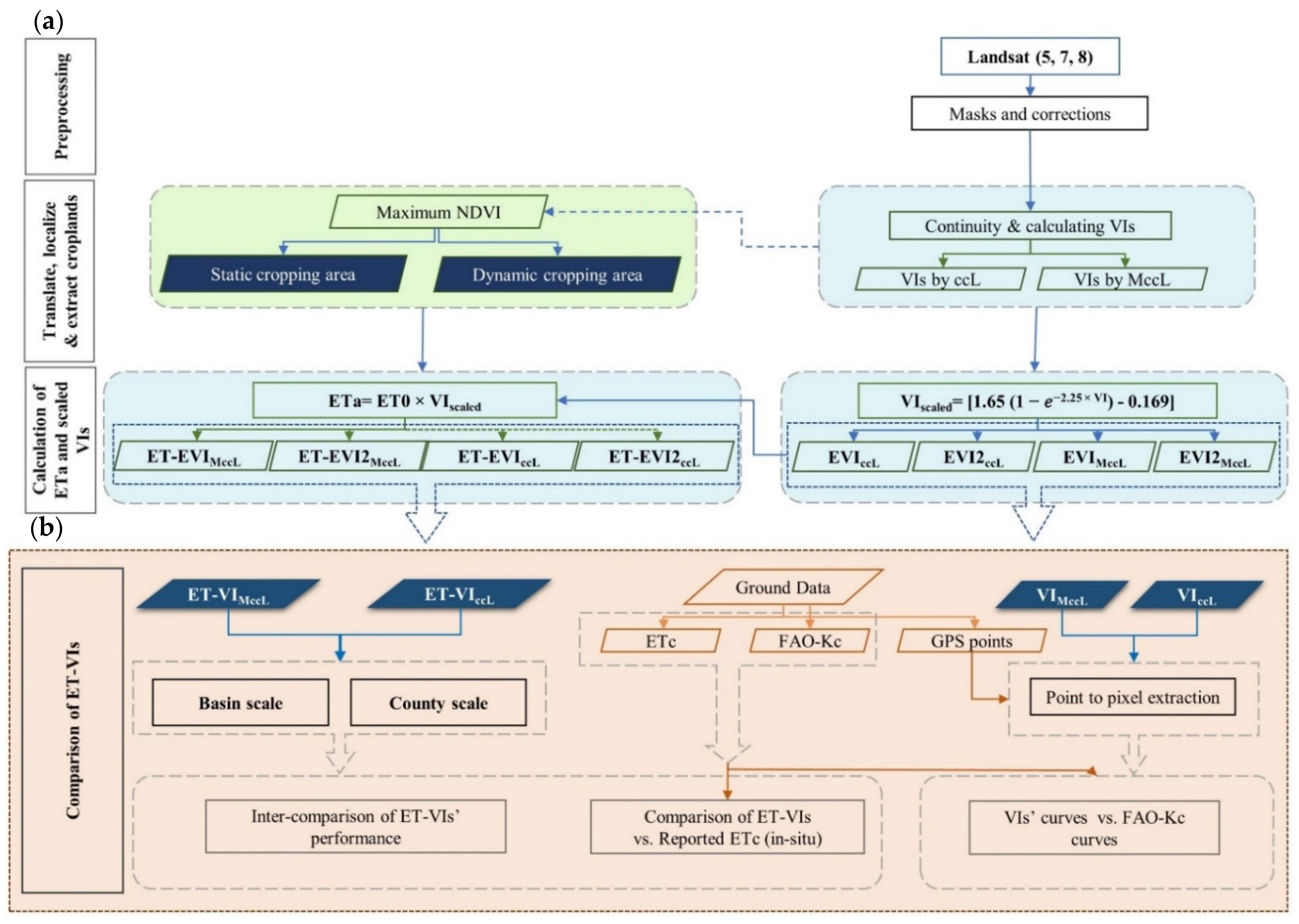
2. Materials and Methods

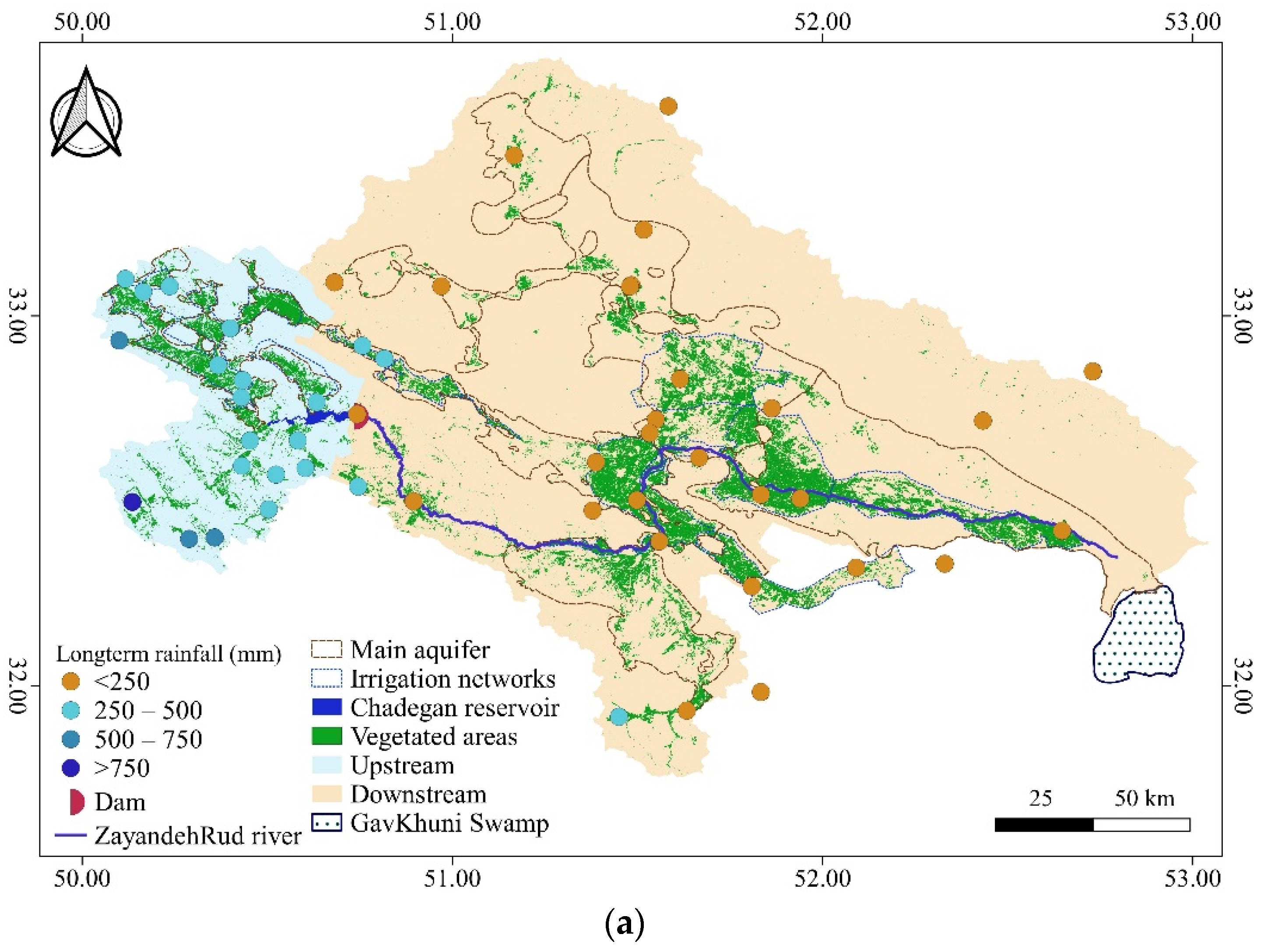
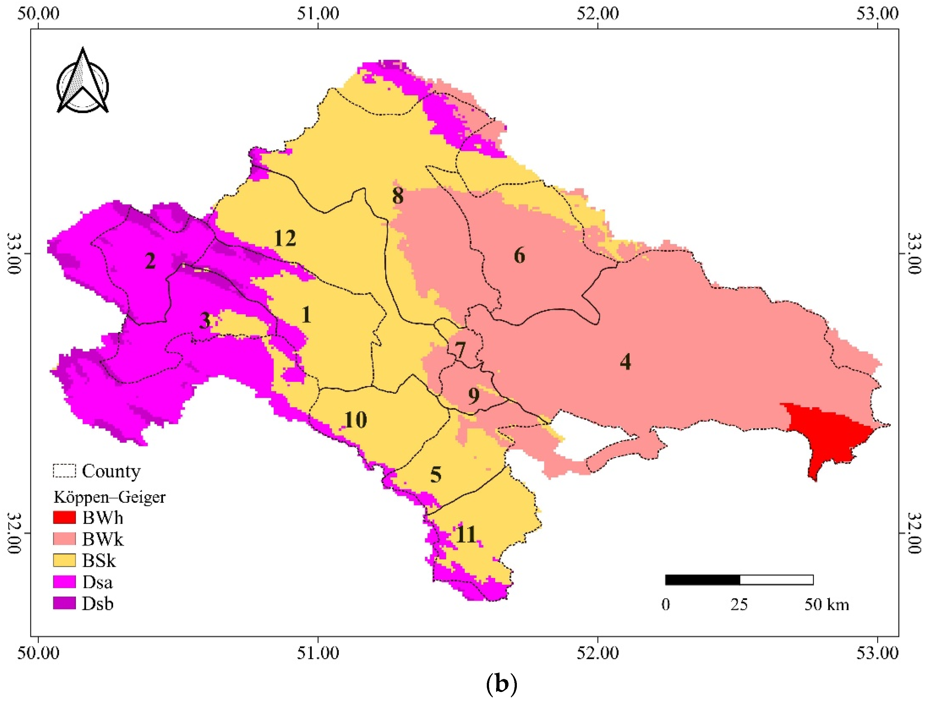
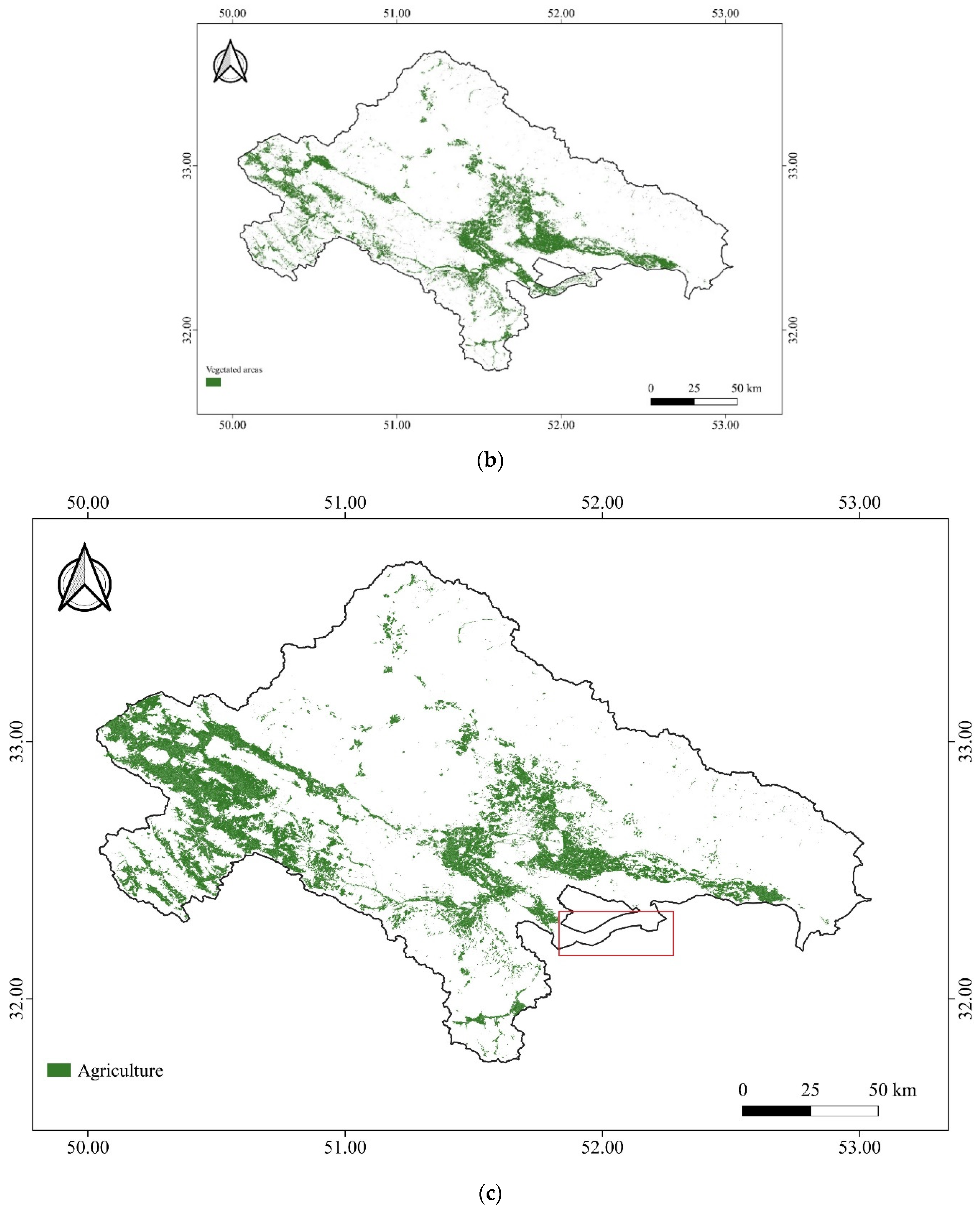
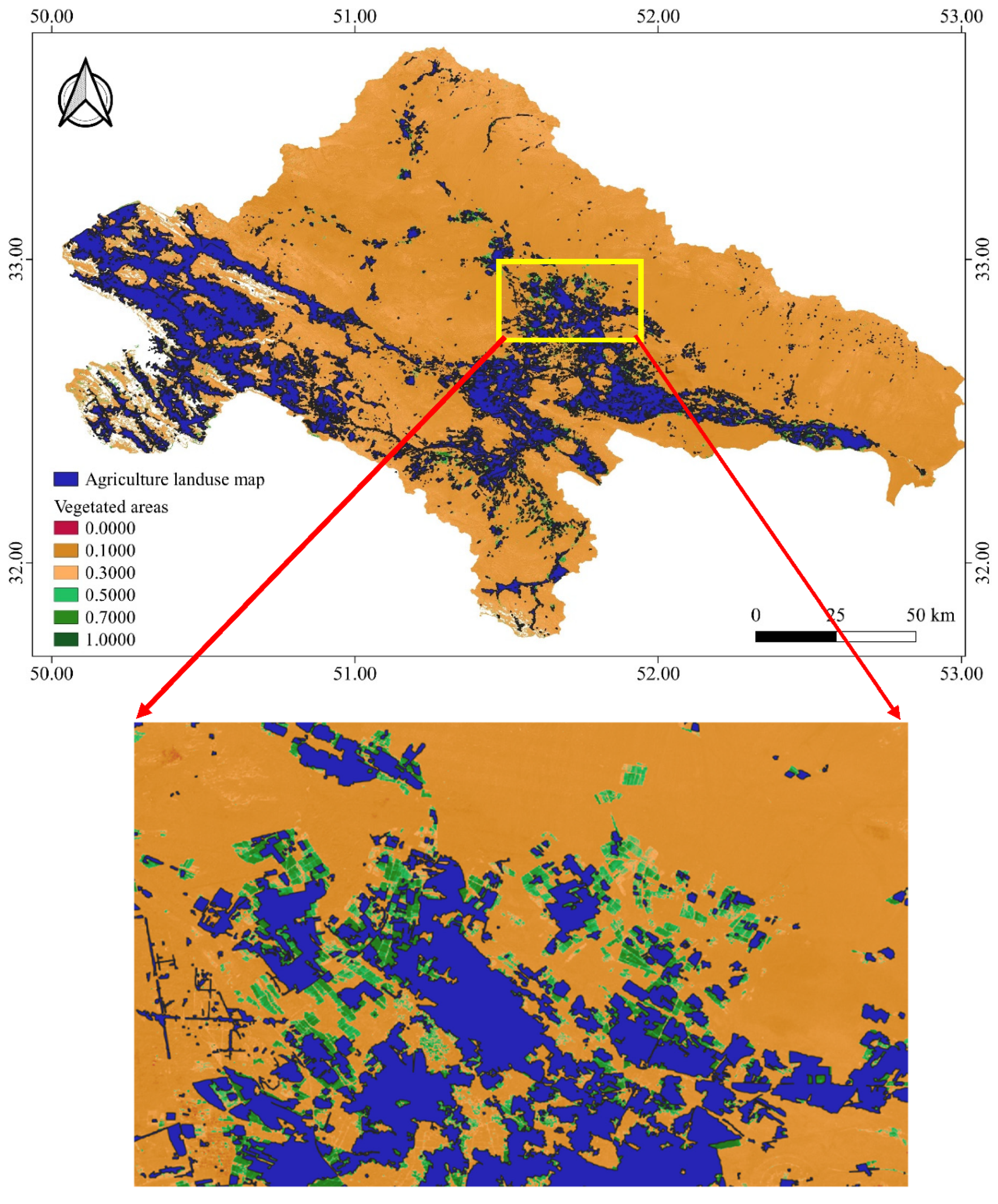
2.1. Study Area

With the second largest population in the Near East and North Africa, 90% of Iran’s agricultural production depends on irrigation. The central, eastern, and southern parts of Iran have experienced drought leading to a challenged agriculture sector [43]. This work looks at a closed river basin, the ZRB, which is located in the arid region of central Iran. Agriculture is the main use of water and consumes about 80% of the water resources [44]. A long-term record of agricultural water use is lacking but is needed because it plays a key role in the water management of this region. Apart from the climatological characteristics of the region, there is a chronic lack of a centrally organized ETa data bank. The need for accurate and spatially explicit ETa data is critical for water management in this region, especially considering climate change and reoccurring droughts.

The ZRB covers an area of 26,917 km² (Figure 1). The main river of the ZRB flows for 350 km from the Zagros Mountains to the Gavkhuni Swamp [45]. The Zayandehrud dam is the main reservoir and plays a key role in regulating the water supply [46]. Precipitation data from 53 stations (2003 to 2018, data were obtained from the Islamic Republic of Iran Meteorological Organization (IRIMO)) demonstrate that the average precipitation varies from 63 mm in the eastern part to 1281 mm in the western part (Figure 1a). Precipitation occurs mainly from November to April. The mean annual temperature is 14.2 °C. The elevation of the study area varies from 1442 m to 3927 m. According to the Isfahan Agricultural Organization (IAO), more than 40 different crops are cultivated in the region, with wheat, barley, alfalfa, maize, potatoes, onions, and rice being the main staple crops. Owing to the low precipitation in the eastern and central parts of the ZRB, irrigated agriculture is dominant. Water paucity, drought, and low rainfall are the main challenges in the ZRB, and these have resulted in fewer water releases from the dam downstream of the ZRB. In this study, downstream refers to the area from the dam to the Gavkhuni swamp, and from the dam upwards, where it rains more frequently, is referred to as upstream. Twelve counties cover about 92% of the basin’s area and are mainly located in arid and semi-arid regions (Figure 1b, Köppen-Geiger climate zones [47]).

2.2. Localization of MODIS-Based EVI(EVI2) and ETa

Different VIs were calculated using images from Landsat 5, 7, and 8 at a spatial resolution of 30 m (Figure S1 displays the spatial footprint of Landsat scenes over the ZRB) and a temporal resolution of 16 days and from MODIS (daily 250 m MOD09GQ and 500 m MOD09GA land surface reflectance products). Landsat images were processed using the Google Earth Engine (GEE) platform (https://earthengine.google.com, accessed on 20 June 2021). GEE is a cloud-based platform for geospatial analysis with massive computational capabilities and direct access to RS data [48]. MOD09GQ and MOD09GA products [49] were acquired to derive the transformation equations for EVI and EVI2 across MODIS and Landsat (Figure 2).

To calculate ETa, ETo was first computed by applying the Global Crop Water Model (GCWM) using the FAO–PM method [50] and hourly ERA5-reanalysis data with 0.25 degrees spatial resolution aggregated to daily climate input. The model was executed in daily time steps with a spatial resolution of 5 arc-minutes (about 8 Km) [51]. Statistical analysis and visualization of the results were conducted in R [52] and QGIS [53].

2.2.1. Preparation and Generation of MODIS-Like Landsat Images VIs

Landsat surface reflectance images (2000–2019) were corrected for topography and bidirectional reflectance distribution function (BRDF). Clouds, shadow, snow, water, and poor-quality pixels were masked out. Landsat 7 missing values due to the Scan Line Corrector error were simply ignored and only available pixels within the scene were used. Problems along the edges of Landsat 5 images which resulted in missing data were also removed by applying an inwards-buffer mask. Furthermore, there were small differences between the spectral characteristics of Landsat 5, 7, and 8 which created a bias [54]. To address the first research question regarding translation and localization of MODIS-based EVI(EVI2) and ET equations, we investigated the differences resulting from the spectral characteristics of Landsat 5, 7, and 8. We did this by comparing two translations approaches and their impacts on ETa:

• Roy et al. [54] developed transformation equations to reduce the effects of these small differences and produce a sensor-independent, long-time series of Landsat composites. These functions, which are also available on the GEE platform, were applied on Landsat images to calculate continuity-corrected Landsat (ccL) VIs and incorporate them into the ETa equation directly to derive ET-VIs (ET-EVI_ccL, and ET-EVI2_ccL).
• The ETa equation applied in this study was originally developed using MODIS images. The second approach to reduce the effects of these differences is to translate VIs derived from Landsat images into MODIS-like VIs. For this purpose, MODIS daily products MOD09GQ (250 m, red (R), near-infrared (NIR)) and MOD09GA (500 m/L km, blue (B), zenith angle (Vz), and Quality Assessment (QA)) were downloaded. MOD09GA was resampled to 250 m to support the generation of a 250 m spatial resolution data set. EVI and EVI2 were computed after applying cloud and aerosol filtering. The resulting Landsat data was resampled to MODIS 250 m. A regression model was then estimated between matching dates to derive four conversion equations: two for calculating MODIS continuity-corrected Landsat (MccL) (EVI_MccL and EVI2_MccL) from Landsat 8, and two for those of Landsat 5 and 7 (data processing was conducted at the Vegetation Index and Phenology laboratory at the University of Arizona (https://vip.arizona.edu/, accessed on 17 February 2021). To characterize these empirical translation methods and their impacts on the derived ETa, we compared pairs of MODIS ET-VIs (ET-EVI_MccL and ET-EVI2_MccL) against non-MODIS-based ET-VIs (ET-EVI_ccL and ET-EVI2_ccL).

2.2.2. Calculation of Vegetation Indices

EVI was developed to address some issues in NDVI, including sensitivity to soil background, saturation over dense canopies, and sensitivity to the residual atmosphere. EVI uses the ratio of NIR, R, and B bands to extract canopy greenness (Equation (1)).

$$\mathrm{EVI}=\mathrm{G}\frac{\mathrm{NIR}-\mathrm{R}}{\mathrm{L}+\mathrm{C}1\mathrm{R}-\mathrm{C}2\mathrm{B}+1}$$

(1)

where G is a gain factor, C1, C2 are the coefficients of the aerosol resistance, which uses the B band to correct for aerosol effects in the R band, and L functions as the soil adjustment factor. The values adopted for MODIS are L = 1, C1 = 6, C2 = 7.5, and G = 2.5 [55].

EVI is quite sensitive to variations in the B band reflectance and is useless in sensors without a blue band, which hampers its consistency across different sensors. EVI2 was introduced to address these challenges and requires only NIR and R bands (Equation (2)) [56]. EVI2 may become slightly susceptible to aerosols due to omitting the B band. However, modern RS data applies very strict quality assurance to assist with poor-quality data removal. The differences between EVI and EVI2 were reported to be roughly ±0.02 [31,56].

$$\mathrm{EVI}2=2.5\frac{\mathrm{NIR}-\mathrm{R}}{\mathrm{NIR}+2.4\times \mathrm{R}+1}$$

(2)

The following translation and conversion equations were applied to the VIs time series to generate ET-EVI_MccL and ET-EVI2_MccL:

EVI_MccL (Landsat 8) = 0.848368 × EVI (Landsat 8) + 0.02552

(3)

EVI2_MccL (Landsat 8) = 0.848368 × EVI2 (Landsat 8) + 0.02649

(4)

EVI_MccL (Landsat 5 and 7) = 0.842328 × EVI (Landsat 5 and 7) + 0.0240124

(5)

EVI2_MccL (Landsat 5 and 7) = 0.8990118 × EVI2 (Landsat 5 and 7) + 0.0234406

(6)

To understand how these empirical translation methods applied to Landsat VIs impact the resulting ETa estimation, VIs were compared before and after applying MODIS-based equations. Two Landsat scenes (14 June 2002 and 1 August 2008) during the growing season were selected with maximum coverage of the basin and the least cloud contamination. To demonstrate the differences between the VIs over the scene, four combinations of pixel-wise differences were applied between EVI_ccL and EVI2_ccL, EVI_MccL and EVI2_MccL, EVI_MccL and EVI_ccL, and EVI2_MccL and EVI2_ccL.

2.2.3. Calculation of ETa

Nagler et al. [24] developed a MODIS-based ETa algorithm using the Beer–Lambert Law to express canopy light absorption and EVI replacing leaf area index (LAI). This method was applied over riparian and agricultural areas in the southwestern U.S. and later adapted to Landsat in urban green spaces [5], riparian zones [39], and, in this study, for the first time, ET-VIs were developed for croplands at 30 m resolution (considering harvested areas’ changes) at the basin scale using GEE. The ETa equation:

$$\mathrm{ETa}\left(\mathrm{mm}\right)=\mathrm{ETo}\left(\mathrm{mm}\right)\times \left[1.65\left(1-{\mathrm{e}}^{-2.25\times \mathrm{VI}}\right)-0.169\right]$$

(7)

where (1 − e^[−b×VI]) is derived from the Beer–Lambert Law to estimate light absorption by a canopy. Using this ETa equation, four ETa products (ET-EVI_MccL, ET-EVI2_MccL, ET-EVI_ccL, and ET-EVI2_ccL) were calculated for all available Landsat images over the study area at an annual scale.

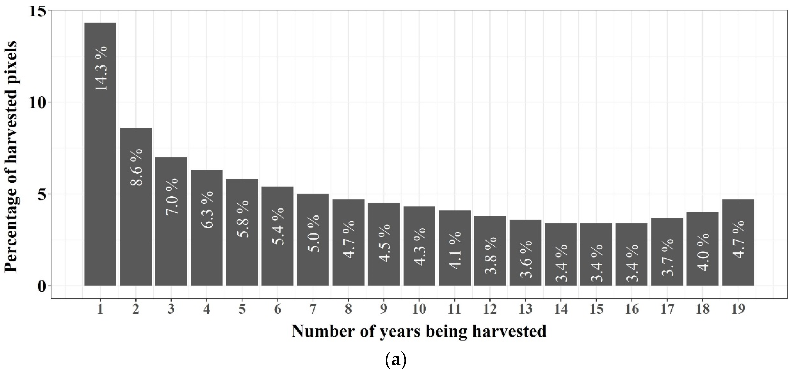
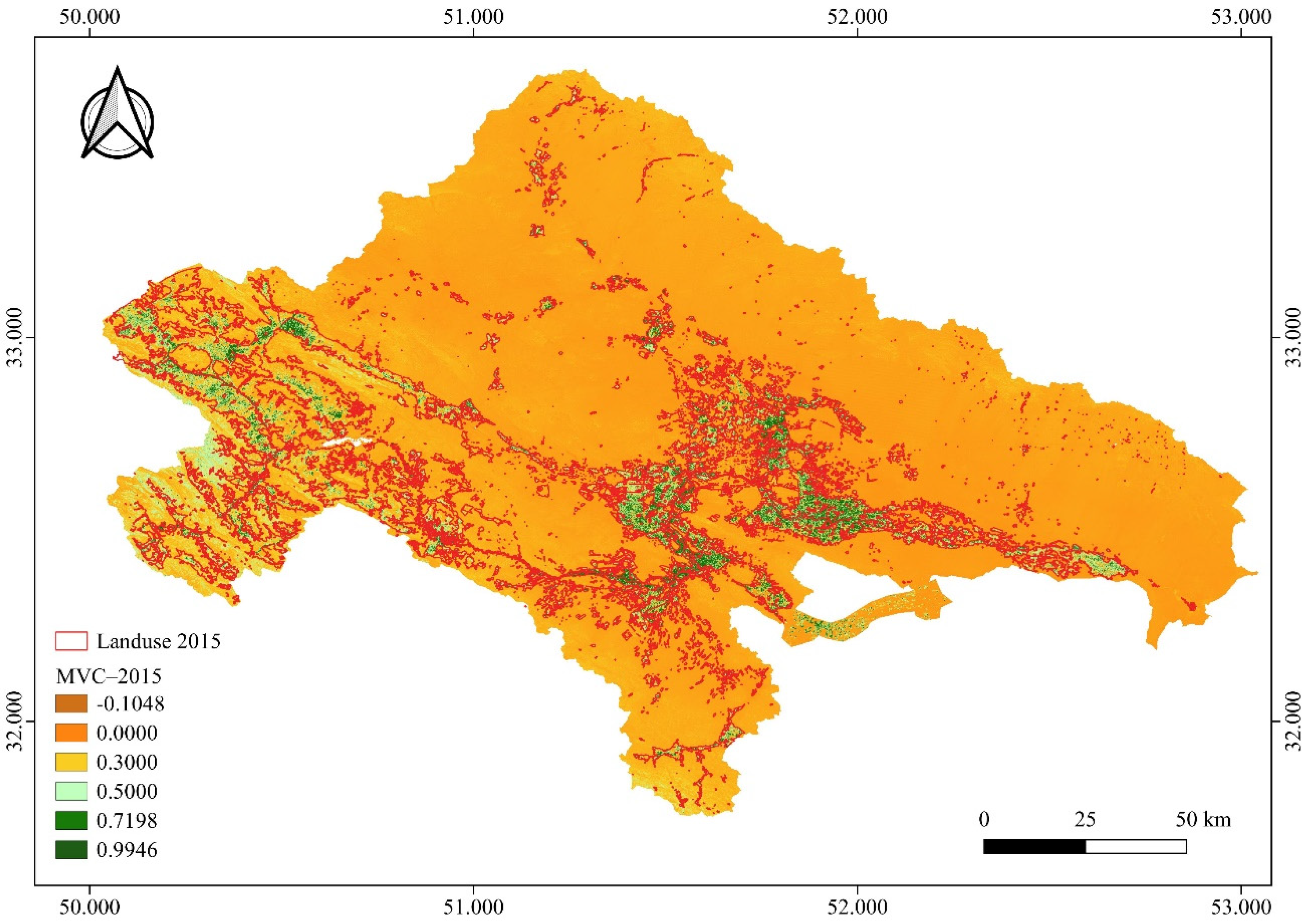
2.3. Crop Cover Dynamics

To assess the difference in ETa caused by considering a static or dynamic cropping area, annual maximum NDVI layers were derived from Landsat images for two decades using GEE. The annual maximum NDVI layers were developed by applying the maximum value composite (MVC) method, which generates a composite image over a given period by preserving for each pixel the maximum NDVI value of images. Maxwell et al. [57] used variable thresholds ranging 0.61 to 0.71 for MVC to detect ever-cropped lands over the 27 years in southwestern Kansas at county-level [57]. To exclude all but cropped lands from MVC, we excluded all NDVI values using three empirical thresholds less than 0.4, 0.5, and 0.6. After visual inspection and spatial analysis of all MVC layers and comparing croplands and non-cropland areas using Google Earth maps, we found out that by removing values less than 0.4 some rangelands remained in the cropland MVC layers, and by using 0.6 some cropping areas were excluded; therefore, 0.5 was used to minimize rangelands and other covers.

Pixels with high NDVI are agricultural areas. Good and medium rangelands located upstream mostly had NDVI values of about 0.5. We also used a land use map prepared by the Ministry of Energy of Iran (https://moe.gov.ir/?lang=en-US, accessed on 20 February 2021) to evaluate our cropland layers. It depicts fallow land, orchards, rainfed cropland, spring, and fall irrigated agricultural areas. This land use map was produced (2015) using an interpretation of Landsat 8 images. Visualizing and overlaying the land use map on the Google Earth and MVC maps showed that not all green spaces and trees could be masked out, but the extent of this vegetation was insignificant compared to the croplands. After the preparation of MVC, annual cropland layers were then used to derive the ETa over the study period. To examine the impact of cropping areas’ changes on ETa, we also extracted a static cropping area for the whole study period using MVC to identify land that was cropped at least once during the study period (ever-cropped land) using the time series of Landsat satellite imagery. The static layer was used to calculate ETa and was then compared against ETa derived by considering annual changes of cropping area (i.e., dynamic cropping area).

2.4. Comparison of Landsat VIs and ETa with Ground Data

To compare VIs and ET-VIs with in-situ data, estimated ET-VIs were compared to long-term average ETc values reported by the Isfahan Agricultural and Natural Resources Research and Educational Center (IANREC) at the county scale for major crops. IANREC has used the dual crop coefficient approach (Kc = Kcb + Ke) to calculate ETc. The basal crop (Kcb) and Ks values reported by FAO56 were adjusted based on the methodology proposed by [35] using ground data, i.e., minimum relative humidity, wind speed, and the average plant height for the year 2013. The soil evaporation coefficient (Ke) was calculated considering soil physical properties, irrigation intervals, and irrigation depth. Kcb and Ke were combined with ETo values to calculate ETc (ETc = (Kcb + Ke) × ETo). The ETc values obtained from IANREC were only reported as an average value for each crop and the whole study period. To detect the major crops in each county, annual statistics for crop type, production, and cultivated area were acquired (https://agri-es.ir/Default.aspx?tabid=1925 accessed on 1 June 2021). Wheat and barley observations were obtained for the growing season 2018–2019 from IAO in order to evaluate RS-VIs against typical curves of Kc values used by FAO. To compare the VIs, monthly VIs were extracted (Equation (8)):

VI_scaled = [1.65 (1 − e^{−2.25×EVI (or EVI2)}) − 0.169]

(8)

Four scaled VIs (EVI_MccL, EVI2_MccL, EVI_ccL, and EVI2_ccL) were calculated and compared with FAO-Kc curves. Control points of two crops (wheat and barley) in Isfahan County, collected over February–March 2019, were used to determine if the estimated scaled VIs represent reported ones. Kc and VIs are sensitive to LAI and fractional ground cover (reviewed in [37,38,58]). Their minimum occurs at the early stages of crop cultivation (initial (ini)), changes with crop development, reaches the maximum at grain filling (mid-season (mid)), and decreases at the end season (end) [59]. A point-to-pixel method was applied to extract the corresponding pixel values at each point. Considering the crop calendar of wheat and barley (November–June), scaled VIs were compared to those of FAO56.

To assess the performance of scaled VIs against reported FAO-Kc values for wheat and barley, the RMSE was applied at three quartiles (25, 50, and 75). Also, reported long-term average ETc values of major crops in each county were compared with the long-term average of ET-VIs estimates within the counties. ETc was calculated under no-stress conditions. Local ETc values are the only available ground data at the county level for the ZRB; therefore, they were used as a proxy for ET-VIs’ performance evaluation.

2.5. Performance Analysis of ET-VIs

ET-VIs were compared using annual average values, minimum and a maximum of annual ET-VIs, visualization of annual ET-VIs, and ETa anomaly at basin level. In addition, the pixel-wise spatial correlation was calculated between:

• ET-EVI_ccL and ET-EVI2_ccL;
• ET-EVI_MccL and ET-EVI2_MccL;
• ET-EVI_ccL and ET-EVI_MccL;
• ET-EVI2_ccL and ET-EVI2_MccL.

The correlation coefficient (R²) at the pixel level was calculated and used to compare the differences between ET-VIs. The Mann–Kendall (MK) test was applied to detect the existence of trends in ETa estimations in each county. MK is a non-parametric test used to identify monotonic trends present in time series. The null hypothesis considers no trend among the observations and the alternative hypothesis represents a monotonic trend [60]. Since the MK test cannot provide the slope of the trend (magnitude), the Sen method, a nonparametric estimator [61], was used to determine the magnitude of the trend [62]. Negative S values show a downward trend and positive values present an upward trend.

3. Results

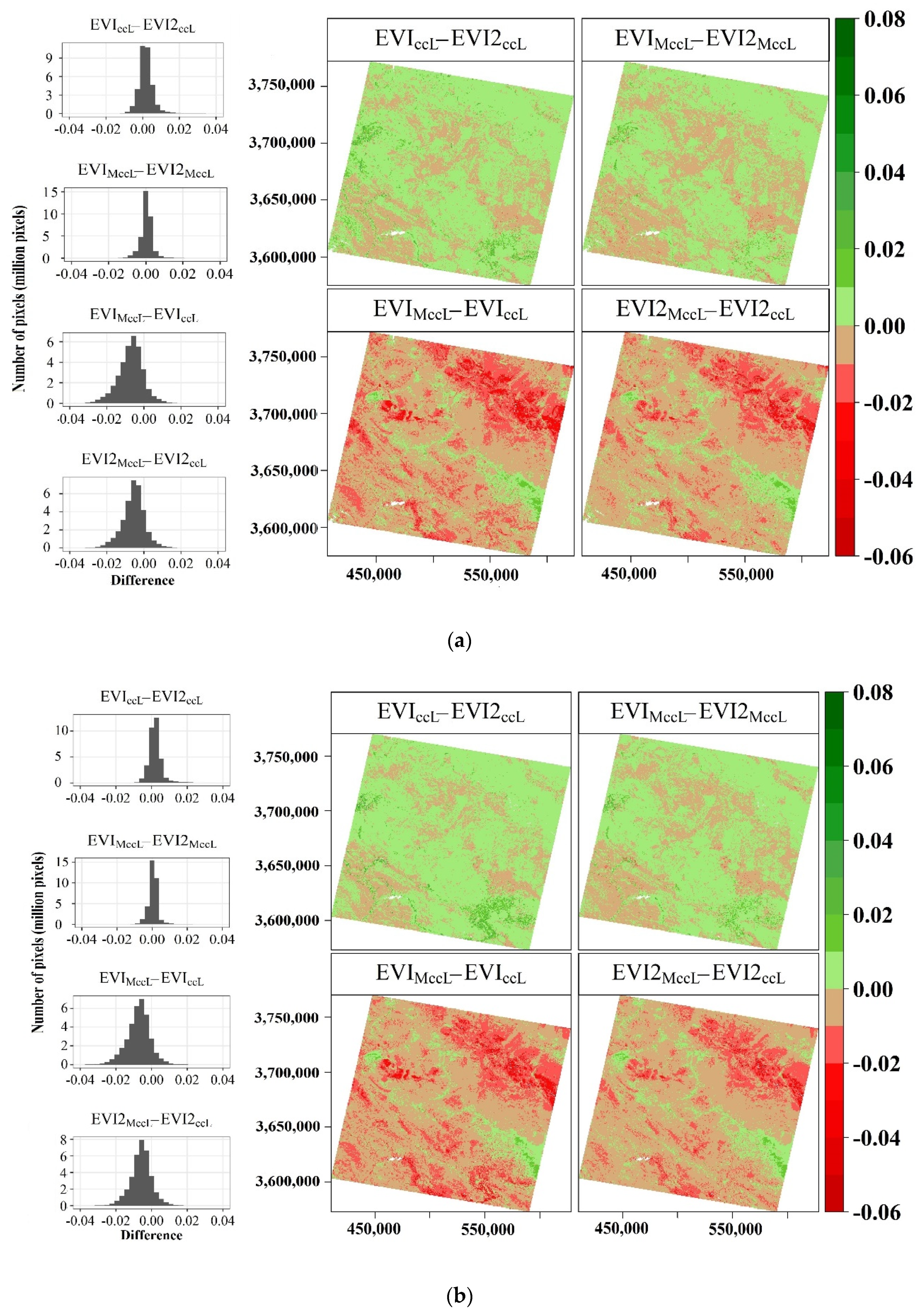
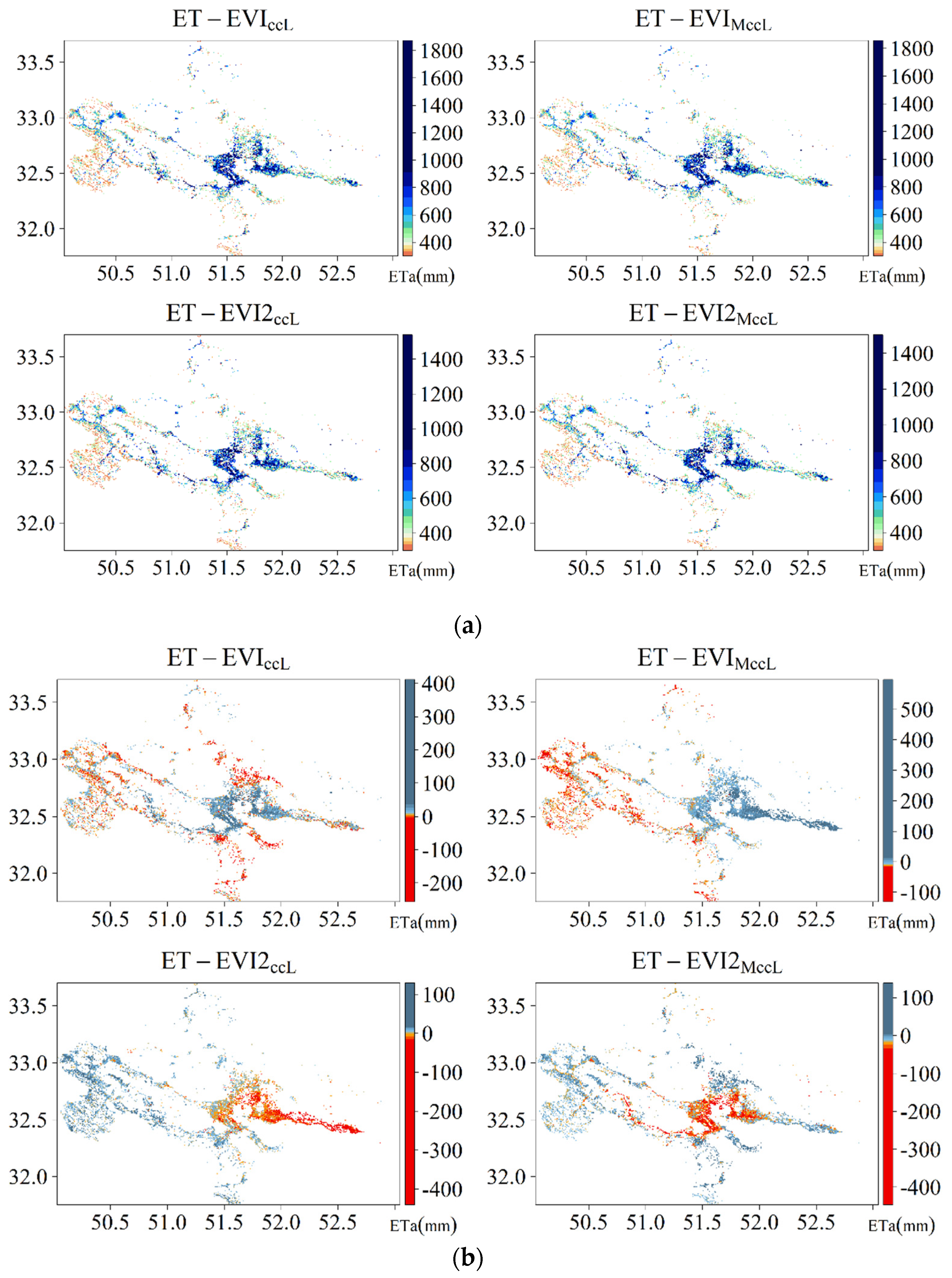
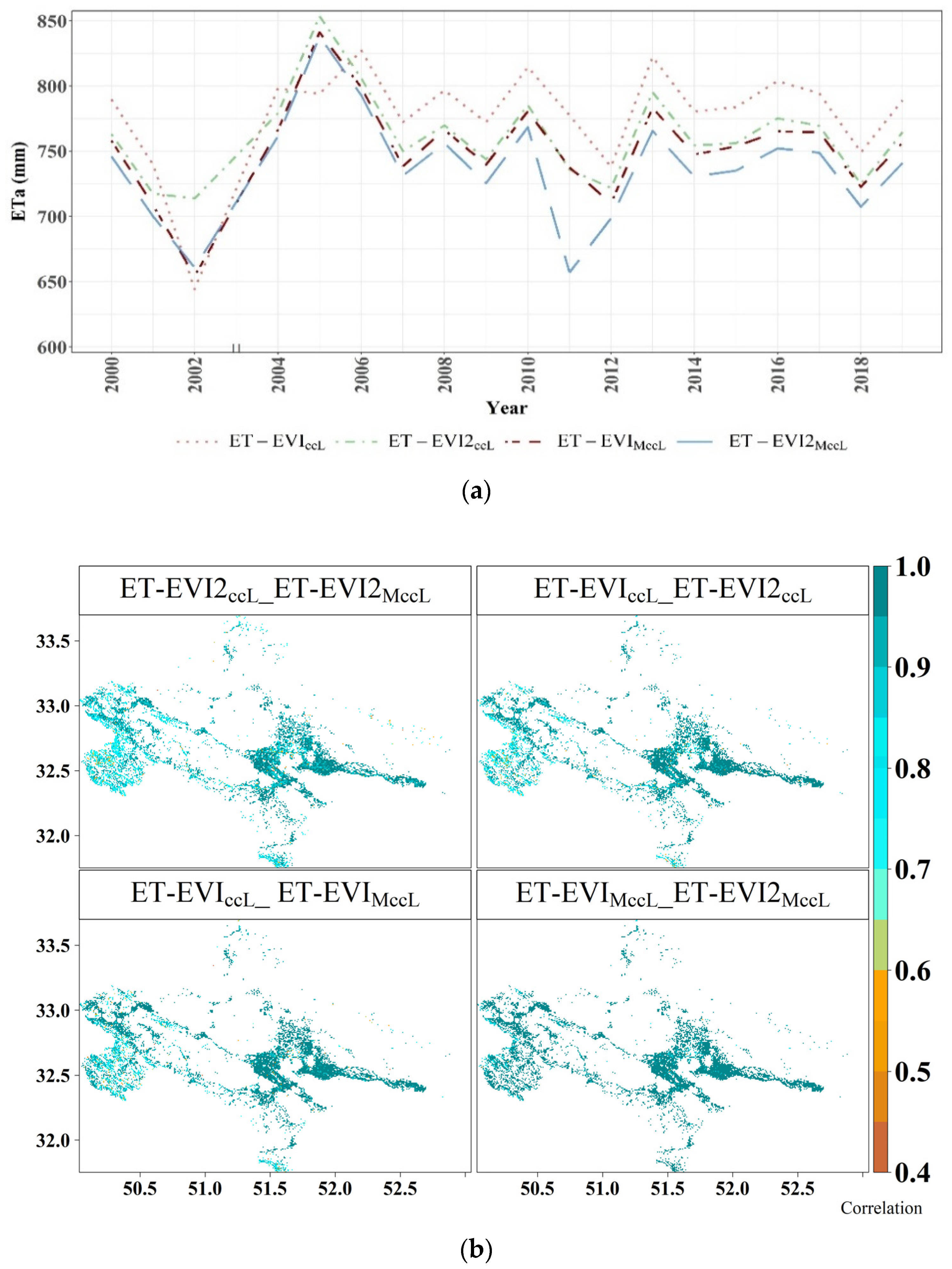
3.1. Localization of MODIS-Based EVI(EVI2)

Calculated VIs were compared on two dates, 14 June 2002 and 1 August 2008, in four combinations (EVI_ccL–EVI2_ccL, EVI_MccL–EVI2_MccL, EVI_MccL–EVI_ccL, and EVI2_MccL–EVI2_ccL). Both difference maps and difference frequency histograms of EVI_ccL and EVI_MccL were higher over dense vegetation (Figure 3). ET-EVI2_ccL and EVI2_MccL presented slightly lower values than corresponding EVI values, particularly over bare soil and mountainous regions. The highest and lowest estimated values belonged to EVI_ccL and EVI2_MccL, respectively, as evidenced by histograms. The peak of the EVI_MccL–EVI_ccL and EVI2_MccL–EVI2_ccL histograms shifted to more negative values compared to that of the EVI_ccL–EVI2_ccL and EVI_MccL–EVI2_MccL. In some parts of sparsely vegetated areas, the EVI2_MccL and EVI2_ccL values were slightly larger than EVI values. While these differences are still well within the expected noise in the VI dynamic range, [31] explained that EVI2 values are somewhat higher than EVI values due to the higher ratio of B/R in the EVI equation.

3.2. Impacts of the Static and Dynamic Cropping Areas on ETa Estimation

Static cropping areas resulted in the considerable underestimation of mean ETa (mm) and the overestimation of the total ET (km³) due to the consideration of non-cultivated areas in ETa derivation over the years (Figure 4). Furthermore, inappropriate NDVI threshold results in over- or underestimation. By removing values of less than 0.4, some rangelands remained in the MVC layers, and by using 0.6 some cropped lands were excluded; therefore, 0.5 was used to exclude rangelands from croplands.

The average difference in mean ET between ET estimated based on static versus dynamic cropping area ranges from 221.7 mm (ET-EVI2_MccL) to 239.7 mm (ET-EVI_ccL). When comparing the volume of ETa in km³ with regard to static cropland, we underestimated the ETa intensity in mm but we overestimated total ETa in km³ since the area of static cropland is larger than that of dynamic areas (Figure 4b). To find out to what extent our method in cropland detection is reliable, we compared our static cropland layer and MVC of 2015 with the available land use map (Appendix A, Figure A1, Figure A2 and Figure A3). This land use map was generated in 2015 and does not capture recent changes in agricultural areas. About 60 percent of our static layer covered the agriculture land use map. This is due to the fact that the static layer considers changes in croplands for the whole period (i.e., 2000 to 2019), while the land use map reflects the changes that have happened within a few years up to 2015. The main discrepancy between the static layer and land use map was over rainfed areas in the upstream area. Moreover, the MVC of 2015, as expected, showed lower cultivated areas compared to the agriculture land use map. The reason is that the MVC of 2015 presented only cultivated areas of a given year i.e., 2015.

3.3. Comparing Scaled VIs and ETa with Reported Values

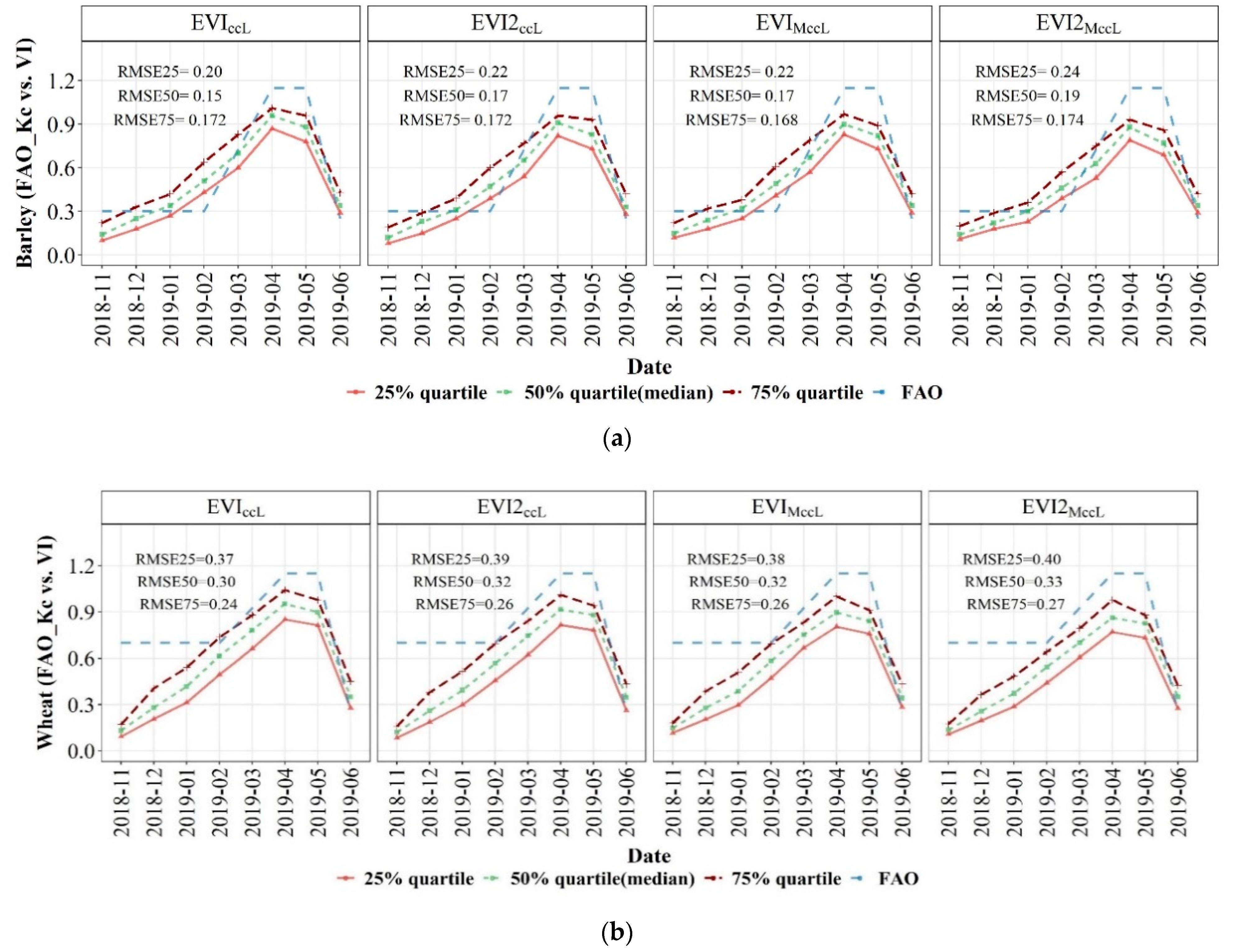
3.3.1. Evaluation of Scaled VIs with FAO-Kc

Kc methods are typically derived from crops grown under optimal conditions, whereas actual field crops can be subjected to various limitations and water stress [24,63]. The monthly average of scaled VIs curves versus FAO-Kc at three quartiles for wheat and barley have relatively close RMSE values (Figure 5).

EVI_ccL has the lowest RMSE values at almost all growth stages compared to other VIs while the highest RMSE belongs to EVI2_MccL. The curves of scaled VIs estimates were almost similar to that of FAO-Kc. The initial stages in the VI- and FAO-based Kc curves have considerable differences for wheat. Scaled VIs for wheat have larger RMSE rates at all growth stages, particularly at initial and mid-season stages. All scaled VIs’ RMSE rates decrease when approaching the end-season. The reason can be the evaporation after irrigation or rainfall and sensitivity of reflectance to the soil top-layer wetness, whereas at the end of the season soil evaporation is diminished. The VI method considers transpiration from green vegetation, and only a small extent of evaporation from bare soil; therefore, underestimations happen during the initial and developing stages of the crop cycle.

3.3.2. Evaluation of ET-VIs with ETc

To assess the ET-VIs’ estimates, long-term average ETa estimates were compared with that of reported ETc values (

Table 1. Long-term average ET-VI and reported ETc, county: 1: Tiran, 2: Freydan, 3: Chadegan, 4: Isfahan, 5: Mobarakeh, 6: Borkhar, 7: Khomeinishahr, 8: Shahinshahr, 9: Falavarjan, 10: Lenjan, 11: Dehaghan, 12: NajafAbad. ET-EVI2_MccL and ET-EVI_MccL: ET calculated using 2- and 3-band Enhanced Vegetation Index (MODIS continuity-corrected Landsat) respectively; ET-EVI2_ccL and ET-EVI_ccL: ET calculated using 2- and 3-band Enhanced Vegetation Index (continuity-corrected Landsat) respectively.

	Long-Term Average ETa				Reported	Percentage of ETa Difference from ETc
County	ET-EVIccL	ET-EVI2ccL	ET-EVIMccL	ET-EVI2MccL	ETc	ET-EVIccL	ET-EVI2ccL	ET-EVIMccL	ET-EVI2MccL
1	778	772	752	745	602	29	28	25	24
2	645	646	621	621	565	14	14	10	10
3	656	657	632	632	568	15	16	11	11
4	845	812	824	794	774	9	5	6	2
5	792	779	763	751	705	12	11	8	6
6	678	680	673	673	632	7	8	7	7
7	979	945	937	907	732	34	29	28	24
8	666	672	653	658	607	10	11	8	8
9	914	877	877	842	733	25	20	20	15
10	861	837	816	795	691	25	21	18	15
11	672	685	658	670	570	18	20	15	17
12	876	856	844	826	724	21	18	17	14
Basin	778	762	752	738	643	21	19	17	15

). The results show that all ET-VIs exceeded ETc values. Among ET-VIs, ET-VI_MccL and particularly ET-EVI2_MccL, showed lower values than those of others. The maximum differences between ET-VIs and ETc for all ET-VIs occurred in Khomeinishahr (Figure 1), ranging from 34% (ET-EVI_ccL) to 24% (ET-EVI2_MccL). The correlation between ET-VIs and ETc values at the county scale ranges from 72% (ET-EVI2_ccL) to 78% (ET-EVI_MccL).

To find out how much NDVI thresholds can affect resulting ET-VIs, ET-VIs were calculated at three thresholds of 0.4, 0.5, and 0.6 (see Section 2.3).

Table 2. Long-term average ET-VI and reported ETc considering different NDVI thresholds. ET-EVI2_MccL and ET-EVI_MccL: ET calculated using 2- and 3-band Enhanced Vegetation Index (MODIS continuity-corrected Landsat) respectively; ET-EVI2_ccL and ET-EVI_ccL: ET calculated using 2- and 3-band Enhanced Vegetation Index (continuity-corrected Landsat) respectively.

	Long-Term Average ETa				Reported	Percentage of ETa Difference from ETc
NDVI Threshold	ET-EVIccL	ET-EVI2ccL	ET-EVIMccL	ET-EVI2MccL	ETc	ET-EVIccL	ET-EVI2ccL	ET-EVIMccL	ET-EVI2MccL
MVC_0.4	715	700	691	678	643	11	9	7	6
MVC_0.5	778	762	752	738	643	21	19	17	15
MVC_0.6	835	818	808	792	643	30	27	26	23

presents estimated ET-VIs considering three different MVC thresholds to extract croplands over time. As can be seen, ET-EVI2_MccL and ET-EVI_MccL have smaller differences at all MVC thresholds when compared with ETc values.

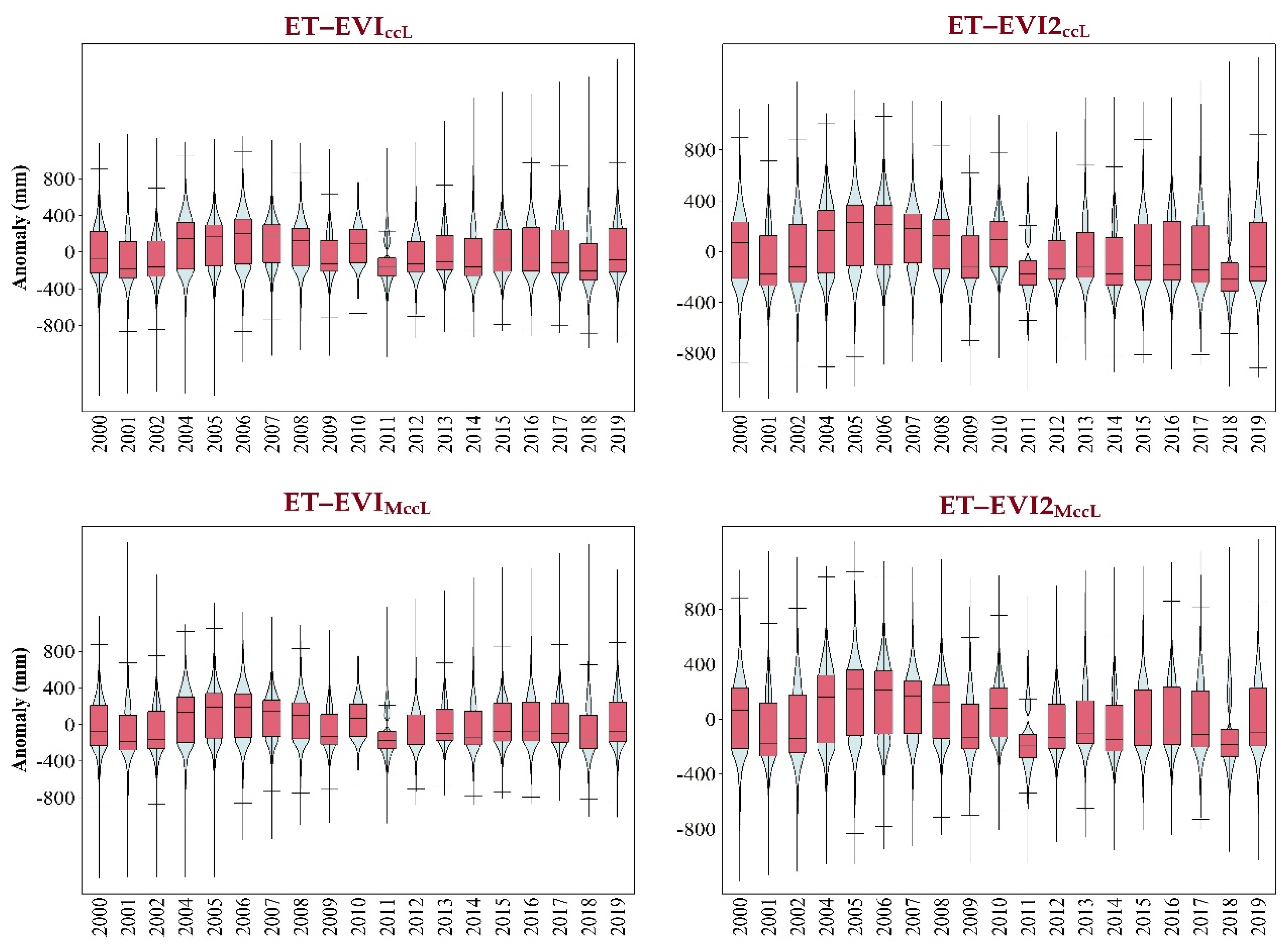
3.4. Performance Analysis of ET-VIs

To compare the performance of the ET-VIs over the ZRB, annual and long-term averages of ET-VIs were provided (Figure 6). Since the differences between ET-VIs, owing to the small area of cultivation and close changes of ET-VIs, are not visible in the maps, we subtracted ET-VIs from the average of all ET-VIs presented in Figure 6a in order to better visualize the changes of the ETa estimates (Figure 6b). Our results (Figures S2–S5) demonstrated that all the ET-VIs have lower ETa in the northwestern part of the ZRB and higher ETa all along the river. Nearly all annual ET-VIs showed that the highest ETa estimates were recorded from 2004 to 2007 when rainfall was adequate and also much more water was released from the dam to the lower reaches of the ZRB. All ET-VIs except ET-EVI2_MccL recorded the lowest ETa values over the ZRB in 2002 and 2012. ET-EVI2_MccL recorded the lowest ETa rates over the basin in 2002 and 2011. Also, maximum ET-VIs rates were observed in 2005 over croplands in the ZRB. The lowest minimum values belong to ET-EVI_MccL and ET-EVI2_MccL (Table S1). By contrast, ET-EVI_ccL and ET-EVI2_ccL have the highest maximum and average numbers in most of the counties (Figure 6b).

Cultivation density should be considered when comparing irrigated and rainfed regions, as irrigated crops mostly have a higher vegetation density. To show the performance of the ET-VIs over croplands, we selected two counties (Figures S6 and S7): one with the highest rainfed area in upstream (Chadegan) and one with the highest ETa values in the ZRB (Khomeinishar). The ETa decreases with the distance from the river, reflecting reduced access to water.

Performance of the ET-VIs over Chadegan: with a cropping area of 34,000 ha and a 357 mm average precipitation, Chadegan has rainfed areas with no access to surface and groundwater. With no supplementary irrigation, precipitation is expected to be higher than ETa. In this county, ET-EVI_MccL and ET-EVI2_MccL estimates were lower than those of ET-EVI_ccL and ET-EVI2_ccL. Although the amount of estimated ETa for all VIs was higher over irrigated areas than rainfed areas, the ET-VIs exceeded precipitation in rainfed croplands. The average lowest and highest difference values belong to ET-EVI_MccL (135 mm) and ET-EVI2_ccL (156 mm) respectively.

Performance of the ET-VIs over Khomeinishar: with a cropping area of 5000 ha and a 117 mm average precipitation, Khomeinishar is the smallest county located in the arid part of the ZRB. Two high consumptive crops, pear, and rice, might be the reason for high ETa estimates (907–979 mm) over this region. ET-EVI_ccL resulted in the highest ETa while ET-EVI2_MccL was lower.

A pixel-wise correlation was applied to present the differences between the ET-VIs across the ZRB. Annual graphs of ET-VIs are also depicted in Figure 7 to appraise the ET-VIs’ curves. Figure 7 shows that ET-EVI_MccL and ET-EVI2_MccL perfectly match each other except in 2011. Although ET-EVI_ccL often estimated ETa higher than that of ET-EVI2_ccL, ET-VI_ccL constantly tended to be higher than ET-VI_MccL. Figure 7b shows that both ET-VI_ccL and ET-VI_MccL are strongly correlated at more than 80% over cultivated areas especially alongside the river and in irrigated areas. The lowest agreement between ET-EVIs and between ET-EVI2s are observed across areas with lower vegetation cover; that is, lower correlation and large scattering between the two ETa products (i.e., ET-VI_ccL and ET-VI_MccL). As explained by Nagler et al. [24], the applied algorithm was developed for monitoring dryland irrigation districts and riparian areas and cannot be applied to other landcover types without accounting for that in the empirical derivation.

Figure 8 depicts the boxplots of ET-VIs’ anomalies over two decades. All ET-VIs showed similar patterns considering inter-annual variations in ET-VIs anomalies with a capability to capture the drought and shrinkage of agricultural areas.

ETa has a sharp increase in normal to wet years due to sufficient precipitation and enough available water. From 2000 to 2002, due to drought events [64], negative ET-VIs anomalies persisted throughout the basin, particularly in rainfed areas (Figures S8–S11). In recent years, most rainfed areas have been supplemented with water in the event of water shortage; therefore, the drought impacts and water shortage are not significant upstream compared to downstream. All ET-VIs showed a considerable positive ETa anomaly across the basin from 2004 to 2007 associating with sufficient rainfall and water availability (Figure 8). In 2008, a drought event occurred in the basin, particularly upstream where the river originates, and consequently a significant reduction in ET-VIs is apparent. Similarly, in 2010 and 2017, the amount of precipitation was low and in subsequent years, i.e., 2011 and 2018, a considerable shrinkage in the croplands was conspicuous. It should be noted that the negative ETa anomalies do not correspond to precipitation reduction over the annual scale. Since the rainfall deficit means meteorological drought, any drop of ETa indicates agricultural drought i.e., a decrease in soil moisture. Nevertheless, years with persistent or severe meteorological drought result in negative ETa anomalies. To illustrate the existence and magnitude of trends in ET-VIs at basin and county levels, a summary of trend analysis is presented in

Table 3. The trend in different counties. The critical Z value at the 5% confidence level is ±1.96, and there is a trend if the MK’s Z value is greater than the Z critical value. Also, if the p-value is less than the significance level, the null hypothesis is rejected, meaning that there is a trend in the time series [60]. 1: Tiran, 2: Freydan, 3: Chadegan, 4: Isfahan, 5: Mobarakeh, 6: Borkhar, 7: Khomeinishahr, 8: Shahinshahr, 9: Falavarjan, 10: Lenjan, 11: Dehaghan, 12: NajafAbad. ET-EVI2_MccL and ET-EVI_MccL: ET calculated using 2- and 3-band Enhanced Vegetation Index (MODIS continuity corrected Landsat) respectively; ET-EVI2_ccL and ET-EVI_ccL: ET calculated using 2- and 3-band Enhanced Vegetation Index (continuity-corrected Landsat) respectively.

	ET-EVIMccL			ET-EVI2MccL			ET-EVIccL			ET-EVI2ccL
County	Z	S	P	Z	S	P	Z	S	P	Z	S	P
1	0.56	0.60	0.58	−0.07	−0.20	0.94	1.33	1.40	0.18	0.91	0.75	0.36
2	0.63	2.28	0.53	0.84	1.93	0.40	1.33	3.47	0.18	0.42	0.66	0.67
3	0.91	1.05	0.36	0.63	0.65	0.53	1.47	1.36	0.14	0.84	0.73	0.40
4	−0.98	−1.33	0.33	−1.47	−2.22	0.14	−0.28	−0.34	0.78	−1.12	−1.75	0.26
5	2.24	5.75	0.03	1.47	3.85	0.14	2.73	5.84	0.01	1.61	3.89	0.11
6	3.64	7.90	0.00	3.29	6.76	0.00	3.71	8.79	0.00	3.64	7.74	0.00
7	−0.07	−0.07	0.94	−1.47	−1.92	0.14	0.84	0.95	0.40	−1.05	−1.48	0.29
8	1.75	2.31	0.08	0.70	1.26	0.48	2.17	3.22	0.03	0.70	1.32	0.48
9	1.75	3.74	0.08	1.47	2.40	0.14	2.31	4.58	0.02	1.40	2.52	0.16
10	−0.14	−0.61	0.89	−0.56	−1.07	0.58	0.00	−0.16	1.00	−0.28	−1.02	0.78
11	2.03	3.91	0.04	1.33	3.51	0.18	2.38	4.99	0.02	1.26	3.21	0.21
12	−0.84	−1.40	0.40	−1.33	−2.46	0.18	−0.49	−1.08	0.62	−1.47	−2.19	0.14
Basin	−0.07	−0.08	0.94	−0.35	−0.77	0.73	0.35	0.89	0.73	0.00	−0.03	1.00

. ET-EVI2_MccL in 10 counties had the lowest S values. As mentioned earlier, ET-EVI2_MccL tends to estimate ETa to a lesser degree than those of other ET-VIs. All products presented a downward nonsignificant trend in Isfahan, Lenjan, and NajafAbad. This can be due to less water availability and consequently less soil moisture in the root zone. At the ZRB scale, it was found that the annual ET-VIs, except ET-EVI_ccL, decreased. ET-EVI_ccL presented an upward trend with 0.89 mm/year, which was not statistically significant. A maximum nonsignificant upward trend based upon S belongs to Freydan with 3.47 mm/year. NajafAbad has the highest nonsignificant decreasing trend with 2.46 mm/year. Lenjan is the main rice producer and, due to water shortages, the cultivation of rice there has decreased. Total rice cultivation in the ZRB is about 5% of the total cultivated area.

4. Discussion

In this study, amongst different methods of ETa estimation, the VI-based method (EVI and EVI2) was applied and assessed to estimate annual ETa in the ZRB. The applicability of these RS-based ETa models has the potential to facilitate and improve water management and drought monitoring, where access to in-situ data is constrained. In the ZRB, except a few short-term [65,66] or coarse-resolution [67] studies, there was no study which assessed the application of empirical ET-VI methods over croplands at basin scale using Landsat images. Most studies do not consider changes in croplands’ extent over the years; however, it is critical to incorporate the impact of fallow and non-cultivated lands on the estimation of ETa.

Long-term observation of land cover usually results from multiple sensors with dissimilar characteristics [68,69,70], making the time series inconsistent and requiring continuity transformation. Many studies have emphasized the necessity of cross-sensor transformation [68,71]. We derived translation equations for the MODIS’ EVI and EVI2 and formulated a MODIS-based EVI and EVI2 for Landsat sensors. We also compared pairs of MODIS-based ET-VIs against non-MODIS-based ET-VIs that will permit the direct application of MODIS-VI ETa models. Nevertheless, to the knowledge of the authors, there was no study on comparison of the impact of applying cross-sensor transformation on ETa estimates over croplands. Our results showed that ET-VI_ccL was highly correlated with ET-VI_MccL over croplands. This is in line with the findings of Jarchow et al. [71] and Nagler et al. [39]. In Jarchow et al. [71], they found a high correlation between Landsat-EVI and MODIS-EVI for agricultural fields. In Nagler et al. [39], a high correlation was reported between Landsat-EVI (and EVI2) and MODIS-EVI (and EVI2) for riparian reaches of the lower Colorado river.

Intra-annual variation of the ETa over croplands emphasizes the importance of an accurate assessment of ET as a water management tool where in-situ data are scarce. The croplands are inescapably and significantly reliant on irrigation and must compete with other water users in the region. Maxwell et al. [57] used maximum NDVI composites to identify ever-cropped lands and to evaluate the inter-and intra-annual dynamics of cropped and non-cropped lands. Their results indicated that maximum NDVI composites were useful for identifying land use changes over time [57]. In line with Maxwell et al. [57], our findings showed the capability of MVC in capturing cropped and non-cropped lands. The shrinkage of cropping areas during drought and dry periods is significant, particularly downstream. This can lead to the underestimation of ETa when a static cropping area is only considered for ETa prediction.

Data obtained from a time series of VIs helped us to understand the phenological stages of the crops. We evaluated the phenological behavior of wheat and barley using scaled-VIs compared with FAO-Kc. The Kc_mid and Kc_end values extracted for these crops compared well with reported values by [72]. They collected the applied research on FAO-Kc and appraised and updated the single Kc_mid and Kc_end [72]. ET-VIs could capture the drought, water shortage, and shrinkage of cropping areas, particularly in the lower reaches of the basin. Various studies have reported a strong correlation between VIs and ET over a wide variety of biomes [11,22,37,38,73]. Glenn et al. [11] reported that the difference between empirical methods and measured ETa has a root mean square error of up to 30% of mean ETa across different biomes. In our study, the comparison of ET-VIs with long-term averaged ETc values at the basin-scale varied from 14.81% (ET-EVI2_MccL) to 21.11% (ET-EVI_ccL), and at the county-level this ranged from 2.49% (ET-EVI2_MccL) to 33.67% (ET-EVI_ccL) (Table 1). These differences revealed that all ET-VIs overestimated the ETa. ET-EVI2 tended to have lower ETa estimates in comparison to their corresponding ET-EVIs in the majority of the counties. Nouri et al. [5] reached a similar conclusion after analyzing estimated ETa over urban green spaces using EVI, EVI2, and NDVI from Landsat and MODIS. Their findings also showed that ET-Landsat (EVI2) and ET-MODIS (EVI2) consistently had lower estimates compared to that of ET-Landsat (EVI) and ET-MODIS (EVI). The anomalies’ graphs perfectly depicted that from 2010 onwards the ET-VIs had negative anomalies mostly in the tail part of the ZRB, showing a decrease in the area of cultivation. The results on the anomaly of ET-VIs corroborate the study by Sarvari et al. [74]. They demonstrated that in the 2010s, the lower parts of the ZRB dried out due to several years of water shortage, causing damage to the agriculture sector. The upstream of the ZRB encounters less water shortage due to better access to blue water resources and more rainfall. Accordingly, Sharifi et al. [75] claimed that, due to water demand, frequent droughts, and the transformation of the geographical boundaries (political boundaries replaced river basin boundaries as the basis for regional water resources management, 2008–2009) of water allocation authorities within the basin, the fulfillment of agricultural water rights was hindered. Overlooking drought events during 2000 and 2001 and their impact on cultivated areas, the ET-VIs revealed an expansion of cultivation areas from 2004 to 2007. Sharifi et al. [75] reported that the basin’s total cultivation area peaked at 310,000 ha in 2006. Overall, our findings show that the ET-VIs approach can be utilized not only for agricultural water management, but also for drought monitoring, mapping, and water and food security policies.

Main sources of errors and uncertainties in ET-EVI and ET-EVI2 estimation

• Uncertainties: our ET-VIs’ uncertainties are rooted in (1) errors in the derivation of ETo (limited access to field observations of ETo and the lack of well-distributed climatic stations in ZRB hampered the application of PM to estimate ETo for the whole basin; therefore, alternative climate datasets like the global gridded datasets with coarse resolution were used in this study to map ETo); (2) errors and uncertainties in ground measurements of ETc; (3) RS methods are themselves subjected to uncertainty such as parameterization, cloud cover, errors in scaling approaches, impacts of land cover, and meteorological forcing [29,76,77]. The major hindrance of applying ET-VIs is that they cannot capture stress effects or soil evaporation [78]. In the case of the ZRB, due to the cloud and aerosol contamination, some parts of the ZRB had either excessive missing images or missing pixel values due to the presence of stripes in Landsat 7 images, for example. While missing values were reconstructed by averaging introduces some errors and uncertainties to NDVI, VIs, and ETa (4), our cross-sensor transformation and translation equations could also have introduced biases since they are based on filtered data only.
• Limitations: the accuracy of the ground data for calibration or validation is the main constraint. Since ET-VI methods cannot identify early signals of moisture stress, they are therefore not useful for real-time irrigation planning. Nevertheless, on monthly time steps, they can help relate crop water requirements to crop growth and development [11]. The validation of the ETa estimates produced in this paper is hampered by the scarcity of good quality spatial data on the availability of ground truth data like observed ETa estimates, Kc values, data on agricultural water consumption from surface and groundwater, and a precise land use map to exclude trees, green spaces, and rangelands. We assume that the current modified rainfed map, as being valid for only rainfed areas over other years, could result in some misclassification of irrigated and rainfed fields, as some irrigated lands may have been converted to rainfed, while rainfed areas may have experienced irrigation expansion. Missing images in 2003 also made us exclude this year from our evaluations.
• Recommendation: RS-based approaches have the potential to be used for national and provincial water management projects, such as drought mitigation in fulfilling food security at a national scale and, on a smaller scale, irrigation management of different counties. Considering cross-sensor differences, transformation methods should be applied before ETa calculation in order to reduce the impacts of these disparities on ETa estimates. Certain spatial characteristics may be lost due to the aggregation method, such as cropping practices and rotations. Furthermore, an accurate projection of the water consumption of crops during the growing season, along with images with the finer temporal and spatial resolution are both needed. Apart from reliable field measurements and crop-specific comparisons of ET-VIs to improve the accuracy and spatiotemporal resolution of ETa estimations, further studies should evaluate hybrid approaches combining different ETa methods by considering their corresponding advantages and limitations. We recommend comparing ET-VIs with other VI and energy balance methods as well as available RS-based ETa products, such as Operationalized Simplified Surface Energy Balance (SSEBOp) [14] or Water Productivity through Open access of Remotely sensed derived data (WaPOR) [79].

5. Conclusions

The development of RS-based ETa can provide an effective tool for fast hydrological monitoring, agricultural management, and climate change studies.

Vegetation-index-based ETa estimation provides robust results for agricultural crops grown in arid regions and may therefore play a key role in informing land and water management in regions lacking in-situ data. ETa calculation is improved by applying cross-sensor transformation equations before calculating ETa. Interannual variability in cropland extent affects ETa considerably; therefore, the use of static cropland extent cannot be recommended. Further research is still needed to evaluate how ET-VIs perform at seasonal and monthly scales and to compare them to alternative methods, such as energy-balance based indices. Future studies should evaluate the performance of these empirical RS-based ET-VIs at different time scales and especially for rainfed systems.

References

1. Tadesse, T.; Senay, G.B.; Berhan, G.; Regassa, T.; Beyene, S. Evaluating a satellite-based seasonal evapotranspiration product and identifying its relationship with other satellite-derived products and crop yield: A case study for Ethiopia. Int. J. Appl. Earth Obs. Geoinf. 2015, 40, 39–54. [Google Scholar] [CrossRef] [Green Version]
2. Meza, I.; Siebert, S.; Döll, P.; Kusche, J.; Herbert, C.; Eyshi Rezaei, E.; Nouri, H.; Gerdener, H.; Popat, E.; Frischen, J.; et al. Global-scale drought risk assessment for agricultural systems. Nat. Hazards Earth Syst. Sci. 2020, 20, 695–712. [Google Scholar] [CrossRef] [Green Version]
3. Nagler, P.L.; Barreto-Muñoz, A.; Chavoshi Borujeni, S.; Nouri, H.; Jarchow, C.J.; Didan, K. Riparian Area Changes in Greenness and Water Use on the Lower Colorado River in the USA from 2000 to 2020. Remote Sens. 2021, 13, 1332. [Google Scholar] [CrossRef]
4. Biggs, T.W.; Marshall, M.; Messina, A. Mapping daily and seasonal evapotranspiration from irrigated crops using global climate grids and satellite imagery: Automation and methods comparison. Water Resour. Res. 2016, 52, 7311–7326. [Google Scholar] [CrossRef]
5. Nouri, H.; Nagler, P.; Chavoshi Borujeni, S.; Barreto Munez, A.; Alaghmand, S.; Noori, B.; Galindo, A.; Didan, K. Effect of spatial resolution of satellite images on estimating the greenness and evapotranspiration of urban green spaces. Hydrol. Process. 2020, 34, 3183–3199. [Google Scholar] [CrossRef]
6. Nouri, H.; Stokvis, B.; Galindo, A.; Blatchford, M.; Hoekstra, A.Y. Water scarcity alleviation through water footprint reduction in agriculture: The effect of soil mulching and drip irrigation. Sci. Total Environ. 2019, 653, 241–252. [Google Scholar] [CrossRef]
7. McShane, R.R.; Driscoll, K.P.; Sando, R. A review of surface energy balance models for estimating actual evapotranspiration with remote sensing at high spatiotemporal resolution over large extents. In Scientific Investigations Report 2017–5087; U.S. Geological Survey: Reston, VA, USA, 2017; 19p. [Google Scholar] [CrossRef] [Green Version]
8. Vulova, S.; Meier, F.; Rocha, A.D.; Quanz, J.; Nouri, H.; Kleinschmit, B. Modeling urban evapotranspiration using remote sensing, flux footprints, and artificial intelligence. Sci. Total Environ. 2021, 786, 147293. [Google Scholar] [CrossRef] [PubMed]
9. Nouri, H.; Beecham, S.; Hassanli, A.M.; Ingleton, G. Variability of drainage and solute leaching in heterogeneous urban vegetation environs. Hydrol. Earth Syst. Sci. 2013, 17, 4339–4347. [Google Scholar] [CrossRef] [Green Version]
10. Nouri, H.; Beecham, S.; Kazemi, F.; Hassanli, A.M.; Anderson, S. Remote sensing techniques for predicting evapotranspiration from mixed vegetated surfaces. Hydrol. Earth Syst. Sci. Discuss. 2013, 10, 3897–3925. [Google Scholar] [CrossRef]
11. Glenn, E.P.; Nagler, P.L.; Huete, A.R. Vegetation Index Methods for Estimating Evapotranspiration by Remote Sensing. Surv. Geophys. 2010, 31, 531–555. [Google Scholar] [CrossRef]
12. Mu, Q.; Heinsch, F.A.; Zhao, M.; Running, S.W. Development of a global evapotranspiration algorithm based on MODIS and global meteorology data. Remote Sens. Environ. 2007, 111, 519–536. [Google Scholar] [CrossRef]
13. Mu, Q.; Zhao, M.; Running, S.W. Improvements to a MODIS global terrestrial evapotranspiration algorithm. Remote Sens. Environ. 2011, 115, 1781–1800. [Google Scholar] [CrossRef]
14. Senay, G.B.; Bohms, S.; Singh, R.K.; Gowda, P.H.; Velpuri, N.M.; Alemu, H.; Verdin, J.P. Operational Evapotranspiration Mapping Using Remote Sensing and Weather Datasets: A New Parameterization for the SSEB Approach. JAWRA J. Am. Water Resour. Assoc. 2013, 49, 577–591. [Google Scholar] [CrossRef] [Green Version]
15. Bastiaanssen, W.G.M.; Cheema, M.J.M.; Immerzeel, W.W.; Miltenburg, I.J.; Pelgrum, H. Surface energy balance and actual evapotranspiration of the transboundary Indus Basin estimated from satellite measurements and the ETLook model. Water Resour. Res. 2012, 48, W11512. [Google Scholar] [CrossRef] [Green Version]
16. Zhang, K.; Kimball, J.S.; Running, S.W. A review of remote sensing based actual evapotranspiration estimation. Wiley Interdiscip. Rev. Water 2016, 3, 834–853. [Google Scholar] [CrossRef]
17. Kim, J.; Hogue, T.S. Evaluation of a MODIS triangle-based evapotranspiration algorithm for semi-arid regions. J. Appl. Remote Sens. 2013, 7, 73493. [Google Scholar] [CrossRef] [Green Version]
18. Biggs, T.W.; Petropoulos, G.P.; Velpuri, N.M.; Marshall, M.; Glenn, E.P.; Nagler, P.L.; Messina, A. Remote Sensing of Actual Evapotranspiration from Cropland. In Remote Sensing Handbook: Remote Sensing of Water Resources, Disasters, and Urban Studies; Thenkabail, P.S., Ed.; CRC Press: Boca Raton, FL, USA, 2015; pp. 59–99. [Google Scholar]
19. Bastiaanssen, W.; Menenti, M.; Feddes, R.; Holtslag, A. A remote sensing surface energy balance algorithm for land (SEBAL). 1. Formulation. J. Hydrol. 1998, 212, 198–212. [Google Scholar] [CrossRef]
20. Yebra, M.; van Dijk, A.; Leuning, R.; Huete, A.; Guerschman, J.P. Evaluation of optical remote sensing to estimate actual evapotranspiration and canopy conductance. Remote Sens. Environ. 2013, 129, 250–261. [Google Scholar] [CrossRef]
21. Bellvert, J.; Adeline, K.; Baram, S.; Pierce, L.; Sanden, B.; Smart, D. Monitoring Crop Evapotranspiration and Crop Coefficients over an Almond and Pistachio Orchard Throughout Remote Sensing. Remote Sens. 2018, 10, 2001. [Google Scholar] [CrossRef] [Green Version]
22. Nagler, P.; Morino, K.; Murray, R.S.; Osterberg, J.; Glenn, E. An Empirical Algorithm for Estimating Agricultural and Riparian Evapotranspiration Using MODIS Enhanced Vegetation Index and Ground Measurements of ET. I. Description of Method. Remote Sens. 2009, 1, 1273–1297. [Google Scholar] [CrossRef] [Green Version]
23. French, A.N.; Hunsaker, D.J.; Sanchez, C.A.; Saber, M.; Gonzalez, J.R.; Anderson, R. Satellite-based NDVI crop coefficients and evapotranspiration with eddy covariance validation for multiple durum wheat fields in the US Southwest. Agric. Water Manag. 2020, 239, 106266. [Google Scholar] [CrossRef]
24. Nagler, P.; Glenn, E.; Nguyen, U.; Scott, R.; Doody, T. Estimating Riparian and Agricultural Actual Evapotranspiration by Reference Evapotranspiration and MODIS Enhanced Vegetation Index. Remote Sens. 2013, 5, 3849–3871. [Google Scholar] [CrossRef] [Green Version]
25. Bausch, W.C.; Neale, C.M.U. Crop Coefficients Derived from Reflected Canopy Radiation: A Concept. Trans. ASAE 1987, 30, 703–709. [Google Scholar] [CrossRef]
26. Rafn, E.B.; Contor, B.; Ames, D.P. Evaluation of a Method for Estimating Irrigated Crop-Evapotranspiration Coefficients from Remotely Sensed Data in Idaho. J. Irrig. Drain. Eng. 2008, 134, 722–729. [Google Scholar] [CrossRef]
27. Reyes-González, A.; Kjaersgaard, J.; Trooien, T.; Hay, C.; Ahiablame, L. Estimation of Crop Evapotranspiration Using Satellite Remote Sensing-Based Vegetation Index. Adv. Meteorol. 2018, 2018, 4525021. [Google Scholar] [CrossRef]
28. Nagler, P.L.; Cleverly, J.; Glenn, E.; Lampkin, D.; Huete, A.; Wan, Z. Predicting riparian evapotranspiration from MODIS vegetation indices and meteorological data. Remote Sens. Environ. 2005, 94, 17–30. [Google Scholar] [CrossRef]
29. Murray, R.S.; Nagler, P.; Morino, K.; Glenn, E. An Empirical Algorithm for Estimating Agricultural and Riparian Evapotranspiration Using MODIS Enhanced Vegetation Index and Ground Measurements of ET. II. Application to the Lower Colorado River, U.S. Remote Sens. 2009, 1, 1125–1138. [Google Scholar] [CrossRef] [Green Version]
30. Nouri, H.; Glenn, E.; Beecham, S.; Chavoshi Boroujeni, S.; Sutton, P.; Alaghmand, S.; Noori, B.; Nagler, P. Comparing Three Approaches of Evapotranspiration Estimation in Mixed Urban Vegetation: Field-Based, Remote Sensing-Based and Observational-Based Methods. Remote Sens. 2016, 8, 492. [Google Scholar] [CrossRef] [Green Version]
31. Jiang, Z.; Huete, A.; DIDAN, K.; MIURA, T. Development of a two-band enhanced vegetation index without a blue band. Remote Sens. Environ. 2008, 112, 3833–3845. [Google Scholar] [CrossRef]
32. Ramón-Reinozo, M.; Ballari, D.; Cabrera, J.J.; Crespo, P.; Carrillo-Rojas, G. Altitudinal and temporal evapotranspiration dynamics via remote sensing and vegetation index-based modelling over a scarce-monitored, high-altitudinal Andean páramo ecosystem of Southern Ecuador. Environ. Earth Sci. 2019, 78, 340. [Google Scholar] [CrossRef]
33. Nouri, H.; Chavoshi Borujeni, S.; Alaghmand, S.; Anderson, S.; Sutton, P.; Parvazian, S.; Beecham, S. Soil Salinity Mapping of Urban Greenery Using Remote Sensing and Proximal Sensing Techniques; The Case of Veale Gardens within the Adelaide Parklands. Sustainability 2018, 10, 2826. [Google Scholar] [CrossRef] [Green Version]
34. Cleugh, H.A.; Leuning, R.; Mu, Q.; Running, S.W. Regional evaporation estimates from flux tower and MODIS satellite data. Remote Sens. Environ. 2007, 106, 285–304. [Google Scholar] [CrossRef]
35. Allen, R.G.; Pereira, L.S.; Raes, D.; Smith, M. Crop Evapotranspiration: Guidelines for Computing Crop Water Requirements; FAO Irrigation and Drainage Paper 56; FAO: Rome, Italy, 1998; p. 300. [Google Scholar]
36. Nagler, P.; Scott, R.; Westenburg, C.; Cleverly, J.; Glenn, E.; Huete, A. Evapotranspiration on western U.S. rivers estimated using the Enhanced Vegetation Index from MODIS and data from eddy covariance and Bowen ratio flux towers. Remote Sens. Environ. 2005, 97, 337–351. [Google Scholar] [CrossRef]
37. Nagler, P.L.; Glenn, E.P.; Kim, H.; Emmerich, W.; Scott, R.L.; Huxman, T.E.; Huete, A.R. Relationship between evapotranspiration and precipitation pulses in a semiarid rangeland estimated by moisture flux towers and MODIS vegetation indices. J. Arid Environ. 2007, 70, 443–462. [Google Scholar] [CrossRef]
38. Glenn, E.P.; Huete, A.R.; Nagler, P.L.; Nelson, S.G. Relationship Between Remotely-sensed Vegetation Indices, Canopy Attributes and Plant Physiological Processes: What Vegetation Indices Can and Cannot Tell Us about the Landscape. Sensors 2008, 8, 2136–2160. [Google Scholar] [CrossRef] [Green Version]
39. Nagler, P.L.; Barreto-Muñoz, A.; Chavoshi Borujeni, S.; Jarchow, C.J.; Gómez-Sapiens, M.M.; Nouri, H.; Herrmann, S.M.; Didan, K. Ecohydrological responses to surface flow across borders: Two decades of changes in vegetation greenness and water use in the riparian corridor of the Colorado River delta. Hydrol. Process. 2020, 34, 4851–4883. [Google Scholar] [CrossRef]
40. Rezaei, E.E.; Ghazaryan, G.; Moradi, R.; Dubovyk, O.; Siebert, S. Crop harvested area, not yield, drives variability in crop production in Iran. Environ. Res. Lett. 2021, 16, 64058. [Google Scholar] [CrossRef]
41. Rahimzadegan, M.; Janani, A. Estimating evapotranspiration of pistachio crop based on SEBAL algorithm using Landsat 8 satellite imagery. Agric. Water Manag. 2019, 217, 383–390. [Google Scholar] [CrossRef]
42. Tofigh, S.; Rahimi, D.; Zakerinejad, R. A comparison of actual evapotranspiration estimates based on Remote Sensing approaches with a classical climate data driven method. AUC Geogr. 2020, 55, 165–182. [Google Scholar] [CrossRef]
43. Country Programming Framework (CPF) 2012–2016 for Iran’s Agriculture Sector; MOJA: Tehran, Iran, 2012; Available online: http://www.fao.org/fileadmin/user_upload/faoweb/iran/docs/CPF_Iran_FAO_2012-2016.pdf (accessed on 11 August 2021).
44. Salemi, H.; Toomanian, N.; Jalali, A.; Nikouei, A.; Khodagholi, M.; Rezaei, M. Determination of Net Water Requirement of Crops and Gardens in Order to Optimize the Management of Water Demand in Agricultural Sector. In Standing Up to Climate Change; Mohajeri, S., Horlemann, L., Besalatpour, A.A., Raber, W., Eds.; Springer: Cham, Switzerland, 2020; pp. 331–360. [Google Scholar]
45. Gohari, A.; Eslamian, S.; Abedi-Koupaei, J.; Massah Bavani, A.; Wang, D.; Madani, K. Climate change impacts on crop production in Iran’s Zayandeh-Rud River Basin. Sci. Total Environ. 2013, 442, 405–419. [Google Scholar] [CrossRef]
46. Safavi, H.R.; Esfahani, M.K.; Zamani, A.R. Integrated Index for Assessment of Vulnerability to Drought, Case Study: Zayandehrood River Basin, Iran. Water Resour. Manag. 2014, 28, 1671–1688. [Google Scholar] [CrossRef]
47. Beck, H.E.; Zimmermann, N.E.; McVicar, T.R.; Vergopolan, N.; Berg, A.; Wood, E.F. Publisher Correction: Present and future Köppen-Geiger climate classification maps at 1-km resolution. Sci. Data 2020, 7, 274. [Google Scholar] [CrossRef] [PubMed]
48. Gorelick, N.; Hancher, M.; Dixon, M.; Ilyushchenko, S.; Thau, D.; Moore, R. Google Earth Engine: Planetary-scale geospatial analysis for everyone. Remote Sens. Environ. 2017, 202, 18–27. [Google Scholar] [CrossRef]
49. Vermote, E.F.; El Saleous, N.Z.; Justice, C.O. Atmospheric correction of MODIS data in the visible to middle infrared: First results. Remote Sens. Environ. 2002, 83, 97–111. [Google Scholar] [CrossRef]
50. Allen, R.G. Self-Calibrating Method for Estimating Solar Radiation from Air Temperature. J. Hydrol. Eng. 1997, 2, 56–67. [Google Scholar] [CrossRef]
51. Meza, I.; Eyshi Rezaei, E.; Siebert, S.; Ghazaryan, G.; Nouri, H.; Dubovyk, O.; Gerdener, H.; Herbert, C.; Kusche, J.; Popat, E.; et al. Drought risk for agricultural systems in South Africa: Drivers, spatial patterns, and implications for drought risk management. Sci. Total Environ. 2021, 799, 149505. [Google Scholar] [CrossRef]
52. R Core Team. A Language and Environment for Statistical Computing; R Foundation for Statistical Computing: Vienna, Austria, 2021. [Google Scholar]
53. QGIS Geographic Information System. 2021. Available online: http://www.qgis.org (accessed on 2 February 2021).
54. Roy, D.P.; Kovalskyy, V.; Zhang, H.K.; Vermote, E.F.; Yan, L.; Kumar, S.S.; Egorov, A. Characterization of Landsat-7 to Landsat-8 reflective wavelength and normalized difference vegetation index continuity. Remote Sens. Environ. 2016, 185, 57–70. [Google Scholar] [CrossRef] [Green Version]
55. Huete, A.; DIDAN, K.; MIURA, T.; Rodriguez, E.; Gao, X.; Ferreira, L. Overview of the radiometric and biophysical performance of the MODIS vegetation indices. Remote Sens. Environ. 2002, 83, 195–213. [Google Scholar] [CrossRef]
56. Jiang, Z.; Huete, A.R.; Kim, Y.; Didan, K. 2-band enhanced vegetation index without a blue band and its application to AVHRR data. In Remote Sensing and Modeling of Ecosystems for Sustainability IV; Optical Engineering + Applications; Gao, W., Ustin, S.L., Eds.; SPIE: San Diego, CA, USA, 2007; p. 667905. [Google Scholar]
57. Maxwell, S.K.; Sylvester, K.M. Identification of “ever-cropped” land (1984–2010) using Landsat annual maximum NDVI image composites: Southwestern Kansas case study. Remote Sens. Environ. 2012, 121, 186–195. [Google Scholar] [CrossRef] [Green Version]
58. Nagler, P.L.; Glenn, E.P.; Didan, K.; Osterberg, J.; Jordan, F.; Cunningham, J. Wide-Area Estimates of Stand Structure and Water Use of Tamarix spp. on the Lower Colorado River: Implications for Restoration and Water Management Projects. Restor Ecol. 2008, 16, 136–145. [Google Scholar] [CrossRef]
59. Singh Rawat, K.; Kumar Singh, S.; Bala, A.; Szabó, S. Estimation of crop evapotranspiration through spatial distributed crop coefficient in a semi-arid environment. Agric. Water Manag. 2019, 213, 922–933. [Google Scholar] [CrossRef]
60. Hamed, K.H.; Ramachandra Rao, A. A modified Mann-Kendall trend test for autocorrelated data. J. Hydrol. 1998, 204, 182–196. [Google Scholar] [CrossRef]
61. Sen, P.K. Estimates of the regression coefficient based on Kendall’s tau. J. Am. Stat. Assoc. 1968, 63, 1379–1389. [Google Scholar] [CrossRef]
62. Da Silva, H.J.F.; Lucio, P.S.; Brown, I.F. Trend analysis of the reference evapotranspiration for the southwestern Amazon, Brazil. J. Hyperspectral Remote Sens. 2016, 6, 270–282. [Google Scholar] [CrossRef]
63. Siebert, S.; Döll, P. Quantifying blue and green virtual water contents in global crop production as well as potential production losses without irrigation. J. Hydrol. 2010, 384, 198–217. [Google Scholar] [CrossRef]
64. Karamouz, M.; Rasouli, K.; Nazif, S. Development of a Hybrid Index for Drought Prediction: Case Study. J. Hydrol. Eng. 2009, 14, 617–627. [Google Scholar] [CrossRef]
65. Vazifedoust, M.; van Dam, J.C.; Bastiaanssen, W.G.M.; Feddes, R.A. Assimilation of satellite data into agrohydrological models to improve crop yield forecasts. Int. J. Remote Sens. 2009, 30, 2523–2545. [Google Scholar] [CrossRef]
66. Mohammadian, M.; Arfania, R.; Sahour, H. Evaluation of SEBS Algorithm for Estimation of Daily Evapotranspiration Using Landsat-8 Dataset in a Semi-Arid Region of Central Iran. Open J. Geol. 2017, 07, 335–347. [Google Scholar] [CrossRef] [Green Version]
67. Arast, M.; Ranjbar, A.; Mousavi, S.H.; Abdollahi, K. Assessment of the Relationship Between NDVI-Based Actual Evapotranspiration by SEBS. Iran. J. Sci. Technol. Trans. Sci. 2020, 44, 1051–1062. [Google Scholar] [CrossRef]
68. Kim, Y. Spectral compatibility of vegetation indices across sensors: Band decomposition analysis with Hyperion data. J. Appl. Remote Sens. 2010, 4, 43520. [Google Scholar] [CrossRef]
69. Didan, K. Multi-Satellite Earth Science Data Record for Studying Global Vegetation Trends and Changes. In Proceedings of the International Geoscience and Remote Sensing Symposium, Honolulu, HI, USA, 25–30 July 2010; Available online: https://measures.arizona.edu/documents/dataviewer/k_didan_igarss_2010.pdf (accessed on 10 August 2021).
70. Obata, K.; Miura, T.; Yoshioka, H.; Huete, A.; Vargas, M. Spectral Cross-Calibration of VIIRS Enhanced Vegetation Index with MODIS: A Case Study Using Year-Long Global Data. Remote Sens. 2016, 8, 34. [Google Scholar] [CrossRef] [Green Version]
71. Jarchow, C.J.; Didan, K.; Barreto-Muñoz, A.; Nagler, P.L.; Glenn, E.P. Application and Comparison of the MODIS-Derived Enhanced Vegetation Index to VIIRS, Landsat 5 TM and Landsat 8 OLI Platforms: A Case Study in the Arid Colorado River Delta, Mexico. Sensors 2018, 18, 1546. [Google Scholar] [CrossRef] [Green Version]
72. Pereira, L.S.; Paredes, P.; Hunsaker, D.J.; López-Urrea, R.; Mohammadi Shad, Z. Standard single and basal crop coefficients for field crops. Updates and advances to the FAO56 crop water requirements method. Agric. Water Manag. 2021, 243, 106466. [Google Scholar] [CrossRef]
73. Er-Raki, S.; Chehbouni, A.; Duchemin, B. Combining Satellite Remote Sensing Data with the FAO-56 Dual Approach for Water Use Mapping In Irrigated Wheat Fields of a Semi-Arid Region. Remote Sens. 2010, 2, 375–387. [Google Scholar] [CrossRef] [Green Version]
74. Sarvari, H.; Rakhshanifar, M.; Tamošaitienė, J.; Chan, D.W.; Beer, M. A Risk Based Approach to Evaluating the Impacts of Zayanderood Drought on Sustainable Development Indicators of Riverside Urban in Isfahan-Iran. Sustainability 2019, 11, 6797. [Google Scholar] [CrossRef] [Green Version]
75. Sharifi, A.; Mirchi, A.; Pirmoradian, R.; Mirabbasi, R.; Tourian, M.J.; Haghighi, A.T.; Madani, K. Battling Water Limits to Growth: Lessons from Water Trends in the Central Plateau of Iran. Environ. Manag. 2021, 68, 53–64. [Google Scholar] [CrossRef] [PubMed]
76. Romaguera, M.; Krol, M.; Salama, M.; Su, Z.; Hoekstra, A. Application of a Remote Sensing Method for Estimating Monthly Blue Water Evapotranspiration in Irrigated Agriculture. Remote Sens. 2014, 6, 10033–10050. [Google Scholar] [CrossRef] [Green Version]
77. Pan, S.; Pan, N.; Tian, H.; Friedlingstein, P.; Sitch, S.; Shi, H.; Arora, V.K.; Haverd, V.; Jain, A.K.; Kato, E.; et al. Evaluation of global terrestrial evapotranspiration using state-of-the-art approaches in remote sensing, machine learning and land surface modeling. Hydrol. Earth Syst. Sci. 2020, 24, 1485–1509. [Google Scholar] [CrossRef] [Green Version]
78. Glenn, E.P.; Neale, C.M.U.; Hunsaker, D.J.; Nagler, P.L. Vegetation index-based crop coefficients to estimate evapotranspiration by remote sensing in agricultural and natural ecosystems. Hydrol. Process. 2011, 25, 4050–4062. [Google Scholar] [CrossRef]
79. FAO. WaPOR Database Methodology; FAO: Rome, Italy, 2020; ISBN 978-92-5-132981-8. [Google Scholar]
Figure 1. Study area, (a) an overview of the study area: vegetated areas, the aquifer, irrigation networks, and the long-term mean annual precipitation sum (2003 to 2018). (b) Köppen–Geiger climate zones using the same color, BWh: Arid, desert, hot; BWk: Arid, desert, cold; BSk: Arid, steppe, cold; Dsa: Cold, dry summer, hot summer; Dsb: Cold, dry summer, warm summer; counties: 1: Tiran, 2: Freydan, 3: Chadegan, 4: Isfahan, 5: Mobarakeh, 6: Borkhar, 7: Khomeinishahr, 8: Shahinshahr, 9: Falavarjan, 10: Lenjan, 11: Dehaghan, 12: NajafAbad.
Remotesensing 13 05167 g001aRemotesensing 13 05167 g001b
Figure 2. Workflow of ETa calculation. Dark blue cells represent products of this study. (a) ETa and scaled VIs calculation; cyan and green colors are representative of research questions a and b. (b) evaluation methods; light pink shows research questions c and d. VI: vegetation index, ET: evapotranspiration, EVI2MccL and EVIMccL: 2- and 3-band Enhanced Vegetation Index (MODIS continuity-corrected Landsat) respectively; EVI2ccL and EVIccL: 2- and 3-band Enhanced Vegetation Index (continuity-corrected Landsat) respectively.
Remotesensing 13 05167 g002
Figure 3. Maps and frequency graphs of VIs’ differences (a) 14 June 2002 and (b) 1 August 2008. EVI2MccL and EVIMccL: 2- and 3-band Enhanced Vegetation Index (MODIS continuity-corrected Landsat) respectively; EVI2ccL and EVIccL: 2- and 3-band Enhanced Vegetation Index (continuity-corrected Landsat) respectively.
Remotesensing 13 05167 g003
Figure 4. (a) Mean ETa estimated using the distinct VIs in millimeter considering static and dynamic harvested areas, (b) Total ETa estimated using the distinct VIs in cubic kilometer considering static and dynamic harvested areas, (c) red: annual cropland extent vs. blue: static harvested area (area harvested at least once). ET-EVI2MccL and ET-EVIMccL: ET calculated using 2- and 3-band Enhanced Vegetation Index (MODIS continuity-corrected Landsat) respectively; ET-EVI2ccL and ET-EVIccL: ET calculated using 2- and 3-band Enhanced Vegetation Index (continuity-corrected Landsat) respectively.
Remotesensing 13 05167 g004
Figure 5. Scaled VIs vs. FAO-Kc curves for (a) barley and (b) wheat. RMSE presents the magnitude of the errors in predictions and ranges from 0 to +∞ where smaller values show a better performance. The RMSE was applied to three quartiles (25, 50, and 75). EVI2MccL and EVIMccL: 2- and 3-band Enhanced Vegetation Index (MODIS continuity-corrected Landsat) respectively; EVI2ccL and EVIccL: 2- and 3-band Enhanced Vegetation Index (continuity-corrected Landsat) respectively.
Remotesensing 13 05167 g005
Figure 6. (a) Long-term mean ET-VI, and (b) differences between average of all ET-VIs and ET-VIs. ET-EVI2MccL and ET-EVIMccL: ET calculated using 2- and 3-band Enhanced Vegetation Index (MODIS continuity-corrected Landsat) respectively; ET-EVI2ccL and ET-EVIccL: ET calculated using 2- and 3-band Enhanced Vegetation Index (continuity-corrected Landsat) respectively.
Remotesensing 13 05167 g006
Figure 7. (a) Annual average ET-VIs over the ZRB, (b) Pixel-wise spatial correlation. ET-EVI2MccL and ET-EVIMccL: ET calculated using 2- and 3-band Enhanced Vegetation Index (MODIS continuity-corrected Landsat) respectively; ET-EVI2ccL and ET-EVIccL: ET calculated using 2- and 3-band Enhanced Vegetation Index (continuity-corrected Landsat) respectively.
Remotesensing 13 05167 g007
Figure 8. Annual ETa anomaly boxplots. EVI2 based ETa anomalies tend to be slightly higher. ET-EVI2MccL and ET-EVIMccL: ET calculated using 2- and 3-band Enhanced Vegetation Index (MODIS continuity-corrected Landsat) respectively; ET-EVI2ccL and ET-EVIccL: ET calculated using 2- and 3-band Enhanced Vegetation Index (continuity-corrected Landsat) respectively.
Remotesensing 13 05167 g008