Article

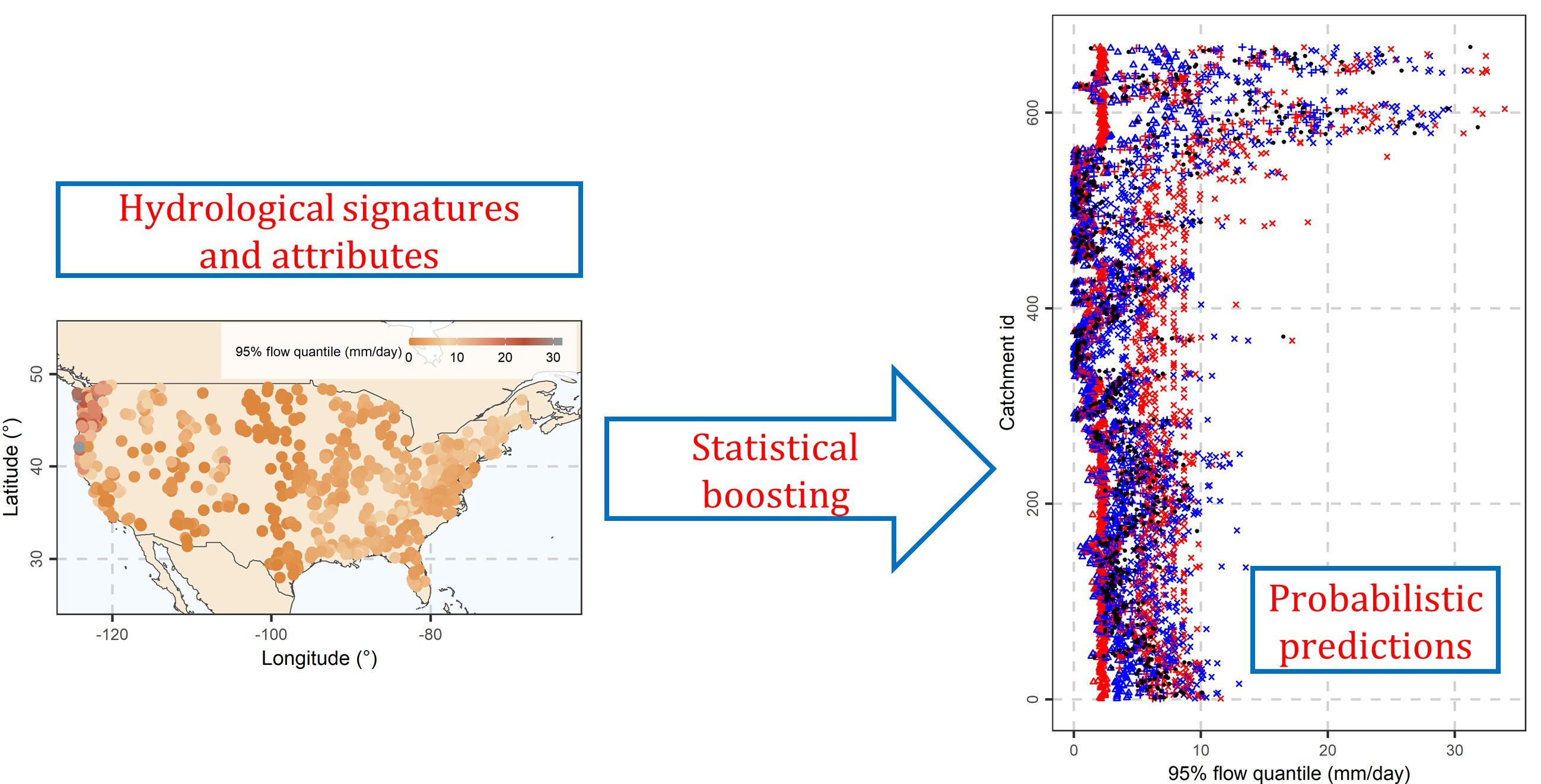
Explanation and Probabilistic Prediction of Hydrological Signatures with Statistical Boosting Algorithms

by
Hristos Tyralis
1,2,*,
Georgia Papacharalampous
3,4,
Andreas Langousis
3 and
Simon Michael Papalexiou
5,6,7
1
Hellenic Air Force General Staff, Hellenic Air Force, Mesogion Avenue 227-231, 155 61 Cholargos, Greece
2
Department of Water Resources and Environmental Engineering, School of Civil Engineering, National Technical University of Athens, Iroon Polytechniou 5, 157 80 Zografou, Greece
3
Department of Civil Engineering, School of Engineering, University of Patras, University Campus, Rio, 26 504 Patras, Greece
4
Department of Engineering, Roma Tre University, 00154 Rome, Italy
5
Department of Civil, Geological and Environmental Engineering, University of Saskatchewan, Saskatoon, SK S7N 5A2, Canada
6
Global Institute for Water Security, Saskatoon, SK S7N 3H5, Canada
7
Faculty of Environmental Sciences, Czech University of Life Sciences, 165 00 Prague, Czech Republic
*
Author to whom correspondence should be addressed.
Submission received: 13 December 2020 / Revised: 14 January 2021 / Accepted: 17 January 2021 / Published: 20 January 2021
(This article belongs to the Special Issue Remote Sensing of Geo-Hydrological Process in an Arid Region)

Abstract

:
Hydrological signatures, i.e., statistical features of streamflow time series, are used to characterize the hydrology of a region. A relevant problem is the prediction of hydrological signatures in ungauged regions using the attributes obtained from remote sensing measurements at ungauged and gauged regions together with estimated hydrological signatures from gauged regions. The relevant framework is formulated as a regression problem, where the attributes are the predictor variables and the hydrological signatures are the dependent variables. Here we aim to provide probabilistic predictions of hydrological signatures using statistical boosting in a regression setting. We predict 12 hydrological signatures using 28 attributes in 667 basins in the contiguous US. We provide formal assessment of probabilistic predictions using quantile scores. We also exploit the statistical boosting properties with respect to the interpretability of derived models. It is shown that probabilistic predictions at quantile levels 2.5% and 97.5% using linear models as base learners exhibit better performance compared to more flexible boosting models that use both linear models and stumps (i.e., one-level decision trees). On the contrary, boosting models that use both linear models and stumps perform better than boosting with linear models when used for point predictions. Moreover, it is shown that climatic indices and topographic characteristics are the most important attributes for predicting hydrological signatures.

Graphical Abstract

1. Introduction

Hydrological signatures are estimates of statistics that are used to characterize streamflow time series [1,2]. The concept of hydrological signatures was first introduced and explicitly described in [3]. Relevant signature-based characterizations may be related, for example, to the average or the extreme streamflow behavior, while some guidelines for selecting hydrological signatures can be found in [2]. Examples of hydrological signatures include the mean flow, the total runoff ratio, the baseflow index, the number of flow peaks over a threshold, the time lag between rainfall and flow series and more [1].
Hydrological signatures are useful in ecological and hydrological applications, for instance as proxies of hydrological processes [1] or in hydrological simulations [4]. In particular they are selected with the aim to exploit information about the hydrological behavior, e.g., “to identify dominant processes, and to determine the strength, speed and spatiotemporal variability of the rainfall-runoff response” [2]. Applications of hydrological signatures include understanding hydrological processes in a given catchment, comparing hydrological observations against model outputs, and estimating hydrological similarity across time or space [2]. Multiple signatures can be ranked according to their importance in characterizing the hydrology of a region, e.g., in clustering applications [5].
Streamflow data are unavailable for most catchments ([6], p. 2). In the case of ungauged catchments, streamflow signatures can be predicted using remote sensing data in combination with hydrological models or statistical and machine learning algorithms (e.g., [6,7,8,9]). Predicting the behavior of ungauged catchments, i.e., predicting their signatures is a relevant problem of interest. Such predictions should be probabilistic, so that one can understand their uncertainties (e.g., [10,11,12,13,14]). Furthermore, it is important to know the relationships between attributes of catchments and hydrological signatures [15]. Machine learning regression algorithms have been used to predict hydrological signatures [16,17,18]. Probabilistic predictions of hydrological signatures using regression algorithms can be found in [16], where some variant of quantile regression forests seems to have been used [19,20]. The procedure to predict hydrological signatures in ungauged basins using regression algorithms includes the establishment of a relationship between the attributes of the basin (predictor/independent variables) and the hydrological signature (dependent variable). A key point is that the predictor variables are widely available through remote sensing data, unlike the dependent variable.
Machine and statistical learning regression algorithms are great in establishing reliable relationships due to their flexibility [21,22,23] and they have been used extensively in hydrology [24,25,26,27,28]. A key issue in their use is that there is a trade-off between flexibility and interpretability ([23], p. 25). A second issue is that possible spatial dependencies cannot be modelled directly by frequently used machine learning algorithms, albeit there are some advancements towards this direction.
Here we aim to predict hydrological signatures (in particular mean daily discharge, 5% flow quantile, 95% flow quantile, baseflow index, average duration of high-flow events, frequency of high-flow days, average duration of low-flow events, frequency of low-flow days, runoff ratio, streamflow precipitation elasticity, slope of the flow duration curve and mean half-flow date) using statistical boosting algorithms [29] in a regression setting. Boosting is an ensemble learning algorithm that aims to improve the predictive performance of weak base learners based on an iterative fitting procedure. We apply the algorithms to a dataset consisting of 667 basins in the contiguous US (CONUS). This dataset comprises 28 attributes (predictor variables, such as topographic characteristics and climatic indices) and 12 hydrological signatures (such as low and high flow quantiles).
Compared to other machine learning models, boosting algorithms can be more interpretable, as additive base learners (base learners are combined to form an ensemble learning algorithm) can be used to model the effects of the predictor variables. Furthermore, a variable and model selection procedure is applied, which is particularly important in settings with a high number of predictor variables. In spite of their interpretability, boosting algorithms still remain flexible. Properties of boosting algorithms can be found in [30]. Probabilistic predictions are provided (we note that a single study exists that delivers probabilistic predictions in a regression setting, despite the large interest in quantifying predictive uncertainty [16]), while compared to previous studies, a formal assessment of the quality of probabilistic predictions is also presented.
The remainder of this paper is structured as follows. Section 2 presents the dataset and methods used in the manuscript. Results are presented in Section 3, followed by their discussion in Section 4. The paper closes with conclusions and recommendations for future works in Section 5.

2. Data and Methods

Here we present the dataset, the implemented boosting algorithms, the performance metrics and an overview of the methodology. We address the problem of constructing a model that will take basin attributes as inputs and provide probabilistic predictions of hydrological signatures. To this end, a boosting regression algorithm is fitted to available data of catchments located in CONUS, and the quantile loss function is minimized. Furthermore, the predictive performance of the algorithm is assessed in a 10-fold cross-validation.

2.1. Data

We used the Catchment Attributes and MEteorology for Large-sample Studies (CAMELS) dataset [31], which includes 671 basins. This dataset is open and appropriate for benchmarking and investigations in large-sample hydrology studies [32]. Furthermore, it is appropriate for studying catchments with diverse characteristics (e.g., climatic and geological) due to the extended spatial coverage of CONUS. The data can be found online in [33,34]. Documentation of the data is available in [31,35].
We selected 667 basins (the remaining ones had missing values) which cover the entire CONUS, as presented in Appendix B. The basins are characterized by minimal human influence; consequently, the use of regression algorithms is a reasonable option for the analysis. The spatial coverage is representative of the large range of hydroclimatic conditions met in CONUS. An overview of the catchment attributes can be found in Table A1 and their explanation can be found in Appendix A. The catchment attributes include hydrological signatures as described in Table A2 (attributes were computed using data collected by Newman et al. [35]), topographic characteristics as described in Table A3 (attributes were computed using data from Newman et al. [35]), climatic indices as described in Table A4 (attributes were computed using data by Thornton et al. [36]), land cover characteristics as described in Table A5 (attributes were computed using Moderate Resolution Imaging Spectroradiometer (MODIS) data), soil characteristics as described in Table A6 (attributes were computed using data by Miller and White [37] and Pelletier et al. [38]) and geological characteristics as described in Table A7 (attributes were computed using data by Gleeson et al. [39] and Hartmann and Moosdorf [40]) related to the basin of interest.

2.2. Boosting Algorithms

We are interested in boosting for statistical modelling [41] and, in particular, in some further developments related to the interpretability of the model. These developments are summarized in [29]. The overall approach is related to a general gradient descent “boosting” paradigm developed for additive expansions and any loss function [42] (see Algorithm 1 for this formulation).
Algorithm 1 Formulation of the gradient boosting algorithm, adapted from [29,30,42,43].
Step 1: Initialize f0 with a constant.
Step 2: For m = 1 to M:
a. Compute the negative gradient gm(xi) of the loss function L at fm–1(xi), i = 1, …, n.
b. Fit a new base learner function hm(x) to {(xi, gm(xi))}, i = 1, …, n.
c. Update the function estimate fm(x) ← fm–1(x) + ρ hm(x).
Step 3: Predict fM(x).
Here M is the number of iterations, hm(x) is the base learner fitted at each iteration and ρ is the step-length factor. Explanation of the role of parameters M and ρ can be found in the following.
An intuitive explanation of the concept of statistical boosting can be found in [44]. Statistical boosting can be seen as an algorithm to fit a regression model. Two properties of statistical boosting are typical. The first one, is that one can model the effect of each predictor variable (i.e., an element of the vector xi; see Algorithm 1) using simultaneously different base learners, e.g., linear models or decisions trees (commonly base learners are weak regression algorithms, i.e., they can predict slightly better than random guessing). The second one is that statistical boosting is in essence a function approximation procedure; therefore, diverse loss functions can be used to fit a model and assess the degree of approximation. Benefits related to the above two properties and the iterative fitting procedure of Algorithm 1 [44,45] are related to our problem.
Regarding the iterative procedure of statistical boosting, the final fitted model is additive with respect to the implemented base learners; therefore, it allows straightforward interpretation [46]. In addition, a base learner can be used multiple times, while a predictor variable can be modelled simultaneously by diverse base learners. The procedure of Algorithm 1 will decide how many times each predictor variable and each base learner will be included in the final additive model (we note that at step m, various base learners hm(x) can be applied, e.g., a linear model or a smooth function, however a single base learner will be selected, i.e., the one that minimizes the fitting error). Thus, statistical boosting performs simultaneously variable and model selection [47]. Variable selection is particularly important in the presence of multiple predictor variables (and more relevant in the context of high-dimensional problems [48,49,50]), while model selection is important when one does not know the type of appropriate model for the problem at hand.
Regarding the flexibility on the choice of loss functions, one may be interested in average properties of the dependent variable, in which case the L2 (squared error) loss function may be preferable amongst others [51]. In case one is interested in probabilistic predictions, the quantile loss function is appropriate (see Section 2.4).
Another important property of statistical boosting algorithms is that they are robust against multicollinearity issues due to regularizing the estimates of f using shrinkage techniques [44,52]. This property is important in the presence of a high number of predictor variables and in the context of high-dimensional problems.
The most important parameter to be estimated in statistical boosting is the number of boosting iterations M. A low number of iterations may result in underfitting, while a high number of iterations may result in overfitting. The optimal value of M can be estimated with k-fold cross validation in which the empirical risk, i.e., the loss function averaged over the observations, is minimized [52]. In particular, the early stopping optimizes predictive performance by regularizing the estimates of f using shrinkage techniques [52]. The value of ρ is of minor importance, while small values are preferable. Setting a small ρ, effect estimates increase “slowly” in the boosting procedure, and they stop increasing after the optimal stopping iteration. Here we set ρ = 1 [52].
Here, boosting algorithms were applied using the R programming implementations by [52,53]. The mboost R package implements model-based boosting methods, while its modular nature allows it to combine diverse base learners and loss-functions.

2.3. Base Learners

Boosting algorithms are designed to improve the predictive performance of weak base learners based on the iterative framework of Algorithm 1, in the sense that weak base learners are boosted to become strong ones [54]. Here we used linear models and stumps (i.e., one-level decision trees) to model basin attributes. Geographical coordinates were not explicitly modelled, because part of this information is included in other basin attributes. The idea of using simple models to model basin attributes is consistent with the basic concept of boosting algorithms.

2.4. Metrics

Our boosting algorithms were implemented by minimizing the quantile loss function proposed by [55]. At level a ∈ (0, 1), the quantile loss function imposes a penalty equal to L(r; x) to a prediction quantile r, when x materializes according to Equation (1):
L(r; x): = (rx) (𝟙(xr)−a),
where 𝟙(∙) denotes the indicator function.
The quantile loss function is a proper scoring rule [56] and is especially useful when one aims to predict conditional quantiles. It is related to linear-in-parameters quantile regression (i.e., linear regression with quantile loss) [57,58]. Interval scores [59,60] are special cases of quantile losses and are particularly useful when one provides prediction intervals, but here we aim to evaluate separately predictive quantiles. The value of quantile regressions in hydrology has been highlighted in [61].

2.5. Summary of Methods

Here we summarize the framework of our study. Firstly, selected attributes and signatures are transformed using the logarithm or the square root function before performing any computations. The selection of those attributes and signatures is based on some preliminary exploratory data analysis that seeks for possibly skewed data and aims to approximately normalize the data. The inverse transform is applied to all final predictions, and all results on predictive performance are reported with respect to back-transformed values. We note here that data preprocessing is a purely empirical procedure aiming to improve predictive ability of the algorithm. A summary of variables that are transformed can be found in Section 2.1.
The sample of 667 basins is divided randomly into 10 folds. Then the boosting algorithm is trained in nine folds and tested in the remaining fold. The procedure is repeated 10 times, so that all folds are included in the test set. All predictive performances are reported for the test set.
Now assume that one aims to predict a specific hydrological signature at all basins included in a single random fold. The boosting algorithm is trained in the remaining nine folds in a 10-fold cross-validation framework (this 10-fold cross-validation aims to estimate the optimal stopping parameter M and should not be confused with the 10-fold cross-validation mentioned in the previous paragraph). The procedure terminates in 2000 iterations. Predictions of negative sign are transformed to 0, for hydrological signatures that are known to be a priori positive (e.g., frequency of high-flow days).
Two cases are examined, i.e., boosting (a) using linear models to model each predictor variable and (b) using a linear model and a stump to model each predictor variable. The predictive performances of both boosting algorithms on the test set are reported for quantile levels equal to 2.5%, 50.0% and 97.5%. Furthermore, the procedure (b) (see paragraph above) is repeated by fitting the boosting algorithm in the full sample in a 10-fold cross-validation and the frequency of included predictor variables in the final model (i.e., the model obtained by implementing the optimal parameter M) is reported for providing an explanatory model.

3. Results

Here we present the results of the fitting problems. In particular, we provide some exploratory analysis in Section 3.1. Section 3.2, Section 3.3 and Section 3.4 present the probabilistic predictions for three categories of hydrological signatures, each one including four hydrological signatures from Table A1. An overall assessment of the implemented methods is presented in Section 3.5.

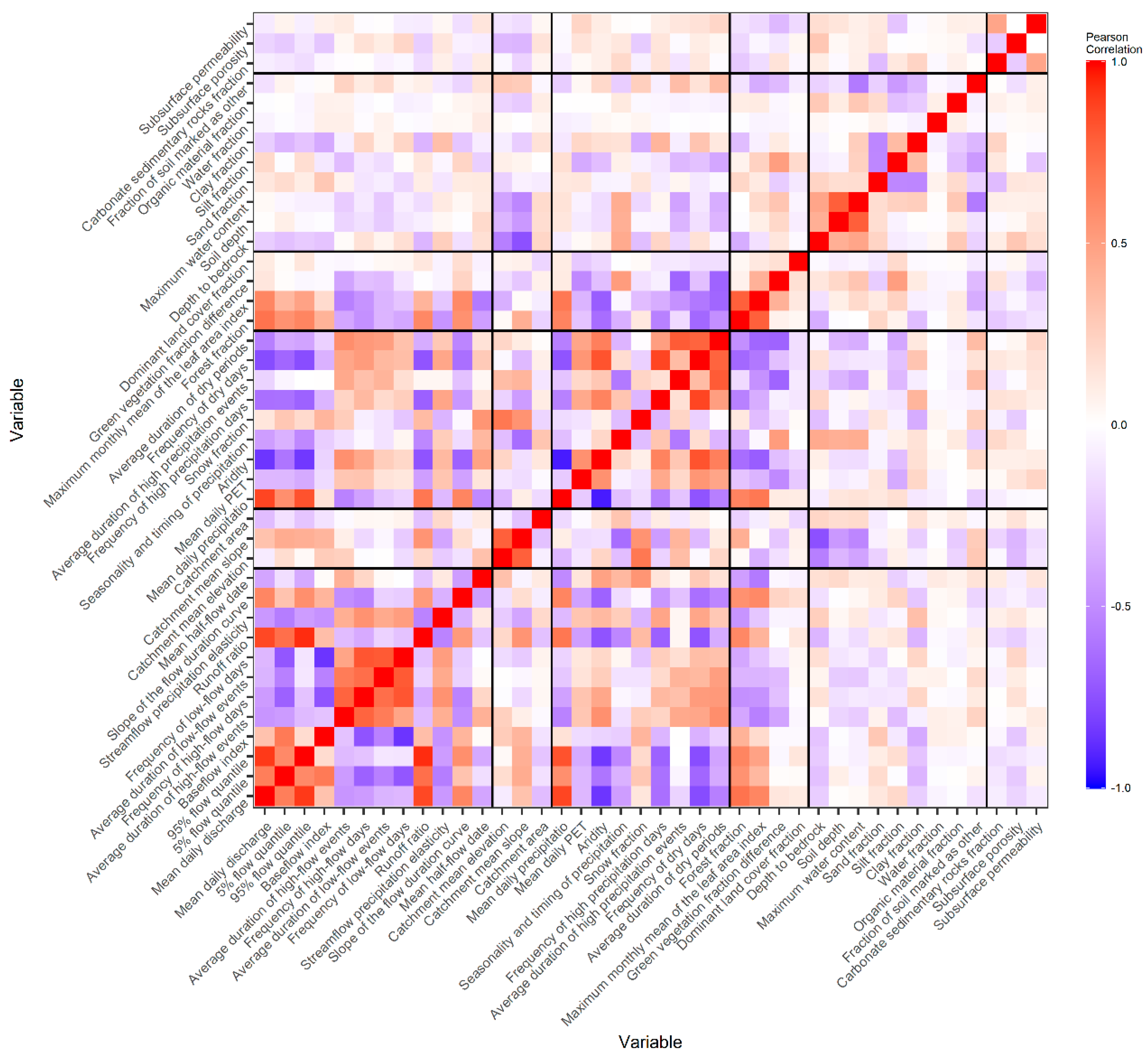
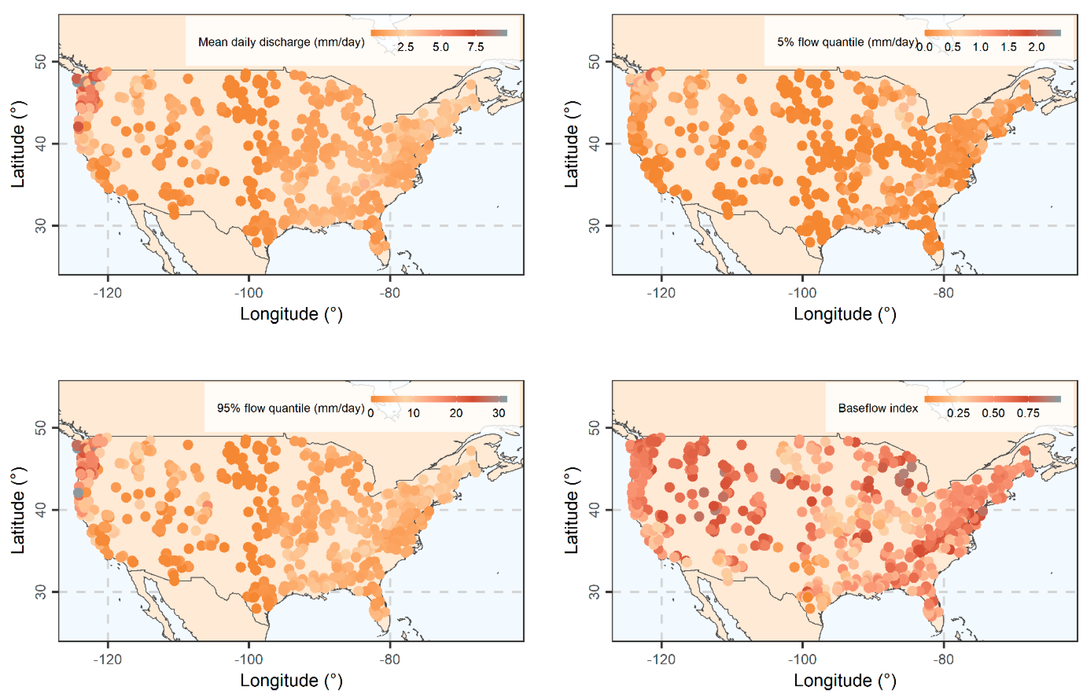
3.1. Exploratory Analysis

It is important to understand the relationships between hydrological signatures and basin attributes. To this end, a correlogram between all variables is presented in Figure 1. Most features are relatively uncorrelated. Regarding a few correlated variables, we note that statistical boosting can discriminate important variables with little consequence on predictive performance, due to its internal mechanism.
To better understand what Figure 1 depicts, we here note that variables were sorted according to their type (in both the horizontal and vertical directions); see Table A1. As regards the horizontal direction, hydrological signatures are placed in the bottom-left corner of Figure 1, being followed by climatic indices and the remaining types of variables (as we move from the left to the right). Some hydrological signatures are highly correlated (e.g., mean daily discharge, 5% flow quantile, 95% flow quantile and baseflow index). This does not pose problems for our approach, because hydrological signatures are modelled separately.
Another important note on Figure 1 is that possible low correlations between attributes and hydrological signatures may explain potential low predictability of the signatures. Consequently, estimating the uncertainty of the predictions is important. We also note that Pearson’s correlation is a linear metric; therefore, selection frequency of predictor variables given by boosting algorithms (see Section 3.5) may not be identical to a ranking of predictor variables according to the magnitude of Pearson’s correlation.

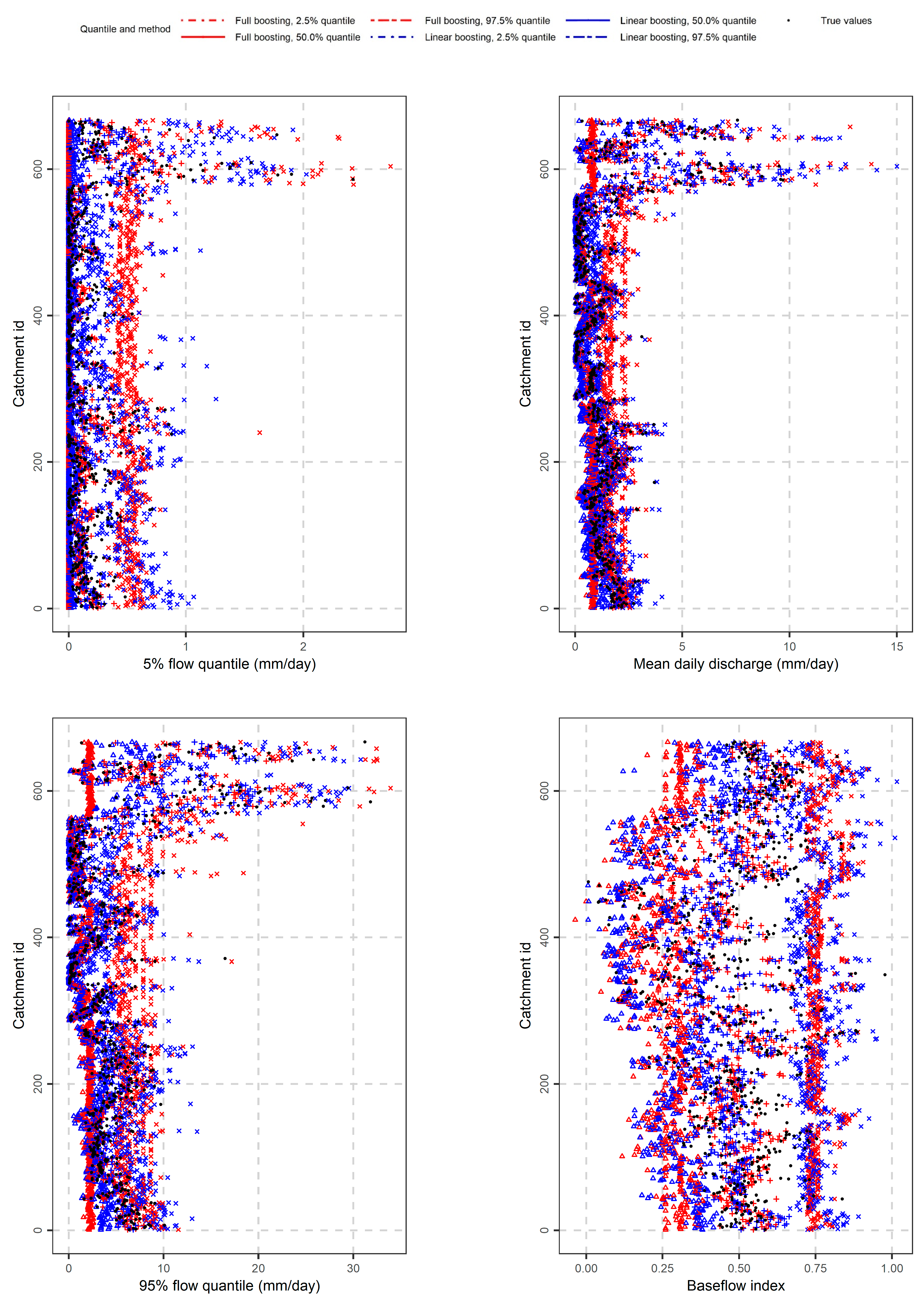
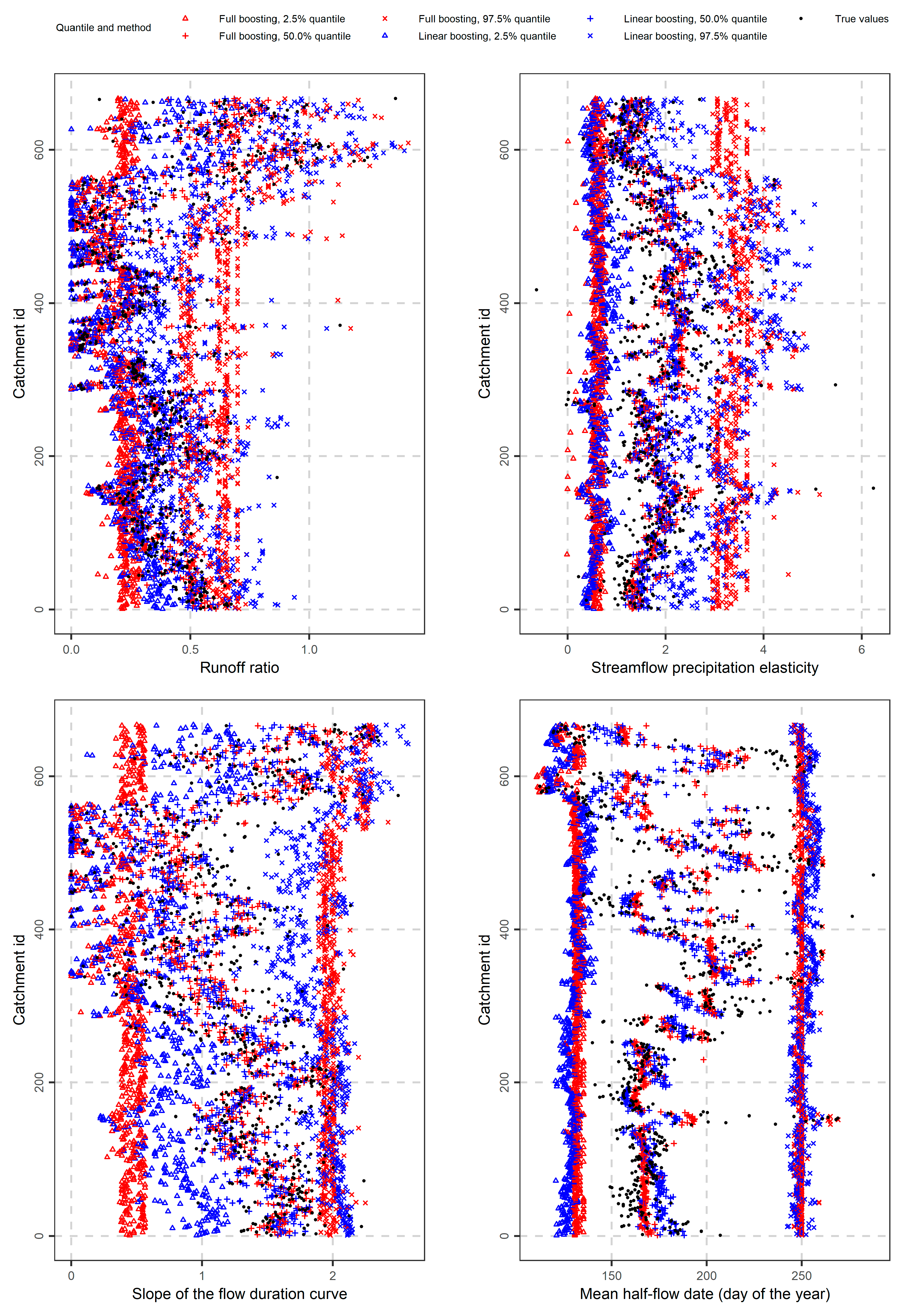
3.2. Streamflow Signatures

Here we present probabilistic predictions of signatures related to discharge volumes, i.e., mean daily discharge, 5% flow quantile, 95% flow quantile and baseflow index at quantile levels 2.5%, 50.0% and 95.0% in a 10-fold cross-validation procedure for the full sample of catchments. Similar analysis for the remaining signatures is presented in Section 3.3 and Section 3.4. Values of the variables are presented in Figure A1, while probabilistic predictions are presented in Figure 2. Two cases are examined, i.e., boosting with linear models as base learners and boosting with a combination of linear models and stumps as base learners. We note that 5% and 95% flow quantiles should not be confused with their 2.5%, 50.0% and 97.5% prediction quantiles. In particular, the problem is set so as to provide 2.5%, 50.0% and 97.5% prediction quantiles for 5% and 95% flow quantile hydrological signatures.
In general, we observe that predictions at quantile level 50% (i.e., predictions that aim to minimize the mean absolute error with respect to the observations) approximate well the observations. Moreover, prediction intervals seem to contain observed values for both implemented algorithms. It seems that both algorithms can provide probabilistic predictions that, in general, agree with the spatial heteroscedastic nature (i.e., the large and diverse variations) of the dependent variables. For instance, in catchments with high mean daily discharge the predictive quantiles at level 97.5% are also high. We note that predictive quantiles at level 2.5% seem not to follow the fluctuations of the observations. This is more evident in predictions of the 5% flow quantile and is due to the truncation at 0. Furthermore, boosting with linear models seems to be smoother with regards to model heterogeneity compared to boosting with linear models and stumps. For instance, when looking at the 97.5% predictive quantiles of the 5% flow quantile, boosting with linear models and stumps seems to provide less efficient variable predictions compared to boosting with linear models. A formal assessment of both algorithms using proper scoring rules will be presented in Section 3.5.

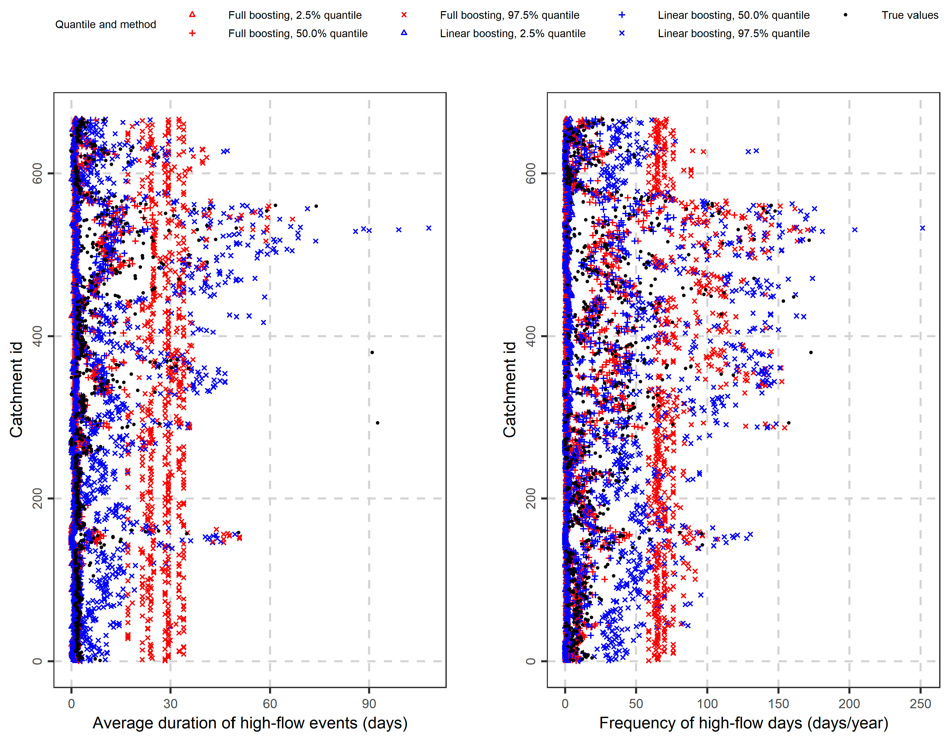
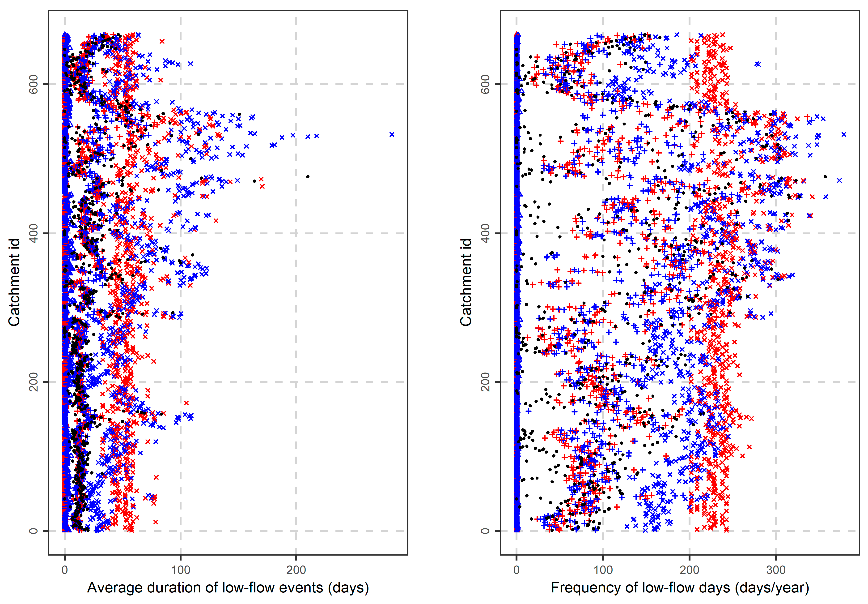
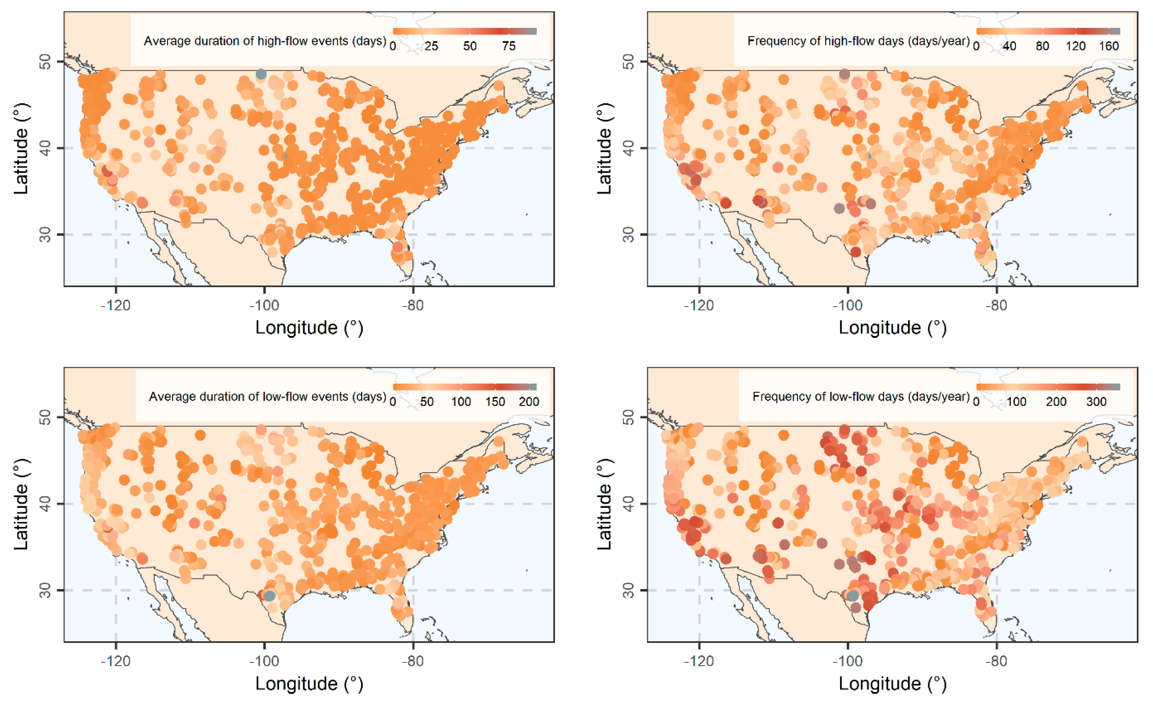
3.3. Signatures of Duration and Frequency of Extreme Events

Maps of values of high-flow events, frequency of high flow events, average duration of low-flow events and frequency of low-flow days are presented in Figure A2, while the respective probabilistic predictions are presented in Figure 3. Similar results as those reported in Section 3.2 regarding the comparison between the two implemented algorithms also hold here in the 10-fold cross-validation. In particular, signatures are well predicted by both algorithms, while prediction intervals contain the observed values. Boosting with linear models and stumps as base learners seems to be less variable at the 97.5% quantile level while the truncation effect at 0 is also evident.

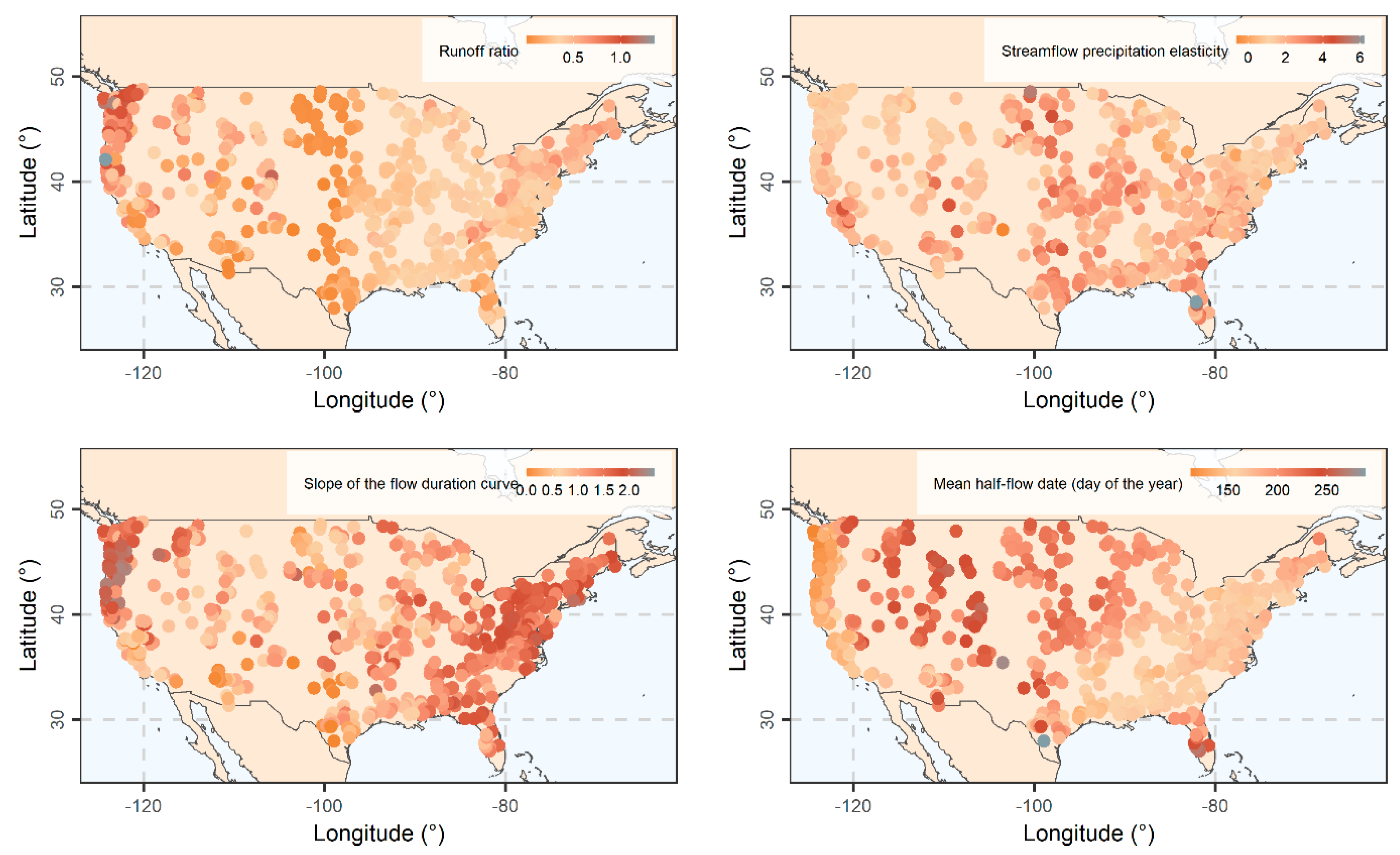
3.4. Remaining Signatures

Remaining signatures include runoff ratio, streamflow precipitation elasticity, slope of the flow duration curve and mean half-flow date as presented in Figure A3, while respective probabilistic predictions are presented in Figure 4. While similar results to Section 3.2 and Section 3.3 also hold here, we note that heteroscedasticity of mean half-flow date is not well predicted, since both algorithms seems to give predictions that are relatively constant at quantile levels 2.5% and 97.5%.

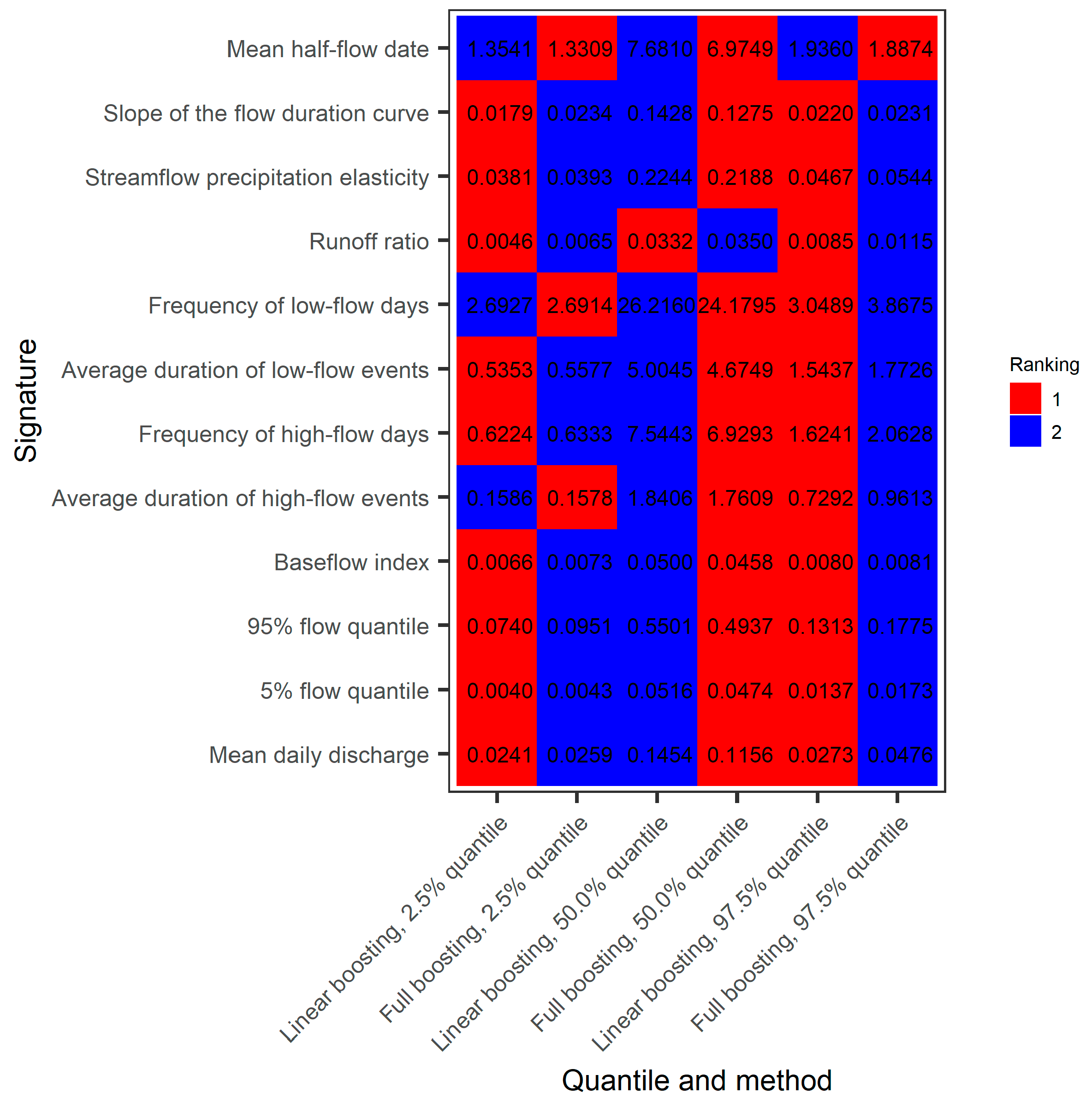
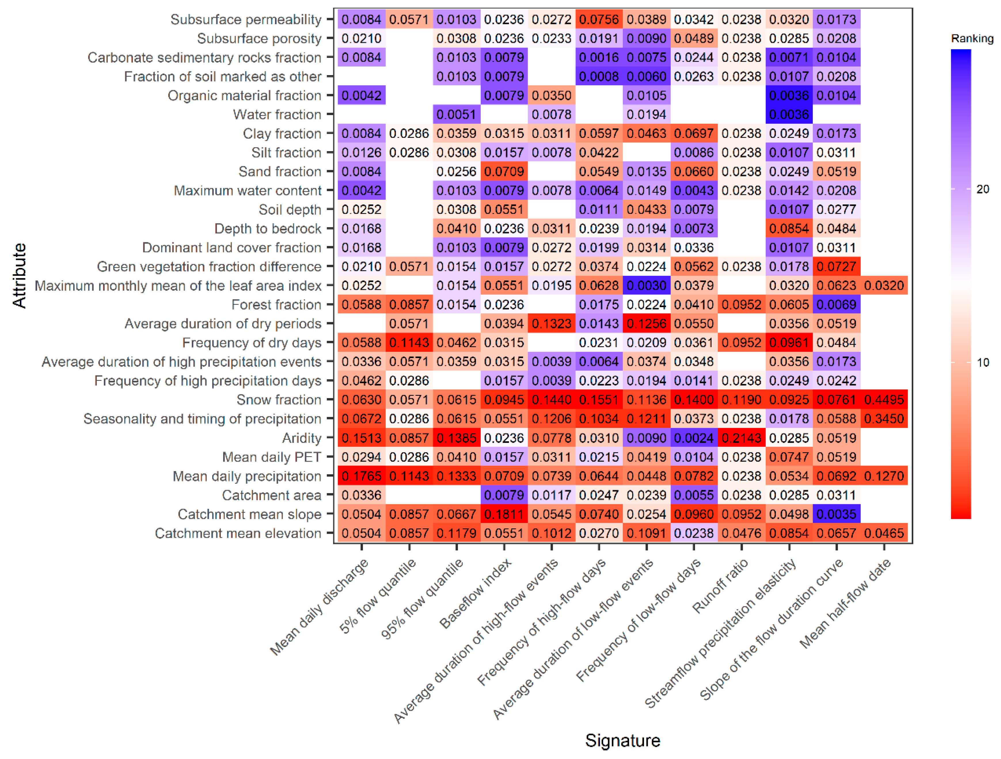
3.5. Assesment and Importance of Predictor Variables

Figure 5 presents an assessment of both algorithms in predicting hydrological signatures at 2.5%, 50.0% and 97.5% quantile levels in a 10-fold cross-validation framework. At quantile levels 2.5% and 97.5%, boosting with linear models as base learners seems to perform better than boosting with linear models and stumps as base learners. On the other hand, the combination of linear models and stumps as base learners seems to provide better results when the interest is in point predictions of hydrological signatures.
We are interested in obtaining some explainable models when predicting hydrological signatures. To this end, we fitted a statistical boosting model with linear models and stumps as base learners to predict a given hydrological signature at quantile level 50.0%. The final fitted model, i.e., the model with the optimal number of iterations (i.e., the model provided when trained in the full sample in a 10-fold cross-validation) includes predictor variables in frequencies reported in Figure 6. The procedure is repeated for every hydrological signature.
To understand Figure 6, we note that attributes in the vertical axis are reported with regards to their type, i.e., topographic characteristics, climatic indices, land cover characteristics, soil characteristics and geological characteristics (from lower to upper). In general, topographic characteristics and climatic indices seem to be most important when predicting hydrological signatures. Further discussion on the results of Figure 6 related to the selection frequency of the predictor variables can be found in Section 4.

4. Discussion

We note here that interpretation and accurate prediction in algorithmic modelling may be two conflicting objectives [62,63]. Therefore, some concessions should be accepted, since there is no free lunch in modelling [64], so that one obtains a model that provides acceptable predictions and is interpretable simultaneously. For instance, one could combine multiple models and obtain more accurate points [65,66] or probabilistic [67,68] predictions. However, in this case, interpretability would be lost for the sake of generalization. Furthermore, one could also use several models and compare them (see a discussion on the value of doing multiple comparisons using big datasets in general [69], and in hydrology in particular [70,71]). An example of comparison of multiple regression algorithms for providing point predictions of hydrological signatures can be found in [18]. Here we focus on exploiting the benefits of statistical boosting and we are less interested in comparing multiple algorithms.
With regards to studies providing probabilistic predictions of hydrological signatures, we note that [16] used some variant of quantile regression forests (which belong to the wider class of random forests algorithms). Compared to random forests, statistical boosting can be more interpretable. In particular, random forests use variable importance metrics to measure the relative importance of predictor variables in explaining the dependent variable [72]. On the other hand, statistical boosting is additive with respect to the predictor variables (which are modelled by linear regression algorithms), while their importance can be related to the frequency of the appearance of the predictor variables in the final model (see Figure 6). The finding that climatic indices are the most important variables for predicting hydrological signatures, is also confirmed by an earlier study [16]. We note that compared to [16], here a formal assessment of probabilistic predictions is provided based on quantile losses.
Uncertainties of hydrological signatures are provided by [13,14] using Monte Carlo sampling; however, the approach is not based on regression algorithms and the focus is to characterize distributional properties of hydrological signatures.
Moreover, regarding the properties of the implemented algorithm related to the problem at hand, we note that boosting performs model selection in the sense that the model is not known a priori and, therefore, several models are tried (e.g., linear models and stumps for each base learner) and boosting selects the most informative ones. This problem is especially relevant when many predictor variables exist. We also note that boosting with linear models is better than boosting with linear models and stumps for probabilistic predictions, perhaps due to the structure of stumps, which does not allow for optimal probabilistic modelling. On the other hand, most flexible models that include both linear models and stumps seem to perform better for point predictions, i.e., prediction at the 50.0% quantile level.
Regarding the importance of attributes for predicting hydrological signatures, snow fraction seems to be very important for predicting hydrological signatures, based on the number of red coloured tiles in Figure 6. The significance of snow fraction for the prediction of hydrological signatures has also been merely discussed by [16]. Catchment mean slope and catchment mean elevation (topographic characteristics) are also generally very important, based on the same criterion. Catchment mean slope and catchment mean elevation are highly correlated and, therefore, if one characteristic is omitted the other one may gain more importance. Mean daily precipitation (i.e., another climatic index) is also important.
Beyond topographic attributes and climatic indices, clay fraction (a soil characteristic), maximum monthly mean of the leaf area index (a land cover characteristic), forest fraction (another land cover characteristic) also seem to be important. Geological characteristics seem to not be particularly useful for predicting hydrological signatures. We note that these findings hold for the examined sample and, therefore, perhaps a different summarization of geological or other type of information may result in completely different conclusions. Among the examined hydrological signatures, the 5% flow quantile, runoff ratio, and the mean half-flow date seem to depend on fewer attributes (see Figure 6) compared to alternative hydrological signatures.

5. Conclusions

We provided probabilistic predictions at quantile levels 2.5%, 50.0% and 97.5% of 12 hydrological signatures, namely (1) mean daily discharge, (2) 5% flow quantile, (3) 95% flow quantile, (4) baseflow index, (5) average duration of high-flow events, (6) frequency of high-flow days, (7) average duration of low-flow events, (8) frequency of low-flow days, (9) runoff ratio, (10) streamflow precipitation elasticity, (11) slope of the flow duration curve and (12) mean half-flow date using statistical boosting in a regression setting. The sample includes 28 predictor variables, i.e., attributes of 667 basins in the contiguous US. Two boosting models were tested, i.e., (a) a model with linear models as base learners, and (b) a model with both linear models and stumps as base learners. Boosting modes were trained to minimize quantile loss at levels 2.5%, 50.0% and 97.5%.
Regarding prediction performances, model (a) provided better predictions at quantile levels 2.5% and 97.5%, while model (b) showed better performance in providing predictions at quantile level 50.0% (i.e., better point predictions). Boosting models can be more interpretable compared to other machine learning regression algorithms. By exploiting this latter property of theirs, we found that climatic indices and topographic characteristics are better predictors of hydrological signatures than characteristics of other types.
Uncertainty estimation of hydrological signatures is the focus of some published studies; however, a formal assessment of delivered results is missing. In particular, most studies use visual tools (e.g., q-q plots) or estimate reliability and coverages; however, a “proper scoring rule” (which may combine properties of reliability scores and coverages) can be more informative when the interest is in ranking probabilistic predictions. Machine learning algorithms can provide probabilistic predictions if designed to minimize some type of proper score (e.g., quantile scores and intervals scores), while delivered results can be more accurate compared to simple linear models, due to the flexibility of machine learning algorithms. Future work can include a comparison of more probabilistic regression models, as well as their combinations for providing more accurate predictions.

Author Contributions

Conceptualization, H.T. and G.P.; analysis, H.T.; visualizations, H.T. and G.P.; writing—original draft preparation, H.T.; writing—review, suggestions and enrichments, G.P., A.L. and S.M.P. All authors have read and agreed to the published version of the manuscript.

Funding

This research received no external funding.

Institutional Review Board Statement

Not applicable.

Informed Consent Statement

Not applicable.

Data Availability Statement

Raw data are publicly available; please see Section 2.1.

Acknowledgments

We thank the Editor for handling the review process and the reviewers whose comments helped us to improve the manuscript substantially.

Conflicts of Interest

We declare no conflict of interest.

Appendix A

Table A1 provides an overview of the selected basin features examined in the study.
Table A1. Predictor (topographic, climatic, land cover, soil and geology attributes) and dependent (hydrological) variables of the 667 basins obtained from [31], classified according to the transformation applied to them for being imported in the statistical boosting framework. A detailed description of the variables can be found in Table A2, Table A3, Table A4, Table A5, Table A6 and Table A7.
Type of VariablesValue as Is (Untransformed)Transformed Using LogTransformed Using Square Root
AttributeAttributeAttribute
SignatureBaseflow indexMean daily discharge5% flow quantile
Runoff ratio 95% flow quantile
Streamflow precipitation elasticity Average duration of high-flow events
Slope of the flow duration curve Frequency of high-flow days
Mean half-flow date Average duration of low-flow events
Frequency of low-flow days
Topographic Catchment mean elevation
Catchment mean slope
Catchment area
ClimaticSeasonality and timing of precipitationMean daily precipitation
Snow fractionMean daily PET
Frequency of high precipitation eventsAridity
Average duration of high precipitation eventsFrequency of dry days
Average duration of dry periods
Land coverForest fraction
Maximum monthly mean of the leaf area index
Green vegetation fraction difference
Dominant land cover fraction
SoilDepth to bedrock
Soil depth
Maximum water content
Sand fraction
Silt fraction
Clay fraction
Water fraction
Organic material fraction
Fraction of soil marked as other
GeologyCarbonate sedimentary rock fraction
Subsurface porosity
Subsurface permeability
In Table A2, Table A3, Table A4, Table A5, Table A6 and Table A7 we describe the signatures and attributes of the basins.
Table A2. Hydrological signatures computed over the period 1989/10/01 to 2009/09/30 (adapted from [31]).
AttributeDescription
Mean daily dischargeMean daily discharge (mm/day)
5% flow quantile5% flow quantile (low flow, mm/day)
95% flow quantile95% flow quantile (high flow, mm/day)
Baseflow indexRatio of mean daily baseflow to mean daily discharge, hydrograph separation using Landson et al. (2013) digital filter
Average duration of high-flow eventsNumber of consecutive days >9 times the median daily flow (days)
Frequency of high-flow daysFrequency of high-flow days (>9 times the median daily flow) (days/year)
Average duration of low-flow eventsNumber of consecutive days <0.2 times the mean daily flow (days)
Frequency of low-flow eventsFrequency of low-flow days (<0.2 times the mean daily flow (days/year)
Runoff ratioRatio of mean daily discharge to mean daily precipitation
Streamflow precipitation elasticityStreamflow precipitation elasticity (sensitivity of streamflow to changes in precipitation at the annual time scale)
Slope of the flow duration curveSlope of the flow duration curve (between the log-transformed 33rd and 66th streamflow percentiles)
Mean half-flow dateDate on which the cumulative discharge since October first reaches half of the annual discharge (day of year)
Table A3. Topographic characteristics (adapted from [31]).
AttributeDescription
Catchment mean elevationCatchment mean elevation (m)
Catchment mean slopeCatchment mean slope (m km–1)
Catchment areaCatchment area (GAGESII estimate) (km2)
Table A4. Climatic indices (adapted from [31]).
AttributeDescription
Mean daily precipitationMean daily precipitation (mm day–1)
Mean daily PETMean daily PET, estimated by N15 using Priestley–Taylor formulation calibrated for each catchment (mm day–1)
AridityAridity (PET/P, ratio of mean PET, estimated by N15 using Priestley–Taylor formulation calibrated for each catchment, to mean precipitation)
Seasonality and timing of precipitationSeasonality and timing of precipitation (estimated using sine curves to represent the annual temperature and precipitation cycles; positive (negative) values indicate that precipitation peaks in summer (winter); values close to 0 indicate uniform precipitation throughout the year)
Snow fractionFraction of precipitation falling as snow (i.e., on days colder than 0 °C)
Frequency of high precipitation eventsFrequency of high precipitation days (≥5 times mean daily precipitation) (days year–1)
Average duration of high precipitation eventsAverage duration of high precipitation events (number of consecutive days ≥5 times mean daily precipitation) (days)
Frequency of dry daysFrequency of dry days (<1 mm day–1) (days year–1)
Average duration of dry eventsAverage duration of dry periods (number of consecutive days < 1 mm day–1) (days)
Table A5. Land cover characteristics (adapted from [31]).
AttributeDescription
Forest fractionForest fraction
Maximum monthly mean of the leaf area indexMaximum monthly mean of the leaf area index (based on 12 monthly means)
Green vegetation fraction differenceDifference between the maximum and minimum monthly mean of the green vegetation fraction (based on 12 monthly means)
Dominant land cover fractionFraction of the catchment area associated with the dominant land cover
Table A6. Soil characteristics (adapted from [31]).
AttributeDescription
Depth to bedrockDepth to bedrock (maximum 50 m) (m)
Soil depthSoil depth (maximum 1.5 m; layers marked as water and bedrock were excluded) (m)
Maximum water contentMaximum water content (combination of porosity and soil_depth_statsgo; layers marked as water, bedrock, and “other” were excluded) (m)
Sand fractionSand fraction (of the soil material smaller than 2 mm; layers marked as organic material, water, bedrock, and “other” were excluded) (%)
Silt fractionSilt fraction (of the soil material smaller than 2 mm; layers marked as organic material, water, bedrock, and “other” were excluded) (%)
Clay fractionClay fraction (of the soil material smaller than 2 mm; layers marked as organic material, water, bedrock, and “other” were excluded) (%)
Water fractionFraction of the top 1.5 m marked as water (class 14) (%)
Organic material fractionFraction of soil_depth_statsgo marked as organic material (class 13) (%)
Fraction of soil marked as otherFraction of soil_depth_statsgo marked as “other” (class 16) (%)
Table A7. Geological characteristics (adapted from [31]).
AttributeDescription
Carbonate sedimentary rocks fractionFraction of the catchment area characterized as “carbonate sedimentary rocks”
Subsurface porositySubsurface porosity
Subsurface permeabilitySubsurface permeability (log10) (m2)

Appendix B

Figure A1, Figure A2 and Figure A3 present the geographic location of the basins included in the dataset and values of their respective hydrological signatures.
Figure A1. Maps of values of mean daily discharge, 5% flow quantile, 95% flow quantile and baseflow index; see also the analysis in Section 3.2.
Remotesensing 13 00333 g0a1
Figure A2. Maps of values of high-flow events, frequency of high flow events, average duration of low-flow events and frequency of low-flow days; see also the analysis in Section 3.3.
Remotesensing 13 00333 g0a2
Figure A3. Maps of values of runoff ratio, streamflow precipitation elasticity, slope of the flow duration curve and mean half-flow date; see also the analysis in Section 3.4.
Remotesensing 13 00333 g0a3

Appendix C

We used the R programming language [73] to implement the algorithms of the study, and to report and visualize the results.
For data processing, we used the contributed R packages data.table [74], gdata [75], reshape2 [76,77], stringr [78].
The algorithms were implemented by using the contributed R packages caret [79], mboost [80].
Visualizations were made by using the contributed R package ggplot2 [81,82], wesanderson [83].
Reports were produced by using the contributed R packages devtools [84], knitr [85,86,87], rmarkdown [88,89].

References

  1. McMillan, H. Linking hydrologic signatures to hydrologic processes: A review. Hydrol. Process. 2020, 34, 1393–1409. [Google Scholar] [CrossRef]
  2. McMillan, H.; Westerberg, I.; Branger, F. Five guidelines for selecting hydrological signatures. Hydrol. Process. 2017, 31, 4757–4761. [Google Scholar] [CrossRef] [Green Version]
  3. Gupta, H.V.; Wagener, T.; Liu, Y. Reconciling theory with observations: Elements of a diagnostic approach to model evaluation. Hydrol. Process. 2008, 22, 3802–3813. [Google Scholar] [CrossRef]
  4. Shafii, M.; Tolson, B.A. Optimizing hydrological consistency by incorporating hydrological signatures into model calibration objectives. Water Resour. Res. 2015, 51, 3796–3814. [Google Scholar] [CrossRef] [Green Version]
  5. Papacharalampous, G.; Tyralis, H.; Papalexiou, S.M.; Langousis, A.; Khatami, S.; Volpi, E.; Grimaldi, S. Global-scale massive feature extraction from monthly hydroclimatic time series: Statistical characterizations, spatial patterns and hydrological similarity. Sci. Total Environ. 2021, 767, 144612. [Google Scholar] [CrossRef]
  6. Blöschl, G.; Sivapalan, M.; Wagener, T.; Viglione, A.; Savenije, H. Runoff Prediction in Ungauged Basins; Cambridge University Press: New York, NY, USA, 2013; ISBN 978-1-107-02818-0. [Google Scholar]
  7. Hrachowitz, M.; Savenije, H.H.G.; Blöschl, G.; McDonnell, J.J.; Sivapalan, M.; Pomeroy, J.W.; Arheimer, B.; Blume, T.; Clark, M.P.; Ehret, U.; et al. A decade of Predictions in Ungauged Basins (PUB)—A review. Hydrol. Sci. J. 2013, 58, 1198–1255. [Google Scholar] [CrossRef]
  8. Singh, R.; Archfield, S.A.; Wagener, T. Identifying dominant controls on hydrologic parameter transfer from gauged to ungauged catchments—A comparative hydrology approach. J. Hydrol. 2014, 517, 985–996. [Google Scholar] [CrossRef]
  9. Viglione, A.; Parajka, J.; Rogger, M.; Salinas, J.L.; Laaha, G.; Sivapalan, M.; Blöschl, G. Comparative assessment of predictions in ungauged basins—Part 3: Runoff signatures in Austria. Hydrol. Earth Syst. Sci. 2013, 17, 2263–2279. [Google Scholar] [CrossRef] [Green Version]
  10. Blöschl, G.; Bierkens, M.F.P.; Chambel, A.; Cudennec, C.; Destouni, G.; Fiori, A.; Kirchner, J.W.; McDonnell, J.J.; Savenije, H.H.G.; Sivapalan, M.; et al. Twenty-three Unsolved Problems in Hydrology (UPH)—A community perspective. Hydrol. Sci. J. 2019, 64, 1141–1158. [Google Scholar] [CrossRef] [Green Version]
  11. Bourgin, F.; Andréassian, V.; Perrin, C.; Oudin, L. Transferring global uncertainty estimates from gauged to ungauged catchments. Hydrol. Earth Syst. Sci. 2015, 19, 2535–2546. [Google Scholar] [CrossRef]
  12. Wagener, T.; Montanari, A. Convergence of approaches toward reducing uncertainty in predictions in ungauged basins. Water Resour. Res. 2011, 47, W06301. [Google Scholar] [CrossRef] [Green Version]
  13. Westerberg, I.K.; McMillan, H.K. Uncertainty in hydrological signatures. Hydrol. Earth Syst. Sci. 2015, 19, 3951–3968. [Google Scholar] [CrossRef] [Green Version]
  14. Westerberg, I.K.; Wagener, T.; Coxon, G.; McMillan, H.K.; Castellarin, A.; Montanari, A.; Freer, J. Uncertainty in hydrological signatures for gauged and ungauged catchments. Water Resour. Res. 2016, 52, 1847–1865. [Google Scholar] [CrossRef] [Green Version]
  15. Beck, H.E.; de Roo, A.; van Dijk, A.I.J.M. Global maps of streamflow characteristics based on observations from several thousand catchments. J. Hydrometeorol. 2015, 16, 1478–1501. [Google Scholar] [CrossRef]
  16. Addor, N.; Nearing, G.; Prieto, C.; Newman, A.J.; Le Vine, N.; Clark, M.P. A ranking of hydrological signatures based on their predictability in space. Water Resour. Res. 2018, 54, 8792–8812. [Google Scholar] [CrossRef]
  17. Tyralis, H.; Papacharalampous, G.; Tantanee, S. How to explain and predict the shape parameter of the generalized extreme value distribution of streamflow extremes using a big dataset. J. Hydrol. 2019, 574, 628–645. [Google Scholar] [CrossRef]
  18. Zhang, Y.; Chiew, F.H.S.; Li, M.; Post, D. Predicting runoff signatures using regression and hydrological modeling approaches. Water Resour. Res. 2018, 54, 7859–7878. [Google Scholar] [CrossRef]
  19. Breiman, L. Random forests. Mach. Learn. 2001, 45, 5–32. [Google Scholar] [CrossRef] [Green Version]
  20. Meinshausen, N. Quantile regression forests. J. Mach. Learn. Res. 2006, 7, 983–999. [Google Scholar]
  21. Efron, B.; Hastie, T. Computer Age Statistical Inference; Cambridge University Press: New York, NY, USA, 2016; ISBN 9781107149892. [Google Scholar]
  22. Hastie, T.; Tibshirani, R.; Friedman, J. The Elements of Statistical Learning; Springer: New York, NY, USA, 2009. [Google Scholar] [CrossRef]
  23. James, G.; Witten, D.; Hastie, T.; Tibshirani, R. An Introduction to Statistical Learning; Springer: New York, NY, USA, 2013. [Google Scholar] [CrossRef]
  24. Abrahart, R.J.; Anctil, F.; Coulibaly, P.; Dawson, C.W.; Mount, N.J.; See, L.M.; Shamseldin, A.Y.; Solomatine, D.P.; Toth, E.; Wilby, R.L. Two decades of anarchy? Emerging themes and outstanding challenges for neural network river forecasting. Prog. Phys. Geogr. Earth Environ. 2012, 36, 480–513. [Google Scholar] [CrossRef]
  25. Dawson, C.W.; Wilby, R.L. Hydrological modelling using artificial neural networks. Prog. Phys. Geogr. Earth Environ. 2001, 25, 80–108. [Google Scholar] [CrossRef]
  26. Solomatine, D.P.; Ostfeld, A. Data-driven modelling: Some past experiences and new approaches. J. Hydroinform. 2008, 10, 3–22. [Google Scholar] [CrossRef] [Green Version]
  27. Maier, H.R.; Jain, A.; Dandy, G.C.; Sudheer, K.P. Methods used for the development of neural networks for the prediction of water resource variables in river systems: Current status and future directions. Environ. Model. Softw. 2010, 25, 891–909. [Google Scholar] [CrossRef]
  28. Tyralis, H.; Papacharalampous, G.; Langousis, A. A brief review of random forests for water scientists and practitioners and their recent history in water resources. Water 2019, 11, 910. [Google Scholar] [CrossRef] [Green Version]
  29. Bühlmann, P.; Hothorn, T. Boosting algorithms: Regularization, prediction and model fitting. Stat. Sci. 2007, 22, 477–505. [Google Scholar] [CrossRef]
  30. Tyralis, H.; Papacharalampous, G. Boosting algorithms in energy research: A systematic review. arXiv 2020, arXiv:2004.07049v1. [Google Scholar]
  31. Addor, N.; Newman, A.J.; Mizukami, N.; Clark, M.P. The CAMELS data set: Catchment attributes and meteorology for large-sample studies. Hydrol. Earth Syst. Sci. 2017, 21, 5293–5313. [Google Scholar] [CrossRef] [Green Version]
  32. Newman, A.J.; Mizukami, N.; Clark, M.P.; Wood, A.W.; Nijssen, B.; Nearing, G. Benchmarking of a physically based hydrologic model. J. Hydrometeorol. 2017, 18, 2215–2225. [Google Scholar] [CrossRef]
  33. Addor, N.; Newman, A.J.; Mizukami, N.; Clark, M.P. Catchment Attributes for Large-Sample Studies; UCAR/NCAR: Boulder, CO, USA, 2017. [Google Scholar] [CrossRef]
  34. Newman, A.J.; Sampson, K.; Clark, M.P.; Bock, A.; Viger, R.J.; Blodgett, D. A Large-Sample Watershed-Scale Hydrometeorological Dataset for the Contiguous USA; UCAR/NCAR: Boulder, CO, USA, 2014. [Google Scholar] [CrossRef]
  35. Newman, A.J.; Clark, M.P.; Sampson, K.; Wood, A.; Hay, L.E.; Bock, A.; Viger, R.J.; Blodgett, D.; Brekke, L.; Arnold, J.R.; et al. Development of a large-sample watershed-scale hydrometeorological data set for the contiguous USA: Data set characteristics and assessment of regional variability in hydrologic model performance. Hydrol. Earth Syst. Sci. 2015, 19, 209–223. [Google Scholar] [CrossRef] [Green Version]
  36. Thornton, P.E.; Thornton, M.M.; Mayer, B.W.; Wilhelmi, N.; Wei, Y.; Devarakonda, R.; Cook, R.B. Daymet: Daily Surface Weather Data on a 1-km Grid for North America, Version 2; ORNL DAAC: Oak Ridge, TN, USA, 2014. [Google Scholar] [CrossRef]
  37. Miller, D.A.; White, R.A. A conterminous United States multilayer soil characteristics dataset for regional climate and hydrology modeling. Earth Interact. 1998, 2, 1–26. [Google Scholar] [CrossRef]
  38. Pelletier, J.D.; Broxton, P.D.; Hazenberg, P.; Zeng, X.; Troch, P.A.; Niu, G.-Y.; Williams, Z.; Brunke, M.A.; Gochis, D. A gridded global data set of soil, intact regolith, and sedimentary deposit thicknesses for regional and global land surface modeling. J. Adv. Modeling Earth Syst. 2016, 8, 41–65. [Google Scholar] [CrossRef]
  39. Gleeson, T.; Moosdorf, N.; Hartmann, J.; Beek, L.P.H. A glimpse beneath earth’s surface: GLobal HYdrogeology MaPS (GLHYMPS) of permeability and porosity. Geophys. Res. Lett. 2014, 41, 3891–3898. [Google Scholar] [CrossRef] [Green Version]
  40. Hartmann, J.; Moosdorf, N. The new global lithological map database GLiM: A representation of rock properties at the Earth surface. Geochem. Geophys. Geosyst. 2012, 13, Q12004. [Google Scholar] [CrossRef]
  41. Friedman, J.H.; Hastie, T.; Tibshirani, R. Additive logistic regression: A statistical view of boosting. Ann. Stat. 2000, 28, 337–407. [Google Scholar] [CrossRef]
  42. Friedman, J.H. Greedy function approximation: A gradient boosting machine. Ann. Stat. 2001, 29, 1189–1232. [Google Scholar] [CrossRef]
  43. Natekin, A.; Knoll, A. Gradient boosting machines, a tutorial. Front. Neurorobot. 2013, 7, 21. [Google Scholar] [CrossRef] [PubMed] [Green Version]
  44. Mayr, A.; Hofner, B. Boosting for statistical modelling: A non-technical introduction. Stat. Model. 2018, 18, 365–384. [Google Scholar] [CrossRef]
  45. Bühlmann, P.; Yu, B. Boosting. Wiley Interdiscip. Rev. Comput. Stat. 2010, 2, 69–74. [Google Scholar] [CrossRef]
  46. Mayr, A.; Binder, H.; Gefeller, O.; Schmid, M. The evolution of boosting algorithms. Methods Inf. Med. 2014, 53, 419–427. [Google Scholar] [CrossRef] [Green Version]
  47. Mayr, A.; Binder, H.; Gefeller, O.; Schmid, M. Extending statistical boosting. Methods Inf. Med. 2014, 53, 428–435. [Google Scholar] [CrossRef] [Green Version]
  48. Bühlmann, P. Boosting methods: Why they can be useful for high-dimensional data. In Proceedings of the 3rd International Workshop on Distributed Statistical Computing (DSC 2003), Vienna, Austria, 20–22 March 2003. [Google Scholar]
  49. Bühlmann, P. Boosting for high-dimensional linear models. Ann. Stat. 2006, 34, 559–583. [Google Scholar] [CrossRef] [Green Version]
  50. Hothorn, T.; Bühlmann, P. Model-based boosting in high dimensions. Bioinformatics 2006, 22, 2828–2829. [Google Scholar] [CrossRef] [PubMed] [Green Version]
  51. Bühlmann, P.; Yu, B. Boosting with the L2 loss. J. Am. Stat. Assoc. 2003, 98, 324–339. [Google Scholar] [CrossRef]
  52. Hofner, B.; Mayr, A.; Robinzonov, N.; Schmid, M. Model-based boosting in R: A hands-on tutorial using the R package mboost. Comput. Stat. 2014, 29, 1–35. [Google Scholar] [CrossRef] [Green Version]
  53. Hothorn, T.; Bühlmann, P.; Kneib, T.; Schmid, M.; Hofner, B. Model-based boosting 2.0. J. Mach. Learn. Res. 2010, 11, 2109–2113. [Google Scholar]
  54. Schapire, R.E. The strength of weak learnability. Mach. Learn. 1990, 5, 197–227. [Google Scholar] [CrossRef] [Green Version]
  55. Koenker, R.W.; Machado, J.A.F. Goodness of fit and related inference processes for quantile regression. J. Am. Stat. Assoc. 1999, 94, 1296–1310. [Google Scholar] [CrossRef]
  56. Gneiting, T.; Raftery, A.E. Strictly proper scoring rules, prediction, and estimation. J. Am. Stat. Assoc. 2007, 102, 359–378. [Google Scholar] [CrossRef]
  57. Koenker, R.W.; Bassett, G., Jr. Regression quantiles. Econometrica 1978, 46, 33–50. [Google Scholar] [CrossRef]
  58. Koenker, R.W. Quantile regression: 40 years on. Annu. Rev. Econ. 2017, 9, 155–176. [Google Scholar] [CrossRef] [Green Version]
  59. Dunsmore, I.R. A Bayesian approach to calibration. J. R. Stat. Society. Ser. B (Methodol.) 1968, 30, 396–405. [Google Scholar] [CrossRef]
  60. Winkler, R.L. A decision-theoretic approach to interval estimation. J. Am. Stat. Assoc. 1972, 67, 187–191. [Google Scholar] [CrossRef]
  61. Papacharalampous, G.; Tyralis, H.; Langousis, A.; Jayawardena, A.W.; Sivakumar, B.; Mamassis, N.; Montanari, A.; Koutsoyiannis, D. Probabilistic hydrological post-processing at scale: Why and how to apply machine-learning quantile regression algorithms. Water 2019, 11, 2126. [Google Scholar] [CrossRef] [Green Version]
  62. Breiman, L. Statistical modeling: The two cultures. Stat. Sci. 2001, 16, 199–231. [Google Scholar] [CrossRef]
  63. Shmueli, G. To explain or to predict? Stat. Sci. 2010, 25, 289–310. [Google Scholar] [CrossRef]
  64. Wolpert, D.H. The lack of a priori distinctions between learning algorithms. Neural Comput. 1996, 8, 1341–1390. [Google Scholar] [CrossRef]
  65. Papacharalampous, G.; Tyralis, H. Hydrological time series forecasting using simple combinations: Big data testing and investigations on one-year ahead river flow predictability. J. Hydrol. 2020, 590, 125205. [Google Scholar] [CrossRef]
  66. Tyralis, H.; Papacharalampous, G.; Langousis, A. Super ensemble learning for daily streamflow forecasting: Large-scale demonstration and comparison with multiple machine learning algorithms. Neural Comput. Appl. 2020. [Google Scholar] [CrossRef]
  67. Tyralis, H.; Papacharalampous, G.; Burnetas, A.; Langousis, A. Hydrological post-processing using stacked generalization of quantile regression algorithms: Large-scale application over CONUS. J. Hydrol. 2019, 577, 123957. [Google Scholar] [CrossRef]
  68. Papacharalampous, G.; Tyralis, H.; Koutsoyiannis, D.; Montanari, A. Quantification of predictive uncertainty in hydrological modelling by harnessing the wisdom of the crowd: A large-sample experiment at monthly timescale. Adv. Water Resour. 2020, 136, 103470. [Google Scholar] [CrossRef] [Green Version]
  69. Boulesteix, A.L.; Binder, H.; Abrahamowicz, M.; Sauerbrei, W. For the Simulation Panel of the STRATOS Initiative. On the necessity and design of studies comparing statistical methods. Biom. J. 2018, 60, 216–218. [Google Scholar] [CrossRef] [PubMed]
  70. Papacharalampous, G.; Tyralis, H.; Koutsoyiannis, D. Univariate time series forecasting of temperature and precipitation with a focus on machine learning algorithms: A multiple-case study from Greece. Water Resour. Manag. 2018, 32, 5207–5239. [Google Scholar] [CrossRef]
  71. Papacharalampous, G.; Tyralis, H.; Koutsoyiannis, D. Comparison of stochastic and machine learning methods for multi-step ahead forecasting of hydrological processes. Stoch. Environ. Res. Risk Assess. 2019, 33, 481–514. [Google Scholar] [CrossRef]
  72. Biau, G.; Scornet, E. A random forest guided tour. Test 2016, 25, 197–227. [Google Scholar] [CrossRef] [Green Version]
  73. R Core Team. R: A Language and Environment for Statistical Computing; R Foundation for Statistical Computing: Vienna, Austria, 2020; Available online: https://www.R-project.org/ (accessed on 13 December 2020).
  74. Dowle, M.; Srinivasan, A. Data.Table: Extension of ‘Data.Frame’. R Package Version 1.13. 2020. Available online: https://CRAN.R-project.org/package=data.table (accessed on 13 December 2020).
  75. Warnes, G.R.; Bolker, B.; Gorjanc, G.; Grothendieck, G.; Korosec, A.; Lumley, T.; MacQueen, D.; Magnusson, A.; Rogers, J. Gdata: Various R Programming Tools for Data Manipulation. R Package Version 2.18.0. 2017. Available online: https://CRAN.R-project.org/package=gdata (accessed on 13 December 2020).
  76. Wickham, H. reshape2: Flexibly Reshape Data: A Reboot of the Reshape Package. R Package Version 1.4.4. 2020. Available online: https://CRAN.R-project.org/package=reshape2 (accessed on 13 December 2020).
  77. Wickham, H. Reshaping data with the reshape package. J. Stat. Softw. 2007, 21, 1–20. [Google Scholar] [CrossRef]
  78. Wickham, H. stringr: Simple, Consistent Wrappers for Common String Operations. R Package Version 1.4.0. 2019. Available online: https://CRAN.R-project.org/package=stringr (accessed on 13 December 2020).
  79. Kuhn, M. caret: Classification and Regression Training. R Package Version 6.0-86. 2020. Available online: https://CRAN.R-project.org/package=caret (accessed on 13 December 2020).
  80. Hothorn, T.; Bühlmann, P.; Kneib, T.; Schmid, M.; Hofner, B. mboost: Model-Based Boosting. R Package Version 2.9-3. 2020. Available online: https://CRAN.R-project.org/package=mboost (accessed on 13 December 2020).
  81. Wickham, H. ggplot2; Springer: New York, NY, USA, 2016. [Google Scholar] [CrossRef]
  82. Wickham, H.; Chang, W.; Henry, L.; Pedersen, T.L.; Takahashi, K.; Wilke, C.; Woo, K.; Yutani, H.; Dunnington, D. ggplot2: Create Elegant Data Visualisations Using the Grammar of Graphics. R package Version 3.3.2. 2020. Available online: https://CRAN.R-project.org/package=ggplot2 (accessed on 13 December 2020).
  83. Ram, K.; Wickham, H. wesanderson: A Wes Anderson Palette Generator. R Package Version 0.3.6. 2018. Available online: https://CRAN.R-project.org/package=wesanderson (accessed on 13 December 2020).
  84. Wickham, H.; Hester, J.; Chang, W. devtools: Tools to Make Developing R Packages Easier. R Package Version 2.3.1. 2020. Available online: https://CRAN.R-project.org/package=devtools (accessed on 13 December 2020).
  85. Xie, Y. knitr: A comprehensive tool for reproducible research in R. In Implementing Reproducible Computational Research; Stodden, V., Leisch, F., Peng, R.D., Eds.; Chapman and Hall/CRC: Boca Raton, FL, USA, 2014. [Google Scholar]
  86. Xie, Y. Dynamic Documents with R and Knitr, 2nd ed.; Chapman and Hall/CRC: Boca Raton, FL, USA, 2015. [Google Scholar]
  87. Xie, Y. knitr: A General-Purpose Package for Dynamic Report Generation in R. R Package Version 1.29. 2020. Available online: https://CRAN.R-project.org/package=knitr (accessed on 13 December 2020).
  88. Allaire, J.J.; Xie, Y.; McPherson, J.; Luraschi, J.; Ushey, K.; Atkins, A.; Wickham, H.; Cheng, J.; Chang, W.; Iannone, R. rmarkdown: Dynamic Documents for R. R Package Version 2.3. 2020. Available online: https://CRAN.R-project.org/package=rmarkdown (accessed on 13 December 2020).
  89. Xie, Y.; Allaire, J.J.; Grolemund, G. R Markdown, 1st ed.; Chapman and Hall/CRC: Boca Raton, FL, USA, 2018; ISBN 9781138359338. [Google Scholar]
Figure 1. Correlations between attributes and hydrological signatures. High absolute correlations between attributes and hydrological signatures may be related to possible strong inter-relationships in linear settings. Transformed values as presented in Table A1 have been used for the attributes. Vertical and horizontal black solid lines classify variables (hydrological signatures and attributes) according to their type; see Table A1.
Remotesensing 13 00333 g001
Figure 2. Probabilistic predictions of 5% flow quantile, mean daily discharge, 95% flow quantile and baseflow index (from top to bottom) at quantile levels 2.5%, 50.0% and 97.5% for statistical boosting with linear models as base learners (see “linear boosting” in the legend) and combination of linear models and stumps as base learners (see “full boosting” in the legend).
Remotesensing 13 00333 g002
Figure 3. Probabilistic predictions of average duration of high-flow events, frequency of high flow events, average duration of low-flow events and frequency of low-flow days (from top to bottom) at quantile levels 2.5%, 50.0% and 97.5% for statistical boosting with linear models as base learners (see “linear boosting” in the legend) and combination of linear models and stumps as base learners (see “full boosting” in the legend).
Remotesensing 13 00333 g003aRemotesensing 13 00333 g003b
Figure 4. Probabilistic predictions of runoff ratio, streamflow precipitation elasticity, slope of the flow duration curve and mean half-flow date (from top to bottom) at quantile levels 2.5%, 50.0% and 97.5% for statistical boosting with linear models as base learners (see “linear boosting” in the legend) and combination of linear models and stumps as base learners (see “full boosting” in the legend).
Remotesensing 13 00333 g004
Figure 5. Average quantile losses when predicting hydrological signatures at quantile levels 2.5%, 50.0% and 97.5% for statistical boosting with linear models as base learners (see “linear boosting” in the horizontal axis), and combination of linear models and stumps as base learners (see “full boosting” in the horizontal axis). Rankings of methods per quantile level at each hydrological signature are also reported.
Remotesensing 13 00333 g005
Figure 6. Frequency of predictor variables (reported inside the cells) in the final boosting model for each hydrological signature. The predictor variables are also ranked according to their frequency from 1 (most frequent) to 28 (less frequent). The various rankings are indicated by different colours (see the legend).
Remotesensing 13 00333 g006
Publisher’s Note: MDPI stays neutral with regard to jurisdictional claims in published maps and institutional affiliations.

