Classification of Very-High-Spatial-Resolution Aerial Images Based on Multiscale Features with Limited Semantic Information

Abstract

Recently, deep learning has become the most innovative trend for a variety of high-spatial-resolution remote sensing imaging applications. However, large-scale land cover classification via traditional convolutional neural networks (CNNs) with sliding windows is computationally expensive and produces coarse results. Additionally, although such supervised learning approaches have performed well, collecting and annotating datasets for every task are extremely laborious, especially for those fully supervised cases where the pixel-level ground-truth labels are dense. In this work, we propose a new object-oriented deep learning framework that leverages residual networks with different depths to learn adjacent feature representations by embedding a multibranch architecture in the deep learning pipeline. The idea is to exploit limited training data at different neighboring scales to make a tradeoff between weak semantics and strong feature representations for operational land cover mapping tasks. We draw from established geographic object-based image analysis (GEOBIA) as an auxiliary module to reduce the computational burden of spatial reasoning and optimize the classification boundaries. We evaluated the proposed approach on two subdecimeter-resolution datasets involving both urban and rural landscapes. It presented better classification accuracy (88.9%) compared to traditional object-based deep learning methods and achieves an excellent inference time (11.3 s/ha).

1. Introduction

Advances in optical sensors and the popularity of unmanned aerial vehicles (UAVs) have accelerated the development of very-high-spatial-resolution (VHR) remote sensing data. The availability and accessibility of vast amounts of VHR data have fostered powerful techniques and demonstrated promising results in a broad range of applications, such as land cover mapping, emergency response planning, and city modeling [1,2,3,4]. Classification of VHR satellite or aerial images, i.e., imagery in the meter to subdecimeter resolution range, has always been one of the challenges of geospatial information data processing [5]. The spatial extent of the area in the image is related to the resolution, which is why the classification of finer-resolution remote sensing images can provide more detailed semantic information for other spatial applications [6,7,8]. It should be noted that the classification of overhead images is different from that of natural images. The latter commonly focuses on the identification of the image categories from numerous images, which corresponds to scene classification in the analysis of remote sensing images. Remote sensing image classification or land cover classification, however, automatically assigns each pixel to a set of predefined land cover labels or themes [9]. Due to the scale effect, VHR images usually contain various heterogeneous landscapes, which are difficult for models to predict accurately. In geospatial observation, understanding the type of object is usually a prerequisite for other advanced tasks, such as change detection, target recognition, and scene understanding [10,11,12,13]. Land cover mapping is a complicated process with numerous factors influencing the quality of the final product [14]. Researchers and practitioners have undertaken considerable effort to utilize various approaches individually or in combination, establishing a relationship between remotely sensed data and the real world [15].

In the early days, spectral variables were used to classify pixels into certain types based on statistical supervised or unsupervised machine learning algorithms [16,17]. In this stage, research focused on pixel-based methods with limited training samples [15]. However, VHR imaging sensors sacrifice spectral resolution to obtain spatial details. Considering the efficiency and accuracy in the implementation of classification, pixel-based methods are unsuitable for aerial images due to the higher within-class spectral variability and very large number of pixels [18]. Moreover, given that VHR images provide more detailed spatial structures and textural features of land covers, which may consist of different materials with unique spectral signatures, pixel-based methods tend not to assign them into correct types at the semantic level. These issues have prevailed, leading to a paradigm shift from pixel-based to object-oriented methods [19,20]. It treats images as a collection of relatively homogeneous pixel groups composed of spatially contiguous pixels of similar texture, color, and shape to be classified. Rather than feeding the classifier with the individual spectral properties of pixels, object-oriented methods manually engineer a high-dimensional set of features incorporating spectral, geometrical, textural, and contextual properties of objects. In this way, the local spatial component and relationships to neighboring pixels are considered when encoding robust and discriminative information. Labeling clusters of pixel groups also potentially reduces the computational burden of spatial reasoning, which is beneficial to VHR image classification. Compared to pixel-based classification, the geographic object-based image analysis (GEOBIA) method achieves satisfactory results, which have a more appealing visual effects and higher accuracy [21,22,23,24]. However, this strategy still faces several challenges in practice, such as the selection of parameters and the need for handcrafted features [25]. Although innovative approaches to automatic implementation are constantly being proposed, such conventional machine learning systems still require careful engineering and a considerable number of domain experts to design a feature extractor, which brings uncertainties to the results. These problems raised the interest of the community in solutions avoiding algorithmically defining specific features, solutions that are extensively studied under the deep learning paradigm [10].

The development of machine learning has experienced two waves: shallow learning and deep learning. Deep learning methods are representation-learning methods with multiple representation levels obtained by composing simple but nonlinear modules that each transform the representation at one level into a representation at a higher, slightly more abstract, level [26]. The aim of deep learning for classification is to train a parametric learning feature extraction system jointly with a classifier in an end-to-end manner. Convolutional neural networks (CNNs), for instance, utilize the hierarchical level of neural networks and convolution operations to amplify aspects of the input that are important for discrimination and to suppress irrelevant variations [27,28]. The hierarchical structures allow the combination of low-level features (such as spectral and textural features) to form a more abstract high-level feature representation, synthesizing multilevel features to express the complex patterns in the data [29]. The advent of deep learning has led to renewed interest in neural networks in the remote sensing community and has achieved significant success in many image analyses tasks, including land cover classification, scene classification, change detection and object detection [10,12,30,31,32,33,34,35,36,37,38]. Early studies concerning land cover classification based on deep learning mostly focused on feature representations or learning, while the final classification used other simpler classifiers [39]. With the increase in CNN-based models being explored, end-to-end architectures have been proven to be more robust [38]. In remote sensing, pixel-based CNN classification involves the partitioning of the original image into small patches, and the trained network predicts a single label for the central pixel in each patch [30,40,41]. Although the information of neighboring pixels can improve the accuracy of center-pixel prediction, the pixelwise labeling method still does not solve the problem of misclassification caused by spectral and textural variability. In addition, considering the existence of overlapping areas, moving a sliding window across the entire image pixel by pixel is computationally intensive and spatially redundant for VHR images. Therefore, even in the paradigm of deep learning, object-based CNNs are still more suitable than pixel-based CNNs for VHR images [7,42,43,44]. Similarly, the object-based CNN approach for land cover classification consists of two main steps: (i) the original image is segmented into homogeneous regions, and (ii) object-based classification is performed using the CNN model. The object-based CNN integrates the advantages of edge-preserving objects and the capabilities of the CNN classifier to generate more consistent land cover maps. Moreover, the number of model predictions is substantially reduced, and the overall processing step is accelerated.

Recently, the use of semantic segmentation or dense prediction algorithms has rapidly increased in VHR image segmentation, object detection and classification applications [45,46,47,48,49,50,51]. Numerous fully convolutional-like networks with various tricks have been proposed, and state-of-the-art results have been achieved in standard benchmark datasets. Semantic segmentation assigns a predefined semantic label to each pixel in an image [52]. It takes the earlier task of image segmentation to a new level by clustering parts of an image that belong to the same object class. It usually applies end-to-end dense prediction networks to achieve pixel-level prediction. During this process, basic and detailed information from VHR images is further abstracted into complex spatial relationships and distributions. Understanding these abstractions from a global perspective is especially important for the analysis of remote sensing images at the semantic level. However, dense prediction architectures rely on feeding pixelwise labels of all categories to extract rich semantics and accurate boundary information. Obtaining such annotations usually requires extensive and expensive manual work, which becomes the major limitation of semantic segmentation methods. Therefore, it is more practical to rely on weak (or lazy) labels as training data.

Previous studies have set several basic principles for a high-performing and practical land cover classification model: (i) discriminating and independent features can be captured automatically without relying on explicit algorithms, (ii) spatial-related information is considered in the training and prediction phase, and (iii) the power of the model can be activated without massive training samples and dense labeling. In this paper, a multiscale object-oriented deep learning framework is proposed to solve the problems from the perspective of practical application. The three main contributions of our work can be summarized as follows:

• Integrate a new multiscale input strategy and the object-based CNN approach for VHR remote sensing image classification at subdecimeter resolution with limited samples.
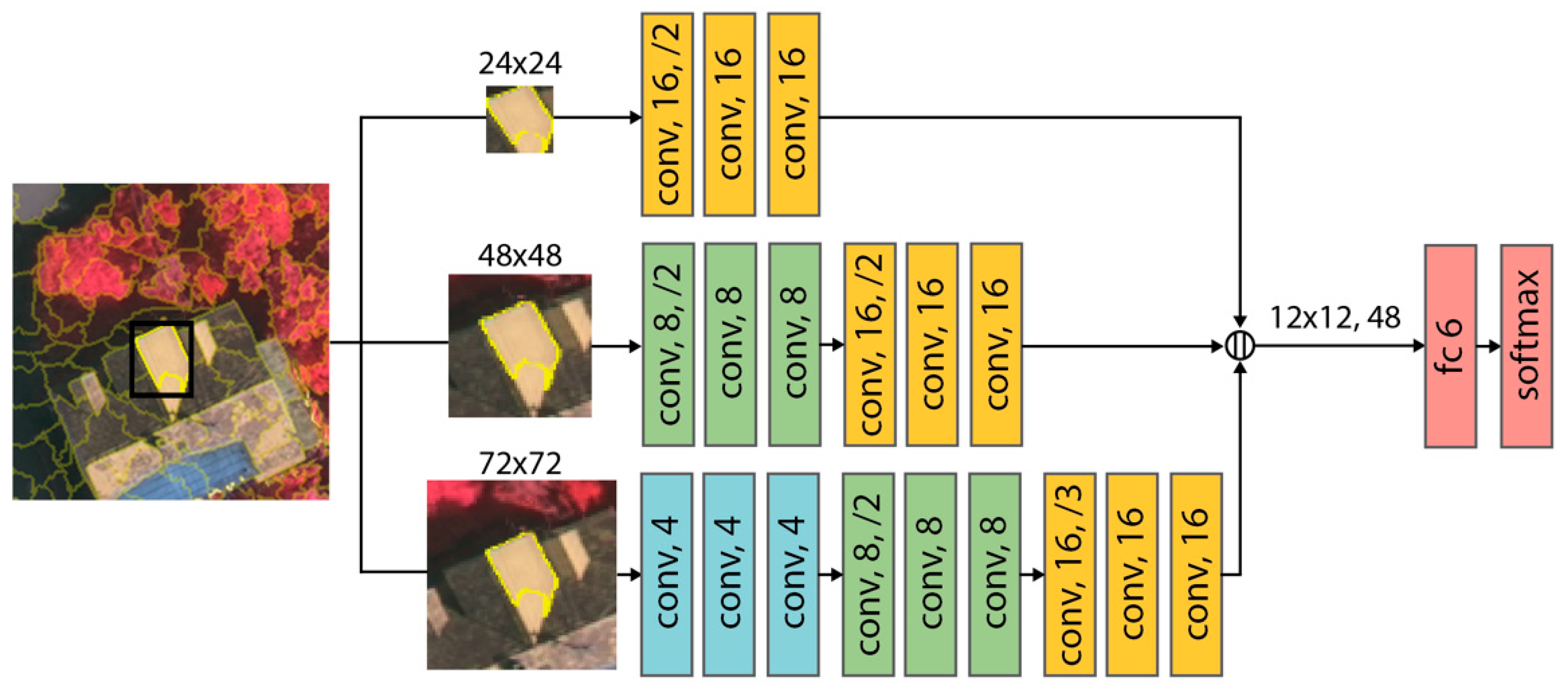
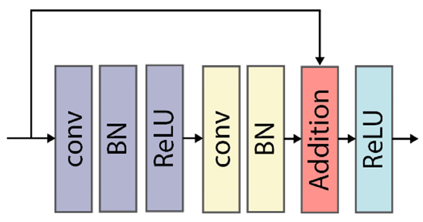
• Design a multibranch neural network structure for obtaining multiscale fusion features. Each branch is composed of residual modules with different depths that act as backbone for feature extracting.
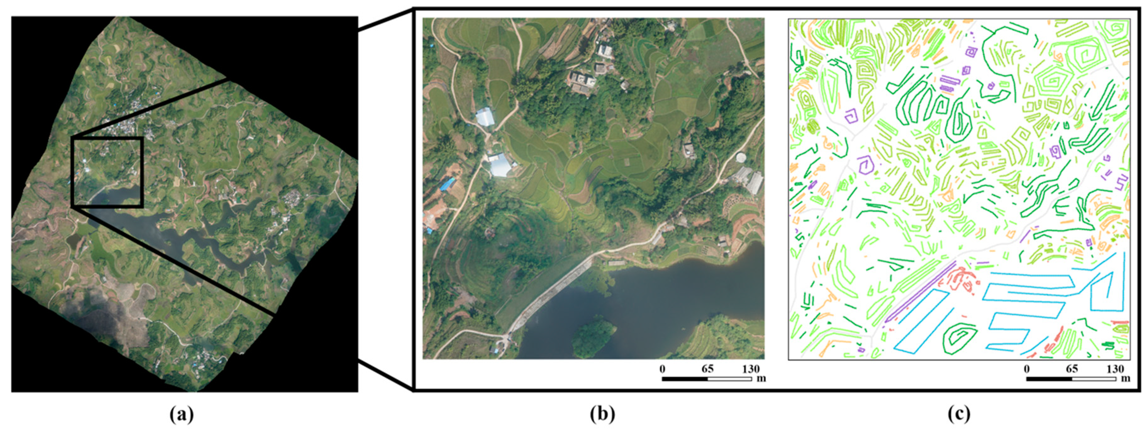
• Develop a weak labeled UAV image dataset of rural landscape for land cover classification to verify the practical feasibility of the proposed approach under various scenarios.

The proposed framework draws from established object-based methods as an auxiliary module to feed the model with objects of different scales, making the feature maps involve more contextual information contained in the limited samples. Detailed information about the multiscale input strategy and multibranch structures is introduced in the next section.

2. Methodology

The proposed approach mainly consists of three steps: (i) clustering pixels into objects for multiscale input, (ii) training a multiscale residual neural network (ResNet) for classification and then (iii) optimizing the boundaries of the classification results. To avoid large computations and reduce the salt-and-pepper effect, this study uses a clustering algorithm to obtain meaningful segments instead of traditional pixel patches as the basic computational unit (Section 2.1). Although the superpixels are homogeneous descriptions of texture, color, and other features in accordance with the visual sense, they still lack spatial relationships and semantic scene information. Therefore, by using the multiscale neighborhood information of superpixels as inputs, multiscale features of the same target superpixel are obtained for the deep neural network, which can boost the classification performance to a certain extent. This multiscale feature extraction method requires the construction of a multiscale CNN (Section 2.2). In this paper, we propose a network called a multiscale object-based network (MONet). MONet first utilizes superpixel neighborhoods at three scales as inputs. Then, it combines the feature maps obtained from three residual networks and loads them into the fully connected layer for classification. To further optimize the boundaries and reduce classification noise, this approach employs larger-scale multiresolution segmentation and a conditional random field (CRF) module for postprocessing (Section 2.3).

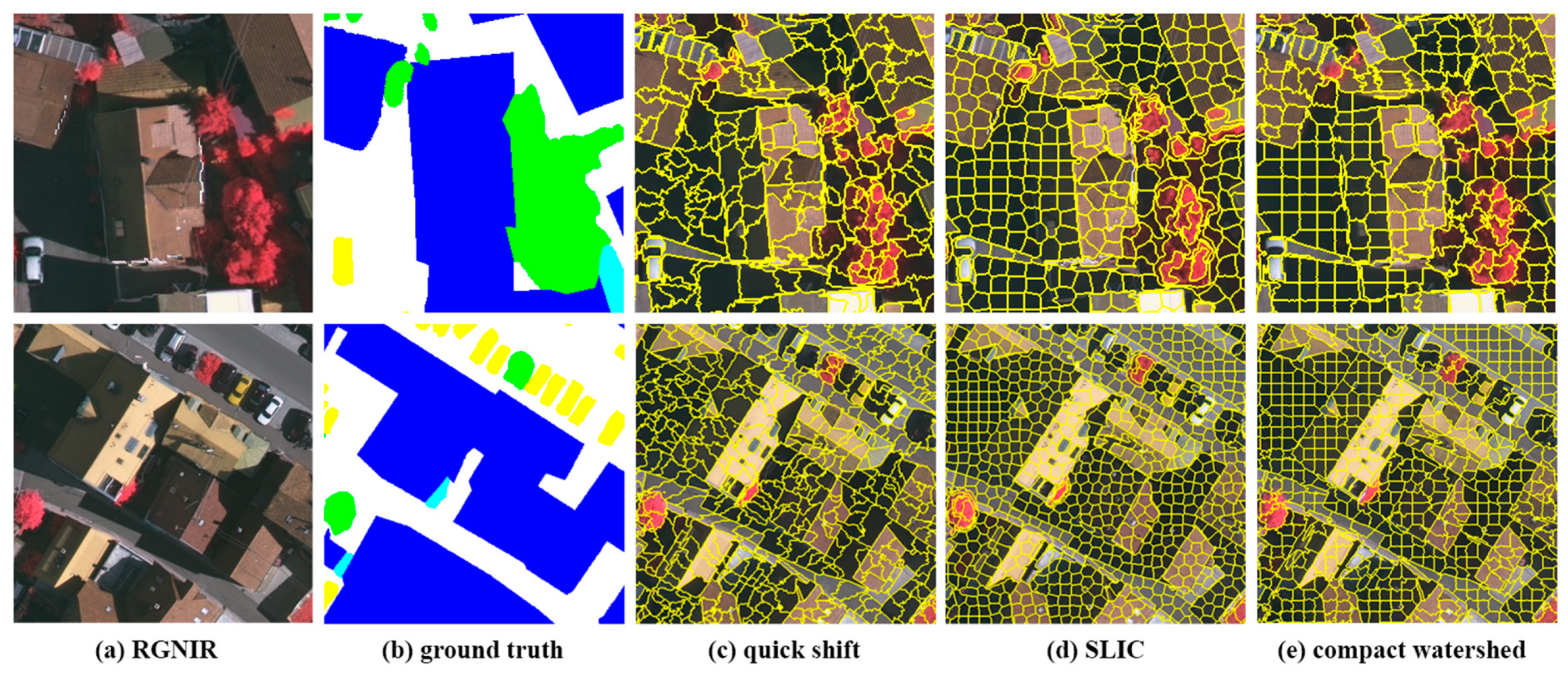
2.1. Presegmentation

Feature representation based on pixels is commonly used in traditional remote sensing image classification. In most pixel-based remote sensing image classification methods, the neighborhood of each pixel is used as the input of the network. However, the process will lead to excessive computing. For example, predicting a 1000 × 1000 pixel image requires a neighborhood of 10e6 pixels as the network input. The complexity of the method increases dramatically as the image size increases. In addition, pixelwise methods tend to obtain more detailed classification results than other methods. However, the boundaries between various objects are more broken. To resolve these issues, this paper uses feature representation based on oversegmentation, also known as superpixels. Superpixels are a group of connected pixels with similar texture, color, and brightness characteristics. There are some classical superpixel algorithms, such as quick shift, simple linear iterative clustering (SLIC) and compact watershed, which have been used in previous object-based classification studies [53,54,55]. The visualization results of the above algorithms are provided in Figure 1. In this paper, we finally select the quick shift algorithm to generate superpixels as the input of the CNN. As shown in Figure 1, for aerial image at subdecimeter resolution, the quick shift method can provide finer ground object boundaries than other methods. The segmentation results in dark areas (such as distinguishing shadows and roofs) are much better than for SLIC and compact watershed. In addition, quick shift does not need to manually set the number of segments for images of different sizes, which is beneficial for an automated classification pipeline.

Quick shift is a fast image segmentation algorithm based on an approximate kernelized mean-shift method and is a kind of local mode-seeking algorithm. It utilizes both color information (LAB color space) and image location information to compute hierarchical segmentation on multiple scales simultaneously. Specifically, the quick shift algorithm regards each pixel $\left(x,y\right)$ in the image and its d-dimensional pixel value $I\left(x,y\right)$ as a sample from a (d+2)-dimensional vector space. It then calculates the probability density estimate for each pixel (with a Gaussian kernel of standard deviation), which is defined as:

$$E\left(x,y\right)=P\left(x,y,I\left(x,y\right)\right)={\displaystyle \sum }_{x^{\prime }{y}^{\prime }}\frac{1}{{\left(2\pi \sigma \right)}^{d+2}}exp\left(-\frac{1}{2{\sigma }^2}\left[\begin{array}{c}x-x^{\prime }\\ y-y^{\prime }\\ I\left(x,y\right)-I\left(x^{\prime },y^{\prime }\right)\end{array}\right]\right)$$

(1)

Then, the quick shift algorithm constructs a tree that connects each image pixel to its nearest neighbor with a higher density value, i.e.,

$$P\left(x{}^{\prime },y{}^{\prime },I\left(x{}^{\prime },y{}^{\prime }\right)\right) > P\left(x,y,I\left(x,y\right)\right)$$

(2)

Each pixel is connected to the nearest higher-density pixel parent that achieves the minimum distance:

$$\mathrm{dist}\left(x,y\right)={\min }_{\left(x^{\prime },y^{\prime }\right)>P\left(x,y\right)}\left({\left(x-x^{\prime }\right)}^2+{\left(y-y^{\prime }\right)}^2+\Vert I\left(x,y\right)-I\left(x^{\prime },y^{\prime }\right){\Vert }_2^2\right)$$

(3)

Three main parameters influence the algorithm: the ratio, kernel size and maximum distance. The ratio is the tradeoff between the distance in the color space and the distance in the image space (larger values give more importance to color). The kernel size controls the scale of the local density approximation. The larger the size is, the larger the neighborhoods of pixels considered. The maximum distance determines the level in the hierarchical segmentation that is produced. In our experiments, these three parameters were set to 0.5, 3 and 6, respectively.

Using the similarity of pixels to divide images into nonoverlapping groups can reduce the computational complexity without sacrificing accuracy. Moreover, superpixels can better reflect the structural information and spatial topological relationships of typical ground objects. However, superpixels are homogeneous segments that contain only limited semantic information. Thus, as will be illustrated in Section 2.2, multiscale bounding boxes are used to enrich the semantic information of superpixels in practice.

2.2. Framework of MONet

VHR images contain complex objects and rich semantic information. Even objects such as cars, road signs, and chimneys in natural images can be observed in these remote sensing images. Deep neural networks are only as good as the input data, and representing the features extracted from such images through dense annotation with a dense prediction architecture is extremely time consuming and labor intensive. As mentioned in Section 1, a practical classification method for VHR images should satisfy the strong feature representation and weak labeling. When coarse labeling is inevitable, a new scheme needs to be designed to learn the comprehensive feature distributions through limited samples. The sparse sample points are augmented into meaningful objects (superpixels) through the clustering algorithm in the presegmentation stage. However, superpixels contain only the intrinsic properties of the land cover type without taking into account the contextual and distribution information. Such semantic features of the target superpixel should be learned by the model. Considering the scale issues in neighboring information and spatial relationship analysis, multiscale feature extraction and fusion are imperative: that is where MONet comes from.

The architecture of the proposed MONet model is shown in Figure 2. For each superpixel in the presegmentation stage, the neighborhoods at three scales are extracted as the network inputs. The multiscale superpixel neighborhood selection strategy used in this paper is as follows: the small-scale input is the bounding box of the target superpixel, the medium-scale input is the expanded neighborhood of the bounding box, and the large-scale input should be able to contain the 8-connected superpixels of the bounding box at least. Considering the average size of superpixels in our subdecimeter-resolution datasets, these three scales are set to 24, 48 and 72 pixels in the following experiments, respectively. The different input scales serve different purposes. The smallest input focuses on providing the intrinsic properties of the target superpixel, which is informative and specifically for feature extraction. Larger inputs involve adjacent information of the target superpixel, which enables the model to learn the spatial relation and distribution at different scales. Multiscale inputs expand the vision of object-based CNNs and enhance their feature-extracting ability when there are not enough references.

Since the multi-inputs are at three different scales, MONet consists of three corresponding and independent branches with different network depths. While avoiding overfitting, multi-depth design can lighten the whole network. Deep neural networks often suffer from the vanishing gradient problem. Similar to ResNet [56], this paper uses skip connections to address this issue. The main part of MONet is composed of many residual blocks. Each convolutional layer is followed by batch normalization (BN) and rectified linear unit (ReLU) activation layers. A skip connection connects two convolutional layers to form a residual block, as shown in Figure 3. To perform downsampling, some residual blocks contain a stride of 2 or 3. The small-scale input contains exclusive and noncontextual information, so the corresponding shallow branch contains only three residual blocks. The other two scales contain richer semantic environment information; therefore, deeper network is used (with six and nine residual blocks, respectively). The feature maps of different scales are finally downsampled so that the size of the output feature maps remains the same (i.e., 12 × 12). The network ends with a feature fusion module. The concatenated features are input into a fully connected (FC) layer with softmax for classification. In the network training process, the three network branches are trained simultaneously. After the loss is evaluated, backpropagation is performed to update the parameters of the three networks.

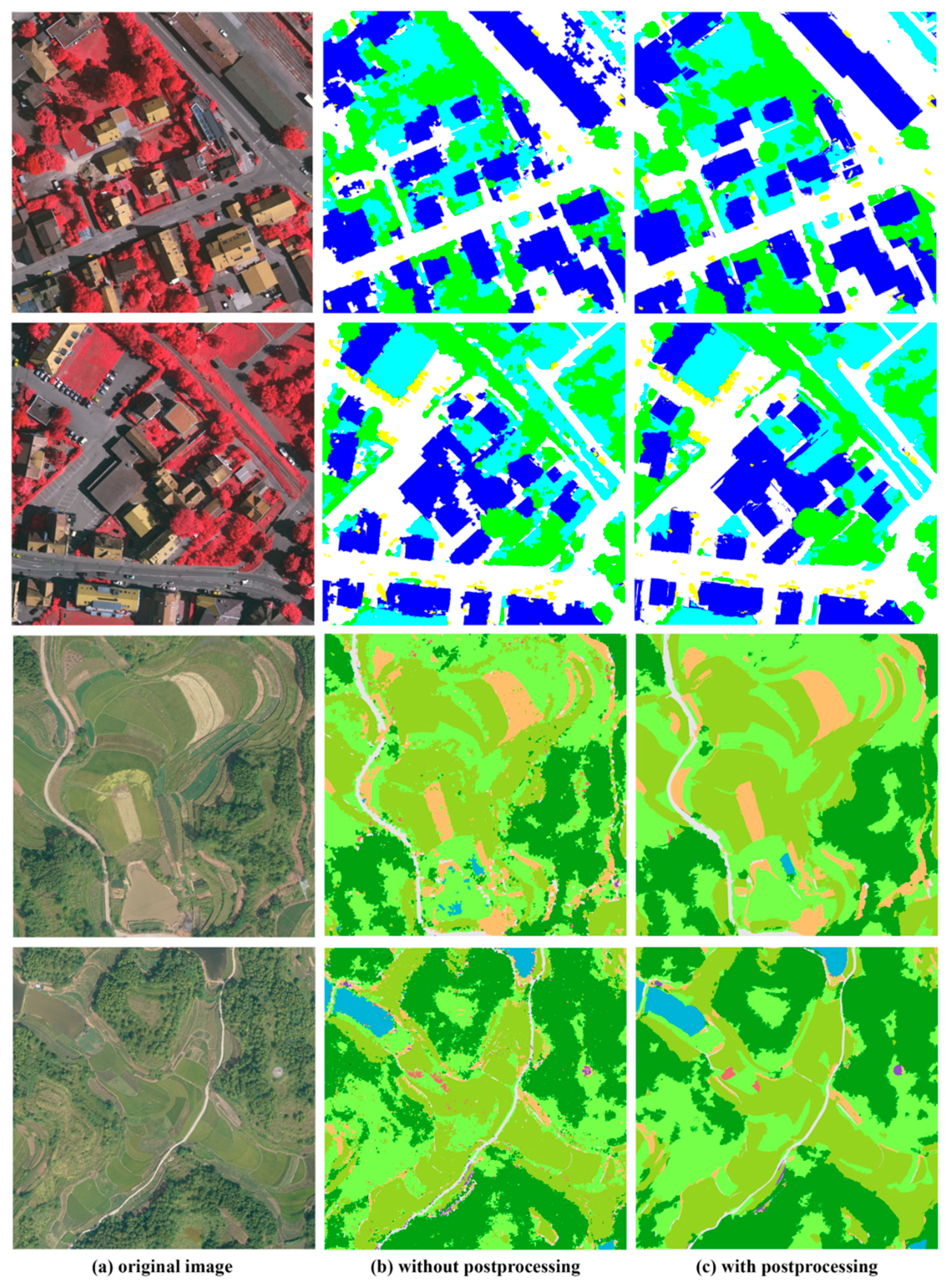
2.3. Boundary Refinement

Deeper neural networks excel at representing high-level features and can achieve state-of-the-art classification performance. However, the deep layers of the network have larger receptive fields and can yield only smooth responses. As a result, accurate location and detailed boundary information are lost. There are three commonly used ways to address the localization problem. One method is to use the image segmentation results to further constrain the boundary. Another method is to use upsampling layers combined with techniques such as skip connections to recover accurate boundary information. For example, some U-shaped convolutional networks, such as U-Net [57] and SegNet [58], achieved good accuracy using this method. The other method introduces a CRF module into the network. In this paper, we employ both image segmentation and a CRF in the boundary refinement process.

Superpixels can provide rough boundary information in the prediction and final labeling stage. However, due to the limitation of the fast clustering algorithm, this kind of boundary information cannot accurately describe the boundaries of some land cover types that are similar in color or texture. The multiresolution segmentation (MRS) algorithm is first utilized to further constrain the boundaries, especially those of large-scale objects such as buildings and roads. The MRS algorithm is based on the fractal net evolution approach (FNEA) [59] and is a bottom-up region-merging technique based on local criteria that begins with one pixel of an image object. The adjacent image objects are merged one by one in a pairwise manner to form a larger object. The underlying optimization procedure minimizes the weighted heterogeneity, which includes the color and shape heterogeneity [60]. After segmentation, a voting scheme is employed to determine the category of the object.

Then, a CRF is used to further refine the boundary. A CRF is a kind of discriminative undirected probabilistic graphical model, and it is widely used to boost models’ ability to capture fine details. Previous works employed a locally connected CRF as a postprocessing method. With the advent of DeepLab [61], a densely connected CRF [62] has almost become a standard postprocessing module for semantic segmentation. The dense CRF employs the following energy function:

$$E\left(\mathbf{x}\right)={\displaystyle \sum }_i{\psi }_i\left(x_i\right)+{\displaystyle \sum }_{i<j}{\psi }_{ij}\left(x_i, x_j\right)$$

(4)

where $\mathbf{x}$ is the set of label assignments for the pixels. The first term is the unary potential, which can be computed independently for each pixel based on the output of the network. The second term is the pairwise potential, which uses a fully connected graph to connect all the pairs of pixels in the image. It is defined as follows:

$${\psi }_{ij}\left(x_i, x_j\right)=\mu \left(x_i, x_j\right)\left[w_1\exp \left(-\frac{{\left|p_i-p_j\right|}^2}{2{\theta }_{\alpha }^2}-\frac{{\left|I_i-I_j\right|}^2}{2{\theta }_{\beta }^2}\right)+w_2\exp \left(-\frac{{\left|p_i-p_j\right|}^2}{2{\theta }_{\gamma }^2}\right)\right]$$

(5)

where $\mu$ is the label compatibility function, and $w_1$ and $w_2$ are the linear weights of the two Gaussian kernels. The first kernel is the appearance kernel, which depends on both pixel positions $p$ and the RGB color $I$. The appearance kernel ensures that nearby pixels with similar colors have the same label. The second kernel is the smoothness kernel, which removes small and isolated regions and enforces smoothness. ${\theta }_{\alpha }$, ${\theta }_{\beta }$ and ${\theta }_{\gamma }$ are hyperparameters that determine the size of the kernels. In our experiments, they were set to 60, 10 and 3, respectively.

The dense CRF performs message passing by using Gaussian filtering in the feature space, which enables the model to utilize highly efficient probabilistic inference. It takes only a few seconds to process a 5000 × 5000 pixel image and is very suitable for practical boundary refinement.

3. Experiments

In the experiments, we verify the effectiveness of the proposed MONet model. The data and experimental information are presented in Section 3.1, Section 3.2 and Section 3.3. Section 3.4 describes the comparison results based on the evaluation metrics. Further analyses and discussions of the results are provided in Section 4.

3.1. Dataset Description

To evaluate the effectiveness and generalization ability of the proposed method, the model was applied to two challenging datasets. The first dataset is the Vaihingen dataset, which is a publicly available benchmark dataset provided by the International Society for Photogrammetry and Remote Sensing (ISPRS) [7]. It consists of 38 true orthophoto (TOP) images of the town of Vaihingen in Germany and describes the typical objects in urban scenes: roads, water, buildings, cars, trees, and grass (Figure 4). The Vaihingen dataset contains 3 available channels (infrared, red and green) with a ground sampling distance of 9 cm, and each patch has a size of nearly 2500 × 2000 pixels. Note that the original dataset’s digital surface model (DSM) data and the related products are not involved in our experiments. Among these 38 TOP images, 10 TOP images with ground-truth labels were randomly selected for the experiments. The Vaihingen scene has a very high resolution that can resolve complex and challenging urban patterns, such as different sizes of cars, chimneys on roofs, and parking lots.

Most existing VHR datasets are urban scenes. To evaluate the proposed method thoroughly under various scenarios, we collected our own rural dataset at Xiangliu Reservoir (Nanning, China) using a Feima-V100 unmanned aerial vehicle equipped with a digital camera. The Xiangliu dataset has a resolution of 10 cm/pixel and contains three channels: red, blue, and green bands. The whole dataset generally contains 36 patches, and each patch is approximately 5000 × 5000 pixels (as shown in Figure 5). Among them, 11 patches, which mainly contain eight classes (i.e., floating plants, roads, crops, trees, shrubs, bare soils, buildings, and water), were randomly chosen for our experiments. Since the Xiangliu dataset does not contain a complete reference map, we labeled them manually according to careful visual interpretation and field surveying (Figure 5c). Note that only coarse labels were used here, which can be easily obtained by selecting point, line, and polygon regions of interest (ROIs) using an interaction tool. The Xiangliu dataset was collected for two reasons: (1) the dataset was used as a complement to the Vaihingen dataset. Rural scenes contain comprehensive land cover types and face the main challenges of VHR classification, especially for the detailed mapping of complex objects. For example, it is difficult to discriminate between trees and floating plants and between crops and shrubs. (2) Most semantic segmentation methods require intensive ground-truth images with accurate boundary information in the training process. However, obtaining pixel-level annotations usually requires considerable time and expensive manual work. Thus, this dataset is utilized to investigate the practicality of the proposed method for fast remote sensing image interpretation.

3.2. Training Procedure

To demonstrate the robustness of the proposed method, we randomly selected approximately 80,000 pixels from the Vaihingen dataset and selected approximately 90,000 pixels from the Xiangliu dataset as the training sample. Since the original Vaihingen dataset is class-imbalanced, a nonrepresentative model may be built. For example, the number of car samples (1.5%) is much smaller than that of other classes (roads (31.4%), water (1.1%), buildings (32.7%), trees (19.0%) and grass (14.3%)). Since cars are a class with complex structures, and we want to test the proposed method’s representativeness of high-level features, we chose a few more car samples manually. Then, 75% of the samples are selected for training, and the remaining samples are used for testing. Detailed information about the training and test samples is reported in

Table 1. Detailed information on the training and test samples from the Vaihingen dataset.

Class	Legend	Training	Test
Roads		18,856	6375
Water		595	197
Buildings		20,015	6671
Cars		3125	975
Trees		11,228	3717
Grass		8377	2797
Total	\	62,196	20,732

and

Table 2. Detailed information on the training and test samples from the Xiangliu dataset.

Class	Legend	Training	Test
Floating plants		2674	911
Roads		3779	1196
Crops		14,979	4922
Trees		14,350	4749
Shrubs		18,252	6248
Bare soil		8095	2726
Buildings		1464	454
Water		4485	1480
Total	\	68,078	22,686

.

Remote sensing image datasets with ground-truth labels are scarcer and harder to obtain than image datasets in the computer vision field. Data augmentation has become a necessity to enhance the generalization ability of neural networks and reduce overfitting. It creates transformed versions of the training images that belong to the same class as the original image. Transformations include a range of operations from the field of image manipulation, such as rotation, flipping, shifting, and zooming. Since remote sensing images are usually less variable than other images, the experiment performs only random angular rotation and flip operations on the training samples. To reduce shadow effects on the VHR images, random brightness shifting is also performed. In this way, we expand the size of the training set and the model can benefit from the artificially created variations of the samples.

The model was trained for 64 epochs with a batch size of 128. We employed the stochastic gradient optimizer Adam [63] with a learning rate of 0.001 and used learning rate reduction to prevent overfitting. More precisely, the learning rate was reduced when there was no improvement for 5 epochs. L2 regularization was used in all the convolutional layers. For batch normalization, epsilon was set to 0.001, and the momentum was set to 0.99. We used the categorical cross-entropy loss function to represent the difference between the prediction and ground-truth labels, which can be calculated as

$$-{\displaystyle \sum }_{c=1}^M{y}_{o,c}\log \left(p_{o,c}\right)$$

(6)

where $M$ is the number of possible class labels, $y_{o,c}$ is a binary indicator (0 or 1) of whether class label $c$ is the correct classification for observation $o$, and $p_{o,c}$ is the model’s predicted probability that observation $o$ is in class $c$.

The model was implemented in Python 3.7.0 using the Keras 2.2.4 deep learning library, which is a high-level neural network API written in Python. TensorFlow 1.13 [64] was utilized as a backend for the training. All the training steps and experiments ran on a machine equipped with an Intel Core i7-7800X CPU, 16 GB of RAM, and one NVIDIA GeForce RTX 2080 Ti GPU to accelerate the training process.

3.3. Evaluation Metrics

Two different metrics are employed to evaluate the classification performances: the overall accuracy (OA) and F1 score. Four combinations of predicted and true conditions are possible (

Table 3. Basic states used in computing metrics.

		True Condition
		Condition Positive	Condition Negative
Predicted condition	Predicted condition positive	TP	FP
	Predicted condition negative	FN	TN

), which are defined as true positives (TPs), true negatives (TNs), false positives (FPs) and false negatives (FNs). Then, these metrics can be calculated as below:

$$Overall Accuracy=\frac{TP+TN}{TP+TN+FP+FN}$$

(7)

$$Precision=\frac{TP}{TP+FP}$$

(8)

$$Recall=\frac{TP}{TP+FN}$$

(9)

$$F1 score=2\ast \frac{Precision\ast Recall}{Precision+Recall}$$

(10)

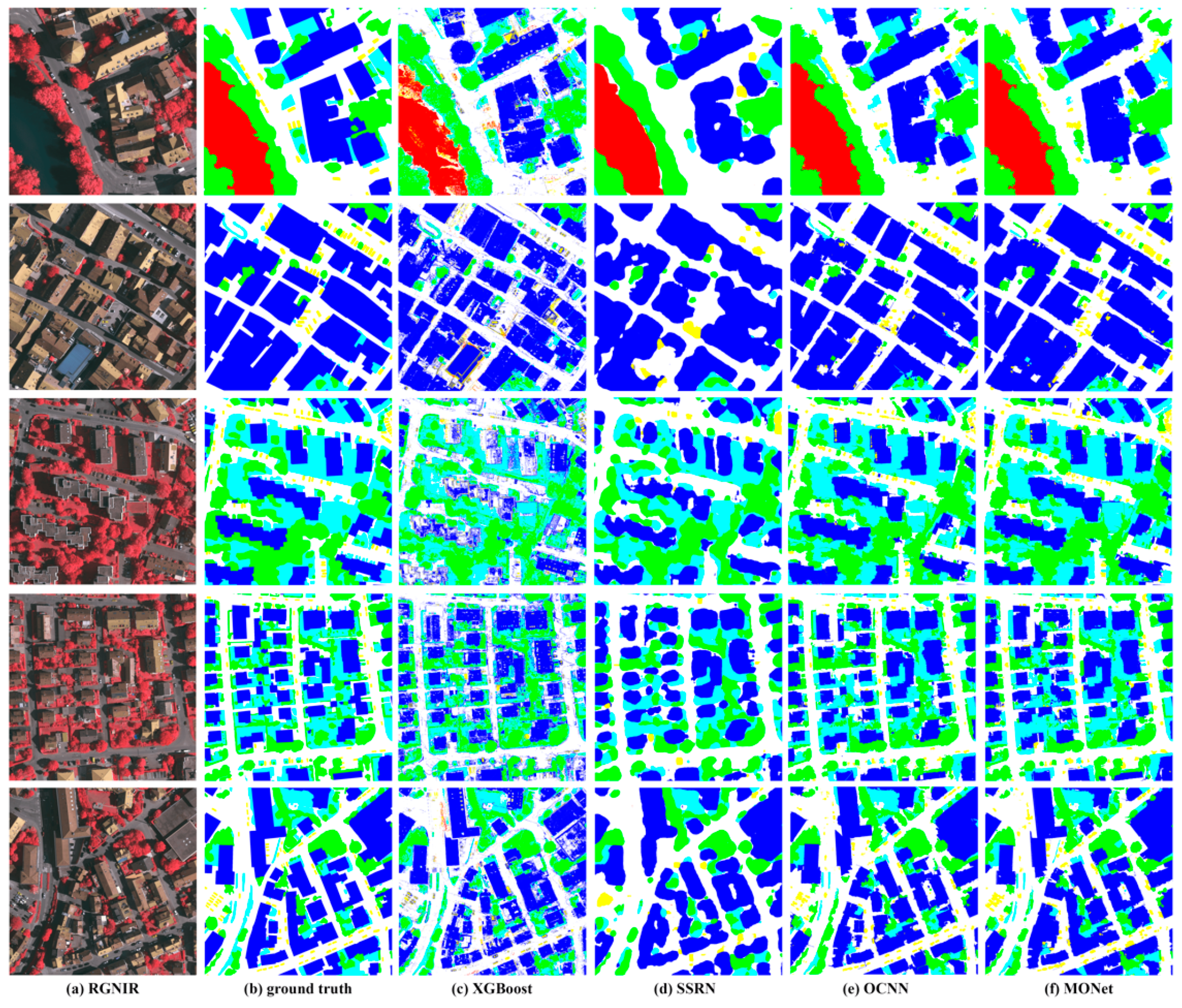
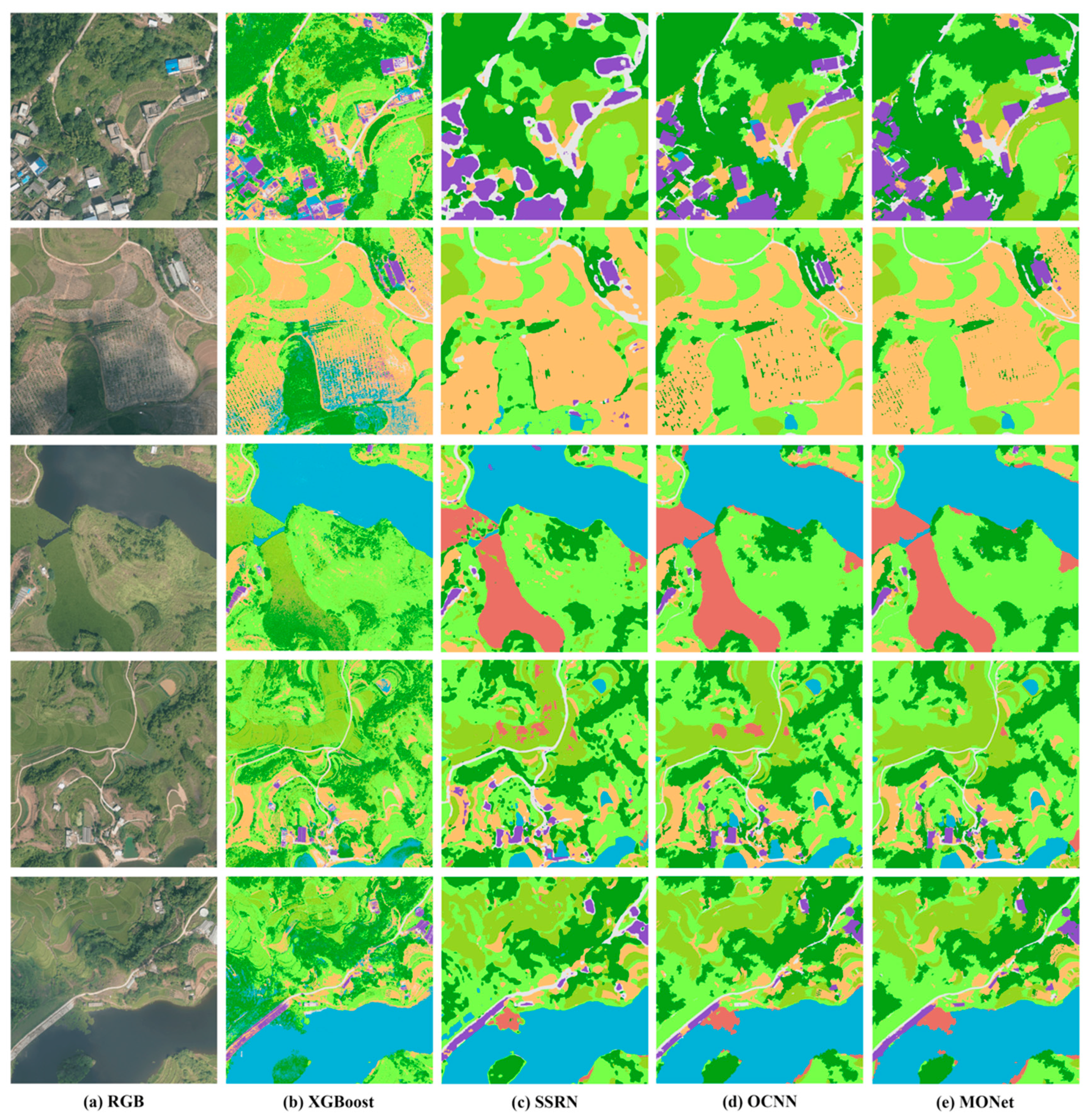
3.4. Method Comparison

We compared the MONet with other classification methods including pixel-based, patch-based CNN and object-based CNN methods by classifying all two datasets. More specifically, the comparison methods we chose were:

XGBoost [65]: This method is the most well-known decision-tree-based ensemble algorithm that utilizes a gradient boosting framework, which is trained by spectral features to predict semantic labels for aerial or satellite imagery.

Spectral-spatial residual network (SSRN) [66]: This network takes raw 3D cubes as input data and uses two spectral and two spatial residual blocks consecutively to learn discriminative features from spectral signatures and spatial contexts.

Object-based CNN (OCNN) [27]: OCNN consists of a classical AlexNet-like CNN architecture as the feature extractor and an object-based shape constraint module. The backbone is composed of 8 blocks of layers. The first 5 blocks are convolutional layers, and the last 3 blocks are fully connected layers. In between, there are some max-pooling and ReLU activation layers. Dropout and batch normalization layers are also utilized to avoid overfitting.

Three branches of MONet (denoted by MONet_1, MONet_2 and MONet_3 from the smallest scale to the largest scale): To validate the effectiveness of the multiscale strategy, three branches of MONet are extracted for comparison. Each branch involves the corresponding input size and network depth described in Section 2.2.

The selection of methods for comparison follows the principle that the selected models should be classical and reproducible. XGBoost, as an advanced machine learning algorithm, represents the pixel-based classification method; SSRN is a well performed and open-source CNN model specially designed for patch-based land cover classification; OCNN is a pioneer work in the fields of object-based CNN methods for VHR image classification. In addition, we split the multibranch structure of MONet, and each branch is added to the comparison experiment as an independent model. In this way, we verify the necessity of the multiscale strategy and the performance of residual modules with different depth in feature extraction. Note that all the methods share the same experimental parameters in our experiments, such as the batch size, number of epochs, and learning rate. The detailed quantitative and qualitative results are presented below.

Table 4. Results on the Vaihingen dataset. For each row, the highest accuracy is shown in bold.

	XGBoost	SSRN	OCNN	MONet_1	MONet_2	MONet_3	MONet
Roads	0.701	0.728	0.829	0.792	0.817	0.840	0.848
Water	0.728	0.919	0.882	0.848	0.903	0.978	0.965
Buildings	0.822	0.847	0.910	0.851	0.894	0.885	0.912
Cars	0.669	0.614	0.848	0.714	0.797	0.787	0.796
Trees	0.778	0.790	0.818	0.831	0.839	0.828	0.845
Grass	0.570	0.718	0.738	0.699	0.733	0.754	0.734
F1	0.730	0.780	0.840	0.800	0.830	0.840	0.850
OA	0.732	0.779	0.843	0.804	0.835	0.841	0.852
# of parameters	\	47,518	181,854	28,918	31,150	31,686	91,742

presents the quantitative results for XGBoost, SSRN, OCNN and MONet on the Vaihingen dataset. MONet achieves the highest OA (i.e., 85.2%) compared to other methods, and XGBoost achieves the lowest OA (i.e., 73.2%). MONet outperforms OCNN on most classes and has fewer parameters. Detailed qualitative results are shown in Figure 6.

As shown in

Table 5. Results on the Xiangliu dataset. For each row, the highest accuracy is shown in bold.

	XGBoost	SSRN	OCNN	MONet_1	MONet_2	MONet_3	MONet
Fl. plants	0.553	0.875	0.945	0.676	0.787	0.850	0.970
Roads	0.776	0.860	0.942	0.774	0.842	0.883	0.957
Crops	0.482	0.877	0.956	0.813	0.881	0.916	0.947
Trees	0.601	0.890	0.903	0.850	0.891	0.901	0.919
Shrubs	0.569	0.862	0.917	0.830	0.904	0.924	0.908
Bare soil	0.707	0.800	0.828	0.825	0.869	0.891	0.871
Buildings	0.756	0.778	0.959	0.821	0.888	0.927	0.975
Water	0.809	0.920	0.985	0.947	0.962	0.978	0.987
F1	0.610	0.870	0.920	0.830	0.890	0.910	0.930
OA	0.607	0.866	0.918	0.828	0.887	0.911	0.925
# of parameters	\	47,593	182,253	35,833	38,065	38,601	112,481

, MONet results in a better classification accuracy than the other methods on the Xiangliu dataset. MONet_3 has slightly better OA on the shrubs and bare soil classes. Figure 7 shows the comparison results in detail. To assess the practicality of the methods, their prediction times are presented in

Table 6. Experiments on prediction times (1000 × 1000 pixels, average over 10 folds).

	XGBoost	SSRN	OCNN	MONet_1	MONet_2	MONet_3	MONet
Time (s)	4.3	634.7	192.2	8.8	9.3	10.0	11.3

. Further discussion of the results can be found in Section 4.

4. Discussion

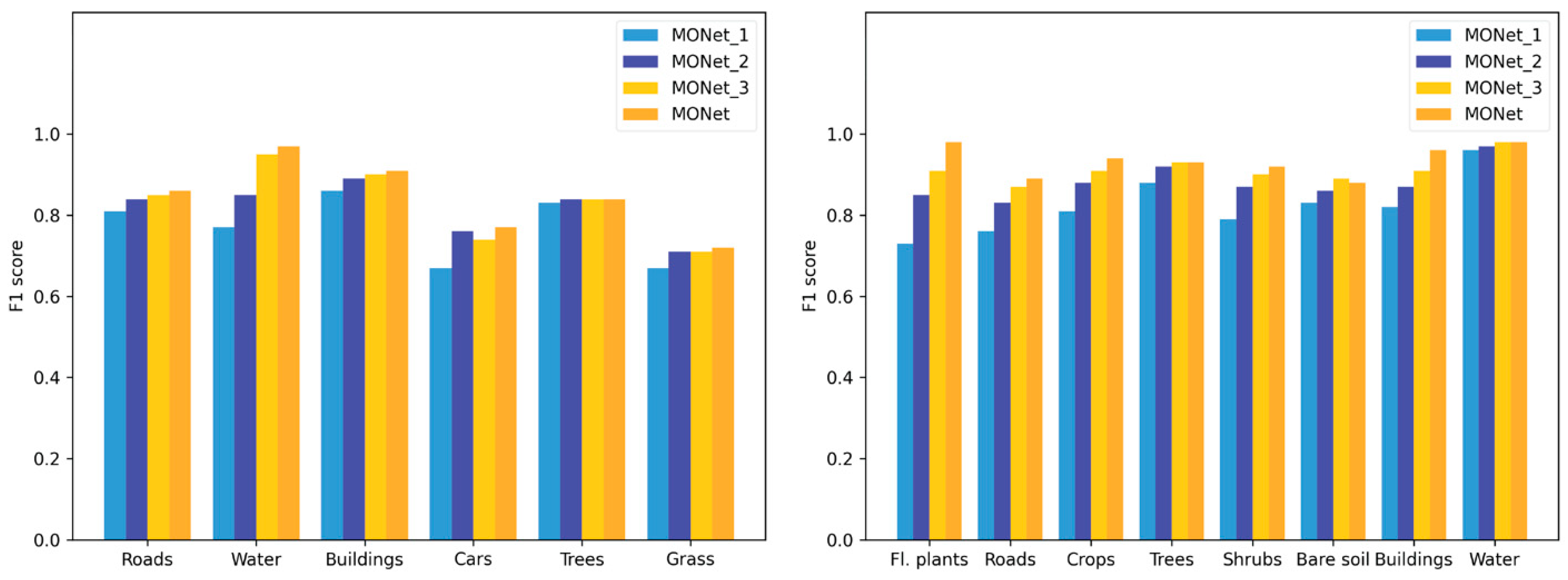
4.1. Effects of MONet and the Multiscale Strategy

Deep learning methods can avoid using handcrafted features and automatically extract more distinguishing features than traditional machine learning methods. As shown in Table 4 and Table 5, the CNN-based methods outperform XGBoost in terms of the classification accuracy. The classification maps of XGBoost show a strong salt-and-pepper phenomenon on both two datasets, which is common problem of pixelwise methods. Although the accuracies of some of the classes are not too far apart by the other methods, it cannot ensure the completeness of ground objects to achieve the intraclass consistency. Moreover, due to the lack of spectral information in the VHR images, XGBoost has no ability to distinguish the types of land covers that are easily confused visually. Categories with large spectral differences can be distinguished by pixel values alone, while similar objects or scenes require high-level features for classification. For instance, floating plants look almost the same as other plants (i.e., crops, shrubs, and trees) from above, despite their slightly different textures (Figure 7). XGBoost misclassified floating plants as trees and shrubs since it lacks the ability to extract high-level features, while the CNN-based methods can make use of contextual information when distinguishing floating plants from other plants (Figure 7).

MONet can become a deeper neural network than SSRN and OCNN by utilizing skip connections, which enhances the network’s ability to represent high-level semantic information. Given that MONet has a deeper network architecture, the top-level nodes have larger receptive fields, which makes it possible to make full use of the surrounding semantic information. It can be seen from Figure 6 that MONet performs better when distinguishing between buildings and roads than when distinguishing between other pairs of classes. Trees and grass can also be distinguished well. Similarly, the classification performances of crops, trees and shrubs are also significantly improved by MONet. In addition, MONet is more robust to changes in lighting conditions. As shown in Figure 6 and Figure 7, building shadows and cloud shadows barely have an impact on the classification results. However, for the classification of cars, OCNN outperformed MONet. Since OCNN makes predictions on each center pixel, the predictions for cars are more refined. The ground objects in the Vaihingen dataset vary across quite different scales, and the superpixels generated in the presegmentation step are relatively uniform in scale. Therefore, the classification accuracy of cars is slightly lower than that of OCNN.

The scheme of embedding a multibranch architecture in the deep learning pipeline significantly improves the feature extraction capability of the network. It can be seen from Figure 8 that as the network depth increases, the classification accuracy generally improves. It is worth mentioning that under the multiscale strategy, the discrimination accuracy of floating plants and roads in Xiangliu dataset is significantly higher than that of any single-branch model. The reason is that these two land cover types have typical spatial distribution characteristics, and the multiscale strategy can learn them more effectively. For example, the characteristic that floating plants are surrounded by water can be used as a key spatial relation to distinguish them from other plants. Similarly, the shape features of road superpixels can only be effectively represented at a certain scale. Such increases in accuracy proves the advantage of multiscale input using semantic information in the case of limited samples. While the multiscale strategy improves the classification accuracy of complex objects at different scales, simple classes such as water and bare soil can hardly benefit from the multiscale strategy. The multiscale strategy does not cause redundancy by combining networks of different depths; instead, it takes advantage of the semantic information at different scales and improves the semantically representative ability of the network.

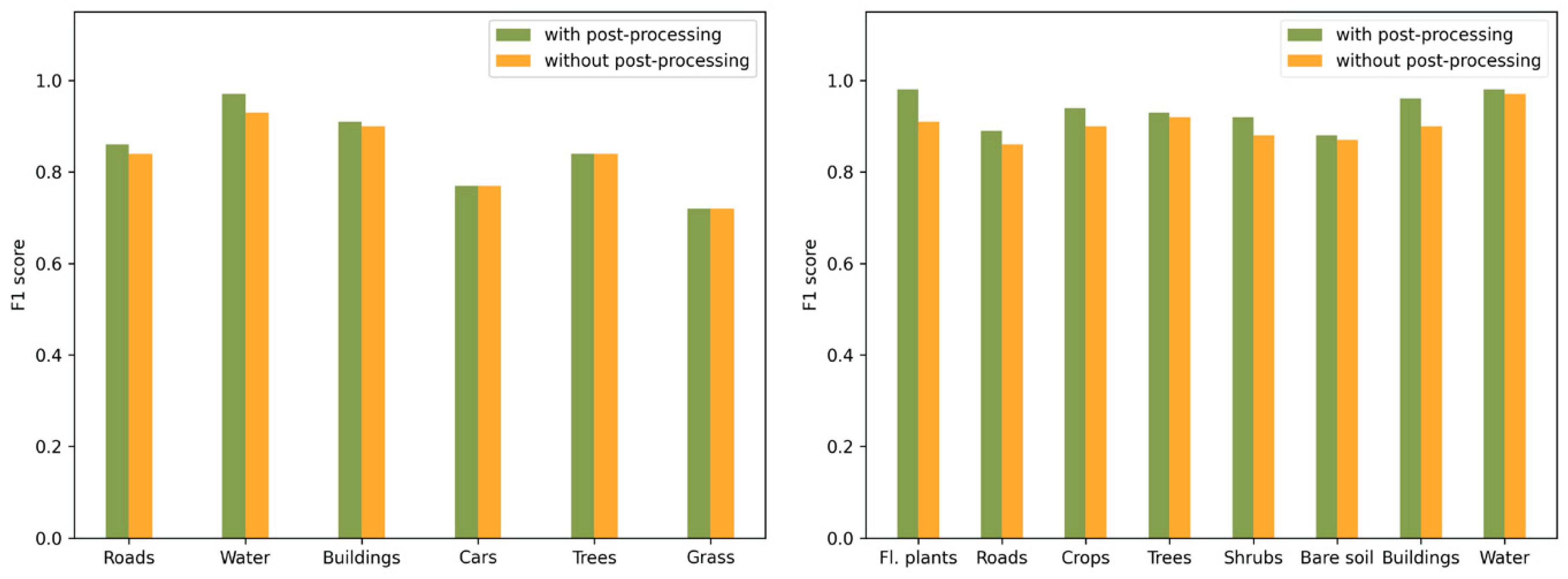
4.2. Effects of Boundary Refinement

By combining an object-oriented mechanism and a postprocessing module, the proposed framework can predict the precise contour of target objects, reduce the salt-and-pepper effect, and obtain smoother classification results. As shown in Figure 9 and Figure 10, both the qualitative and quantitative results have been improved. Parking lots, roads and roofs with similar construction materials share similar spectral properties, which makes them difficult to distinguish. Superpixels generated by the proposed method can use low-level boundary information to effectively solve this problem. In addition, MONet uses postprocessing to further optimize the boundary information.

To understand the contributions of the boundary refinement module, we compared the classification results before and after postprocessing. The postprocessing step improves the overall accuracy of classification results from 84.3% to 85.2% for the Vaihingen dataset and from 89.8% to 92.5% for the Xiangliu dataset. Obviously, for the Vaihingen dataset, postprocessing does not play a key role and only slightly improves the f1 score of buildings, water and roads (from 0.90 to 0.91, 0.93 to 0.97 and 0.84 to 0.86, respectively) because the superpixels generated in the presegmentation step have a small and relatively uniform scale, while buildings and roads are large-scale objects. Therefore, there will be inevitable loss of accuracy and boundary information. Postprocessing can be used to alleviate this problem. Although the improvement in accuracy is relatively limited, a visual assessment of the results shows that the qualitative improvement is non-negligible. Figure 10 shows that buildings are better distinguished after boundary refinement. The classification noise was reduced, and the object boundaries were strengthened, which proves the efficiency of this module. For the Xiangliu dataset, a significant improvement in the classification of most classes was achieved by postprocessing. As shown in Figure 10, roads and crops are classified into more regular segments. The classification results of trees are also smoother. The small gaps between trees are merged into an entire segment, which makes it easier for manual interpretation and thematic map production, such as vectorization and shapefile generation.

4.3. Advantages and Limitations

Combined with a deep neural network, the proposed object-oriented classification method can consider both high-level semantics and low-level geometry information. Furthermore, MONet has other practical advantages: (1) most state-of-the-art semantic segmentation approaches rely heavily on fully pixelwise annotations, which are hard to obtain in practice. MONet utilizes “lazy” labels that can be easily collected by point, line, and polygon ROI selection, which reduces the burden of manual annotations. It is more practical in the fast interpretation of remote sensing images and the thematic map production process. (2) MONet involves more parameters than traditional machine learning methods but has much fewer parameters than most semantic segmentation networks, which often involve millions of parameters to train. Therefore, the size of the training samples required by MONet will be much smaller, and the training time will be much shorter. In addition, deep learning is particularly suitable for utilizing computational hardware such as GPUs to accelerate the training process. (3) The pixel-based CNN methods receive fixed-size patches centered on each image pixel as input; then, every single pixel is predicted by the corresponding image region of the specific patch. However, the required computational power sometimes exceeds the capacity of available resources since most remote sensing images have very large file sizes. As shown in Table 6, it takes several minutes to predict a whole 1000 $\times$ 1000 pixel image, and the calculation time increases exponentially as the image size increases. The proposed object-oriented method uses superpixels as the basic unit for prediction, which requires a much shorter prediction time.

Despite all the advantages that this model can provide, our method still has some limitations, especially when the objects in the images vary across quite different scales. For example, the classification accuracy of cars by MONet is lower than that of the other methods. There are two main reasons for this phenomenon: (1) the number of car samples is much smaller than that of the other classes. (2) The sizes of the cars are very different from the size of the objects in the other classes to be classified, and it is difficult to determine a suitable segmentation scale for all the classes. That leads to another issue that has not been studied in this paper: the effects of segmentation parameters on experimental results. At this stage, the choice of segmentation parameters still stays on the interpretation of visualization results. In addition, the multiscale network used in this paper takes inputs of different sizes. More specifically, the inputs of MONet_1, MONet_2, and MONet_3 are 24 $\times$ 24, 48 $\times$ 48, and 72 $\times$ 72 pixels, respectively. In multiscale network feature fusion, different data fusion weights are not considered in our paper. Although inputs of different sizes can make full use of the semantic information surrounding superpixels, nearby superpixels are more relevant than distant ones according to the principle of spatial autocorrelation. Therefore, the size of the input data is inversely related to the relevance of the target superpixels. The larger the input scale of the data is, the smaller the proportion containing the target superpixel information, and the less it can help in the classification. The weights of the features extracted at different scales should be different. Considering the limitations of time and computing resources, adaptive multiscale weighted feature fusion will be further considered in future research so that the feature fusion process can be more meaningful and practical.

5. Conclusions

In this study, we proposed an object-oriented multiscale CNN for practical and operational VHR remote sensing image classification tasks. By combining multiscale residual networks, the method in this paper can effectively extract both low-level visual features and high-level semantic features with limited training data. To solve the problem of losing boundary information in deep neural networks, this paper employs multiresolution segmentation and a CRF for postprocessing. The results show that the method performs well on two challenging datasets and proves that it can be effectively used for VHR remote sensing image classification. In addition, the method requires only coarse-labeled training data, and the prediction process is fast, which makes it more practical for fast interpretation. However, there are still some limitations in this study. For example, for objects with large differences in scale, the classification accuracy is lower than that from other methods. In future research, the following aspects can be studied further: (1) the postprocessing steps are relatively independent of the method, so it will be better if the CRF is directly integrated into the network in an end-to-end manner; (2) different weights should be set in the feature fusion process.

References

1. Huang, B.; Zhao, B.; Song, Y. Urban Land-Use Mapping Using a Deep Convolutional Neural Network with High Spatial Resolution Multispectral Remote Sensing Imagery. Remote Sens. Environ. 2018, 214, 73–86. [Google Scholar] [CrossRef]
2. Leotta, M.J.; Long, C.; Jacquet, B.; Zins, M.; Lipsa, D.; Shan, J.; Xu, B.; Li, Z.; Zhang, X.; Chang, S.-F.; et al. Urban Semantic 3D Reconstruction From Multiview Satellite Imagery. In Proceedings of the 2019 IEEE/CVF Conference on Computer Vision and Pattern Recognition Workshops (CVPRW), Long Beach, CA, USA, 16–17 June 2019; pp. 1451–1460. [Google Scholar]
3. Liu, T.; Abd-Elrahman, A. Deep Convolutional Neural Network Training Enrichment Using Multi-View Object-Based Analysis of Unmanned Aerial Systems Imagery for Wetlands Classification. ISPRS J. Photogramm. Remote Sens. 2018, 139, 154–170. [Google Scholar] [CrossRef]
4. Colomina, I.; Molina, P. Unmanned Aerial Systems for Photogrammetry and Remote Sensing: A Review. ISPRS J. Photogramm. Remote Sens. 2014, 92, 79–97. [Google Scholar] [CrossRef] [Green Version]
5. Ban, Y.; Gong, P.; Giri, C. Global Land Cover Mapping Using Earth Observation Satellite Data: Recent Progresses and Challenges. ISPRS J. Photogramm. Remote Sens. 2015, 103, 1–6. [Google Scholar] [CrossRef] [Green Version]
6. Audebert, N.; Le Saux, B.; Lefèvre, S. Beyond RGB: Very High Resolution Urban Remote Sensing with Multimodal Deep Networks. ISPRS J. Photogramm. Remote Sens. 2018, 140, 20–32. [Google Scholar] [CrossRef] [Green Version]
7. Martins, V.S.; Kaleita, A.L.; Gelder, B.K.; da Silveira, H.L.F.; Abe, C.A. Exploring Multiscale Object-Based Convolutional Neural Network (Multi-OCNN) for Remote Sensing Image Classification at High Spatial Resolution. ISPRS J. Photogramm. Remote Sens. 2020, 168, 56–73. [Google Scholar] [CrossRef]
8. Xu, Y.; Wu, L.; Xie, Z.; Chen, Z. Building Extraction in Very High Resolution Remote Sensing Imagery Using Deep Learning and Guided Filters. Remote Sens. 2018, 10, 144. [Google Scholar] [CrossRef] [Green Version]
9. Maggiori, E.; Tarabalka, Y.; Charpiat, G.; Alliez, P. Convolutional Neural Networks for Large-Scale Remote-Sensing Image Classification. IEEE Trans. Geosci. Remote Sens. 2017, 55, 645–657. [Google Scholar] [CrossRef] [Green Version]
10. Ma, L.; Liu, Y.; Zhang, X.; Ye, Y.; Yin, G.; Johnson, B.A. Deep Learning in Remote Sensing Applications: A Meta-Analysis and Review. ISPRS J. Photogramm. Remote Sens. 2019, 152, 166–177. [Google Scholar] [CrossRef]
11. Li, M.; Zang, S.; Zhang, B.; Li, S.; Wu, C. A Review of Remote Sensing Image Classification Techniques: The Role of Spatio-Contextual Information. Eur. J. Remote Sens. 2014, 47, 389–411. [Google Scholar] [CrossRef]
12. Zou, Q.; Ni, L.; Zhang, T.; Wang, Q. Deep Learning Based Feature Selection for Remote Sensing Scene Classification. IEEE Geosci. Remote Sens. Lett. 2015, 12, 2321–2325. [Google Scholar] [CrossRef]
13. Cheng, G.; Han, J. A Survey on Object Detection in Optical Remote Sensing Images. ISPRS J. Photogramm. Remote Sens. 2016, 117, 11–28. [Google Scholar] [CrossRef] [Green Version]
14. Khatami, R.; Mountrakis, G.; Stehman, S.V. A Meta-Analysis of Remote Sensing Research on Supervised Pixel-Based Land-Cover Image Classification Processes: General Guidelines for Practitioners and Future Research. Remote Sens. Environ. 2016, 177, 89–100. [Google Scholar] [CrossRef] [Green Version]
15. Lu, D.; Weng, Q. A Survey of Image Classification Methods and Techniques for Improving Classification Performance. Int. J. Remote Sens. 2007, 28, 823–870. [Google Scholar] [CrossRef]
16. Mountrakis, G.; Im, J.; Ogole, C. Support Vector Machines in Remote Sensing: A Review. ISPRS J. Photogramm. Remote Sens. 2011, 66, 247–259. [Google Scholar] [CrossRef]
17. Belgiu, M.; Drăguţ, L. Random Forest in Remote Sensing: A Review of Applications and Future Directions. ISPRS J. Photogramm. Remote Sens. 2016, 114, 24–31. [Google Scholar] [CrossRef]
18. Ma, L.; Li, M.; Ma, X.; Cheng, L.; Du, P.; Liu, Y. A Review of Supervised Object-Based Land-Cover Image Classification. ISPRS J. Photogramm. Remote Sens. 2017, 130, 277–293. [Google Scholar] [CrossRef]
19. Blaschke, T.; Hay, G.J.; Kelly, M.; Lang, S.; Hofmann, P.; Addink, E.; Queiroz Feitosa, R.; van der Meer, F.; van der Werff, H.; van Coillie, F.; et al. Geographic Object-Based Image Analysis—Towards a New Paradigm. ISPRS J. Photogramm. Remote Sens. 2014, 87, 180–191. [Google Scholar] [CrossRef] [Green Version]
20. Hay, G.; Castilla, G. Geographic Object-Based Image Analysis (GEOBIA): A New Name for A New Discipline. In Object-Based Image Analysis—Spatial Concepts for Knowledge-Driven Remote Sensing Applications; Springer: Berlin/Heidelberg, Germany, 2008; pp. 75–89. ISBN 978-3-540-77057-2. [Google Scholar]
21. Myint, S.W.; Gober, P.; Brazel, A.; Grossman-Clarke, S.; Weng, Q. Per-Pixel vs. Object-Based Classification of Urban Land Cover Extraction Using High Spatial Resolution Imagery. Remote Sens. Environ. 2011, 115, 1145–1161. [Google Scholar] [CrossRef]
22. Duro, D.C.; Franklin, S.E.; Dubé, M.G. A Comparison of Pixel-Based and Object-Based Image Analysis with Selected Machine Learning Algorithms for the Classification of Agricultural Landscapes Using SPOT-5 HRG Imagery. Remote Sens. Environ. 2012, 118, 259–272. [Google Scholar] [CrossRef]
23. Li, M.; Ma, L.; Blaschke, T.; Cheng, L.; Tiede, D. A Systematic Comparison of Different Object-Based Classification Techniques Using High Spatial Resolution Imagery in Agricultural Environments. Int. J. Appl. Earth Obs. Geoinf. 2016, 49, 87–98. [Google Scholar] [CrossRef]
24. Tehrany, M.S.; Pradhan, B.; Jebuv, M.N. A Comparative Assessment between Object and Pixel-Based Classification Approaches for Land Use/Land Cover Mapping Using SPOT 5 Imagery. Geocarto Int. 2014, 29, 351–369. [Google Scholar] [CrossRef]
25. Arvor, D.; Durieux, L.; Andrés, S.; Laporte, M.-A. Advances in Geographic Object-Based Image Analysis with Ontologies: A Review of Main Contributions and Limitations from a Remote Sensing Perspective. ISPRS J. Photogramm. Remote Sens. 2013, 82, 125–137. [Google Scholar] [CrossRef]
26. LeCun, Y.; Bengio, Y.; Hinton, G. Deep Learning. Nature 2015, 521, 436–444. [Google Scholar] [CrossRef]
27. Zhao, W.; Du, S.; Emery, W.J. Object-Based Convolutional Neural Network for High-Resolution Imagery Classification. IEEE J. Sel. Top. Appl. Earth Obs. Remote Sens. 2017, 10, 3386–3396. [Google Scholar] [CrossRef]
28. Schmidhuber, J. Deep Learning in Neural Networks: An Overview. Neural Netw. 2015, 61, 85–117. [Google Scholar] [CrossRef] [Green Version]
29. Farabet, C.; Couprie, C.; Najman, L.; LeCun, Y. Learning Hierarchical Features for Scene Labeling. IEEE Trans. Pattern Anal. Mach. Intell. 2013, 35, 1915–1929. [Google Scholar] [CrossRef] [Green Version]
30. Chen, Y.; Lin, Z.; Zhao, X.; Wang, G.; Gu, Y. Deep Learning-Based Classification of Hyperspectral Data. IEEE J. Sel. Top. Appl. Earth Obs. Remote Sens. 2014, 7, 2094–2107. [Google Scholar] [CrossRef]
31. Ben Hamida, A.; Benoit, A.; Lambert, P.; Ben Amar, C. 3-D Deep Learning Approach for Remote Sensing Image Classification. IEEE Trans. Geosci. Remote Sens. 2018, 56, 4420–4434. [Google Scholar] [CrossRef] [Green Version]
32. Zhong, Y.; Han, X.; Zhang, L. Multi-Class Geospatial Object Detection Based on a Position-Sensitive Balancing Framework for High Spatial Resolution Remote Sensing Imagery. ISPRS J. Photogramm. Remote Sens. 2018, 138, 281–294. [Google Scholar] [CrossRef]
33. Zhang, C.; Yue, P.; Tapete, D.; Jiang, L.; Shangguan, B.; Huang, L.; Liu, G. A Deeply Supervised Image Fusion Network for Change Detection in High Resolution Bi-Temporal Remote Sensing Images. ISPRS J. Photogramm. Remote Sens. 2020, 166, 183–200. [Google Scholar] [CrossRef]
34. Ji, S.; Shen, Y.; Lu, M.; Zhang, Y. Building Instance Change Detection from Large-Scale Aerial Images Using Convolutional Neural Networks and Simulated Samples. Remote Sens. 2019, 11, 1343. [Google Scholar] [CrossRef] [Green Version]
35. Bejiga, M.B.; Melgani, F. Gan-Based Domain Adaptation for Object Classification. In Proceedings of the IGARSS 2018—2018 IEEE International Geoscience and Remote Sensing Symposium, Valencia, Spain, 22–27 July 2018; pp. 1264–1267. [Google Scholar]
36. Zhang, S.; Wu, R.; Xu, K.; Wang, J.; Sun, W. R-CNN-Based Ship Detection from High Resolution Remote Sensing Imagery. Remote Sens. 2019, 11, 631. [Google Scholar] [CrossRef] [Green Version]
37. Xu, S.; Mu, X.; Chai, D.; Zhang, X. Remote Sensing Image Scene Classification Based on Generative Adversarial Networks. Remote Sens. Lett. 2018, 9, 617–626. [Google Scholar] [CrossRef]
38. Zhu, X.X.; Tuia, D.; Mou, L.; Xia, G.-S.; Zhang, L.; Xu, F.; Fraundorfer, F. Deep Learning in Remote Sensing: A Comprehensive Review and List of Resources. IEEE Geosci. Remote Sens. Mag. 2017, 5, 8–36. [Google Scholar] [CrossRef] [Green Version]
39. Tuia, D.; Flamary, R.; Courty, N. Multiclass Feature Learning for Hyperspectral Image Classification: Sparse and Hierarchical Solutions. ISPRS J. Photogramm. Remote Sens. 2015, 105, 272–285. [Google Scholar] [CrossRef] [Green Version]
40. Sharma, A.; Liu, X.; Yang, X.; Shi, D. A Patch-Based Convolutional Neural Network for Remote Sensing Image Classification. Neural Netw. 2017, 95, 19–28. [Google Scholar] [CrossRef]
41. Zhao, W.; Du, S. Learning Multiscale and Deep Representations for Classifying Remotely Sensed Imagery. ISPRS J. Photogramm. Remote Sens. 2016, 113, 155–165. [Google Scholar] [CrossRef]
42. Li, P.; Ren, P.; Zhang, X.; Wang, Q.; Zhu, X.; Wang, L. Region-Wise Deep Feature Representation for Remote Sensing Images. Remote Sens. 2018, 10, 871. [Google Scholar] [CrossRef] [Green Version]
43. Zhao, W.; Du, S.; Wang, Q.; Emery, W.J. Contextually Guided Very-High-Resolution Imagery Classification with Semantic Segments. ISPRS J. Photogramm. Remote Sens. 2017, 132, 48–60. [Google Scholar] [CrossRef]
44. Papadomanolaki, M.; Vakalopoulou, M.; Karantzalos, K. A Novel Object-Based Deep Learning Framework for Semantic Segmentation of Very High-Resolution Remote Sensing Data: Comparison with Convolutional and Fully Convolutional Networks. Remote Sens. 2019, 11, 684. [Google Scholar] [CrossRef] [Green Version]
45. Audebert, N.; Saux, B.L.; Lefèvre, S. Semantic Segmentation of Earth Observation Data Using Multimodal and Multi-Scale Deep Networks. arXiv 2016, arXiv:1609.06846. [Google Scholar]
46. Li, W.; He, C.; Fang, J.; Zheng, J.; Fu, H.; Yu, L. Semantic Segmentation-Based Building Footprint Extraction Using Very High-Resolution Satellite Images and Multi-Source GIS Data. Remote Sens. 2019, 11, 403. [Google Scholar] [CrossRef] [Green Version]
47. Ghazouani, F.; Farah, I.R.; Solaiman, B. Semantic Remote Sensing Scenes Interpretation. In Ontology in Information Science; Thomas, C., Ed.; InTech: London, UK, 2018; ISBN 978-953-51-3887-7. [Google Scholar]
48. Huang, B.; Lu, K.; Audeberr, N.; Khalel, A.; Tarabalka, Y.; Malof, J.; Boulch, A.; Le Saux, B.; Collins, L.; Bradbury, K.; et al. Large-Scale Semantic Classification: Outcome of the First Year of Inria Aerial Image Labeling Benchmark. In Proceedings of the IGARSS 2018—2018 IEEE International Geoscience and Remote Sensing Symposium, Valencia, Spain, 22–27 July 2018; pp. 6947–6950. [Google Scholar]
49. Yao, X.; Han, J.; Cheng, G.; Qian, X.; Guo, L. Semantic Annotation of High-Resolution Satellite Images via Weakly Supervised Learning. IEEE Trans. Geosci. Remote Sens. 2016, 54, 3660–3671. [Google Scholar] [CrossRef]
50. Liu, Y.; Piramanayagam, S.; Monteiro, S.T.; Saber, E. Dense Semantic Labeling of Very-High-Resolution Aerial Imagery and LiDAR with Fully-Convolutional Neural Networks and Higher-Order CRFs. In Proceedings of the 2017 IEEE Conference on Computer Vision and Pattern Recognition Workshops (CVPRW), Honolulu, HI, USA, 21–26 July 2017; pp. 1561–1570. [Google Scholar]
51. Yang, Z.; Jiang, W.; Xu, B.; Zhu, Q.; Jiang, S.; Huang, W. A Convolutional Neural Network-Based 3D Semantic Labeling Method for ALS Point Clouds. Remote Sens. 2017, 9, 936. [Google Scholar] [CrossRef] [Green Version]
52. Lateef, F.; Ruichek, Y. Survey on Semantic Segmentation Using Deep Learning Techniques. Neurocomputing 2019, 338, 321–348. [Google Scholar] [CrossRef]
53. Vedaldi, A.; Soatto, S. Quick Shift and Kernel Methods for Mode Seeking. In Proceedings of the Computer Vision—ECCV 2008, Marseille, France, 12–18 October 2008; Forsyth, D., Torr, P., Zisserman, A., Eds.; Springer: Berlin/Heidelberg, Germany, 2008; pp. 705–718. [Google Scholar]
54. Achanta, R.; Shaji, A.; Smith, K.; Lucchi, A.; Fua, P.; Süsstrunk, S. SLIC Superpixels Compared to State-of-the-Art Superpixel Methods. IEEE Trans. Pattern Anal. Mach. Intell. 2012, 34, 2274–2282. [Google Scholar] [CrossRef] [Green Version]
55. Neubert, P.; Protzel, P. Compact Watershed and Preemptive SLIC: On Improving Trade-offs of Superpixel Segmentation Algorithms. In Proceedings of the 2014 22nd International Conference on Pattern Recognition (ICPR 2014), Stockholm, Sweden, 24–28 August 2014; pp. 996–1001. [Google Scholar]
56. He, K.; Zhang, X.; Ren, S.; Sun, J. Deep Residual Learning for Image Recognition. In Proceedings of the 2016 IEEE Conference on Computer Vision and Pattern Recognition (CVPR), Las Vegas, NV, USA, 27–30 June 2016; pp. 770–778. [Google Scholar]
57. Ronneberger, O.; Fischer, P.; Brox, T. U-Net: Convolutional Networks for Biomedical Image Segmentation; Springer: Cham, Switzerland, 2015; Volume 9351, p. 241. ISBN 978-3-319-24573-7. [Google Scholar]
58. Badrinarayanan, V.; Kendall, A.; Cipolla, R. SegNet: A Deep Convolutional Encoder-Decoder Architecture for Image Segmentation. IEEE Trans. Pattern Anal. Mach. Intell. 2017, 39, 2481–2495. [Google Scholar] [CrossRef]
59. Baatz, M.; Schäpe, A. Multiresolution Segmentation: An Optimization Approach for High Quality Multi-Scale Image Segmentation. J. Geosci. Geomat. 2018, 6, 103–123. [Google Scholar]
60. Gao, H.; Tang, Y.; Jing, L.; Li, H.; Ding, H. A Novel Unsupervised Segmentation Quality Evaluation Method for Remote Sensing Images. Sensors 2017, 17, 2427. [Google Scholar] [CrossRef]
61. Chen, L.-C.; Papandreou, G.; Kokkinos, I.; Murphy, K.; Yuille, A.L. DeepLab: Semantic Image Segmentation with Deep Convolutional Nets, Atrous Convolution, and Fully Connected CRFs. IEEE Trans. Pattern Anal. Mach. Intell. 2018, 40, 834–848. [Google Scholar] [CrossRef] [PubMed]
62. Krähenbühl, P.; Koltun, V. Efficient Inference in Fully Connected CRFs with Gaussian Edge Potentials. arXiv 2012, arXiv:1210.5644. [Google Scholar]
63. Kingma, D.; Ba, J. Adam: A Method for Stochastic Optimization. In Proceedings of the International Conference on Learning Representations, Banff, AB, Canada, 14–16 April 2014. [Google Scholar]
64. Abadi, M.; Agarwal, A.; Barham, P.; Brevdo, E.; Chen, Z.; Citro, C.; Corrado, G.S.; Davis, A.; Dean, J.; Devin, M.; et al. TensorFlow: Large-Scale Machine Learning on Heterogeneous Distributed Systems. arXiv 2016, arXiv:1603.04467. [Google Scholar]
65. Chen, T.; Guestrin, C. XGBoost: A Scalable Tree Boosting System. In Proceedings of the 22nd Acm Sigkdd International Conference on Knowledge Discovery and Data Mining, San Francisco, CA, USA, 13–17 August 2016; p. 794. [Google Scholar]
66. Zhong, Z.; Li, J.; Luo, Z.; Chapman, M. Spectral–Spatial Residual Network for Hyperspectral Image Classification: A 3-D Deep Learning Framework. IEEE Trans. Geosci. Remote Sens. 2018, 56, 847–858. [Google Scholar] [CrossRef]
Figure 1. Examples of superpixel segmentation: column (a) original images; column (b) ground truth maps; column (ce) superpixel segmentation results of the quick shift, simple linear iterative clustering (SLIC), and compact watershed, respectively.
Remotesensing 13 00364 g001
Figure 2. The architecture of multiscale object-based network (MONet). Each conv block represents a residual block (see Figure 3), and the number refers to the number of feature map channels. The /2 or /3 indicates the downsampling stride.
Remotesensing 13 00364 g002
Figure 3. Illustration of a residual block. This block includes two convolutional layers, and a skip connection directly adds the input to the output.
Remotesensing 13 00364 g003
Figure 4. The Vaihingen dataset and its reference map. (a) Overview of the Vaihingen dataset, (b) the whole image of one patch, and (c) the corresponding reference map.
Remotesensing 13 00364 g004
Figure 5. The Xiangliu dataset and its reference map. (a) Overview of the Xiangliu dataset, (b) the whole image of one patch, and (c) the corresponding reference map.
Remotesensing 13 00364 g005
Figure 6. Results on the Vaihingen dataset: column (a) original images; column (b) ground truth maps; column (cf) results of XGBoost, SSRN, OCNN and MONet methods, respectively.
Remotesensing 13 00364 g006
Figure 7. Results on the Xiangliu dataset: column (a) original images; column (be) results of XGBoost, SSRN, OCNN and MONet methods, respectively.
Remotesensing 13 00364 g007
Figure 8. Experiments on the multiscale strategy for the Vaihingen (left) and Xiangliu (right) datasets.
Remotesensing 13 00364 g008
Figure 9. Quantitative experiments on postprocessing for the Vaihingen (left) and Xiangliu (right) datasets.
Remotesensing 13 00364 g009
Figure 10. Qualitative experiments on postprocessing: column (a) original VHR images from Vaihingen dataset and Xiangliu dataset; column (b) results without postprocessing and column; column (c) results with postprocessing.
Remotesensing 13 00364 g010