
Forest Road Detection Using LiDAR Data and Hybrid Classification
by
 , , and
Sandra Buján
1,*,† ,
,
Juan Guerra-Hernández
2,3,† ,
,
Eduardo González-Ferreiro
4,† and
and
David Miranda
1,† 1
GI-1934 TB—LaboraTe, Departamento de Ingeniería Agroforestal and IBADER, Universidade de Santiago de Compostela, Escola Politécnica Superior de Ingeniería, Campus de Lugo, 27002 Lugo, Spain
2
3edata, Centro de Iniciativas Empresariais, Fundación CEL, O Palomar s/n, 27004 Lugo, Spain
3
Forest Research Centre, School of Agriculture, University of Lisbon, Instituto Superior de Agronomia (ISA), Tapada da Ajuda, 1349-017 Lisboa, Portugal
4
GI-202-GEOINCA, Departamento de Tecnología Minera, Topografía y de Estructuras, Universidad de León, Av. Astorga, 15, 24401 Ponferrada, Spain
*
Author to whom correspondence should be addressed.
†
These authors contributed equally to this work.
Remote Sens. 2021, 13(3), 393; https://0-doi-org.brum.beds.ac.uk/10.3390/rs13030393
Submission received: 23 December 2020
/
Revised: 15 January 2021
/
Accepted: 18 January 2021
/
Published: 23 January 2021
(This article belongs to the Special Issue 3D Point Clouds in Forest Remote Sensing)
Abstract
:Knowledge about forest road networks is essential for sustainable forest management and fire management. The aim of this study was to assess the accuracy of a new hierarchical-hybrid classification tool (HyClass) for mapping paved and unpaved forest roads with LiDAR data. Bare-earth and low-lying vegetation were also identified. For this purpose, a rural landscape (area 70 ha) in northwestern Spain was selected for study, and a road network map was extracted from the cadastral maps as the ground truth data. The HyClass tool is based on a decision tree which integrates segmentation processes at local scale with decision rules. The proposed approach yielded an overall accuracy (OA) of 96.5%, with a confidence interval (CI) of 94.0–97.6%, representing an improvement over pixel-based classification (OA = 87.0%, CI = 83.7–89.8%) using Random Forest (RF). In addition, with the HyClass tool, the classification precision varied significantly after reducing the original point density from 8.7 to 1 point/m. The proposed method can provide accurate road mapping to support forest management as an alternative to pixel-based RF classification when the LiDAR point density is higher than 1 point/m.
1. Introduction
1.1. Background
The focus of forest policy and management in Europe has shifted from wood production to sustainable ecosystem management [1]. Sustainable forest management should enhance all goods and services provided by forests, by considering the multifunctional role of forests and forest resources, including provision of, e.g., timber and non-timber products (fruits, resins, mushrooms, etc.), watershed regulation and water supply, grazing by livestock, climate regulation, hunting, fishing and outdoor recreation. In this respect, forest roads have become vital components of the human use of forest systems throughout history, providing access that enables people to study, enjoy, contemplate or extract forest resources [2].
Forest road networks provide connections to primary road networks and also between different forested areas [3]. In Spain, most forest road networks are designed to enable selvicultural and timber extraction, although they are also essential for forest risk management, serving as preventive infrastructures (fire breaks), providing access for wildfire forest surveillance and fire prevention and suppression activities and acting as deterrents for illegal activities (e.g., arson, poaching or illegal logging and fruit collection). From the ecological point of view, forest roads are often considered ecosystems themselves (e.g., [4]), and their presence in forests may provide benefits (e.g., as edge habitats and connection between core habitats) and/or drawbacks (e.g., debris and sliding sediments, habitat fragmentation, wildlife disturbance and traffic accidents, corridors for exotic species and pathogens, loss of water quality and waste dumping).
Detailed maps of forest roads are essential for timely and improved sustainable forest management [3]. Land and forest managers need high-quality up-to-date information about forest roads in order to balance the benefits, problems and risks, both for society and forests, to enable them to make the best management decisions based on the purpose of the road and its effects [2], including usage time and persistence, number of roads and layout, width and surface characteristics (paved or unpaved) and maintenance needs.
In Spain, forest roads are often digitized by photo-interpretation for forest management activities, which involve low efficiency and time-consuming processes. In Spain, the PNOA project (Plan Nacional de Ortografía Aérea) is the primary source of information for delineating forest roads. Since 2004, the PNOA has provided photogrammetric products with a periodic cover of 2–3 years for the whole of Spain, with a spatial resolution of 0.25 m and RGB and NIR bands. Therefore, information about forest roads is frequently outdated as a result of the arduous processes involved in collecting data (especially in NW Spain where the presence of fast-growing forest species implies more intensive forestry activity, with a high rate of road construction associated with logging activities). Information is also often incomplete due to difficulties in photo-interpretation of complex forest areas (as information about the type of surface, the road width, the maintenance level and its connectivity is often lacking).
The positioning accuracy of existing data on forest roads is very variable (as it strongly depends on the expertise of the digitizer), with missing outlines (especially in those areas with underneath narrow forest roads and paths below dense forest canopies), and added difficulties in open areas (e.g., poorly maintained wide firebreaks, which are rapidly colonized by heliophilous shrub species, creating a continuous cover that often hinders the edge detection). For all of these reasons, it is essential to develop automatic reliable processes for identifying and mapping forest roads. Such methods should be simple, inexpensive and upgradeable.
1.2. Brief Review of the State-of-Art
Most efforts focused on developing methods of detecting roads have tried to respond to the needs of both urban planning/management and sustainable forest management, resulting in increased research output in these fields. Despite the importance of these subjects, most studies concern the detection of paved roads in urban or peri-urban areas. In addition, although this is a very active field of research, which tends towards the total automation of all processes, manual editing is still used, mainly at the post-processing stage [5]. Current methods are designed to address, mitigate or, at best, solve challenges involving the identification of roads. In this respect, the discontinuities of roads (omission errors) and the spectral similarity between categories (commission errors) are the major challenges. The main causes of the discontinuities are: (1) the presence of non-ground objects, such as vehicles, which cause errors in the Digital Terrain Models (DTM) [6], or buildings, which shade the roads [7]; (2) roads covered by trees, which cause interference in GPS signals [8], lack of information when using images [5] or reduction of number of points when using LiDAR data [9]; (3) wrongly identified relationship between the road characteristics and the spatial resolution of the data; and (4) steep relief, which causes filtering errors at the road edges [10]. Moreover, the spectral confusion between land cover types is a major cause of commission errors (e.g., flat areas and no tree vegetation, where the cover adjacent to roads and the roads themselves are similar, such as bare-earth and dirt roads).
Although the previous cases can be found in any environment, those related to non-ground objects (Cause 1) are characteristic of urban/peri-urban areas, while others, such as road covered by trees or steep relief (Cause 2), are more common in rural and forest areas. For example, tall buildings in urban environments often produce occlusions or shadows on the data, and, although unequal in consequence, these errors occur in both aerial/satellite images and LiDAR point clouds [6,11]. The presence of vehicles, which may cause errors in the DTM or increase the number of gaps in the extracted-road network (due to their size and height) is also usual in such areas [6]. However, it is not usual to find either occlusion errors in road classification (due to the dense vegetation) or DTM errors caused by steep slope, as in rural and forested areas [3]. This may be one reason why the methods of road detection that are used in urban areas are not applied in rural areas, and vice versa, or for identification of non-paved roads. Together with the fact that most of the methods developed are used in urban areas, this results in a net deficit of methods than can be used to address the needs of rural areas [12]. In addition, despite the obvious impact of aforementioned challenges on the quality of the extracted roads, studies explicitly analyzing this aspect are scarce [3].
Three levels of automation exist: manual, automatic and semi-automatic (which combines automatic processes and manual editing) (Figure 1). The first group includes traditional methods based on surveying techniques or GPS to capture spatial data [8] as well as photointerpretation and manual digitization of roads (which use aerial/satellite images or the LiDAR-derived layers) [13]. Although these techniques are the most accurate and robust, they are also time-consuming and costly [14]. This group also includes participatory GIS; in a recent great study, a mobile application, RoadLab Pro, was used to automatically map the driving location of six different drivers [12]. The data were collected by taking advantage of the car/truck journeys by users working for organizations operating in the study area. In this particular case, the data collection was limited to areas transited by vehicles, and narrow roads or abandoned logging roads were excluded. Assuming no technical limitations for users travelling on foot, this is an easy method of collecting data, although less accurate than traditional methods and possibly more expensive than in the case reported [12].
Data collected using manual techniques are usually used to train semi-automatic and automatic methods and assess the accuracy of the detection. Despite the large number of automatic methods for identifying roads, examples of applications in rural areas are scarce. Passive sensors, which are widely used in urban areas, are not efficient in highly vegetated areas such as rural environments [15]. Because of this limitation, LiDAR technology is considered the best option for detecting roads in forest areas, owing to its ability to provide data on the area below canopy cover. Studies which have used these data in raster format have mainly considered three variables: nDSM, ground slope and LiDAR intensity [3,5,6]. However, a much larger number of variables can be obtained from the LiDAR point clouds (e.g., [16,17]). Within the field of road detection and mapping, no studies have yet explored the potential of these data beyond consideration of the aforementioned variables. This type of analysis could provide a useful basis for identifying variables not yet considered and for assessing the possibility of developing double-aptitude methods (urban–rural/paved–unpaved).
A wide variety of automatic methods can be used to detect roads, and there are also many ways to group them (see review by Wang et al. [18] or Tejenaki et al. [6]); however, examples of unpaved road identification in rural areas are scarce [5,19]. Considering the unit of analysis and taking into account that the data are in raster form, some methods use the pixel as the basic unit of analysis [3,20]. However, the improvement in spatial resolution leads to an increase in the spectral heterogeneity of the cover. Moreover, several pixels are needed to define an object. These limitations, together with the development of sophisticated and efficient processing tools, have led to a paradigm shift. Thus, the possibility of using spatial patterns arose as complementary to object-based methods, in which the basic unit of analysis is the object, which comprises a continuous region of pixels with homogeneous values. Segmentation, the process where by such objects are delimited, enables a reduction in the internal variability of the cover as well as elimination of the salt and pepper effect, which is typical of pixel-based classifications. It also enables the use of spatial, morphological or context variables as well as spectral variables. Although the segmentation improves the results of pixel-based methods, it also plays the role of executioner, because it is responsible for most of the erroneous assignations and the occurrence of mixed objects (over and under segmentation) [21].
Some studies have shown that object-based classification produces better results than the pixel-based methods on a global scale (study area). Nonetheless, if the results are analyzed on a class scale, the pixel-based methods may yield better results for identifying the homogeneous cover on the basis of their spectral values (e.g., water or cropland) [22,23]. In addition, a recent study [3] demonstrated that pixel-based methods performed better than object-based methods for the automatic detection of forest road networks using low-density LiDAR. However, in this case, the data resolution was probably the determining factor. To deal with the constraints in the pixel-based and object-based classifications and to take advantage of their strengths, several studies have combined both techniques to improve the accuracy of land cover and land use maps [24,25]. However, very few studies concern the detection of roads [19]. The shortage of studies of this type, the reasons for the emergence of the hybrid methods and the limitations of road identification in rural areas illustrate the need to explore the use of hybrid methods in this field. However, new methods must be developed for this purpose.
According to Chen et al. [25], hybrid methods can be divided into three groups: (1) majority rule [24]; (2) the best class merging rule [26]; and (3) expert knowledge [27] (see [25] for detailed review of the hybrid methods). The classification approach proposed in the present study could be included in the group of expert knowledge methods. The central idea of our study arose from the research developed by Cánovas-García and Alonso-Sarría [28], who proposed a method of obtaining the optimal value of scale parameter of the multi-resolution algorithm implemented in Definiens eCognition (v.7.0) proprietary software [29]. The same researchers [25] concluded that execution of segmentation processes on a global scale (this term is considered to refer to the entire study area) can produce inappropriate results for some types of cover. These researchers therefore proposed implementing their algorithm at a local scale, to improve the fitting of segmentation parameters for delineating the different types of cover. On the basis of the previous idea, we propose using a hybrid classification method, called HyClass, to differentiate four types of cover: paved and dirt roads and ground cover such as bare-earth or low-lying vegetation. This hybrid method differs in two aspects relative to most of the previous methods: (1) the only input data used are LiDAR point clouds for rural areas; and (2) use of a single decision tree as the classification method (chosen for its versatility, simplicity and readability) to integrate segmentation processes at local scale with decision rules. To the best of our knowledge, no studies have yet applied such a simple decision tree (CART) in combination with object- and pixel-based segmentation at local scale to detect forest road networks in rural and forested environments.
The main objectives of this study are as follow:
- (i)
- To explore the potential of LiDAR data as the only source of information for identifying and outlining paved and unpaved forest roads in a rural landscape.
- (ii)
- To demonstrate whether integration of several classification approaches (object-based and pixel-based) in a single decision tree, created using the available information, contributes to improving the accuracy of an automatic pixel-based classification using Random Forest (RF).
- (iii)
- To assess the extent to which the accuracy of detected forest roads is affected by several factors, such as point density, slope, penetrability and road surface.
2. Study Area and Data
The study area (of about 70 ha) is located in Vilapena (4324N, 712N), in the municipality of Trabada, NW Spain (Figure 2a). The area was chosen because it is representative of the type of forest in the region, characterized by a combination of high terrain and deep, fertile valleys. The elevation ranges between 250 and 530 m and the land cover within the study area consists of cropped fields, vast forest and small rural settlements, providing an ideal location for evaluating the proposed method.
LiDAR data were acquired in October 2010 using a Leica ALS50-II airborne laser scanner under the umbrella project entitled “Application of LiDAR technology in the forest inventory and the management of natural hazards (2009-PG239)”. The distribution of the point density in the study area and the technical characteristics of the scanner used to capture the LiDAR point cloud are shown in Figure 2b.
Finally, a publicly available road network layer (line format) was used to evaluate the accuracy of the proposed method and to analyze the effects of several factors (e.g., paved/unpaved, penetrability, slope, etc.) on the quality measures. The reference cartographic information was downloaded from the Cadastre portal (https://www.sedecatastro.gob.es/) and all paved and dirt roads included in the study area were selected. The paved and dirt roads were of length 1.4 and 5.9 km, respectively. The width of travelled surface on paved roads was approximately 6 m, while the width of dirt roads varied between 2.5 and 5 m. Most paved roads were of slope greater than 6° while almost half of the dirt roads were of slope greater than 12°. Finally, 40% of dirt roads and 20% of paved roads were totally or partially occluded by canopy cover. The reference roads are represented by two lines that correspond to the roadsides, but identification of the road centerline is required in order to assess the accuracy of the LiDAR-derived roads. An automatic method of calculating the position of the road centerlines was therefore developed. The flowchart of this method is shown in Figure 3 and the R code is included in Appendix A. The centerlines of reference roads are included in Figure 2a (paved roads are shown in black and dirt roads in brown).
3. Methodology
3.1. LiDAR Data Processing
3.1.1. Reduction of Point-Cloud Density
Original LiDAR data of variable resolution, i.e., obtained from flights carried out in the same area, at the same time, and with the same flight parameters but different LiDAR point densities, are the most appropriate for assessing the influence of point density on forest road detection [30]. However, in most instances, the data acquired from different flights are not available because of the clearly unfavorable costs–benefit relationship. As an alternative, the scientific community has developed and used automatic methods for artificially reducing the density of LiDAR point clouds [31,32]. In this case, the Proportional per Cell method, developed by Buján et al. [33], is used to reduce the density of LiDAR point clouds. Thus, the original LiDAR data, of point density 8.7 points/m, were reduced, and three datasets with densities of 4, 2, and 1 points/m were obtained.
3.1.2. Intensity Normalization
Many resources have been invested in developing new methods to correct the intensity values registered by LiDAR sensors in a short space of time. These initiatives have been promoted almost entirely by the rapid increase in the applications driven by LiDAR data [34]. The ability of the laser pulse to penetrate vegetation and collect three-dimensional coordinates, not only of natural and artificial objects but also of the topography, is without doubt one of main advantages of the LiDAR technology relative to other data capture techniques involving remote sensing. This ability, together with the different reflectance of the materials that result in different intensity values [35], is critical for identifying different materials, even beneath the forest canopy. Another advantage is that the data capture does not depend on illumination conditions, because the laser pulse is not affected by shadows or solar angles [36,37]. However, the intensity values are affected by other factors, such as topography and terrain properties, flight and sensor characteristics and atmospheric conditions [38].
Because of the large extent of the study area, the topography is highly variable, in terms of slope and elevation. In addition, as the LiDAR data were obtained in two passes, the intensity values were corrected through two steps. First, an intensity correction of Level 1, based on the scale supplied by Kashani et al. [34], was developed by use of the theoretical model previously used in [39,40] (Equation (1)). In this approach, the normalized intensity values (I) were obtained by multiplying the original intensity value (I) by the quotient of the range of each return (R), calculated as the difference between the average flying height and the height of each return and the standard range (R) and by the inverse of the incidence-angle cosine (). It is important to note that the choice of method used to normalize the intensity values depends on the absence of information concerning the atmospheric conditions during the data collection process.
A median filter was applied because of the persistence of noise in the intensity image. This approach was used in previous research due to the lack of atmospheric parameters required to carry out a more rigorous normalization procedure [35,38]. In these studies, the median filter was applied to the original intensity image [35] and the image was also corrected by the range [38]. The result of this process is a smooth intensity image. In this study, the median filter was applied to the intensity image corrected by the range and the incidence angle. Finally, the intensity values were normalized in the range 0–255 by using a previously proposed min-max scaling method [41]. These processes correspond to the second step of the intensity normalization.
3.1.3. LiDAR Variables
R software [42] (v.3.4.2) was used to calculate the DTM and to normalize the elevation values, i.e., to obtain the height of the LiDAR points, as well as to compute several variables related to height and intensity. First, ground points were identified from original and generated point clouds (8.7, 4, 2 and 1 points/m) using the Hybrid Overlap Filter [43]. These points were interpolated using the Tps (the fields package in R software v.9.6 [44]) and interpolate functions (raster package v.2.8-19 [45]). The resolution of DTMs was found to be 1.5∗point spacing (PS) m, on the basis of both recommendation of Salleh et al. [46] and the heterogeneous density of points. Normalized LiDAR point clouds were then obtained by subtraction of the elevation of the DTM from the Z coordinate of each LiDAR return using the normalize_ height function (lidR package v.3.0.3 [47]) (Z). As a result of the previous process, the vector of attributes of each LiDAR point is = [X, Y, Z, I, R, Z] (where X, Y and Z are the location and elevation values, respectively; I is the normalized intensity value; R is the return number; and Z is the normalized height).
Secondly, 65 variables/metrics were computed using the previous attributes of the LiDAR point cloud and R software. These metrics are categorized across five groups: elevation/height, intensity, returns, roughness and texture. These LiDAR metrics are summarized in Table 1. The voxel is the unit of analysis for the purposes of the calculation of the previous metrics. The value of each variable, which is assigned to the corresponding pixel, is calculated taking into account all or a set of points contained inside (). The bottom side of the voxel, in terms of both size and location, will coincide with the cells of resulting rasters. Therefore, the end format of metrics is a raster. The resolution of rasters, and hence the voxel base size, varies according to the different variables. If the variable represents a simple metric, such as maximum, minimum or mean, the pixel size was found to be 1.5∗PS m, such as DTM (r = 1.5∗PS). However, if the variable is the result of a basic operation between the point sets (subtraction, division, etc.), the resolution is four times the PS (r = 4∗PS) on the basis of recommendation of Salleh et al. [46].
3.2. Road Detection
3.2.1. Importance of Variables
Breiman’s RF algorithm was used to assess the importance of the variables [66]. Thus, the RF algorithm implemented in the R [42] (V.3.4.2) package randomForest (V.4.6-14) [67] was used to assess the importance of variables in differentiating between paved and unpaved forest roads. Although the RF algorithm has been widely and successfully used as classifier, it was applied to identify and analyze the most important variables at the global scale and for each ground cover category (bare earth, low vegetation, paved and dirt roads) in this study. In the training phase, RF successively builds Ntree decision trees (similar to CART) by using a set of random observations from a reference sample, called in-bag [68]. These training observations constitute approximately 2/3 of the reference sample. The remaining 1/3 of observations, called out-of-bag, are used to estimate the classification error of the model. For the growth of a tree, each descendant node is split from a parent node by using Mtry variables (randomly drawn). A randomly selected subset of the variables at each node are used to find the best split. At each node, the algorithm finds the threshold values at which there is a significant change in the probability of presence. This results in a class label of the training sample in the terminal node where it ends up. The label assigned is that obtaining the majority of “votes” [69].
As can be deduced from the above, RF has two main parameters: number of trees (Ntree) and the number of variables split at each node (Mtry). Some studies have shown that the performance of RF is less sensitive to variations in the Ntree than in the Mtry parameter [70]. Regarding the first parameter, many studies have set the Ntree parameter at 500 as an acceptable level and the default value in the function of the R package [71,72]. On the other hand, higher values of the Mtry parameter increase the processing time. The value of Mtry is usually established as the root square of the number of variables. Two measures of the explanatory power of the input variables known as Variable Importance (VI) measures were obtained: Mean Decrease in Gini (MDG) and Mean Decrease in Accuracy (MDA). As some studies have shown that MDG can introduce biased results in the VI analysis [73], VI was tested by means of the MDA metric. The number of Ntree parameter was set to 5000, and 10 variables (Mtry) were tested at each split. One hundred reference points were randomly selected from the training samples for each land cover type (see next section and Figure 4). Finally, the results of the RF function also enabled comparison of the hybrid method and a pixel-based classification from the RF function. This comparison shows whether the results of the hybrid method are better than the output of pixel-based classification using the RF function.
3.2.2. Design of Hybrid Classification
A hybrid classification method, HyClass, is proposed for differentiating between paved and dirt roads as well as between bare-earth and low vegetation. This classification method integrates the local scale segmentation processes and the decision rules in a decision tree (classification method chosen for its versatility, simplicity and readability) for assigning pixels/objects to classes. The variables and thresholds values were established on the basis of the results of VI analysis described in the previous section. The hierarchy of land cover types included in Figure 4 was taken into account when designing the decision tree of HyClass. Two levels of land cover types are shown in the figure. Considering the height attribute of the LiDAR data, Level 1 is composed of two classes: ground and objects. Level 2 includes four classes resulting from ground cover of Level 1: paved roads and dirt roads (PR and DR, respectively), bare-earth (BE) and low-lying vegetation (LV). The sub-classes derived from object class are not an objective of this research.
The decision tree, which is the heart of the hybrid classification method, is developed using the Definiens eCognition (v.7.0) proprietary software [29] (Figure 5a). Although it is not the most common, some of the results from the analysis of the importance of the variables (results included in Section 3.3.1) were used in this section in order to explain the process of designing the decision trees. Additionally, box plots of each cover in relation to the most relevant variables are included in Figure 5b.
Some studies have recognized that nSM plays a fundamental role to differentiate digital terrain-related coverages (e.g., roads or fields) from those related to objects (e.g., buildings and trees) [38,48,62]. However, the values of PR and DR cover sometimes have similar values to the object classes in our study (Figure 5b-1). Unlike in the previous studies, road sections hidden by vegetation were also identified by the hybrid classification method. For this purpose, the training samples were located in these areas. The abnormally high heights of these types of cover are shown in Figure 5b-1. Inclusion of the variable nM greatly reduced the variability in these types of cover (Figure 5b-2). Given this information, a chessboard segmentation (simulating a pixel-based classification) was carried out from the variable nM and those pixels with values of 0.35 nM (Node 1 in Figure 5a) were selected.
The results shown in Figure 8b,c indicate that I and N were the most important variables for classes PR and DR, respectively. A multi-resolution segmentation algorithm [74] was applied using I and N variables as input (results from Node 1, Figure 5a). The weight of the variable I was twice that of the variable N. In a first step, this bottom-up region merging segmentation method considers each pixel in the image as an object (seed). Secondly, the possibility of merging two adjacent objects to form a new larger object was iteratively evaluated. The algorithm optimizes the procedure which, for a given number of image objects, minimizes the average heterogeneity and maximizes their respective homogeneity based on a previously established threshold (local homogeneity criterion). The process ends when no more objects can be merged.
The multi-resolution segmentation algorithm can be tuned by three parameters: scale, shape and compactness. In the last decade, several automatic methods have been proposed for determining the optimal values of the above parameters [28,75]. However, automatic calibration of these parameter is still not sufficiently widespread. In this regard, the values are usually adjusted by manual methods based on the user’s experience and visual analysis of the results, as our study [55,76]. The homogeneity criterion shape was fixed with values less than 0.5 following the recommendation given by Baatz and Schäpe [74]. Values ranging between 0.1 and 0.4 have been cited in object-based classifications studies in which parameter was fixed at 0.3 [28]. The values of these parameters for this study are included in Node 2 in Figure 5a (Appendix B includes the same data adapted to point clouds with reduced density).
After the segmentation, most roads were represented by narrow, elongated objects around the central axis of the roads. Due to this characteristic, shape variables implemented in Definiens eCognition were considered to distinguish between roads and other objects. Density variable was chosen for inclusion in the decision tree after several tests. This variable describes the distribution of the pixels from an object in the space. Density is calculated from the number of pixels included in the object and their approximate radius [29]. Therefore, a square-shaped object will be denser than an elongated object. In this case, those objects with a density value less than 0.85 are considered roads (Node 3 in Figure 5a). The variable I is then used to differentiate between PR and DR. Objects with an I≤ 70 (Figure 5b-4) and more than 15 pixels are considered PR (Node 4 in Figure 5a). The remaining objects are considered DR (Node 5 in Figure 5a).
Once PR and DR were identified, the ground cover classes were detected using the variable nSM. BE or LV (Node 6 in Figure 5a) were identified using the thresholds of PR and DR cover in relation to the nSM variable (Figure 5b-2). As the RMSE (a topographical survey was carried out using Trimble® 5603 Robotic Total Station (Trimble, Sunnyvale, CA, USA, www.trimble.com) (precision in distances measurement of ±2 mm + 2 ppm and a precision in angles measurement of 3 to 5) and a Trimble® 5800 GPS (Trimble, Sunnyvale, CA, USA, www.trimble.com) (dual-frequency realtime kinematic receiver with a planimmetric precision of ±5 mm + 0.5 ppm and a altimetric precision of ±5 mm + 1 ppm) to determine the location of 1656 field reference points, and then, the elevation error was computed by comparing the DTM with ground reference data and, finally the RMSE was calculated) of the DTM was approximately 70 cm, this value was the threshold for finding areas that could be BE or LV (Node 6 in Figure 5a). The objects that meet this condition were merged with those areas that did not meet the criteria of Nodes 3 and 5 described in the previous paragraph. Multi-resolution segmentation of these areas was then conducted. In this case, the spectral variable I (Node 7 in Figure 5a) was used to discriminate these types of cover. I was one of the most important variables in the VI analysis (Figure 5b-5). Objects with I ≤ 95 were classified as BE (Node 8 in Figure 5a), otherwise LV was considered. A similar intensity value was used by Antonarakis et al. [52] to differentiate the same classes.
3.3. Strategies for Assessing and Analyzing the Results
3.3.1. Quality Measures and Positional Accuracy
The error matrix or confusion matrix is the method most frequently used to assess the accuracy of the classification results [77]. Figure 6 shows a theoretical example of a traditional error matrix where the main diagonal highlights correct classifications while the off-diagonal elements show omission and commission errors. In line with the recommendation of Olofsson et al. [78], the elements of this matrix are transformed into the estimated proportion of the study area that is category i in the extracted object and category j in the reference sample (p) (estimated population matrix in Figure 6). Several agreement and disagreement metrics are then calculated from the elements of the estimated population matrix. Regarding the agreement metrics, the following measures were obtained: overall accuracy (OA), producer’s accuracy (PA) and user’s accuracy (UA) [52,79]. Finally, the calculated disagreement metrics were: quantity disagreement (D) and allocation disagreement (D) [80].
Focusing on the assessment of extracted road accuracy, these roads were compared with the reference data, and several quality metrics were calculated. In the first step (i.e., comparison of extracted and field-surveyed roads), and according to the process established by Prendes et al. [3], the centerline of extracted roads must be identified. The method described in Section 2 and Appendix A was used for this purpose. The extracted and reference centerlines were then transformed into points, located at an approximate distance of 0.5 m. To match the extracted and reference roads, the buffer method was used. “This method is a simple matching procedure in which every portion of one network within a given distance from other network is considered as matched” [81]. Several buffers were built around the reference centerlines and all LiDAR-extracted centerlines (points) located within each buffer area are considered true-positive roads (TP), otherwise centerlines are false-positive roads (FP). Those roads not identified were considered false-negative roads (FN). Regarding the second step, the quality measures were calculated from the previous values. The equations and definitions of the measures are included in Table 2.
Finally, according to the non-parametric method proposed by Goodchild and Hunter [86], the positional accuracy of LiDAR-derived centerlines (tested source) was compared with the location of field-surveyed centerline (reference source). This method seeks to identify the width of the buffer around the reference data that includes 95% of the test data. This value is used as a measure of the overall positional accuracy (OPA). To calculate the OPA, several buffers were created around reference data (buffer [0.25, 10] at intervals of 0.25 m).
3.3.2. Sensitivity Analysis
Finally, sensitivity analysis was performed in order to evaluate the influence of several factors on the forest road detection and taking into account the quality measures. This analysis is composed of two processes: ANOVA and a univariate plot of the factor effects. For the last case, the plot.design function, included in the R graphics package (v 3.2.1) [42], was used. This function plots the magnitude of the effect of each factor on the dependent variables, in this case represented by the quality measures and their average values. This plot is calculated by considering the levels of the different factors independently: the factors are plotted on the x axis, while the levels for each of these are plotted as a vertical line. In this graph, the longer is this vertical line, the greater is the influence of the factor on the quality of the extracted roads. In addition, the average value of the quality measures is represented by a horizontal line [33]. The following factors and their levels were analyzed: penetrability (levels: PNT = 0 ⟶ 0%; PNT (0,25] ⟶ Low; PNT (25,75] ⟶ Medium; PNT (75,100) ⟶ High; PNT = 100 ⟶ 100%), slope (levels: slope ≤ 10° ⟶ Low; slope (10°,25°] ⟶ Medium; slope > 25° ⟶ high), road surface (levels: PR (paved roads) and DR- (dirt roads)) and point density (levels: 8, 4, 2 and 1 point/m).
4. Results and Discussion
4.1. Analysis of Importance of Variables
The analysis of variable importance focused on two scenarios: (1) the global context; and (2) context by categories. In relation to the global context, the 65 variables and five categories (paved and dirt roads, bare-earth, low vegetation and objects) are the input data for the RF modeling. The result of this process is shown in Figure 7. To facilitate the interpretation of the results, the five groups of variables are represented by different colors. The most relevant variables were nSM, nM, Z and Z, two height variables and two texture variables, respectively. In the relation to the first variables, predictably, these variables play a leading role, because the nSM is considered fundamental for differentiating between the ground and object categories [38,48,62]. Additionally, the use of nM could facilitate the definition of below canopy categories. On the other hand, height variables related to the relative density bins (RDM) and the skewness and kurtosis coefficients are the least relevant variables, all of which are used to characterize the vertical vegetation structure, an application that is outside the scope of this study.
The importance of the different variables for each ground category (colored by categories) is illustrated in Figure 8. First, the intensity variables (blue bars in Figure 8) are the main metrics used to identify most types of ground cover, mainly PR (Figure 8b). The importance of the intensity in identifying the ground categories was highlighted by [35], in a study in which the reflectivity of LiDAR returns in relation to several categories, such as pavement, bare-earth and low vegetation, was analyzed. The chlorophyll content of low vegetation or crops yields high intensity values (at wavelengths in the near infrared spectrum), while the bare-earth areas show low reflectivity, and, therefore, low intensity values. The variables with the greatest impact on RF-based identification of categories such as bare-earth or low vr egetation were also subsequently analyzed [56]. In this research, I is one of the top 10 variables and nSM is the most important variable. The results shown in Figure 8a,b are similar.
The height and texture variables are not of clear importance in relation to PR and DR. However, N was important with regard to identification of DR (Figure 8c), but not for PR, in which I is the most important variable (Figure 8b). The importance of N was also shown by Guan et al. [56], although the variable was found to be important for identifying the ground category, which includes PR, among others. Additionally, an increase in the importance of roughness variables (SD or P) to the detriment of intensity variables was observed in the case of DR (purple and blue bars in Figure 8c), respectively. This finding can possibly be explained by the characteristics of the landscape and the different types of road surface. For example, the DR is located on steep slopes and their roadsides have more dense vegetation than PR. Moreover, the PR material is usually fairly uniform and its reflectivity is often low, while DR has much more heterogeneous characteristics. This could explain why the roughness variables are more important for DR and the intensity variables are more important for PR.
4.2. Overall Assessment of Road Extraction
The HyClass method was tested in a rural area covered by high density LiDAR data (approximately 8 points/m). Quantity and quality performance assessment using different LiDAR densities is shown in Figure 9, Figure 10, Figure 11 and Figure 12, respectively. Confident intervals (CI) were computed following Olofsson et al. [78]. The high accuracy achieved by using the original dataset (OA = 96.2%, with a CI = 94.0–97.6%) is shown in Figure 9. Difficulties in comparing the findings with those of other studies is often difficult due to differences in the land cover classes considered and input data. In the face of these obstacles, Matikainen et al. [55] used a multispectral LiDAR dataset with a density of 25 points/m in order to identify six land cover types (bare-earth/gravel roads, low vegetation, forest, buildings, rocky areas and asphalt) combining RF and object-based classification procedures. The overall accuracy of their classification was 95.995.9% (CI: 93.85–97.33%), while the overall accuracy dropped to 92.91% (CI: 90.38–94.82%) when just one band with a density of 8 points/m was used. The characteristics of this study (number of land cover types, input data and resolution) and its results reveal the effectivity and potential of the proposed hybrid methodology.
At the individual level, the results suggest that HyClass has great potential for identifying the proposed land cover types. The reliability values achieved at user and producer levels are higher than 95% when using the original point cloud for PR, bare earth and low vegetation (Figure 10). The DR class is at the opposite extreme, which conversely shows low commission errors (approximately 1%), but large omission errors (13%). In this case, high errors of omission were expected because of the difficulties in identifying some sections of roads hidden below the tree canopy. Thus, the aforementioned errors probably occur in areas where the wooded vegetation is very dense or multi-stratified, hindering penetration of the laser pulse. These limitations are added to possible errors of the DTM in these areas. Errors are more evident at lower densities (Figure 10 and Figure 12). Similarly, we expected high omission errors and low commission errors, as it was unlikely that the segmentation process generated long objects not corresponding to roads.
With the aim of evaluating the effectiveness of HyClass, the results were compared with those obtained by an automatic pixel-based RF classification. The accuracy statistics for both classification procedures are shown in Figure 9, Figure 10 and Figure 11. For the original point cloud, the overall, user and producer accuracies of all categories determined using the hybrid method were higher than those provided by the RF classification. Random forest yielded overall accuracy values of 87.00% (CI: 83.7–89.8%), almost 10% lower than those produced by the HyClass method (Figure 9), and these values were lower than those reported by Matikainen et al. [55]. HyClass yielded producer accuracy higher than 90% for all the classes, with the exception of the DR class, which also shows high omission errors (≈25%) and commission errors (26%) in the case of RF classification results. Most omission errors for DR in both methods (HyClass and RF) were due to confusion with the objects, especially in areas below tree canopies. RF results also show large commission errors in relation to DR class which can be confused with the bare-earth and low-vegetation cover. Confusion with these last two classes is quite common (e.g., [87,88]) because they usually yield similar values in relation to height, slope, difference between returns and even intensity (depending on the time of year when the data is captured). The differences between the commission error of the DR class using HyClass and RF (1% and 26%, respectively) are probably related to the use of the density variable from, implemented in Definiens eCognition and used in the hybrid method.
The Quality (Q %) and Allocation (A %) disagreement for the different density datasets (1, 2, 4 and 8 points/m) were plotted using HyClass (purple) and RF (green) methods (Figure 11). The overall disagreement provided by HyClass for the original point cloud is three times lower than that provided by the pixel-level RF classification (3.8% and 13%, respectively). Although most HyClass errors are related to quality disagreement, almost 75% of RF errors are disagreements regarding allocation. A large part of these dissimilarities in methods are probably due to the differences in the basic units of analysis (pixels/objects vs. pixels). Objects allow use of variables other than spectral variables, such as those related to size, shape or context, which could help to minimize allocation errors, which could benefit PR and DR classes. Moreover, A disagreement for HyClass classification could have been resolved by the sequence of the operations in the decision tree, as it follows the hierarchy of the classes included in Figure 4, which made it possible to narrow down the location of some cover types, making their identification easier. On the other hand, DR and objects are the classes most affected by the quantity disagreement. Previous studies have showed low possibilities of confusion between similar types of cover (e.g., roads and woody vegetation) [63,89]; however, in our study, the probability of confusing the object class with the DR class, and to a lesser extent with the PR class, still existed. Again, this is probably due to our interest in discriminating roads beneath the canopy.
The sensitivity of the HyClass method to LiDAR density variations, and hence to the spatial resolution, was verified in order to complete the analysis of the effectiveness of this method. Qualitative results using the original point cloud (approximately 8 points/m) and reduced densities (4, 2 and 1 point/m) are included in Figure 12. As expected, the LiDAR point density and classification accuracy are directly related; the classification accuracy improved by approximately 4% on doubling the LiDAR pulse density. This improvement reached 12% when comparing the classification results with the lowest density (84.6%) and the original LiDAR dataset (96.2%) (Figure 9). It was also observed that, regardless of the LiDAR density, bare-earth, low-vegetation and PR yielded a high level of agreement (Figure 10 and Figure 12). Nonetheless, this good agreement was not repeated for the DR class, as its identification was hampered by use of the lowest density LiDAR data.
The effects of LiDAR density regarding the detection of abandoned logging roads have also been evaluated by [5]. Using a DEM-derived slope image, an object-based classification and an edge detection filter, accuracies of 86%, 78%, 67%, 64% and 49% were obtained for LiDAR densities of 12, 6, 3, 1.5 and 0.8 points/m, respectively. The reduction in accuracy was mainly due to increased omission errors, while commission errors remained constant. Although the overall accuracy of the HyClass results are better than those reported by Sherba et al. [5], the opposite was true for the omission and commission errors. The decrease in accuracy of DR classification due to the increase in omission errors (reduction in producer reliability) and commission errors (reduction in user reliability) when the LiDAR point density is reduced can be seen in Figure 10. In agreement with Beck et al. [90], we found that omission errors were mainly caused by the low definition of roads hidden beneath the canopy (usually misclassified as objects and low-vegetation), while commission errors were mainly due to spectral similarities (usually misclassified as PR and bare-earth).
Considering the disagreement values (Figure 11), as LiDAR point density decreases, the contribution to this error from the DR class increases. These errors are closely related to the cover characteristics, i.e., identification of the complete road, including those sections that run beneath the canopy. This is the origin of most of the errors in this class, as most sections of the road beneath the closed canopy are usually erroneously classified as objects. In this respect, Triglav-Čekada et al. [9] reported penetrability ratios of 20% and 6% for, respectively, scarce Mediterranean vegetation and thick thermophilic deciduous forest. Therefore, in areas covered by this type of vegetation, minimum densities of 5 and 16 points/m, respectively, were needed to get 1 point/m below the vegetation layer. Although a large proportion of the study area is covered by evergreen hardwoods, the presence of deciduous hardwood species is important, especially at the edge of PR and DR.
In summary, the main errors detected in the identification of DR have two main origins: (1) spectral similarity in the intensity layer for the DR, low-vegetation and bare-earth classes, causing segmentation errors; and (2) presence of hidden sections beneath the vegetation, so that nM might not include any data due to the scarce terrain return points in these sections. Therefore, after segmentation, the layout of each track is not included in an object of great length as occurs for densities of 4 or 8 points/m, but is made up of multiple non-connected objects of shorter length, and these sections of tracks are identified as belonging to other categories of cover. The last point may lead to misclassifications because, after the segmentation, multiple unconnected objects appear to represent a single road rather than a single long object, as occurs when working with higher densities (4 or 8 points/m). Cumulative errors appear at densities of 1 and 2 points/m, as only the DR appeared with a complete layout in agricultural areas (Figure 12).
Finally, the results show that as the density of points is reduced, the hybrid classification method loses its advantage over RF in terms of general precision (OA = 96.2%, CI = 94.0–97.6% and OA = 87.0%, CI = 83.7–89.8%; OA = 84.6%, CI = 81.1–87.6% and OA = 87.8%, CI = 84.5–90.4%; Figure 9). When the LiDAR point density is lower than 2 points/m, hybrid classification is not the best option, because of the increment in DR identification errors (reduced reliability, Figure 10, and increased allocation disagreement, Figure 11).In this case, pixel-based RF classification seems to be the best option. These results are consistent with those obtained in [3,91]. Thus, in the comparison of a pixel-based method and an object-based classification for identification of forest roads by using low-density LiDAR data (0.5 points/m), it was finally concluded that the pixel-based method was the best option [3]. Furthermore, the same authors concluded that object-based methods are recommended when high-resolution data is available, because of their ability to generalize and reduce heterogeneity in the data [3]. The hybrid method loses its advantage over pixel-based method when the spatial resolution is low (when point density is 1 point/m, the spatial resolution is approximately 2 m), because of the difficulties in generating representative objects for the roads during the segmentation process (Figure 12).
The accuracy of the extracted-road was also assessed. The results of completeness, correctness and quality measures (down facet-grid) (y-axis) for point clouds of densities 8, 4, 2 and 1 point/m (across facet-grid) and different areas of influence buffers surrounding the reference forest roads layout (x-axis) are shown in Figure 13. The buffer size is a subject value. Previous studies have established different buffer sizes (e.g., 10 m [3,92] or approximately 4 m [19,20,93]). Thus, researchers have experimented with different tolerances in order to establish the buffer size on the basis of point density and the results obtained. In our study, the quality measurements were computed considering several buffer sizes as in [94]. In general, we observed that the consistency of all measures, regardless of the density of points, began to level off at within a buffer range of 3–4 m, similarly to those reported by Doucette et al. [94] for the correctness measure (3–5 m) after comparing the results of the digitization performed by two different technicians. The completeness of PR is above 90% for densities higher than 1 point/m, as also identified by Sánchez et al. [95] for satisfactory extraction of PR, while detection of DR is approximately 80% for densities of 4 and 8 points/m. The same behavior was observed in relation to the correctness and quality measures, although with slightly higher values. These results are similar to, and in some cases better than, those obtained in previous studies [19,20], and specifically those obtained by Sánchez et al. [95], who detected PR in the same study area but using 4 points/m data (completeness = 0.97, correctness = 0.69 and quality = 0.68). Finally, Beck et al. [90] developed a methodology for identifying forest roads from LiDAR intensity and density of ground points. This last variable was taken into account on the basis of the assumption that the forest roads have a greater number of terrain points than other areas. This method detected 67% of the roads (completeness), and the proportion reached 84% when only the gravel roads were considered. The results obtained in areas where the gravel roads are crossed by vegetation were particularly good. Conversely, identification of forest roads was difficult in non-vegetated areas and DR, because both types of cover are characterized by high density of ground points and similar intensity values. One possible solution for improving these results in non-vegetated areas wound be to add auxiliary information such as satellite or aerial images [63,96]. In the case of the presence of forest vegetation, this would not be a valid solution, as improving the identification of this type of cover in these areas require increasing the level of detail of the terrain, which images generally do not allow.
Then, the completeness in relation to the roads occluded by canopy cover, differentiating between paved roads and dirt roads, was assessed. The results of this assessment for point clouds of densities 8, 4, 2 and 1 point/m are included in Table 3. As expected, a higher completeness was found in roads that are not occluded by canopy cover than in road sections beneath closed canopy. The completeness of PR is above 90% for densities higher that 1 point/m, regardless of whether the roads occluded by canopy cover or not. Similarly, the completeness of DR is above 83% for densities higher that 2 point/m if the roads are not occluded by canopy cover, however, that metric is above 75% for densities higher that 2 point/m and road sections beneath closed canopy. Although Sherba et al. [5] did not differentiate between the roads occluded by canopy cover or not, our results of DR occluded by canopy cover are similar to the results reported by these authors. Thus, the previous results show the potential of HyClass for identifying forest roads beneath closed canopy, provided the point density of the LiDAR clouds higher that 1 point/m.
The method proposed by Goodchild and Hunter [86] assesses the positional accuracy of the LiDAR-derived centerlines and penalizes the existence of false positives but does not take false negatives into account. To address this limitation and calculate the positional accuracy, we used two approaches: (1) manual filtering of false positives derived from the generation of centerlines in areas where the margins of the LiDAR-derived roads are very irregular (result of the segmentation process); and (2) interpretation of the positional accuracy combined with other measures. In this case, we used the F1 score (Figure 14a), the length of gaps and the number of gaps per kilometer (Figure 14b). The table in Figure 14 shows the positional accuracy of roads according to the point density. The positional accuracy of PR and DR was approximately 3 m for point densities greater than 1 point/m and 2 points/m, respectively. Once again, the accuracy of DR decreased at a point density of 1 point/m (9.50 m). The same tendency is shown in a point cloud of 1 point/m (Figure 14), in which the F1 scores for PR and DR are represented graphically by continuous and dotted yellow lines, respectively. In addition, for lower densities, the gap lengths (Figure 14b) in PR and DR does not exhibit significant differences (e.g., if the area of influence is 3 m, the average length of gaps in DR is 36, 40.4, 42.3 and 43.0 m for point clouds with densities of 8, 4, 2 and 1 point/m, respectively), and the number of gaps per km (small colored squares) increased slightly (e.g., if the area of influence is 3 m, the number of gaps in DR are 7, 7, 10 and 11 m for point clouds of density 8, 4, 2 and 1 point/m, respectively) (Figure 14b).
The results reported by Azizi et al. [20] are a good example of the importance of the combined evaluation of the positional accuracy and other metrics. In this study, a Support Vector Machine (SVM) technique was used to classify the LiDAR data with a point density of 4 points/m into two categories: roads and non-roads. Some 95% of the LiDAR-derived road was digitized within 1.3 m buffer to the field surveyed (positional accuracy), which is very good result. Nevertheless, the corresponding values for completeness, correctness and quality metrics were only 75%, 63% and 52%, respectively. In other words, the positional accuracy of 1.3 m refers to 95% of the 75% (completeness) of the reference roads. Other examples of results using LiDAR data in forest areas include the studies by White et al. [92] (manual digitalization, positional accuracy = 1.5 m and completeness = 100%) and Prendes et al. [3] (object-based classification, positional accuracy = 6.88 m and completeness = 59%). The positional accuracy of PR and DR using HyClass is better than the accuracy of some existing maps (e.g., the positional accuracy of Spanish public road network is 5 m, the positional accuracy of the topographic maps provided by USGS is 12 m and the Iranian topographic maps reports positional accuracies of 10 m [3,20]). In this respect, HyClass could be used to update the existing maps, especially those derived from point densities higher than 1 point/m.
4.3. Effect of Factors on the Quality Measures
There are two types of road in the study area: PR and DR (20% and 80%, respectively). PRs mainly flow through areas with slope higher than 6° and the 20% are totally or partially covered by vegetation. DRs are located on agricultural and forest areas, and half of these roads have slopes greater than 12° and 40% are totally or partially covered by vegetation. Considering the characteristics of the roads, ANOVA was used to assess the effects of penetrability, slope, road surface and point density on the quality measures. Significant differences were found for all factors except correctness and penetrability (Table 4). In addition, the graph included in Table 4 shows the results produced by the plot.design function. The factors are plotted on the x axis, while the levels of each of these factors are plotted on a vertical line. In this graph, the length of the vertical line indicates the influence of factors in relation to completeness (purple), correctness (green) and quality (black). In addition, the mean value of those measures is represented by a horizontal line. On the basis of this information, the slope is the most important factor affecting the quality measures. The effects of several factors in the DTM accuracy have been analyzed [33], and it was found that the slope has a strong influence on the accuracy of the model. According these results, the slope may affect the identification of roads because of the DTM accuracy and nM (one of the main variables included in HyClass, Figure 5 and Figure 7) are also affected by this factor, particularly in steep slopes. Another type of error related to the slope, which did not occur in this study, occurs in flat areas, where slope-based algorithms cannot identify the ridgelines. This circumstance is aggravated by the reduction in ground-points density in forest areas [3,5], cultivated agricultural areas or zones without tree vegetation. In the last case, the use of auxiliary information, such as the intensity [20,97], may not have been sufficient to deal with those errors because of the spectral similarity between BE and DR cover.
Road surface and point density also have an important, although smaller, influence on the identification of roads. The influence of road surface on the quality measures was analyzed by Prendes et al. [3], but no statistically significant differences between group averages for the three road surfaces considered in their study (aggregate, dirt and rock) were found. Taking into account that the road surface is closely linked to the LiDAR intensity, the absence of spectral differences between both the different road surfaces and other categories could lead to the lack of effect of road surface on the quality measures. In our study, the PR and DR yielded intensity values more or less differentiated from each other, and, in the case of PR, also different from all other classes (Figure 5b). Thus, the impact of the road-surface factor on the quality measures can be influenced by this circumstance. With regard to the point density, the graph included in Table 4 once again illustrates both the negative impact of the low point density on road identification and the need to have a point density no less than 2 points/m for the purposes of the road detection. These results show that the level of detail of input layers may not be sufficient to identify the land cover types of interest, so the rule that the spatial resolution of the input data must be similar to the scale of action, proposed by Wu and Li [98], is broken. These roads have some particular characteristics that lead to their correct identification being determined by the availability of data that enable specific, detailed information to be obtained. This information that cannot be extracted from low density LiDAR data. For example, the identification of road sections beneath closed canopy, of width less than 3 m, does not appear technically possible using the layers with a spatial resolution of approximately 1.9 m (for variables obtained from point cloud with density of 1 point/m).
5. Conclusions
In this study, an automatic tool was developed for extracting forest road network information from LiDAR data in a rural landscape area in northern Spain. For cost-effective monitoring of forest road network using LiDAR, we developed a hybrid classification method intended for use by land and forest managers as an alternative approach to complex classifiers such as RF and time-consuming manual processes. The results obtained confirm that integration of the object/pixel class using simple and robust decision trees can classify the forest road network accurately (PR (buffer = 4 m): completeness = 92%, correctness = 98% and quality = 94%; DR (buffer = 4 m): completeness = 79%, correctness = 86% and quality = 78%).
Analysis of the importance of variables was carried out prior to the development of the HyClass method to assess the potential value of LiDAR data for identifying forest roads. This analysis proved useful for increasing the efficiency and accuracy of the hybrid classification. Note that the results of the analysis are specific to the data and land cover types used in our study, and their transferability to other areas must be considered with caution. However, the cases analyzed and the reflections provided can be useful for interpreting other scenarios and improving the classification processes.
Regarding the study limitations, the main errors of the HyClass method are related to identification of DR for low point densities. These errors arise due to the following: (1) the spectral similarity (intensity) between DR class and low vegetation and bare-earth cover, which causes segmentation errors; and (2) the fact that road sections beneath the close canopy did not include ground-points, so that nM also did not contain points in these areas. This led to a reduction in the effectiveness of segmentation for creating objects of any great length. Thus, the results show that, as the density of points decreases, the hybrid classification method loses its advantage over RF in terms of overall accuracy (OA = 96.2%, CI = 94.0–97.6% and OA = 87.0%, CI = 83.7–89.8%; OA = 84.6%, CI = 81.1–87.6% and OA = 87.8%, CI = 84.5–90.4%), while the overall accuracy of the pixel-based method is not influenced by changes in point density. Thus, if the point density is lower than 2 points/m, hybrid classification is not the best option, because of the increment in DR identification errors (reduced reliability and increasing allocation disagreement). In this case, pixel-based RF classification appears to be the best option.
The values of quality metrics and the positional accuracy of PR and DR determined with HyClass are higher than those obtained in both previous studies and some existing maps. These results show the potential of the hybrid method for PR and DR extraction. Consequently, HyClass could be used to update existing maps, whenever the point density is greater than 1 point/m. In future studies, the ability of this technique to differentiate PR and DR should be tested in different areas by using a countrywide collection of freely available low-density LiDAR data, thereby contributing to forest road network monitoring at the operational level in Spain. To this end, and in the light of sensitivity analysis, appropriate attention should be given to the quality of the DTM in steep areas. Given the low density of the Spanish countrywide LiDAR data and on the basis of the assumption of the relief invariability over time, the use of multitemporal point clouds (currently available) could help to mitigate some above-mentioned constraints. In this context (low-density data), development of a tool that enables reduction in the number of gaps is fundamental for reducing the number of manual refinement processes required and increasing the accuracy of road detection.
Author Contributions
Conceptualization, S.B. and D.M.; methodology, S.B. and D.M.; software, S.B. and J.G.-H.; validation, S.B.; formal analysis, S.B. and J.G.-H.; investigation, S.B.; resources, S.B; data curation, S.B. and J.G.-H.; writing—original draft preparation, S.B., J.G.-H., E.G.-F. and D.M.; writing—review and editing, S.B., J.G.-H., E.G.-F. and D.M.; visualization, S.B.; supervision, J.G.-H., E.G.-F. and D.M.; project administration, D.M.; and funding acquisition, D.M. All authors have read and agreed to the published version of the manuscript.
Funding
This research was supported by: (1) the Project “Sistema de ayuda a la decisión para la adaptación al cambio climático a través de la planificación territorial y la gestión de riesgos (CLIMAPLAN) (PID2019-111154RB-I00): Proyectos de I+D+i - RTI”; and (2) “National Programme for the Promotion of Talent and Its Employability” of the Ministry of Economy, Industry, and Competitiveness (Torres-Quevedo program) via a postdoctoral grant (PTQ2018-010043) to Juan Guerra Hernández.
Institutional Review Board Statement
Not applicable.
Informed Consent Statement
Not applicable.
Data Availability Statement
The data presented in this study are available on request from the corresponding author.
Acknowledgments
We are grateful to our colleagues at http://laborate.usc.es/ LaboraTe for their help and input, without which this study would not have been possible.
Conflicts of Interest
The authors declare no conflict of interest. The funders had no role in the design of the study; in the collection, analyses, or interpretation of data; in the writing of the manuscript, or in the decision to publish the results.
Abbreviations
The following abbreviations are used in this manuscript:
| CCF | Canopy Cover Fraction |
| DR | Dirt road |
| FN | False negative |
| FP | False positive |
| TN | True negative |
| TP | True positive |
| OA | Overall accuracy |
| OPA | Overall positional accuracy |
| PR | Paved road |
| PS | Point spacing |
| RF | Random Forest |
Appendix A. R Code for Calculating the Road Centerlines
- # 1. Copyright statement comment ---------------------------------------
- # Copyright 2020
- # 2. Author comment ----------------------------------------------------
- # Sandra Bujan
- # 3. File description comment ------------------------------------------
- # Code to calculate the road centerlines
- # 4. source() and library() statements ---------------------------------
- library (rgdal)
- library (sp)
- library (raster)
- library (geosphere)
- # 5. function definitions ----------------------------------------------
- # Code obtained from
- CreateSegment <- function (coords, from, to) {
- distance <- 0
- coordsOut <- c()
- biggerThanFrom <- F
- for (i in 1:(nrow (coords) - 1)) {
- d <- sqrt ((coords[i, 1] - coords[i + 1, 1])^2 + (coords[i, 2] - coords[i + 1, 2])^2)
- distance <- distance + d
- if (!biggerThanFrom && (distance > from)) {
- w <- 1 - (distance - from)/d
- x <- coords[i, 1] + w ∗ (coords[i + 1, 1] - coords[i, 1])
- y <- coords[i, 2] + w ∗ (coords[i + 1, 2] - coords[i, 2])
- coordsOut <- rbind (coordsOut, c(x, y))
- biggerThanFrom <- T
- }
- if (biggerThanFrom) {
- if (distance > to) {
- w <- 1 - (distance - to)/d
- x <- coords[i, 1] + w * (coords[i + 1, 1] - coords[i, 1])
- y <- coords[i, 2] + w * (coords[i + 1, 2] - coords[i, 2])
- coordsOut <- rbind (coordsOut, c(x, y))
- break
- }
- coordsOut <- rbind (coordsOut,
- c(coords[i + 1, 1],
- coords[i + 1, 2]))
- }
- }
- return (coordsOut)
- }
- CreateSegments <- function (coords, length = 0, n.parts = 0) {
- stopifnot ((length > 0 || n.parts > 0))
- # calculate total length line
- total_length <- 0
- for (i in 1:(nrow (coords) - 1)) {
- d <- sqrt((coords[i, 1] - coords[i + 1, 1])^2 + (coords[i, 2] - coords[i + 1, 2])^2)
- total_length <- total_length + d
- }
- # calculate stationing of segments
- if (length > 0) {
- stationing <- c(seq(from = 0, to = total_length, by = length), total_length)
- } else {
- stationing <- c(seq(from = 0, to = total_length, length.out = n.parts),
- total_length)
- }
- # calculate segments and store the in list
- newlines <- list ()
- for (i in 1:(length (stationing) - 1)) {
- newlines[[i]] <- CreateSegment (coords, stationing[i], stationing[i + 1])
- }
- return (newlines)
- }
- segmentSpatialLines <- function (sl, length = 0, n.parts = 0, merge.last = FALSE) {
- stopifnot ((length > 0 || n.parts > 0))
- id <- 0
- newlines <- list()
- sl <- as (sl, “SpatialLines”)
- for (lines in sl@lines) {
- for (line in lines@Lines) {
- crds <- line@coords
- # create segments
- segments <- CreateSegments (coords = crds, length, n.parts)
- if (merge.last && length (segments) > 1) {
- # in case there is only one segment, merging would result into error
- l <- length (segments)
- segments[[l - 1]] <- rbind (segments[[l - 1]], segments[[l]])
- segments <- segments[1:(l - 1)]
- }
- # transform segments to lineslist for SpatialLines object
- for (segment in segments) {
- newlines <- c(newlines, Lines (list(Line(unlist(segment))), ID = as.character(id)))
- id <- id + 1
- }
- }
- }
- # transform SpatialLines object to SpatialLinesDataFrame object
- newlines.df <- as.data.frame (matrix (data = c(1:length (newlines)),
- nrow = length (newlines),
- ncol = 1))
- newlines <- SpatialLinesDataFrame (SpatialLines (newlines),
- data = newlines.df,
- match.ID = FALSE)
- return (newlines)
- }
- # 6. Code to calculate the road centerlines --------------------------------------------------
- # Set the user parameters----
- InputDir <- “H:/ForestRoad/Data” # Set the data directory
- OutputDir <- “H:/ForestRoad/Centerlines” # Set the output directory
- CoodSystem <- “+init=epsg:25829” # Set the coordinate system of the data
- FileLS <- “Left_side.shp” # Set the name of left side shapefile
- FileRS <- “Right_side.shp” # Set the name of right side shapefile
- # 6.1 Load road sides from shapefiles----
- LeftSide <- rgdal::readOGR (file.path (InputDir,FileLS))
- RightSide <- rgdal::readOGR (file.path (InputDir,FileRS))
- # 6.2 Divide the right side in segments and transform to points----
- RightSide <- segmentSpatialLines (RightSide,
- length = 0.5,
- merge.last = TRUE)
- RightSide <- sp::remove.duplicates (as (RightSide, “SpatialPointsDataFrame”))
- # 6.3 Calculate the mirror point from the previous points----
- ## 6.3.1 Coordinate transformation----
- raster::crs (RightSide) <- raster::crs (LeftSide)
- LeftSide <- sp::spTransform (LeftSide,
- CRS (“+init=epsg:4326”))
- RightSide <- sp::spTransform (RightSide,
- CRS (“+init=epsg:4326”))
- ## 6.3.2 Mirror points----
- MirrorPoints <- geosphere::dist2Line (RightSide,
- LeftSide)
- MirrorPointsSpatial <- sp::SpatialPointsDataFrame (coords = MirrorPoints[,c(2:3)],
- data = as.data.frame (MirrorPoints),
- proj4string = CRS (“+init=epsg:4326”))
- MirrorPointsSpatial <- sp::spTransform (MirrorPointsSpatial,
- CRS (CoodSystem))
- # 6.4 Calculate middle points between mirror and right points----
- MPoints.df <- data.frame (matrix (data=NA, ncol = 2,nrow=0))
- for (i in c(1:nrow (MirrorPoints))){
- MPoints.df[i,] <- geosphere::midPoint (RightSide@coords[i,],
- MirrorPoints[i,c(2:3)])
- }
- ## 6.4.1 Transform to spatialpoints data frame and save spatial points----
- MPoints <- sp::SpatialPointsDataFrame (coords = MPoints.df,
- data = MPoints.df,
- proj4string = CRS (“+init=epsg:4326”))
- MPoints <- sp::spTransform (MPoints, CRS (CoodSystem))
- rgdal::writeOGR (MPoints,
- dsn = OutputDir,
- layer = “MPoints”,
- driver = “ESRI˽Shapefile”,
- overwrite_layer = TRUE)
Appendix B. Decision Trees with Reduced Point Clouds
Figure A1.
Decision trees.

References
- Alberdi, I.; Vallejo, R.; Álvarez-González, J.G.; Condés, S.; González-Ferreiro, E.; Guerrero, S.; Hernández, L.; Martínez-Jauregui, M.; Montes, F.; Oliveira, N.; et al. The multiobjective Spanish National Forest Inventory. For. Syst. 2017, 26, e04S. [Google Scholar] [CrossRef]
- Gucinski, H.; Furniss, M.; Ziemer, R.; Brookes, M. Forest Roads: A Synthesis of Scientific Information; General Technical Report PNW-GTR-509; US Department of Agriculture, Forest Service, Pacific Northwest Research Station: Portland, OR, USA, 2001. [Google Scholar]
- Prendes, C.; Buján, S.; Ordoñez, C.; Canga, E. Large scale semi-automaticdetection of forest roads from low density LiDAR data on steep terrain in Northern Spain. iForest 2019, 12, 366–374. [Google Scholar] [CrossRef] [Green Version]
- Lugo, A.E.; Gucinski, H. Function, effects, and management of forest roads. For. Ecol. Manag. 2000, 133, 249–262. [Google Scholar] [CrossRef]
- Sherba, J.; Blesius, L.; Davis, J. Object-Based Classification of Abandoned Logging Roads under Heavy Canopy Using LiDAR. Remote Sens. 2014, 6, 4043–4060. [Google Scholar] [CrossRef] [Green Version]
- Tejenaki, S.A.K.; Ebadi, H.; Mohammadzadeh, A. A new hierarchical method for automatic road centerline extraction in urban areas using LIDAR data. Adv. Space Res. 2019, 64, 1792–1806. [Google Scholar] [CrossRef]
- Zhang, Z.; Zhang, X.; Sun, Y.; Zhang, P. Road Centerline Extraction from Very-High-Resolution Aerial Image and LiDAR Data Based on Road Connectivity. Remote Sens. 2018, 10, 1284. [Google Scholar] [CrossRef] [Green Version]
- Abdi, E.; Sisakht, S.; Goushbor, L.; Soufi, H. Accuracy assessment of GPS and surveying technique in forest road mapping. Ann. For. Res. 2012, 55, 309–317. [Google Scholar]
- Triglav-Čekada, M.; Crosilla, F.; Kosmatin-Fras, M. Theoretical LiDAR point density for topographic mapping in the largest scales. Geod. Vestn. 2010, 54, 403–416. [Google Scholar] [CrossRef]
- Rieger, W.; Kerschner, M.; Reiter, T.; Rottensteiner, F. Roads and buildings from laser scanner data within a forest enterprise. Int. Arch. Photogramm. Remote Sens. 1999, 32, W14. [Google Scholar]
- Xu, Y.; Xie, Z.; Feng, Y.; Chen, Z. Road Extraction from High-Resolution Remote Sensing Imagery Using Deep Learning. Remote Sens. 2018, 10, 1461. [Google Scholar] [CrossRef] [Green Version]
- Kearney, S.P.; Coops, N.C.; Sethi, S.; Stenhouse, G.B. Maintaining accurate, current, rural road network data: An extraction and updating routine using RapidEye, participatory GIS and deep learning. Int. J. Appl. Earth Obs. Geoinf. 2020, 87, 102031. [Google Scholar] [CrossRef]
- Roman, A.; Ursu, T.; Fǎrcaş, S.; Lǎzǎrescu, V.; Opreanu, C. An integrated airborne laser scanning approach to forest management and cultural heritage issues: A case study at Porolissum, Romania. Ann. For. Res. 2017, 60, 127–143. [Google Scholar] [CrossRef] [Green Version]
- Dal Poz, A.P.; Gallis, R.A.B.; da Silva, J.F.C.; Martins, É.F.O. Object-Space Road Extraction in Rural Areas Using Stereoscopic Aerial Images. IEEE Geosci. Remote Sens. Lett. 2012, 9, 654–658. [Google Scholar] [CrossRef]
- Quackenbush, L.; Im, I.; Zuo, Y. Remote Sensing of Natural Resources. In Remote Sensing of Natural Resources; chapter Road extraction: A review of LiDAR-focused studies; Wang, G., Weng, Q., Eds.; CRC Press: Boca Raton, FL, USA, 2013; pp. 155–169. [Google Scholar]
- García, M.; Ria no, D.; Chuvieco, E.; Danson, F. Estimating biomass carbon stocks for a Mediterranean forest in central Spain using LiDAR height and intensity data. Remote Sens. Environ. 2010, 114, 816–830. [Google Scholar] [CrossRef]
- Ruiz, L.Á.; Recio, J.A.; Crespo-Peremarch, P.; Sapena, M. An object-based approach for mapping forest structural types based on low-density LiDAR and multispectral imagery. Geocarto Int. 2018, 33, 443–457. [Google Scholar] [CrossRef]
- Wang, W.; Yang, N.; Zhang, Y.; Wang, F.; Cao, T.; Eklund, P. A review of road extraction from remote sensing images. J. Traffic Transp. Eng. 2016, 3, 271–282. [Google Scholar] [CrossRef] [Green Version]
- Ferraz, A.; Mallet, C.; Chehata, N. Large-scale road detection in forested mountainous areas using airborne topographic lidar data. ISPRS J. Photogramm. Remote Sens. 2016, 112, 23–36. [Google Scholar] [CrossRef]
- Azizi, Z.; Najafi, A.; Sadeghian, S. Forest Road Detection Using LiDAR Data. J. For. Res. 2014, 25, 975–980. [Google Scholar] [CrossRef]
- Liu, D.; Xia, F. Assessing object-based classification: Advantages and limitations. Remote Sens. Lett. 2010, 1, 187–194. [Google Scholar] [CrossRef]
- Pu, R.; Landry, S.; Yu, Q. Object-based urban detailed land cover classification with high spatial resolution IKONOS imagery. Int. J. Remote Sens. 2011, 32, 3285–3308. [Google Scholar] [CrossRef] [Green Version]
- Boyaci, D.; Erdoǧan, M.; Yildiz, F. Pixel- versus object-based classification of forest and agricultural areas from multiresolution satellite images. Turk. J. Electr. Eng. Comput. Sci. 2017, 25, 365–375. [Google Scholar] [CrossRef]
- Sturari, M.; Frontoni, E.; Pierdicca, R.; Mancini, A.; Malinverni, E.S.; Tassetti, A.N.; Zingaretti, P. Integrating elevation data and multispectral high-resolution images for an improved hybrid Land Use/Land Cover mapping. Eur. J. Remote Sens. 2017, 50, 1–17. [Google Scholar] [CrossRef]
- Chen, Y.; Zhou, Y.; Ge, Y.; An, R.; Chen, Y. Enhancing Land Cover Mapping through Integration of Pixel-Based and Object-Based Classifications from Remotely Sensed Imagery. Remote Sens. 2018, 10, 77. [Google Scholar] [CrossRef] [Green Version]
- Aguirre-Gutiérrez, J.; Seijmonsbergen, A.C.; Duivenvoorden, J.F. Optimizing land cover classification accuracy for change detection, a combined pixel-based and object-based approach in a mountainous area in Mexico. Appl. Geogr. 2012, 34, 29–37. [Google Scholar] [CrossRef] [Green Version]
- Malinverni, E.S.; Tassetti, A.N.; Mancini, A.; Zingaretti, P.; Frontoni, E.; Bernardini, A. Hybrid object-based approach for land use/land cover mapping using high spatial resolution imagery. Int. J. Geogr. Inf. Sci. 2011, 25, 1025–1043. [Google Scholar] [CrossRef]
- Cánovas-García, F.; Alonso-Sarría, F. A local approach to optimize the scale parameter in multiresolution segmentation for multispectral imagery. Geocarto Int. 2015, 30, 937–961. [Google Scholar] [CrossRef] [Green Version]
- Definiens. Definiens. Developer 7. Reference Book, document version 7.0.2.936 ed.; Definiens AG: München, Germany, 2007; p. 197. [Google Scholar]
- González-Ferreiro, E.; Miranda, D.; Barreiro-Fernández, L.; Buján, S.; García-Gutierrez, J.; Diéguez-Aranda, U. Modelling stand biomass fractions in Galician Eucalyptus globulus plantations by use of different LiDAR pulse densities. For. Syst. 2013, 22, 510–525. [Google Scholar] [CrossRef]
- Ruiz, L.A.; Hermosilla, T.; Mauro, F.; Godino, M. Analysis of the influence of plot size and LiDAR density on forest structure attribute estimates. Forests 2014, 5, 936–951. [Google Scholar] [CrossRef] [Green Version]
- Singh, K.K.; Chen, G.; McCarter, J.B.; Meentemeyer, R.K. Effects of LiDAR point density and landscape context on estimates of urban forest biomass. ISPRS J. Photogramm. Remote Sens. 2015, 101, 310–322. [Google Scholar] [CrossRef] [Green Version]
- Buján, S.; González-Ferreiro, E.M.; Cordero, M.; Miranda, D. PpC: A new method to reduce the density of lidar data. Does it affect the DEM accuracy? Photogramm. Rec. 2019, 34, 304–329. [Google Scholar] [CrossRef]
- Kashani, A.G.; Olsen, M.J.; Parrish, C.E.; Wilson, N. A review of LIDAR radiometric processing: From Ad Hoc intensity correction to rigorous radiometric calibration. Sensors 2015, 15, 28099–28128. [Google Scholar] [CrossRef] [PubMed] [Green Version]
- Song, J.; Han, S.; Yuand, K.; Kim, Y. Assessing the possibility of land-cover classification using LiDAR intensity data. Int. Arch. Photogramm. Remote Sens. Spat. Inf. Sci. 2002, 34, 259–262. [Google Scholar]
- Donoghue, D.N.; Watt, P.J.; Cox, N.J.; Wilson, J. Remote sensing of species mixtures in conifer plantations using LiDAR height and intensity data. Remote Sens. Environ. 2007, 110, 509–522. [Google Scholar] [CrossRef]
- Höfle, B.; Pfeifer, N. Correction of laser scanning intensity data: Data and model-driven approaches. ISPRS J. Photogramm. Remote Sens. 2007, 62, 415–433. [Google Scholar] [CrossRef]
- Buján, S.; González-Ferreiro, E.; Barreiro-Fernández, L.; Santé, I.; Corbelle, E.; Miranda, D. Classification of rural landscapes from low-density lidar data: Is it theoretically possible? Int. J. Remote Sens. 2013, 34, 5666–5689. [Google Scholar] [CrossRef]
- Coren, F.; Sterzai, P. Radiometric correction in laser scanning. Int. J. Remote Sens. 2006, 27, 3097–3104. [Google Scholar] [CrossRef]
- Habib, A.F.; Kersting, A.P.; Shaker, A.; Yan, W.Y. Geometric calibration and radiometric correction of LiDAR data and their impact on the quality of derived products. Sensors 2011, 11, 9069–9097. [Google Scholar] [CrossRef] [Green Version]
- Han, J. Data Mining: Concepts and Techniques, 3rd ed.; Elsevier: Amsterdam, The Netherlands, 2012; p. 703. [Google Scholar]
- R Development Core Team. R: A Language and Environment for Statistical Computing; R Foundation for Statistical Computing: Vienna, Austria, 2017. [Google Scholar]
- Buján, S.; Cordero, M.; Miranda, D. Hybrid Overlap Filter for LiDAR Point Clouds Using Free Software. Remote Sens. 2020, 12, 1051. [Google Scholar] [CrossRef] [Green Version]
- Nychka, D.; Furrer, R.; Paige, J.; Sain, S. Fields: Tools for Spatial Data; University Corporation for Atmospheric Research: Boulder, CO, USA, 2017. [Google Scholar] [CrossRef]
- Hijmans, R.J. Raster: Geographic Data Analysis and Modeling; R Package Version 2.4-15; 2019. [Google Scholar]
- Salleh, M.R.M.; Ismail, Z.; Rahman, M.Z.A. Accuracy assessment of Lidar-Derived Digital Terrain Model (DTM) with different slope and canopy cover in Tropical Forest Region. ISPRS Ann. Photogramm. Remote Sens. Spat. Inf. Sci. 2015, 2, 183–189. [Google Scholar] [CrossRef] [Green Version]
- Roussel, J.R.; Auty, D. LidR: Airborne LiDAR Data Manipulation and Visualization for Forestry Applications, R package version 3.0.3; 2020. [Google Scholar]
- Im, J.; Jensen, J.; Hodgson, M. Object-based land cover classification using high-posting-density LiDAR data. GISci. Remote Sens. 2008, 45, 209–228. [Google Scholar] [CrossRef] [Green Version]
- Höfle, B.; Hollaus, M.; Hagenauer, J. Urban vegetation detection using radiometrically calibrated small-footprint full-waveform airborne LiDAR data. ISPRS J. Photogramm. Remote Sens. 2012, 67, 134–147. [Google Scholar] [CrossRef]
- Teo, T.A.; Huang, C.H. Object-based land cover classification using airborne LiDAR and different spectral images. Terr. Atmos. Ocean. Sci. 2016, 27, 491–504. [Google Scholar] [CrossRef] [Green Version]
- Alonso-Benito, A.; Arroyo, L.A.; Arbelo, M.; Hernändez-Leal, P. Fusion of WorldView-2 and LiDAR Data to Map Fuel Types in the Canary Islands. Remote Sens. 2016, 8, 669. [Google Scholar] [CrossRef] [Green Version]
- Antonarakis, A.; Richards, K.; Brasington, J. Object-based land cover classification using airborne LiDAR. Remote Sens. Environ. 2008, 112, 2988–2998. [Google Scholar] [CrossRef]
- Guo, B.; Huang, X.; Zhang, F.; Sohn, G. Classification of airborne laser scanning data using JointBoost. ISPRS J. Photogramm. Remote Sens. 2015, 100, 71–83. [Google Scholar] [CrossRef]
- Zhou, W. An Object-Based Approach for Urban Land Cover Classification: Integrating LiDAR Height and Intensity Data. IEEE Geosci. Remote Sens. Lett. 2013, 10, 928–931. [Google Scholar] [CrossRef]
- Matikainen, L.; Karila, K.; Hyyppä, J.; Litkey, P.; Puttonen, E.; Ahokas, E. Object-based analysis of multispectral airborne laser scanner data for land cover classification and map updating. ISPRS J. Photogramm. Remote Sens. 2017, 128, 298–313. [Google Scholar] [CrossRef]
- Guan, H.; Li, J.; Chapman, M.; Deng, F.; Ji, Z.; Yang, X. Integration of orthoimagery and lidar data for object-based urban thematic mapping using random forests. Int. J. Remote Sens. 2013, 34, 5166–5186. [Google Scholar] [CrossRef]
- Arefi, H.; Hahn, M.; Lindenberger, J. LiDAR data classification with remote sensing tools. In Proceedings of the ISPRS Commission IV Joint Workshop: Challenges in Geospatial Analysis, Integration and Visualization II, Stuttgart, Gemany, 8–9 September 2003; pp. 131–136. [Google Scholar]
- Kim, H.B.; Sohn, G. Point-based Classification of Power Line Corridor Scene Using Random Forests. Photogramm. Eng. Remote Sens. 2013, 79, 821–833. [Google Scholar] [CrossRef]
- Li, N.; Pfeifer, N.; Liu, C. Tensor-Based Sparse Representation Classification for Urban Airborne LiDAR Points. Remote Sens. 2017, 9, 1216. [Google Scholar] [CrossRef] [Green Version]
- Kim, H. 3D Classification of Power Line Scene Using Airborne LiDAR Data. Ph.D. Thesis, York University, Toronto, ON, Canada, 2015. [Google Scholar]
- Im, J.; Jensen, J.; Tullis, J. Object-based change detection using correlation image analysis and image segmentation. Int. J. Remote Sens. 2008, 29, 399–423. [Google Scholar] [CrossRef]
- Sasaki, T.; Imanishi, J.; Ioki, K.; Morimoto, Y.; Kitada, K. Object-based classification of land cover and tree species by integrating airborne LiDAR and high spatial resolution imagery data. Landsc. Ecol. Eng. 2012, 8, 157–171. [Google Scholar] [CrossRef]
- Buján, S.; González-Ferreiro, E.; Reyes-Bueno, F.; Barreiro-Fernández, L.; Crecente, R.; Miranda, D. Land Use Classification from LiDAR Data and Ortho-Images in a Rural Area. Photogramm. Rec. 2012, 27, 401–422. [Google Scholar] [CrossRef]
- Guo, Q.; Li, W.; Yu, H.; Alvarez, O. Effects of Topographic Variability and Lidar Sampling Density on Several DEM Interpolation Methods. Photogramm. Eng. Remote Sens. 2010, 76, 1–12. [Google Scholar] [CrossRef] [Green Version]
- Samadzadegan, F.; Bigdeli, B.; Ramzi, P. A Multiple Classifier System for Classification of LIDAR Remote Sensing Data Using Multi-class SVM. In Multiple Classifier Systems; El Gayar, N., Kittler, J., Roli, F., Eds.; Springer: Berlin/Heidelberg, Germany, 2010; pp. 254–263. [Google Scholar]
- Breiman, L. Random forests. Mach. Learn. 2001, 45, 5–32. [Google Scholar] [CrossRef] [Green Version]
- Liaw, A.; Wiener, M. Classification and Regression by randomForest. R News 2002, 2/3, 18–22. [Google Scholar]
- Breiman, L. Bagging predictors. Mach. Learn. 1996, 24, 123–140. [Google Scholar] [CrossRef] [Green Version]
- Belgiu, M.; Drǎguţ, L. Random forest in remote sensing: A review of applications and future directions. ISPRS J. Photogramm. Remote Sens. 2016, 114, 24–31. [Google Scholar] [CrossRef]
- Ghosh, A.; Fassnacht, F.E.; Joshi, P.; Koch, B. A framework for mapping tree species combining hyperspectral and LiDAR data: Role of selected classifiers and sensor across three spatial scales. Int. J. Appl. Earth Obs. Geoinf. 2014, 26, 49–63. [Google Scholar] [CrossRef]
- Gislason, P.O.; Benediktsson, J.A.; Sveinsson, J.R. Random Forests for land cover classification. Pattern Recognit. Lett. 2006, 27, 294–300. [Google Scholar] [CrossRef]
- O’Connell, J.; Bradter, U.; Benton, T.G. Wide-area mapping of small-scale features in agricultural landscapes using airborne remote sensing. ISPRS J. Photogramm. Remote Sens. 2015, 109, 165–177. [Google Scholar] [CrossRef] [PubMed] [Green Version]
- Strobl, C.; Boulesteix, A.L.; Zeileis, A.; Hothorn, T. Bias in random forest variable importance measures: Illustrations, sources and a solution. BMC Bioinform. 2007, 8, 25. [Google Scholar] [CrossRef] [PubMed] [Green Version]
- Baatz, M.; Schäpe, A. Multiresolution Segmentation: An optimization approach for high quality multi-scale image segmentation. In Angewandte Geographische Informations-Verarbeitung; Strobl, J., Blaschke, T., Griesbner, G., Eds.; Wichmann: Heidelberg, Germany, 2000; Volume XII, pp. 1–12. [Google Scholar]
- Möller, M.; Lymburner, L.; Volk, M. The comparison index: A tool for assessing the accuracy of image segmentation. Int. J. Appl. Earth Obs. Geoinf. 2007, 9, 311–321. [Google Scholar] [CrossRef]
- Maxwell, A.; Warner, T.; Strager, M.; Conley, J.; Sharp, A. Assessing machine-learning algorithms and image- and lidar-derived variables for GEOBIA classification of mining and mine reclamation. Int. J. Remote Sens. 2015, 36, 954–978. [Google Scholar] [CrossRef]
- Foody, G. Status of land cover classification accuracy assessment. Remote Sens. Environ. 2002, 80, 185–201. [Google Scholar] [CrossRef]
- Olofsson, P.; Foody, G.M.; Herold, M.; Stehman, S.V.; Woodcock, C.E.; Wulder, M.A. Good practices for estimating area and assessing accuracy of land change. Remote Sens. Environ. 2014, 148, 42–57. [Google Scholar] [CrossRef]
- Dengsheng, L.; Hetrick, S.; Moran, E. Land coverclassification in a complex urban-rural landscape with QuickBird imagery. Photogramm. Eng. Remote Sens. 2010, 76, 1159–1168. [Google Scholar]
- Pontius, R.G.; Millones, M. Death to Kappa: Birth of quantity disagreement and allocation disagreement for accuracy assessment. Int. J. Remote Sens. 2011, 32, 4407–4429. [Google Scholar] [CrossRef]
- Wiedemann, C.; Heipke, C.; Mayer, H.; Jamet, O. Empirical Evaluation Of Automatically Extracted Road Axes. In Empirical Evaluation Techniques in Computer Vision; Bowyer, K., Philips, P., Eds.; IEEE Computer Society Press: Los Alamitos, CA, USA, 1998; pp. 172–187. [Google Scholar]
- Wiedemann, C. External Evaluation of Road Networks. Int. Arch. Photogramm. Remote Sens. 2003, 34, 93–98. [Google Scholar]
- Gao, L.; Song, W.; Dai, J.; Chen, Y. Road Extraction from High-Resolution Remote Sensing Imagery Using Refined Deep Residual Convolutional Neural Network. Remote Sens. 2019, 11, 552. [Google Scholar] [CrossRef] [Green Version]
- Senthilnath, J.; Varia, N.; Dokania, A.; Anand, G.; Benediktsson, J.A. Deep TEC: Deep Transfer Learning with Ensemble Classifier for Road Extraction from UAV Imagery. Remote Sens. 2020, 12, 245. [Google Scholar] [CrossRef] [Green Version]
- Shan, B.; Fang, Y. A Cross Entropy Based Deep Neural Network Model for Road Extraction from Satellite Images. Entropy 2020, 22, 535. [Google Scholar] [CrossRef] [PubMed]
- Goodchild, M.F.; Hunter, G.J. A simple positional accuracy measure for linear features. Int. J. Geogr. Inf. Sci. 1997, 11, 299–306. [Google Scholar] [CrossRef]
- Alonso, M.; Malpica, J. Satellite imagery classification with LiDAR data. Int. Arch. Photogramm. Remote Sens. Spat. Inf. Sci. 2010, XXXVIII, 730–741. [Google Scholar]
- Dinis, J.; Navarro, A.; Soares, F.; Santos, T.; Freire, S.; Fonseca, A.; Afonso, N.; Tenedório, J. Hierarchical object-based classification of dense urban areas by integrating high spatial resolution satellite images and LiDAR elevation data. In Proceedings of the GEOBIA 2010: Geographic Object-Based Image Analysis, Ghent, Belgium, 29 June–2 July 2010; Volume 38, pp. 1–6. [Google Scholar]
- Teo, T.A.; Wu, H.M. Analysis of land cover classification using multi-wavelength LiDAR system. Appl. Sci. 2017, 7, 663. [Google Scholar] [CrossRef] [Green Version]
- Beck, S.J.; Olsen, M.J.; Sessions, J.; Wing, M.G. Automated Extraction of Forest Road Network Geometry from Aerial LiDAR. Eur. J. For. Eng. 2015, 1, 21–33. [Google Scholar]
- Craven, M.; Wing, M.G. Applying airborne LiDAR for forested road geomatics. Scand. J. For. Res. 2014, 29, 174–182. [Google Scholar] [CrossRef]
- White, R.A.; Dietterick, B.C.; Mastin, T.; Strohman, R. Forest Roads Mapped Using LiDAR in Steep Forested Terrain. Remote Sens. 2010, 2, 1120–1141. [Google Scholar] [CrossRef] [Green Version]
- Craven, M.B. Assessment of Airborne Light Detection and Ranging (LiDAR) for Use in Common Forest Engineering Geomatic Applications. Master’s Thesis, Oregon State University, Corvallis, OR, USA, 2011. [Google Scholar]
- Doucette, P.; Grodecki, J.; Clelland, R.; Hsu, A.; Nolting, J.; Malitz, S.; Kavanagh, C.; Barton, S.; Tang, M. Evaluating automated road extraction in different operational modes. In Algorithms and Technologies for Multispectral, Hyperspectral, and Ultraspectral Imagery XV; International Society for Optics and Photonics: Orlando, FL, USA, 2009; Volume XV, pp. 1–12. [Google Scholar] [CrossRef]
- Sánchez, J.M.; Rivera, F.F.; Domínguez, J.C.C.; Vilari no, D.L.; Pena, T.F. Automatic Extraction of Road Points from Airborne LiDAR Based on Bidirectional Skewness Balancing. Remote Sens. 2020, 12, 2025. [Google Scholar] [CrossRef]
- Zahidi, I.; Yusuf, B.; Hamedianfar, A.; Shafri, H.Z.M.; Mohamed, T.A. Object-based classification of QuickBird image and low point density LIDAR for tropical trees and shrubs mapping. Eur. J. Remote Sens. 2015, 48, 423–446. [Google Scholar] [CrossRef] [Green Version]
- David, N.; Mallet, C.; Pons, T.; Chauve, A.; Bretar, F. Pathway detection and geometrical description from ALS data in forested montaneous area. In Proceedings of the Laser Scanning 2009, IAPRS, Paris, France, 1–2 September 2009; Volume XXXVIII, Part 3/W8. pp. 242–247. [Google Scholar]
- Wu, H.; Li, Z.L. Scale issues in remote sensing: A review on analysis, processing and modeling. Sensors 2009, 9, 1768–1793. [Google Scholar] [CrossRef] [PubMed]
Figure 1.
Approaches used to identify roads.

Figure 2.
(a) Study area and reference roads. Source: PNOA@Instituto Geográfico Nacional de España—Xunta de Galicia, SIOSE@Instituto Geográfico Nacional de España—Xunta de Galicia and Sede Electrónica del Catastro—https://www.sedecatastro.gob.es/. (b) Technical characteristics of LiDAR data record.
Figure 2.
(a) Study area and reference roads. Source: PNOA@Instituto Geográfico Nacional de España—Xunta de Galicia, SIOSE@Instituto Geográfico Nacional de España—Xunta de Galicia and Sede Electrónica del Catastro—https://www.sedecatastro.gob.es/. (b) Technical characteristics of LiDAR data record.


Figure 3.
Flowchart of the automatic method used to calculate the road centerlines from the roadsides.
Figure 3.
Flowchart of the automatic method used to calculate the road centerlines from the roadsides.

Figure 4.
Hierarchy of ground cover types.

Figure 5.
Decision tree and values of training samples for a high-density point cloud (8 points/m).

Figure 6.
Traditional error matrix vs. estimated population matrix. Notation: the number of categories is J and each category in the classification is denoted by an index i and the reference sample is denoted by an index j, which ranges from 1 to J. The number of elements in each category is N. The number of extracted objects assigned to category i and its category j in the reference sample is denoted by n. The estimated proportion of the study area that is category i in the extracted object and category j in the reference sample is denoted by p. The elements used to calculate the agreement metrics are shown in magenta and the elements used to calculate the disagreement metrics are shown in orange.

Figure 7.
Importance of variables on a global context determined using RF from original LiDAR point cloud. E = 13.0%. Elevation/height variables are shown in magenta, intensity variables in blue, return variables in green, roughness variables in purple and texture variables in orange.
Figure 7.
Importance of variables on a global context determined using RF from original LiDAR point cloud. E = 13.0%. Elevation/height variables are shown in magenta, intensity variables in blue, return variables in green, roughness variables in purple and texture variables in orange.

Figure 8.
Importance of variables based on the categories determined using RF from original LiDAR point cloud. Elevation/height variables are shown in magenta, intensity variables in blue, return variables in green, roughness variables in purple and texture variables in orange.
Figure 8.
Importance of variables based on the categories determined using RF from original LiDAR point cloud. Elevation/height variables are shown in magenta, intensity variables in blue, return variables in green, roughness variables in purple and texture variables in orange.


Figure 9.
Hybrid vs. RF: Overall accuracy (%) for point clouds with densities of 8 (first column), 4 (second column), 2 (third column) and 1 (last column) point/m.
Figure 9.
Hybrid vs. RF: Overall accuracy (%) for point clouds with densities of 8 (first column), 4 (second column), 2 (third column) and 1 (last column) point/m.

Figure 10.
Hybrid vs. RF: User’s and producer’s accuracy (%) by land cover for point clouds with densities of 8 (first column), 4 (second column), 2 (third column) and 1 (last column) point/m.
Figure 10.
Hybrid vs. RF: User’s and producer’s accuracy (%) by land cover for point clouds with densities of 8 (first column), 4 (second column), 2 (third column) and 1 (last column) point/m.

Figure 11.
Hybrid vs. RF: Disagreement (%) for point clouds with densities of 8 (first column), 4 (second column), 2 (third column) and 1 (last column) point/m.
Figure 11.
Hybrid vs. RF: Disagreement (%) for point clouds with densities of 8 (first column), 4 (second column), 2 (third column) and 1 (last column) point/m.

Figure 12.
Hybrid classification results for point clouds with densities of 8, 4, 2 and 1 point/m.

Figure 13.
Results of completeness, correctness and quality for point clouds with densities 8, 4, 2 and 1 point/m and different sizes of influence area of the forest roads (paved roads are shown in black and the dirt roads in brown).
Figure 13.
Results of completeness, correctness and quality for point clouds with densities 8, 4, 2 and 1 point/m and different sizes of influence area of the forest roads (paved roads are shown in black and the dirt roads in brown).

Figure 14.
Results of (a) F1 score (%), (b) length of gaps (m) (boxplots) and the number of gaps per kms (square) for different sizes of influence area of the forest roads and the positional accuracy (m) for point clouds with densities 8, 4, 2 and 1 point/m.
Figure 14.
Results of (a) F1 score (%), (b) length of gaps (m) (boxplots) and the number of gaps per kms (square) for different sizes of influence area of the forest roads and the positional accuracy (m) for point clouds with densities 8, 4, 2 and 1 point/m.


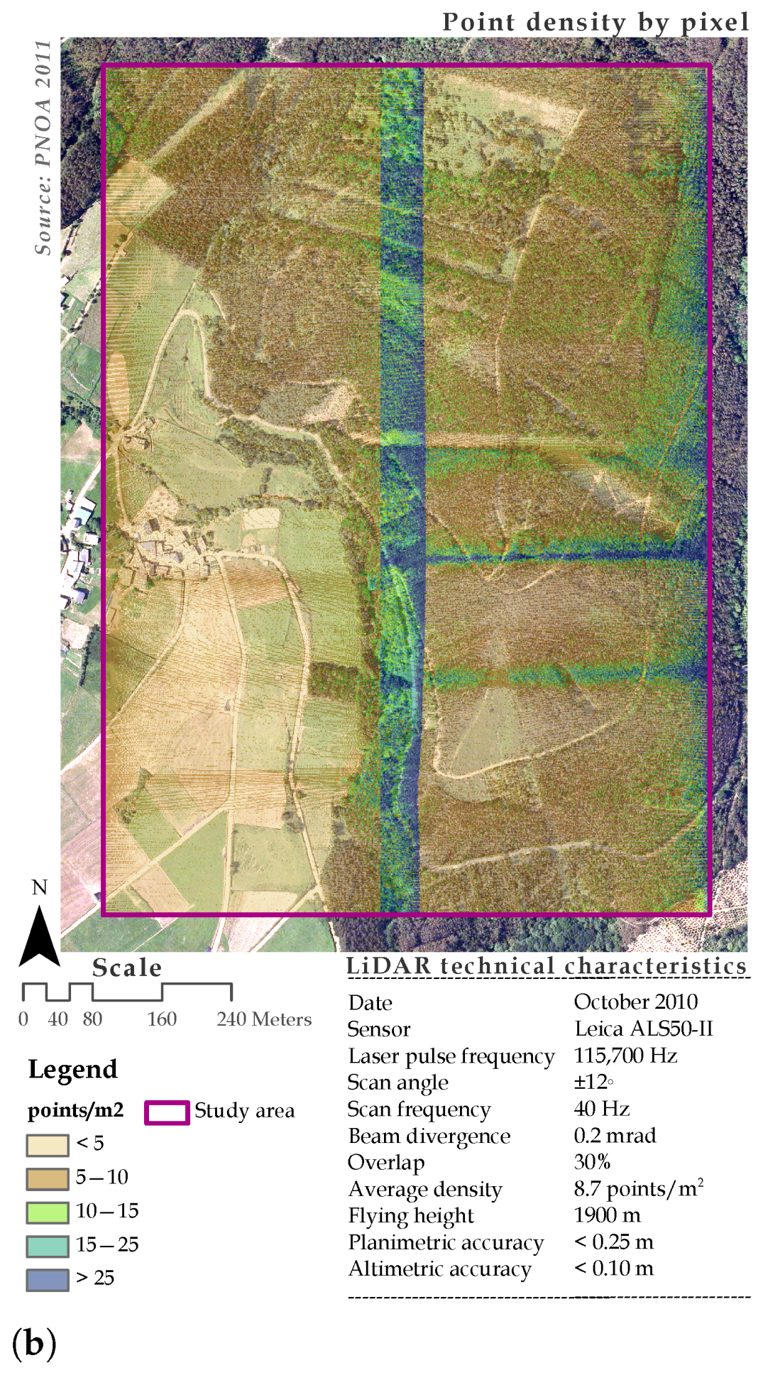
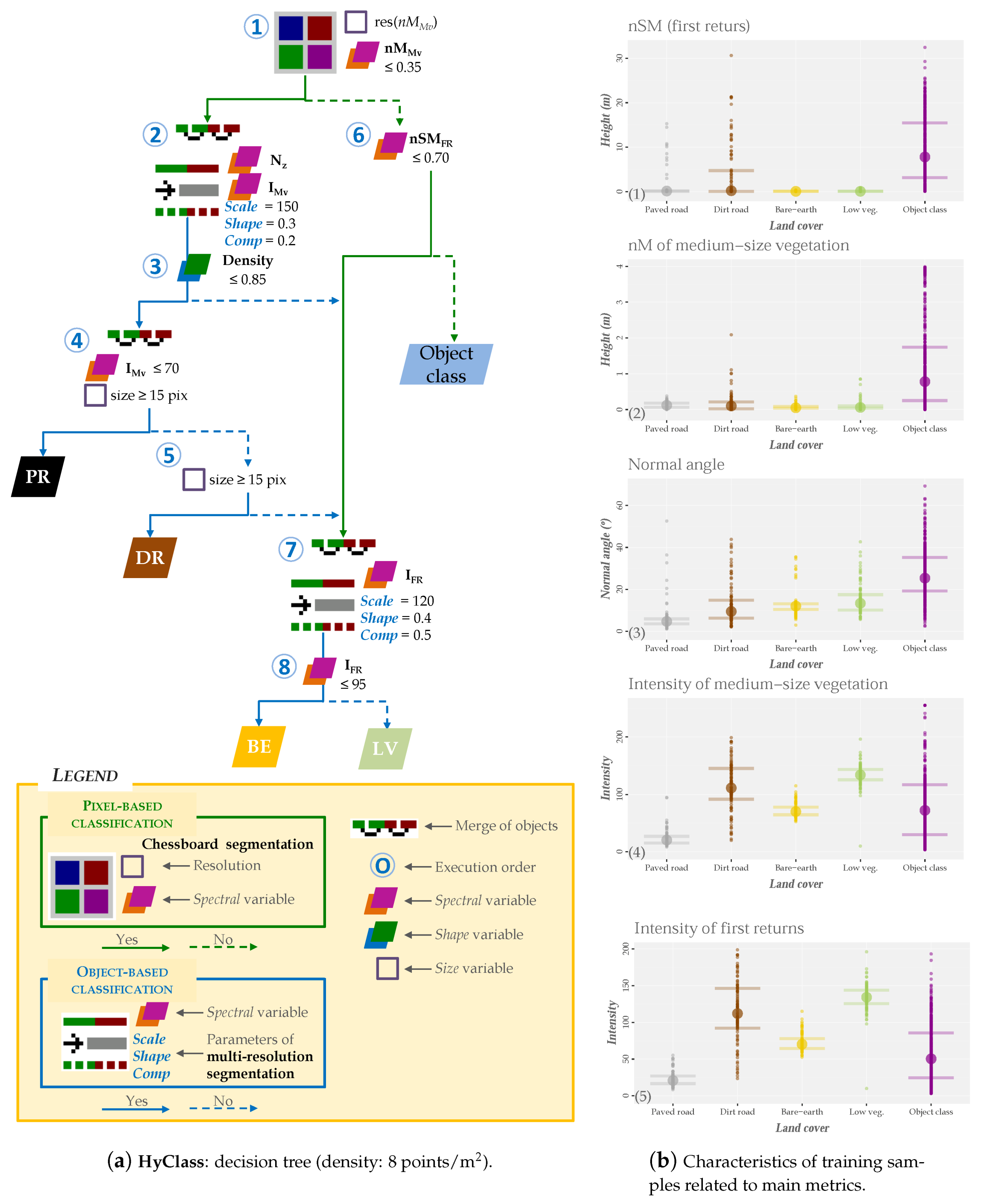
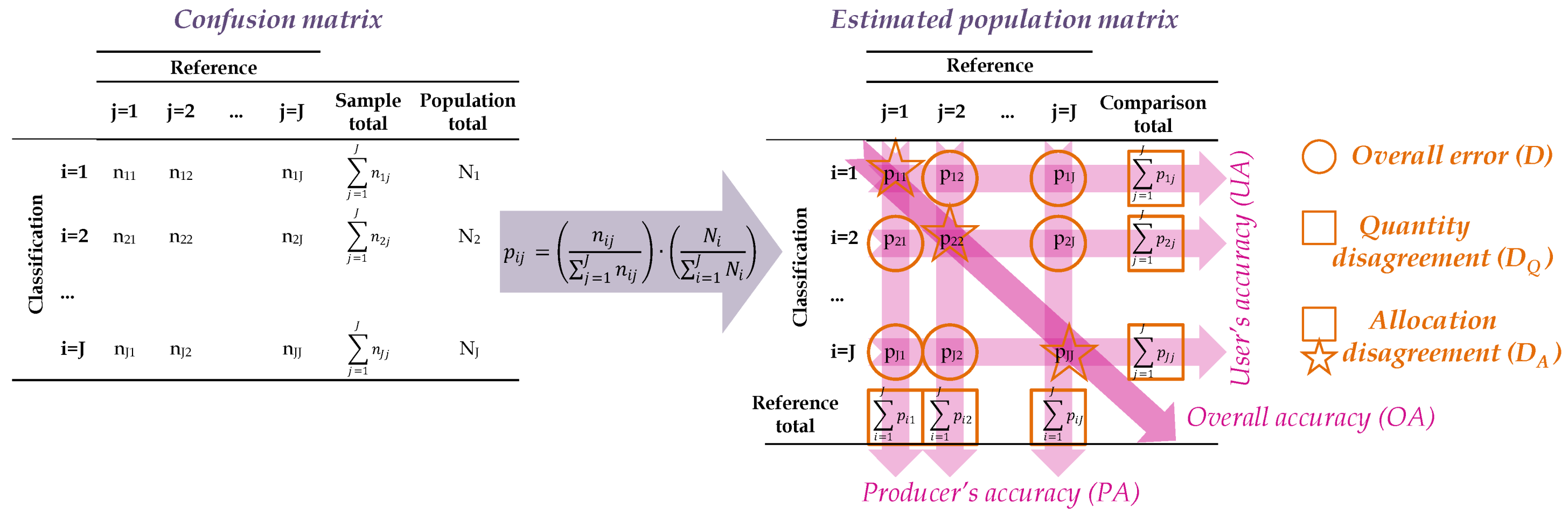
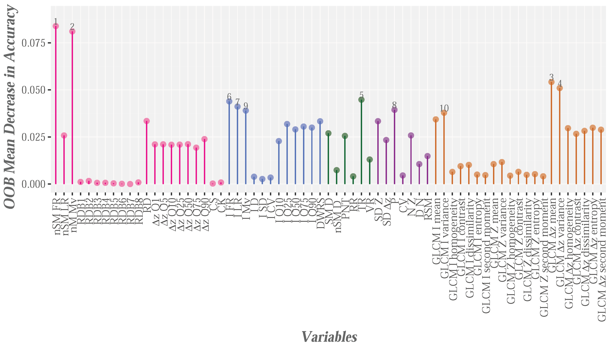
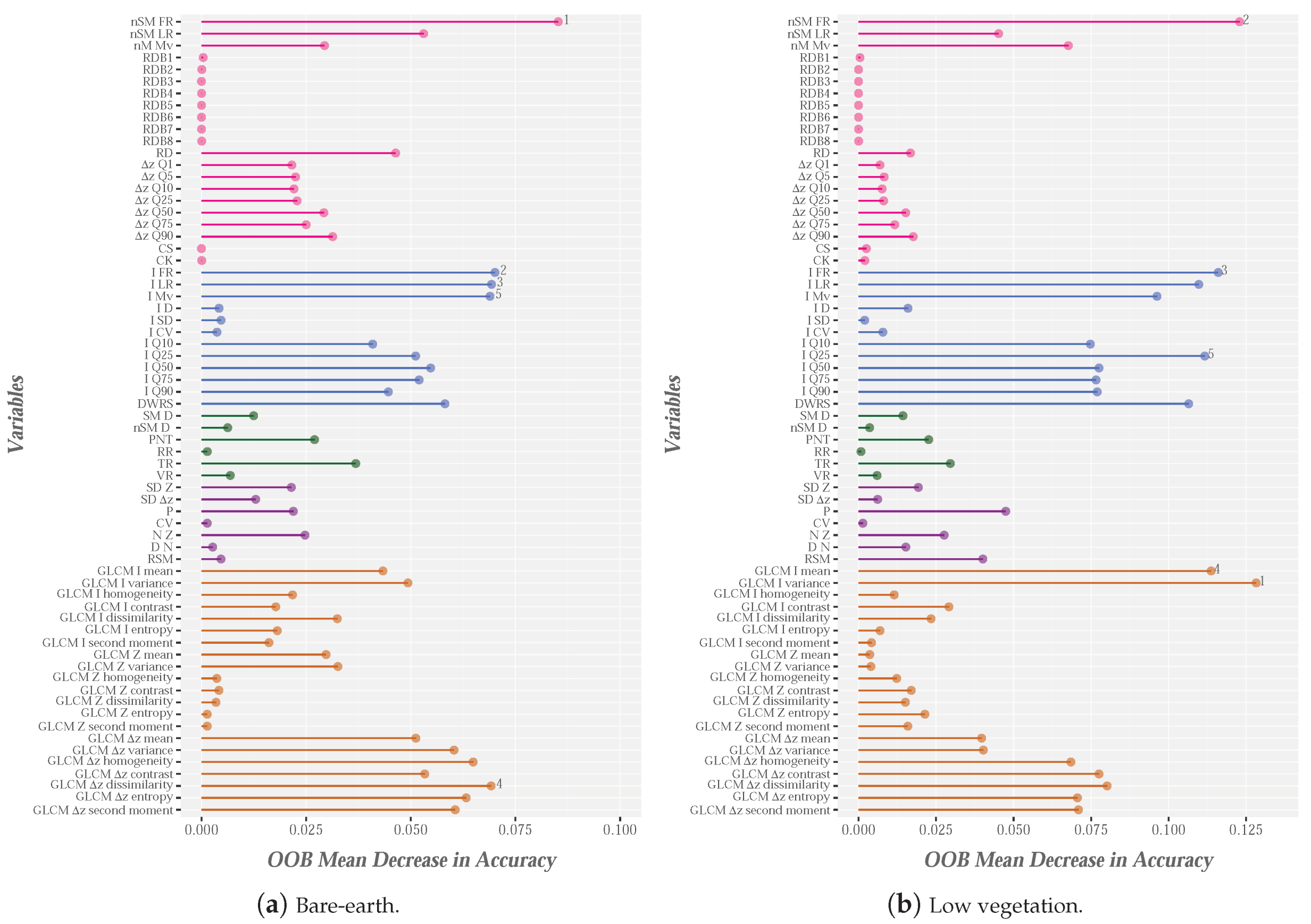
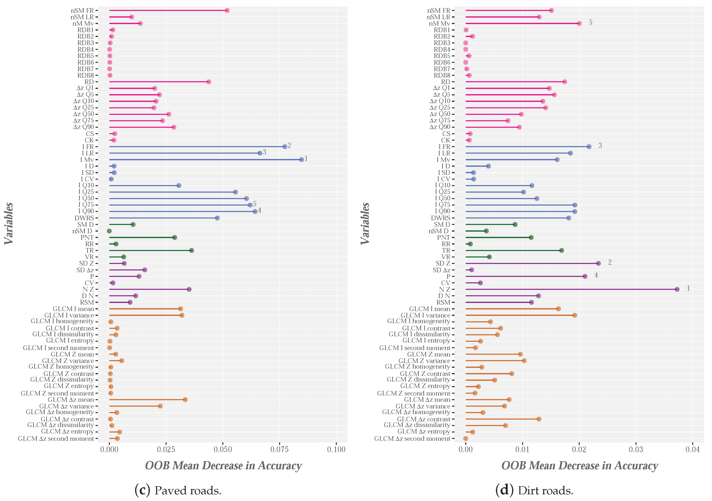
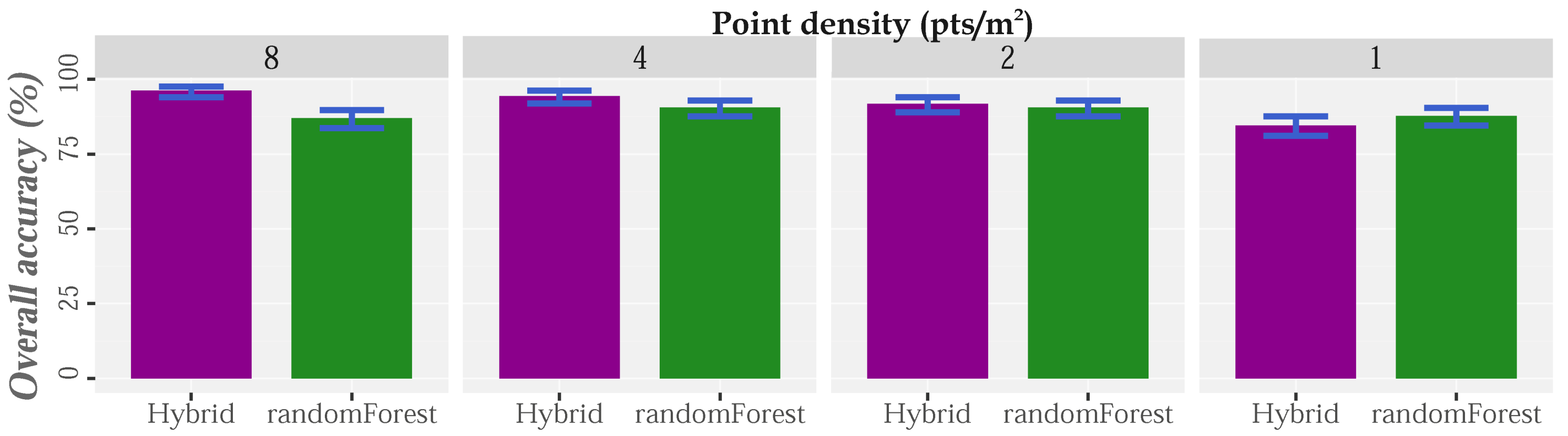
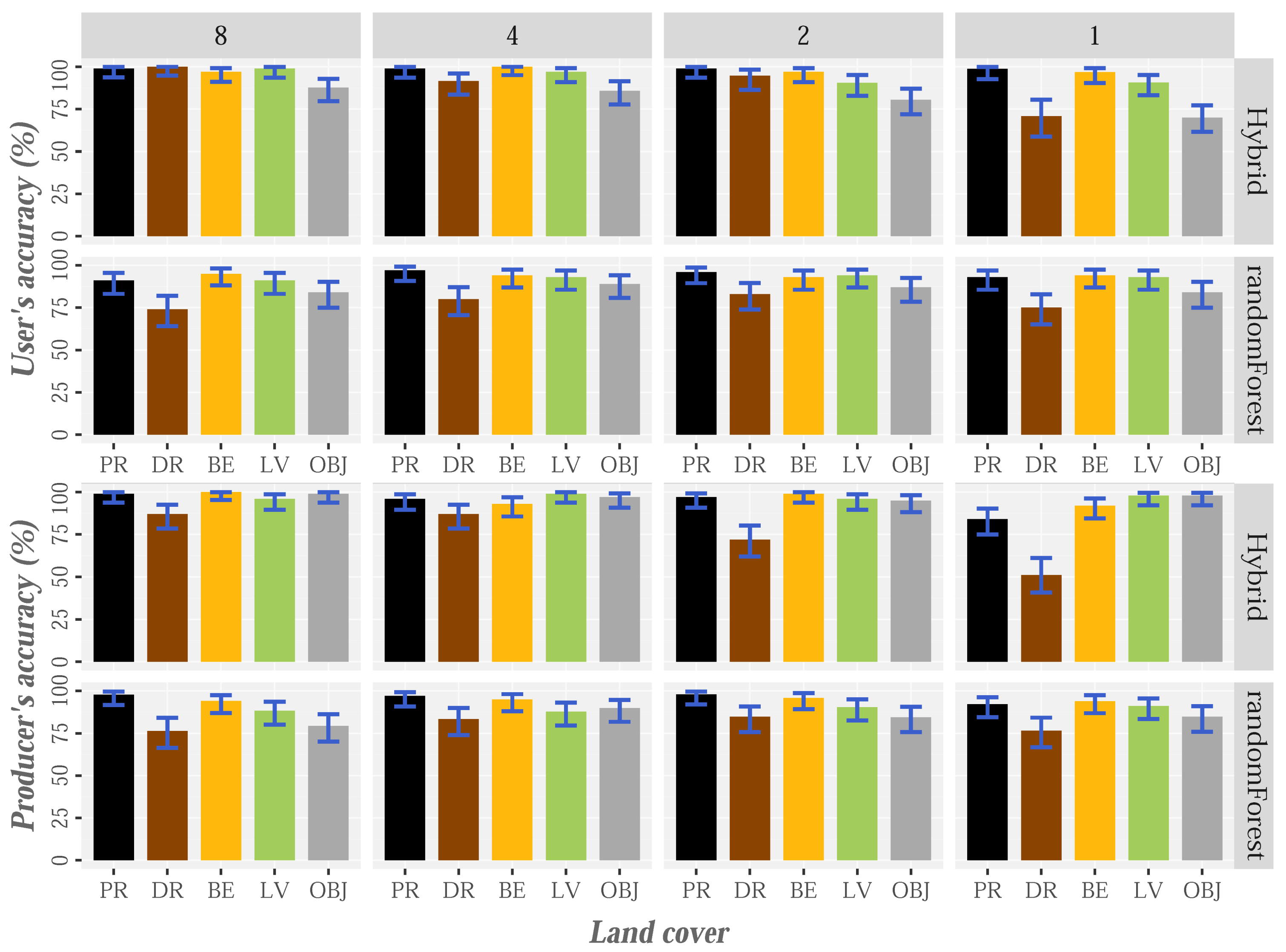
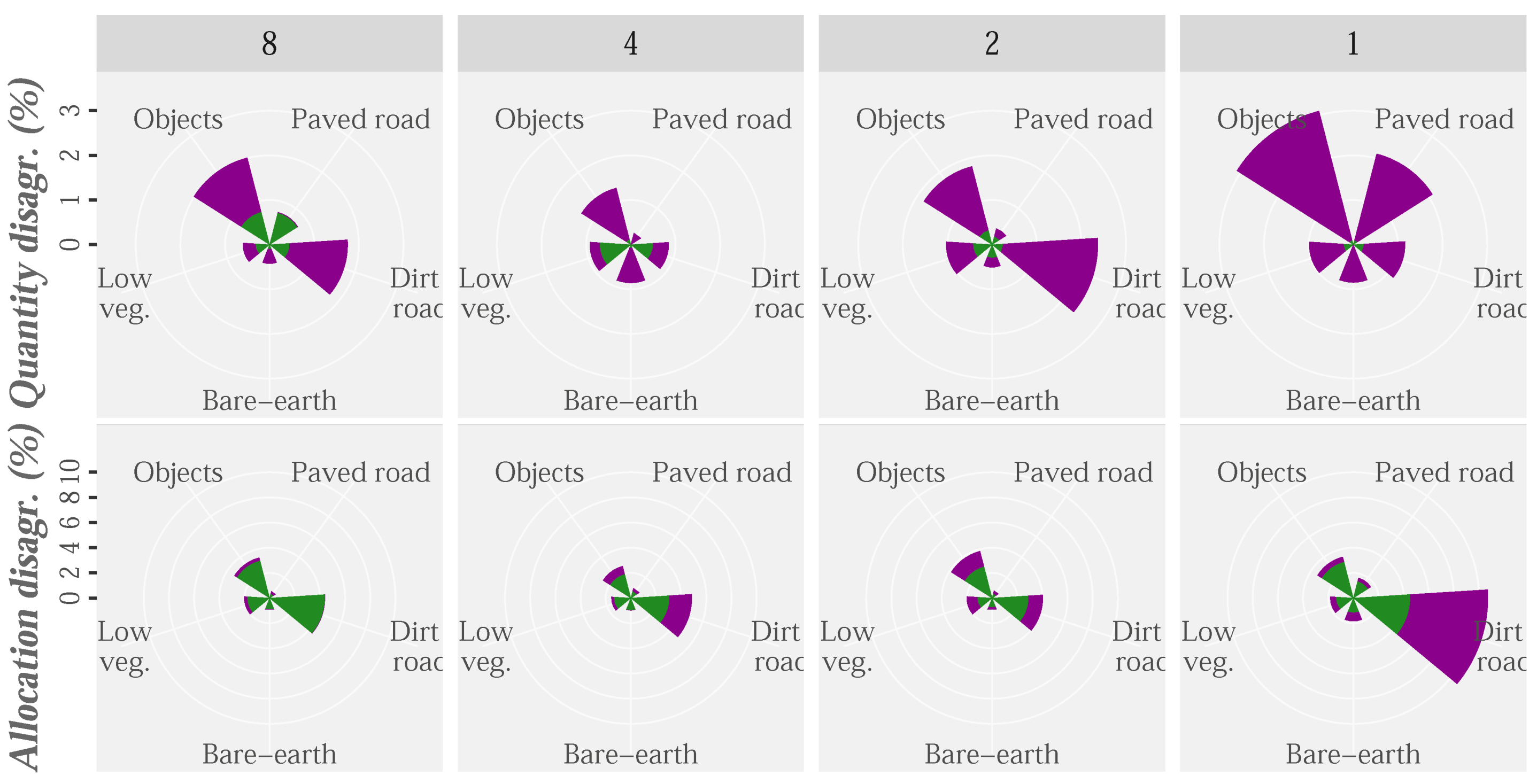
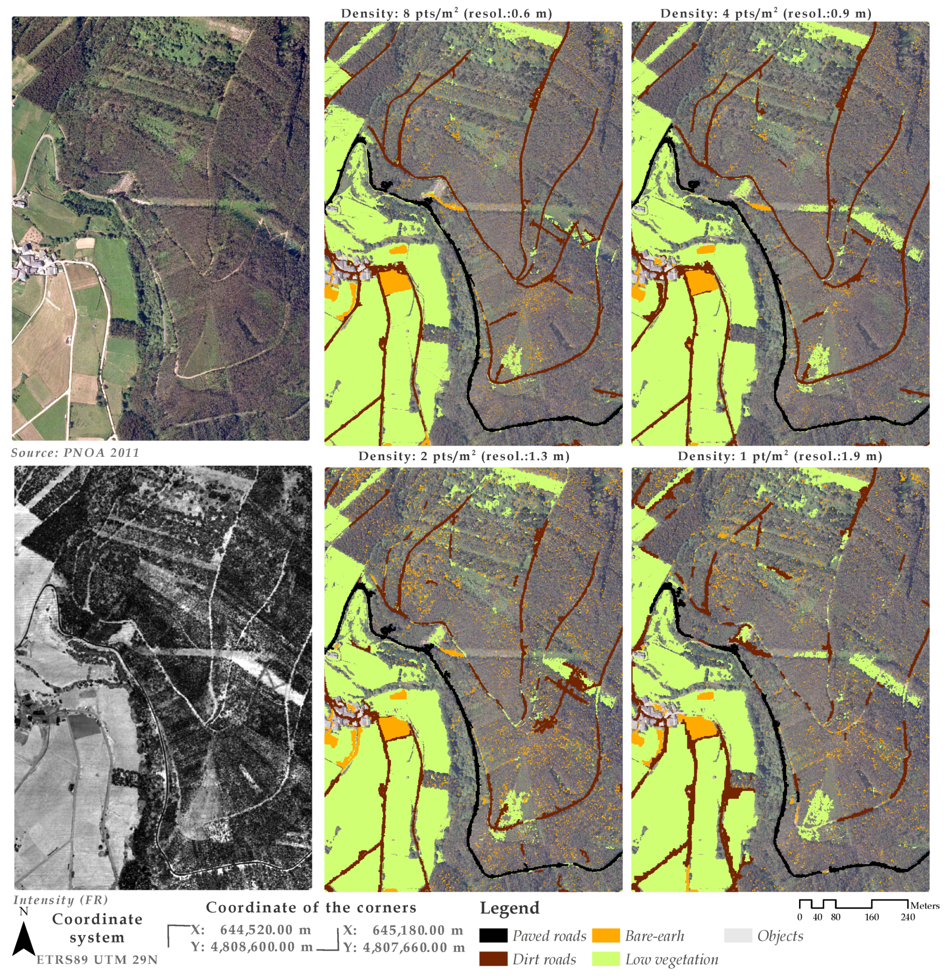
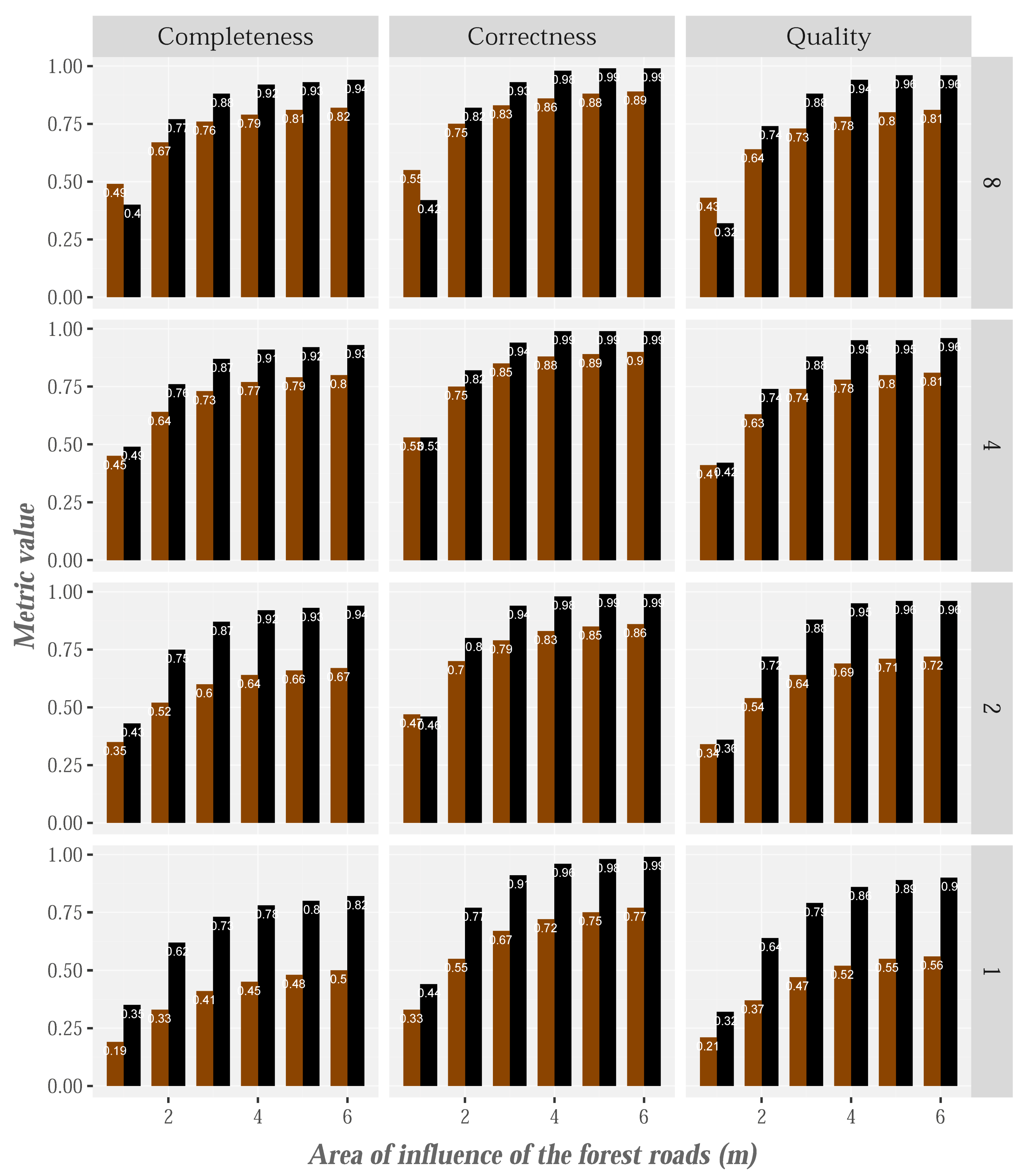
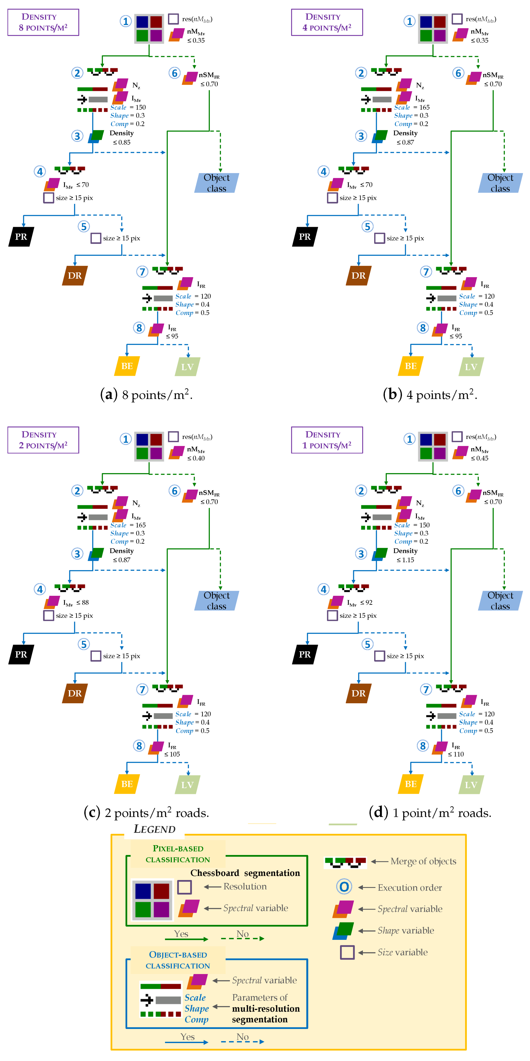
Table 1.
Summary of LiDAR metrics.
| Group | Metrics | Attributes | Description | Resol. | Ref. |
|---|---|---|---|---|---|
| E-H | nSM | Z, R | Normalized surface model from the maximum value of the first returns. | r | [48] |
| nSM | Z, R | Normalized surface model from the minimum value of the non-first returns. | r | [49] | |
| nM | Z | Normalized model of medium-sized vegetation from the maximum value of the returns which Z ≤ 4 m. | r | [50] | |
| RDB | Z | Relative density bins show the ratio between the non-groun points by height intervals and the total non-ground points in the voxel (height intervals: RDB: 0.5 m < Z ≤ 1 m; RDB: 1 m < Z ≤ 2 m; RDB: 2 m < Z ≤ 3 m; RDB: 3 m < Z ≤ 4 m; RDB: 4 m < Z ≤ 6 m; RDB: 6 m < Z ≤ 8 m; RDB: 8 m < Z ≤ 12 m; RDB: Z > 12 m). | r | [51] | |
| RD | Z | Accumulated relative density is the ratio between the non-ground points and total points in the voxel. | r | [51] | |
| Q | Z | Height percentiles show the values below which a given percentages (1%, 5%, 10%, 25%, 50%, 75%, 90%) of observations falls (minimum height threshold = 0.5 m). | r | [17] | |
| CS | Z | Coefficient of skewness measures the data asymmetry compared to a normal distribution. CS is the ratio between the third moment about the mean divided by the second moment about the mean. | r | [52] | |
| CK | Z | Coefficient of kurtosis measures the data peakedness. CK is the ratio between the fourth moment about the mean and the second moment about the mean. | r | [52] | |
| I | I | I, R | Intensity image is calculated from the 68.3% quantile of normalized intensity values of the first returns. | r | [52,53] |
| I | I, R | Intensity image is calculated from the 68.3% quantile of corrected intensity values of the non-first returns. | r | [54] | |
| I | I | Intensity image is calculated from the 68.3% quantile of corrected intensity values of the returns which Z ≤ 4 m. | r | — | |
| I | I, R | Difference of intensity between returns is the difference between the maximum intensity value of first returns and the minimum intensity value of non-first returns. If non-first returns do not exist, the minimum intensity value of first returns is considered. | r | [52] | |
| I | I | Standard deviation of the intensity. | r | [55] | |
| I | I | Coefficient of variation is the ratio of the standard deviation and mean using the LiDAR intensity data. | r | — | |
| IQ | I | Intensity percentiles show the values below which a given percentages (10%, 25%, 50%, 75%, 90%) of observations falls (minimum height threshold = 0). | r | [55] | |
| DWRS | I | Density weighted reflection sum is the sum of the corrected intensity of all returns multiplied by a correction factor. The correction factor is the mean point density of the whole dataset divided by the density at each voxel. | r | [16] | |
| Re | SM | Z, R | Difference of elevation between returns is the difference between the maximum elevation value of first returns and the minimum elevation value of non-first returns. If non-first returns do not exist, the minimum elevation value of first returns is considered. | r | [53,56] |
| nSM | Z, R | Normalized difference of height between returns is the difference between the maximum height value of first returns and the minimum height value of non-first returns divide by the sum of such values. If non-first returns do not exist, the minimum height value of first returns is considered. | r | [56,57] | |
| PNT | Z | The penetrability is the ratio between the number of points which Z ≤ 2 m and the number of total points in each voxel/cell. | r | [58,59] | |
| RR | R | Return ratio is the percentage of first and intermediate returns in each voxel/cell. | r | [49,50] | |
| TR | Z, R | Terrain return is the percentage of single and last returns in each voxel/cell. | r | [53,60] | |
| VR | Z, R | Vegetation return is the percentage of first and intermediate returns and points which Z > 12 m in each voxel/cell. | r | [53,60] | |
| Ro | SD | Z | Standard deviation of the elevation. | r | [61] |
| SD | Z | Standard deviation of the height. Only points which Z > 0.5 m are considered. | r | [50,62] | |
| P | Z | Slope image is calculated using nSM as input data. | r | [63] | |
| CV | Z | Coefficient of variation is the ratio of the standard deviation and mean using the LiDAR-derived elevation data. | r | [64] | |
| N | Z | Normal angle is calculated from the 68.3% quantile of angles (obtained for each point) between the normal vector to (see Footnote ) and the vertical axis. | r | [56,58] | |
| D | Z | Vertical distance from each point to . The maximum vertical distance of points in the voxel is the cell value. | r | [59] | |
| RSM | Z | Root mean square of D. | r | [60] | |
| T | I, I, I, I, I, I, I, I | I | Texture metrics of I, SM and nSM raster, respectively, using the grey-level co-occurrence matrix (GLCM). The calculated measures are mean, variance, contrast, dissimilarity, homogeneity, entropy, second moment and correlation, respectively. The textures are calculated using all directions. | r | [55,56] |
| Z, Z, Z, Z, Z, Z, Z, Z | SM | r | [50,65] | ||
| Z, Z, Z, Z, Z, Z, Z, Z | nSM | r | [61,62] |
Groups of metrics: E-H, elevation/height; I, intensity; Re, returns; Ro, roughness; T, texture. Attributes: Z is the elevation; I is the normalized intensity value; R is the return number; and Z is the normalized height. To calculate the angle between the normal vector to and the vertical axis for each point, it is necessary first to obtain the plane for each point. From each point in the voxel, the neighboring points, whose elevation difference in relation to this point is , are selected. These points are then used to fit a plane () by means of a linear model and using the glm function (stats package in R software v.4.0.2) [42].
Table 2.
Main quality measures.
| Equation | Description | Ref. |
|---|---|---|
| The ratio of the records correctly extracted to the total number of relevant records within the ground-truth data, i.e., the percentage of the reference roads which could be extracted. Optimum value = 1. | [3,12,20,81,82,83,84,85] | |
| The ratio of the number of relevant records extracted to the total number of relevant and irrelevant records retrieved, i.e., the percentage of correctly extracted road data. Optimum value = 1. | [3,12,20,81,82,83,84] | |
| The ratio of the overlapping area of extracted records and ground-truth records to the total area. It is a measure of the goodness of the final result combining completeness and correctness into a single measure. Optimum value = 1. | [3,12,20,81,82,83,84,85] | |
| This measure is a powerful evaluation ratio for the harmonic mean of completeness and correctness. | [83,84,85] | |
| The number of gaps per kilometer represents the number of gaps in the reference data. It is an indicator for the fragmentation of the extraction results. Optimal value = 0. | [81] | |
| This measure shows the average number of gap length per gap in the study area. This measure helps in analyzing the fragmentation of the extracted output. Optimal value = 0. | [81,84] |
Following the notation used in previous research [20,81], TP (true positive) refers to the number of road segments that have been correctly identified as road; FP (false positive) refers to the number of road segments that have been incorrectly identified as road; TN (true negative) refers to the number of non-road objects that have been correctly identified as non-road; and FN (false negative) refers to the number of reference road segments that have not been identified as road. l, number of pieces of matched extraction; d(extr; ref), shortest distance between the ith piece of the matched extraction and the reference network; n, number of gaps; L, length of reference (km); gl, length of the ith gap (m).
Table 3.
Completeness in relation to the roads occluded by canopy cover (area of influence = 3 m, value proposed by Doucette et al. [94]).
Table 3.
Completeness in relation to the roads occluded by canopy cover (area of influence = 3 m, value proposed by Doucette et al. [94]).
| Roads Totally or Partially Included Below Canopy Cover | 8 point/m | 4 point/m | 2 point/m | 1 point/m | ||||
|---|---|---|---|---|---|---|---|---|
| PR | DR | PR | DR | PR | DR | PR | DR | |
| Yes | 91% | 78% | 91% | 75% | 91% | 61% | 79% | 37% |
| No | 95% | 85% | 93% | 84% | 94% | 71% | 79% | 59% |
Table 4.
Analysis of variance (ANOVA) for the effects of penetrability, slope, road surface and point density on the quality measures and figure shows the results of plot.design function.
Table 4.
Analysis of variance (ANOVA) for the effects of penetrability, slope, road surface and point density on the quality measures and figure shows the results of plot.design function.
| Factors | |||||
|---|---|---|---|---|---|
| Penetrability | Slope | Road Surface | Ponit Density | ||
| Completeness | Df | 4 | 2 | 1 | 3 |
| F value | 5.394 | 85.222 | 7.632 | 5.068 | |
| Pr (>F) | *** | *** | ** | ** | |
| Correctness | Df | 4 | 2 | 1 | 3 |
| F value | 0.890 | 24.296 | 17.776 | 4.656 | |
| Pr (>F) | 0.4734 | *** | *** | ** | |
| Quality | Df | 4 | 2 | 1 | 3 |
| F value | 4.279 | 62.663 | 27.715 | 4.328 | |
| Pr (>F) | ** | *** | *** | ** | |
 | |||||
Statistical significance: *** 0.001; ** 0.01.
Publisher’s Note: MDPI stays neutral with regard to jurisdictional claims in published maps and institutional affiliations. |
© 2021 by the authors. Licensee MDPI, Basel, Switzerland. This article is an open access article distributed under the terms and conditions of the Creative Commons Attribution (CC BY) license (http://creativecommons.org/licenses/by/4.0/).
Share and Cite
MDPI and ACS Style
Buján, S.; Guerra-Hernández, J.; González-Ferreiro, E.; Miranda, D. Forest Road Detection Using LiDAR Data and Hybrid Classification. Remote Sens. 2021, 13, 393. https://0-doi-org.brum.beds.ac.uk/10.3390/rs13030393
AMA Style
Buján S, Guerra-Hernández J, González-Ferreiro E, Miranda D. Forest Road Detection Using LiDAR Data and Hybrid Classification. Remote Sensing. 2021; 13(3):393. https://0-doi-org.brum.beds.ac.uk/10.3390/rs13030393
Chicago/Turabian StyleBuján, Sandra, Juan Guerra-Hernández, Eduardo González-Ferreiro, and David Miranda. 2021. "Forest Road Detection Using LiDAR Data and Hybrid Classification" Remote Sensing 13, no. 3: 393. https://0-doi-org.brum.beds.ac.uk/10.3390/rs13030393
Note that from the first issue of 2016, this journal uses article numbers instead of page numbers. See further details here.