
A Semi-Physical Approach for Downscaling Satellite Soil Moisture Data in a Typical Cold Alpine Area, Northwest China


Abstract
:
1. Introduction
2. Study Area and Data
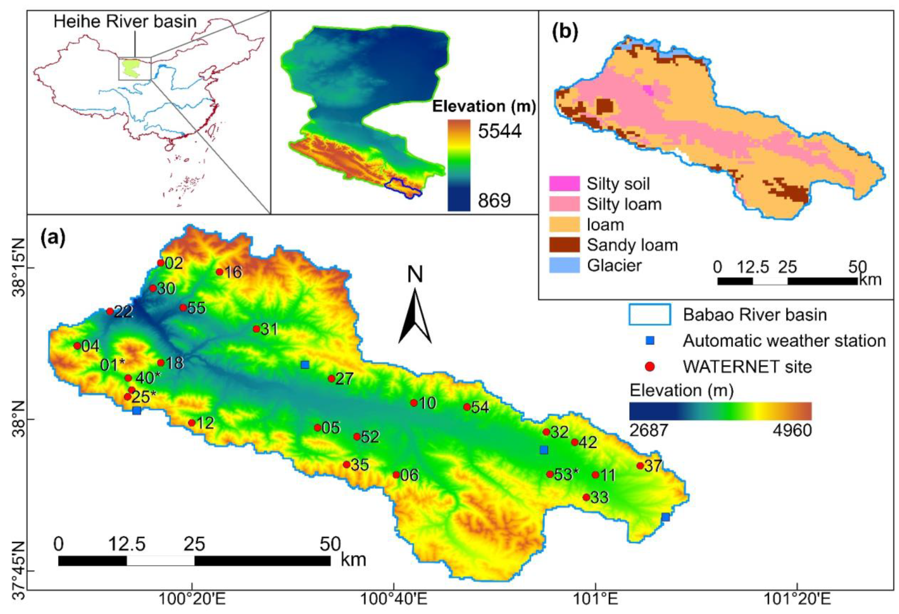
2.1. Study Area
2.2. SMAP Data
2.3. MODIS Land Surface Temperature and Reflectance
2.4. Soil Texture Data
2.5. In-Situ Data
3. Methodology
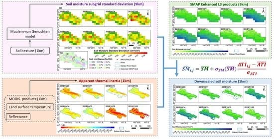
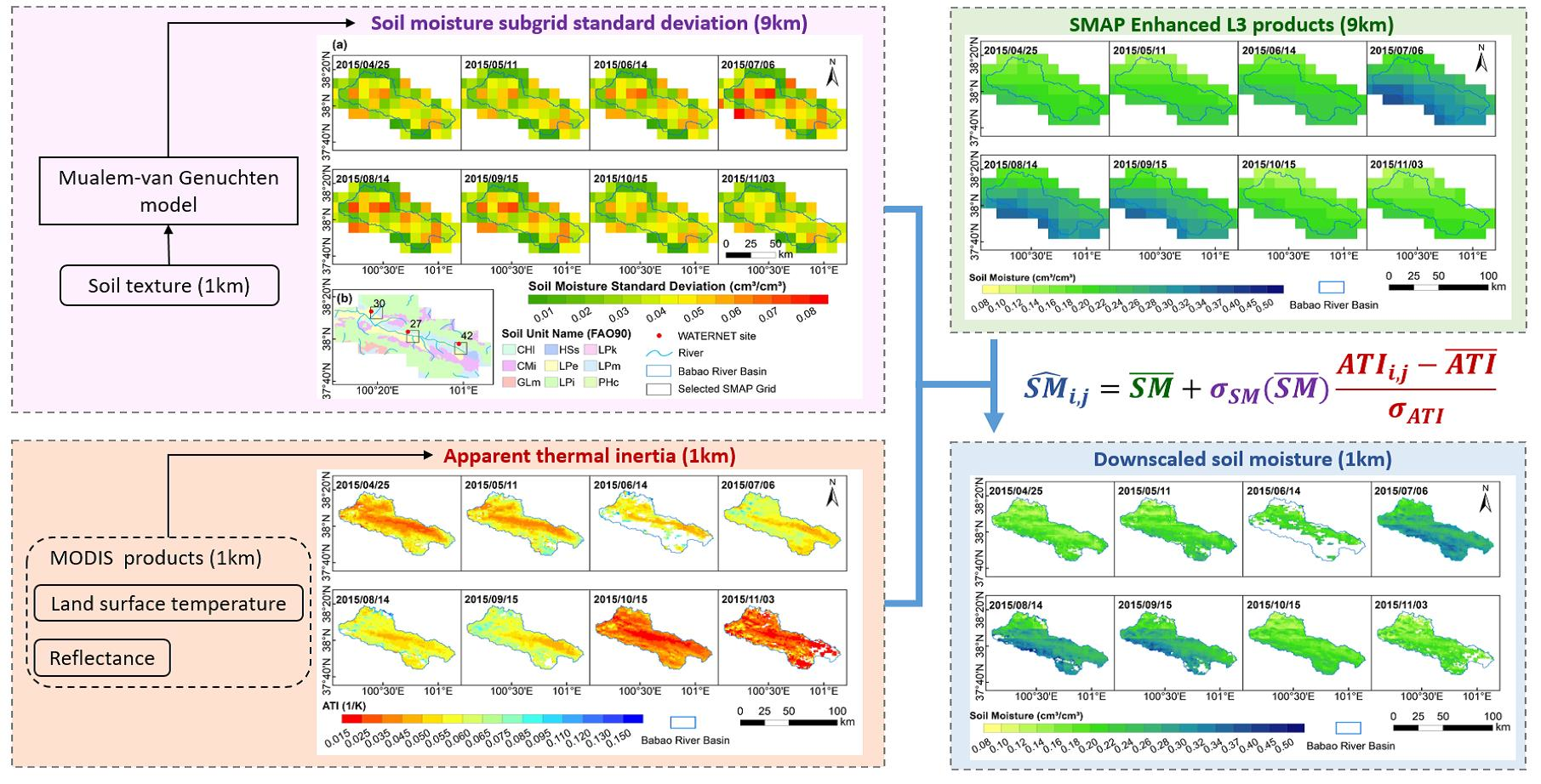
3.1. Formulation
3.2. Calculation of Subgrid SM Standard Deviations
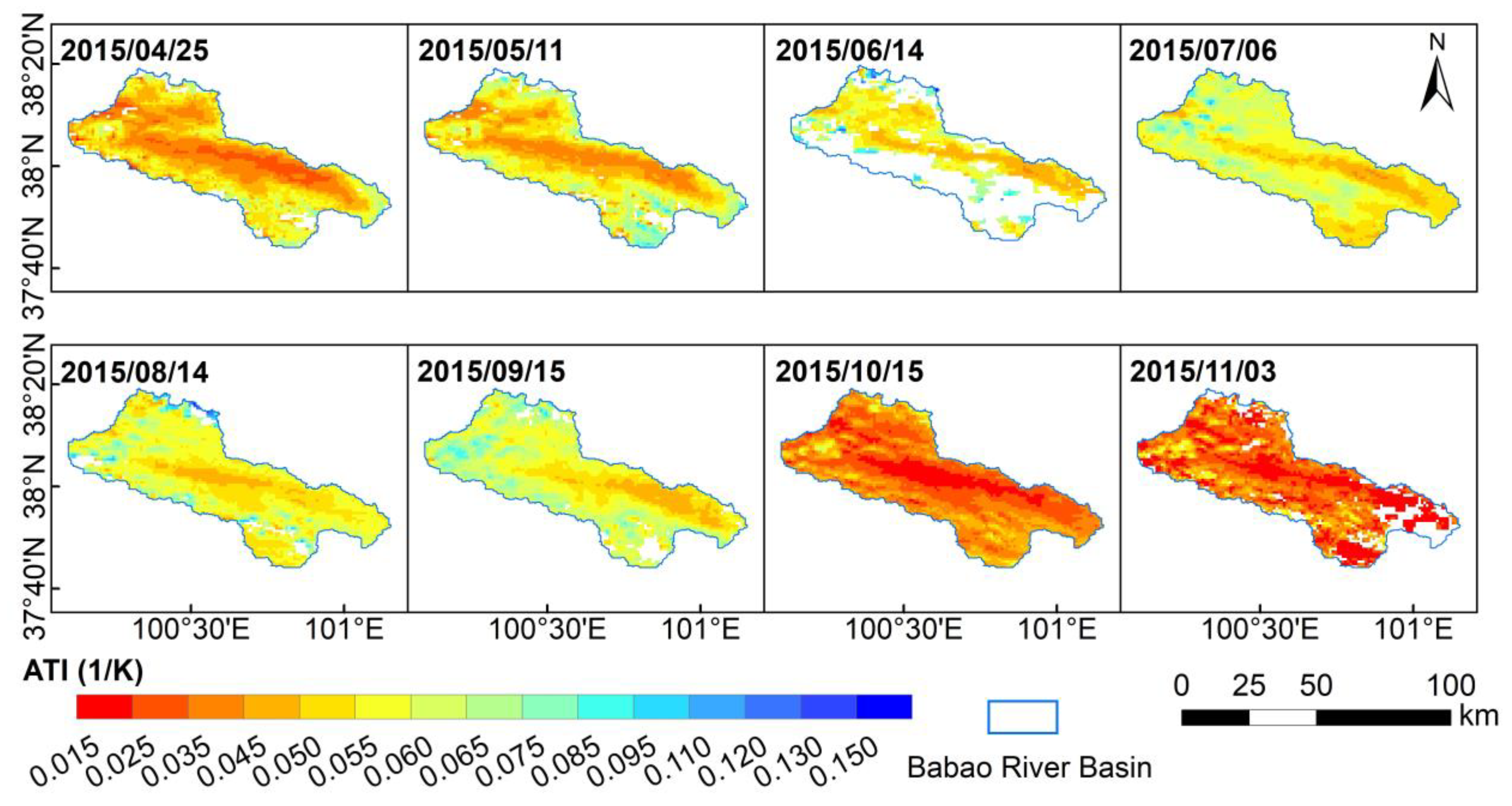
3.3. Calculation of Apparent Thermal Inertia
3.4. Evaluation and Validation
4. Results
4.1. Assessment of the SMAP Data
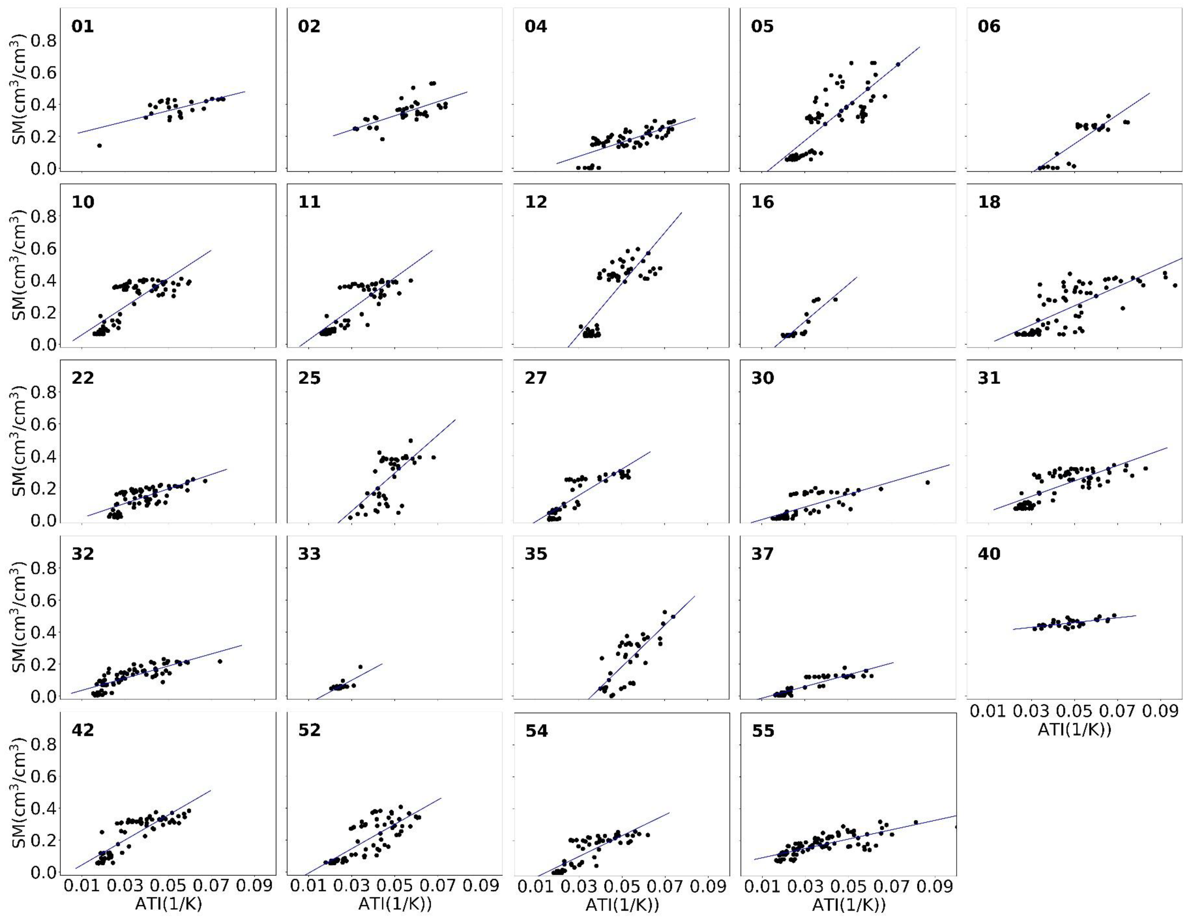
4.2. Linearity between ATI and Soil Moisture
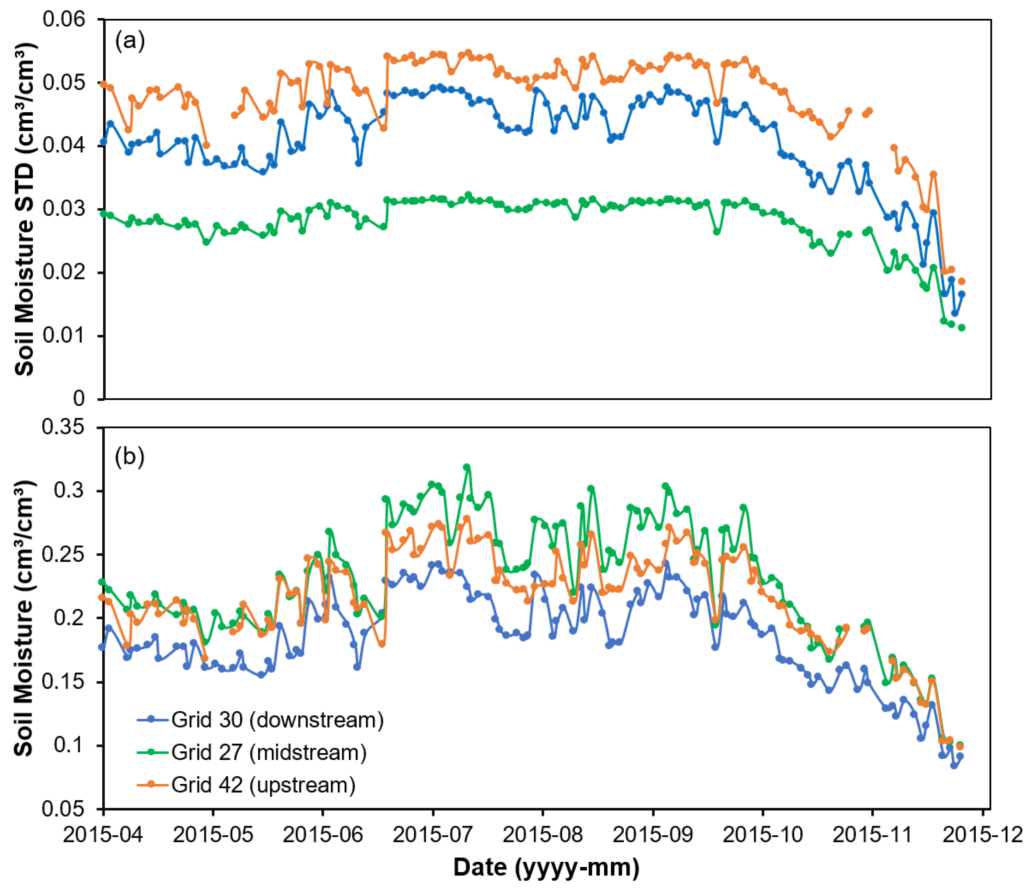
4.3. Estimated Subgrid Standard Deviations for the SMAP Grid
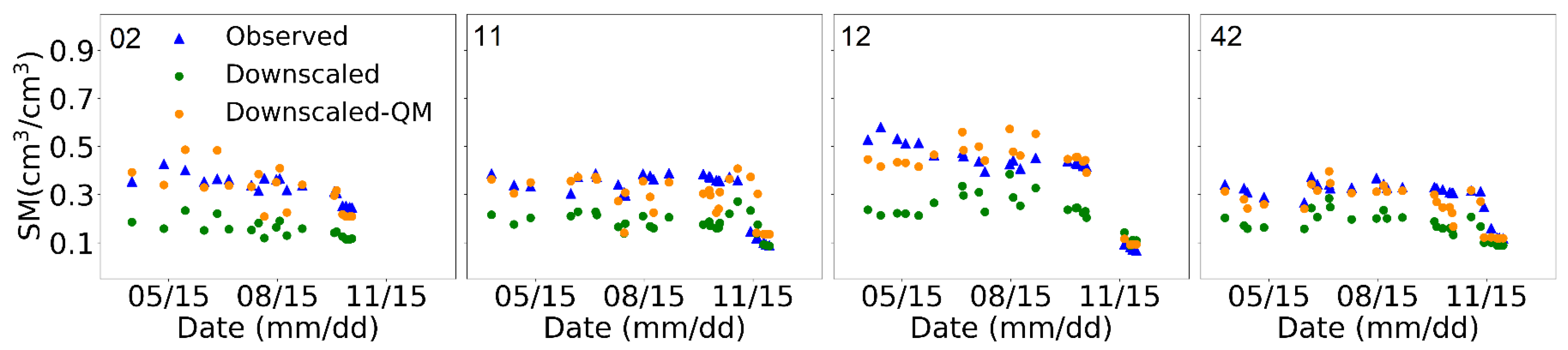
4.4. Validation of Downscaled Results
5. Discussions
6. Conclusions
- (1)
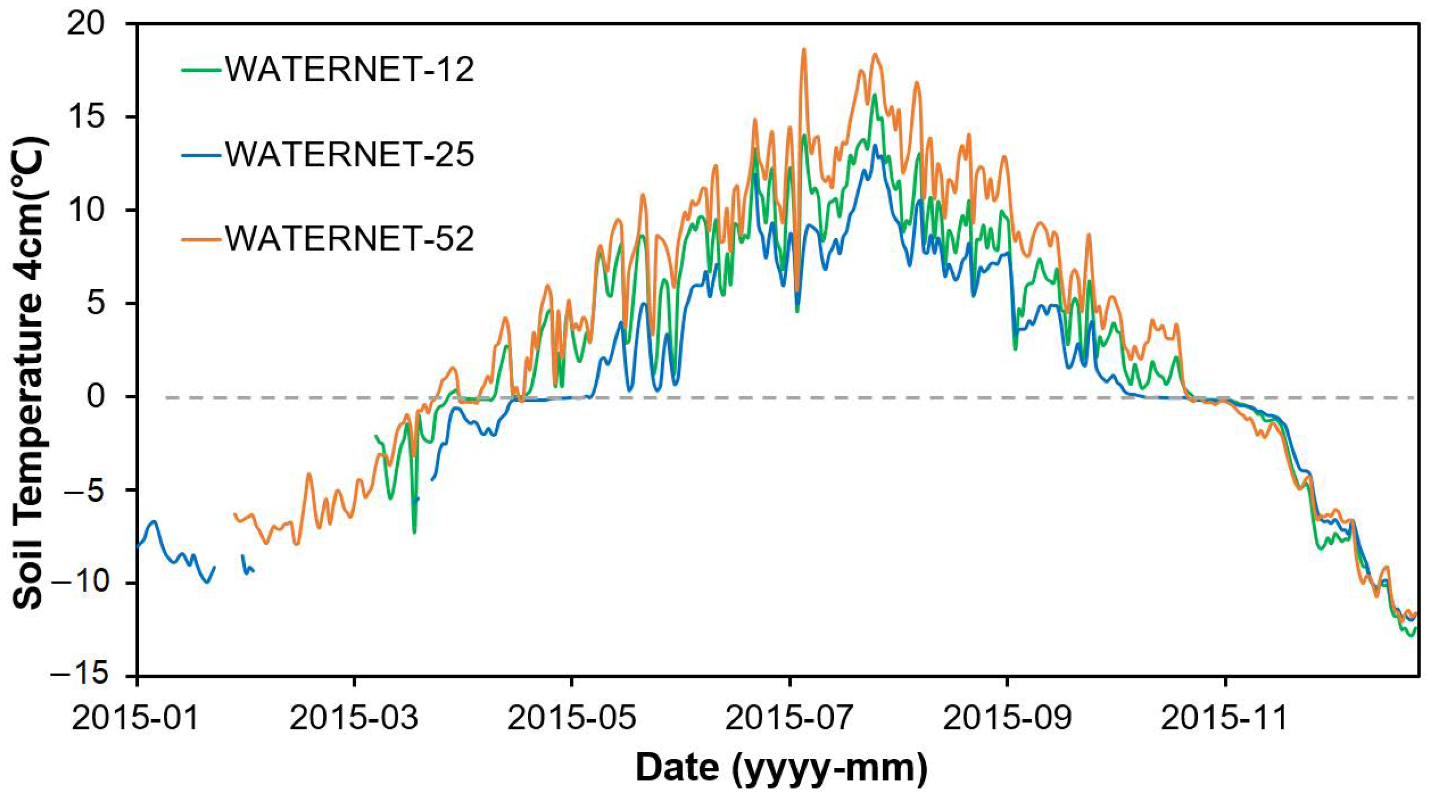
- In cold alpine areas, in situ SM observations present site-wise good linearity with the calculated ATI values, satisfying the mathematical assumption of linearity behind our approach. Similar seasonality and spatial distribution were found in SM and ATI. The mean between ATI and the in-situ SM observations were measured as 0.61 at all WATERNET sites in the BRB.
- (2)
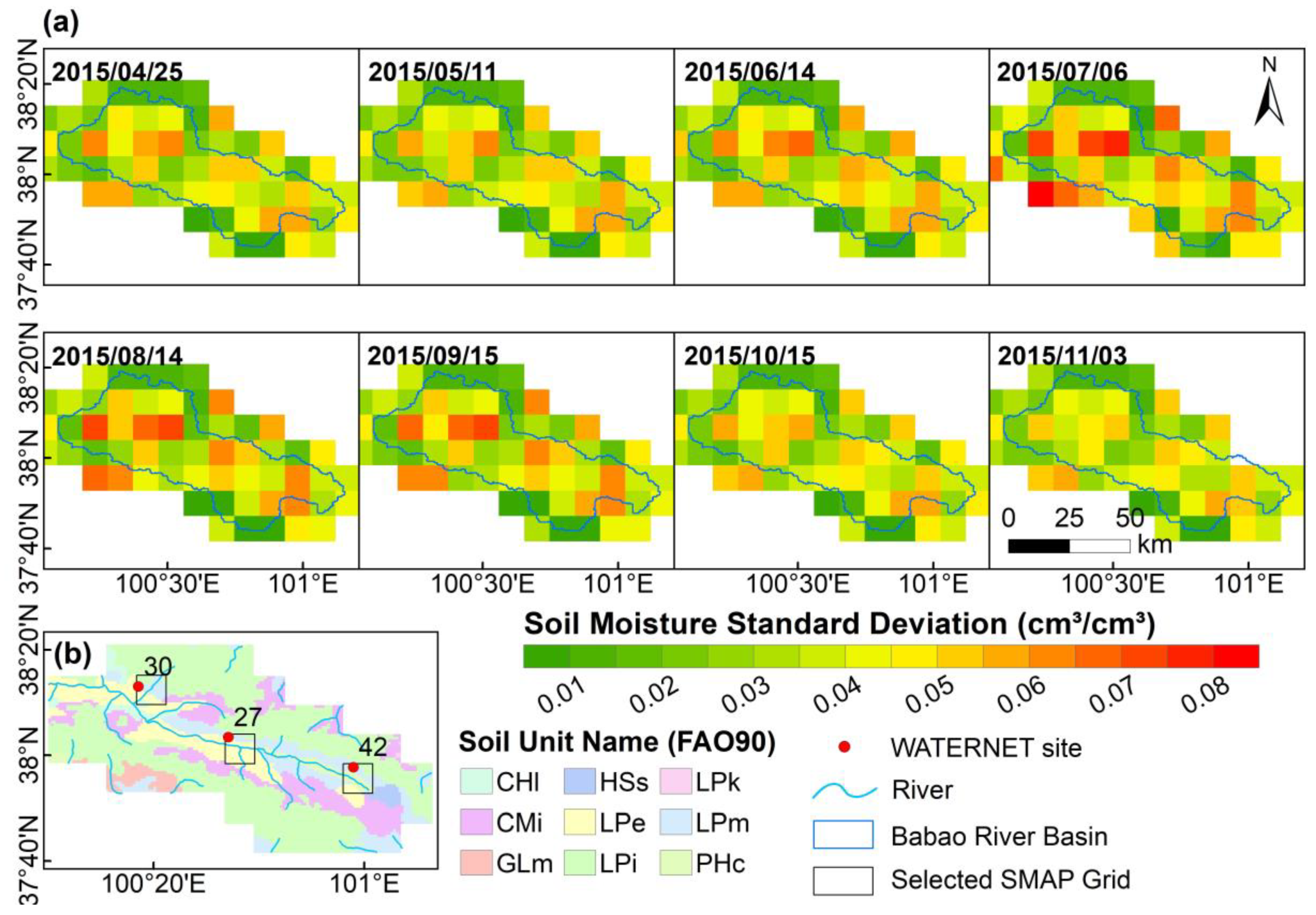
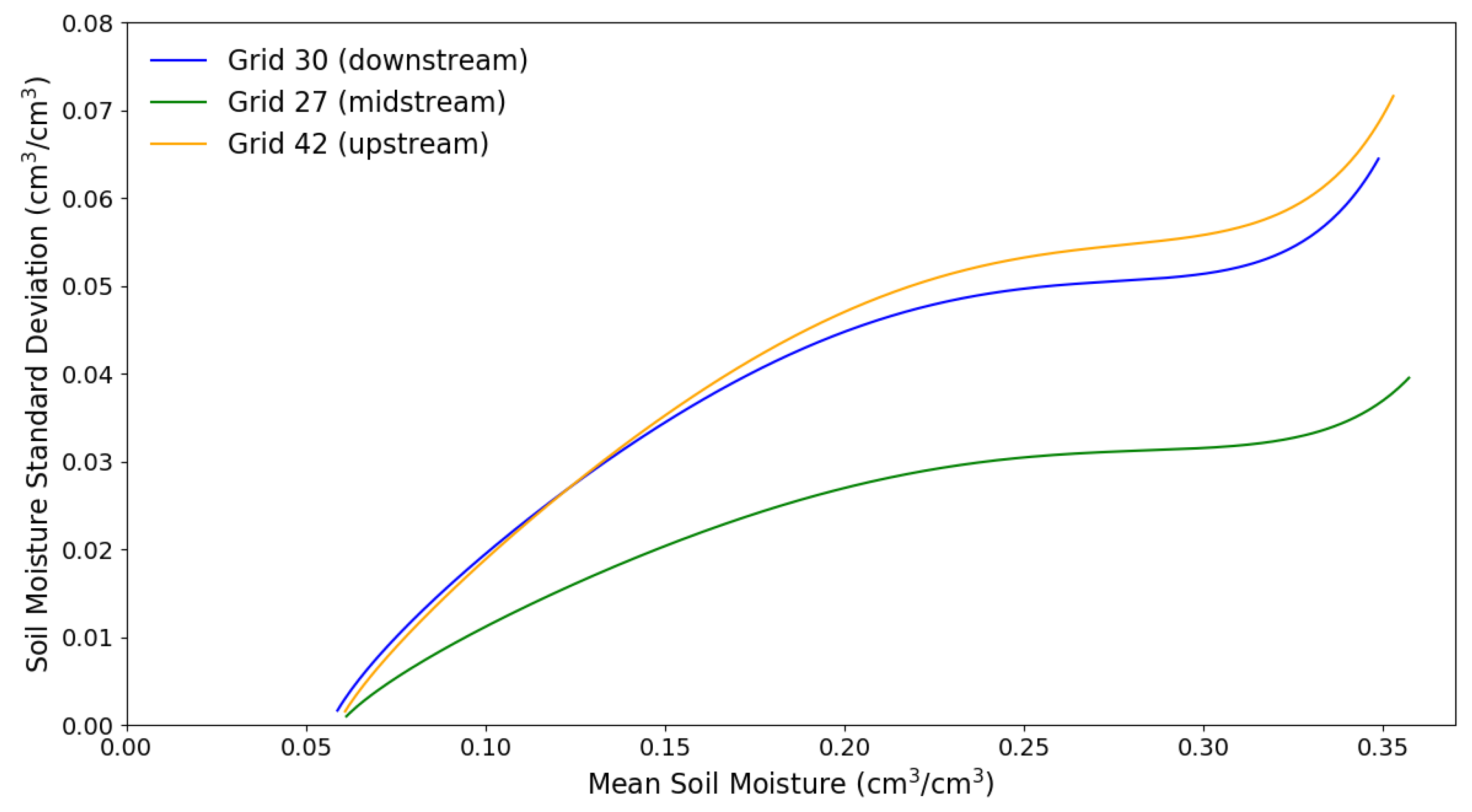
- Sub grid SM standard deviation is used to account for SM heterogeneity in the approach and they were successfully estimated by the MvG model fed with fine-resolution soil texture data.
- (3)
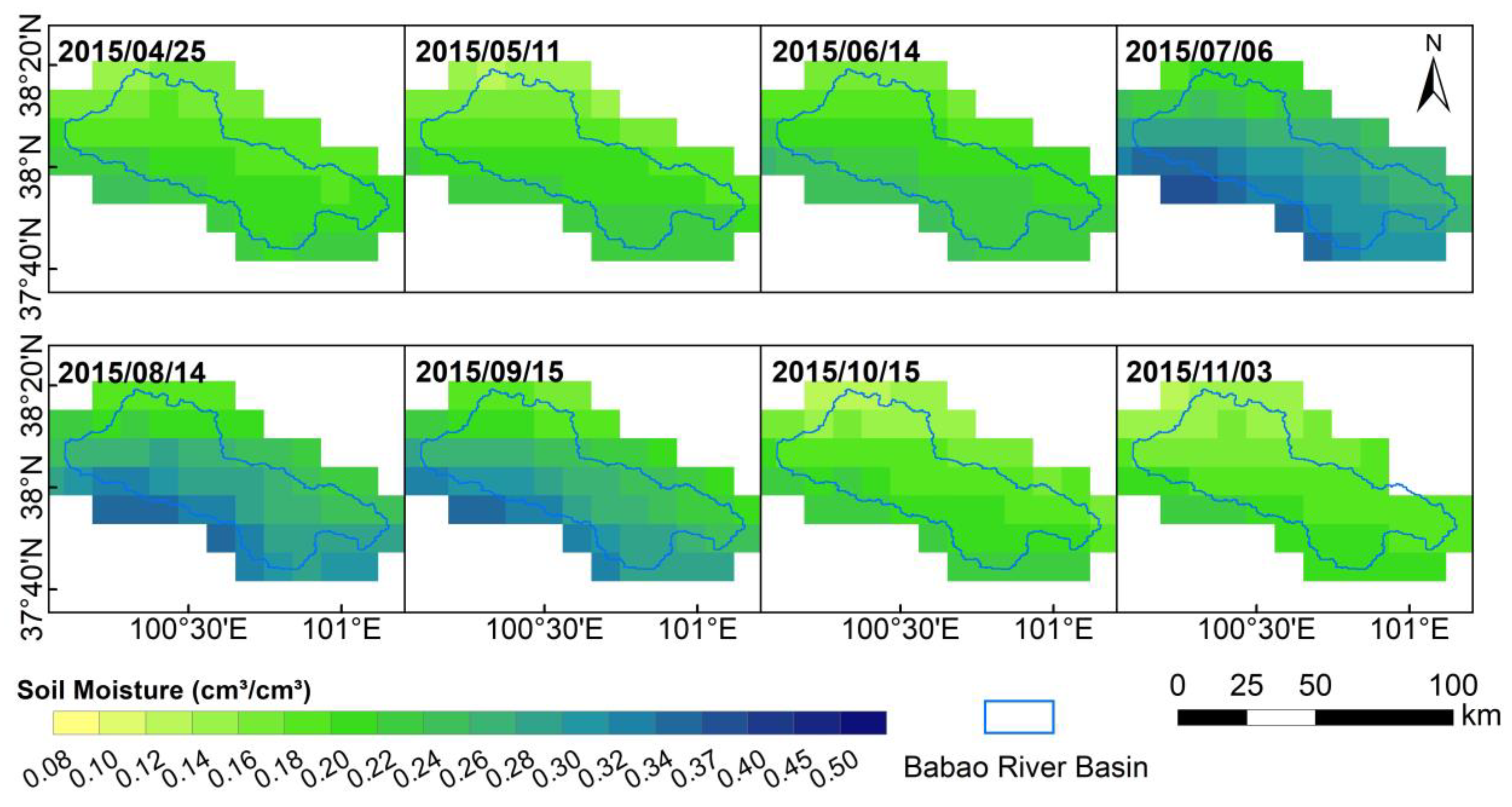
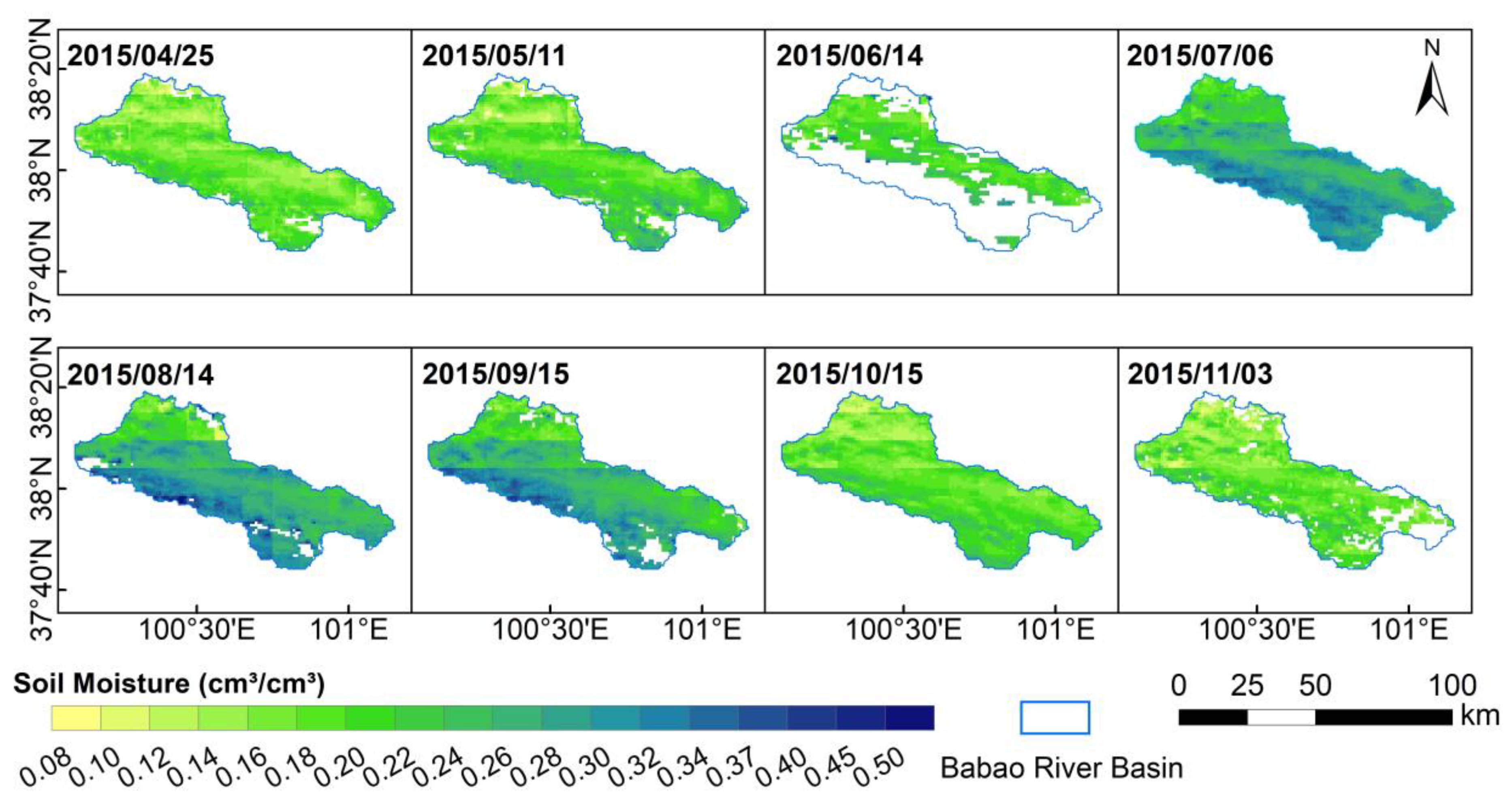
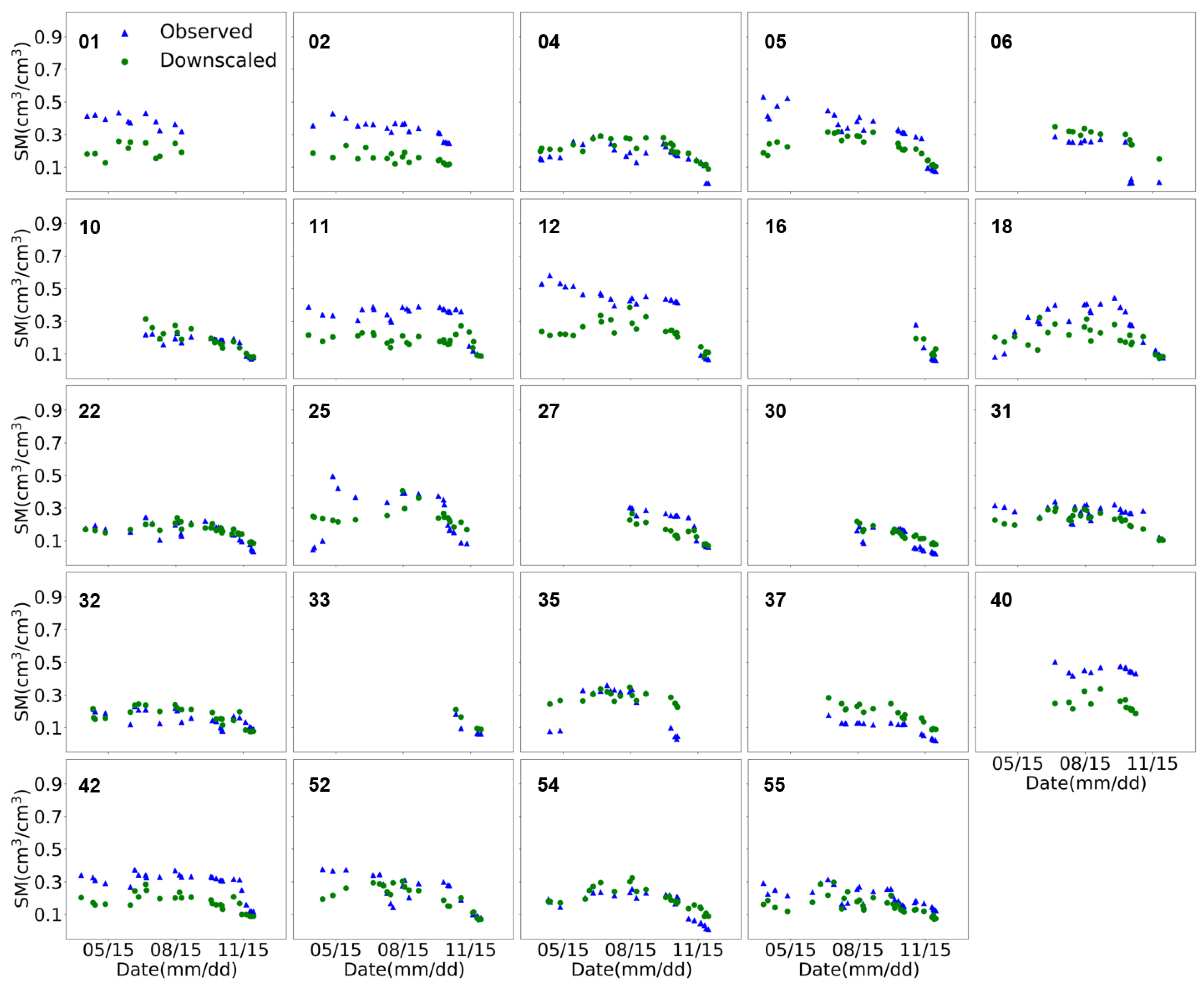
- The downscaled 1-km resolution SM data showed reasonable spatial and temporal patterns in the BRB and well agreed with in situ SM observations, with an average correlation coefficient of 0.742 and small RMSE, MAE and ubRMSE values. After removing systematic errors contained in the original SMAP data from the downscaled results reassessing the performance showed better metric values, further confirming the effectiveness of the downscaling approach.
Author Contributions
Funding
Institutional Review Board Statement
Informed Consent Statement
Data Availability Statement
Acknowledgments
Conflicts of Interest
References
- Sabaghy, S.; Walker, J.P.; Renzullo, L.J.; Jackson, T.J. Spatially enhanced passive microwave derived soil moisture: Capabilities and opportunities. Remote Sens. Environ. 2018, 209, 551–580. [Google Scholar] [CrossRef]
- Peng, J.; Loew, A.; Merlin, O.; Verhoest, N.E. A review of spatial downscaling of satellite remotely sensed soil moisture. Rev. Geophys. 2017, 55, 341–366. [Google Scholar] [CrossRef]
- Entekhabi, D.; Njoku, E.G.; Neill, P.E.O.; Kellogg, K.H.; Crow, W.T.; Edelstein, W.N.; Entin, J.K.; Goodman, S.D.; Jackson, T.J.; Johnson, J.; et al. The soil moisture active passive (SMAP) mission. Proc. IEEE 2010, 98, 704–716. [Google Scholar] [CrossRef]
- Seneviratne, S.I.; Corti, T.; Davin, E.L.; Hirschi, M.; Jaeger, E.B.; Lehner, I.; Orlowsky, B.; Teuling, A.J. Investigating soil moisture-climate interactions in a changing climate: A review. Earth Sci. Rev. 2010, 99, 125–161. [Google Scholar] [CrossRef]
- Collow, T.W.; Robock, A.; Basara, J.B.; Illston, B.G. Evaluation of SMOS retrievals of soil moisture over the central United States with currently available in situ observations. J. Geophys. Res. Atmosph. 2012, 117. [Google Scholar] [CrossRef] [Green Version]
- Crow, W.T.; Berg, A.A.; Cosh, M.H.; Loew, A.; Mohanty, B.P.; Panciera, R.; de Rosnay, P.; Ryu, D.; Walker, J.P. Upscaling sparse ground-based soil moisture observations for the validation of coarse-resolution satellite soil moisture products. Rev. Geophys. 2012, 50. [Google Scholar] [CrossRef] [Green Version]
- Bogena, H.R.; Herbst, M.; Huisman, J.A.; Rosenbaum, U.; Weuthen, A.; Vereecken, H. Potential of wireless sensor networks for measuring soil water content variability. Vadose Zone J. 2010, 9, 1002–1013. [Google Scholar] [CrossRef] [Green Version]
- Jin, R.; Li, X.; Yan, B.; Li, X.; Luo, W.; Ma, M.; Guo, J.; Kang, J.; Zhu, Z.; Zhao, S. A nested ecohydrological wireless sensor network for capturing the surface heterogeneity in the midstream areas of the Heihe River basin, China. IEEE Geosci. Remote Sens. Lett. 2014, 11, 2015–2019. [Google Scholar] [CrossRef]
- Baghdadi, N.; Cerdan, O.; Zribi, M.; Auzet, V.; Darboux, F.; El Hajj, M.; Kheir, R.B. Operational performance of current synthetic aperture radar sensors in mapping soil surface characteristics in agricultural environments: Application to hydrological and erosion modelling. Hydrol. Proc. Int. J. 2008, 22, 9–20. [Google Scholar] [CrossRef]
- El Hajj, M.; Baghdadi, N.; Zribi, M.; Rodríguez-Fernández, N.; Wigneron, J.P.; Al-Yaari, A.; Al Bitar, A.; Albergel, C.; Calvet, J. Evaluation of SMOS, SMAP, ASCAT and Sentinel-1 soil moisture products at sites in Southwestern France. Remote Sens. 2018, 10, 569. [Google Scholar] [CrossRef] [Green Version]
- Paloscia, S.; Pettinato, S.; Santi, E.; Notarnicola, C.; Pasolli, L.; Reppucci, A. Soil moisture mapping using Sentinel-1 images: Algorithm and preliminary validation. Remote Sens. Environ. 2013, 134, 234–248. [Google Scholar] [CrossRef]
- Wigneron, J.; Jackson, T.J.; O’Neill, P.; De Lannoy, G.; De Rosnay, P.; Walker, J.P.; Ferrazzoli, P.; Mironov, V.; Bircher, S.; Grant, J.P. Modelling the passive microwave signature from land surfaces: A review of recent results and application to the L-band SMOS & SMAP soil moisture retrieval algorithms. Remote Sens. Environ. 2017, 192, 238–262. [Google Scholar]
- Kerr, Y.H.; Waldteufel, P.; Wigneron, J.P.; Martinuzzi, J.; Font, J.; Berger, M. Soil moisture retrieval from space: The Soil Moisture and Ocean Salinity (SMOS) mission. IEEE Trans. Geosci. Remote 2001, 39, 1729–1735. [Google Scholar] [CrossRef]
- Carlson, T. An overview of the “Triangle Method” for estimating surface evapotranspiration and soil moisture from satellite imagery. Sensors 2007, 7, 1612–1629. [Google Scholar] [CrossRef] [Green Version]
- Carlson, T.N.; Gillies, R.R.; Perry, E.M. A method to make use of thermal infrared temperature and NDVI measurements to infer surface soil water content and fractional vegetation cover. Remote Sens. Rev. 1994, 9, 161–173. [Google Scholar] [CrossRef]
- Piles, M.; Camps, A.; Vall-llossera, M.; Corbella, I.; Panciera, R.; Rudiger, C.; Kerr, Y.H.; Walker, J. Downscaling SMOS-derived soil moisture using modis visible/infrared data. IEEE Trans. Geosci. Remote 2011, 49, 3156–3166. [Google Scholar] [CrossRef]
- Chauhan, N.S.; Miller, S.; Ardanuy, P. Spaceborne soil moisture estimation at high resolution: A microwave-optical/IR synergistic approach. Int. J. Remote Sens. 2003, 24, 4599–4622. [Google Scholar] [CrossRef]
- Xu, C.; Qu, J.J.; Hao, X.; Cosh, M.H.; Prueger, J.H.; Zhu, Z.; Gutenberg, L. Downscaling of surface soil moisture retrieval by combining MODIS/Landsat and in situ measurements. Remote Sens. 2018, 10, 210. [Google Scholar] [CrossRef] [Green Version]
- Peng, J.; Loew, A.; Zhang, S.; Wang, J.; Niesel, J. Spatial downscaling of satellite soil moisture data using a vegetation temperature condition index. IEEE Trans. Geosci. Remote 2016, 54, 558–566. [Google Scholar] [CrossRef]
- Sánchez-Ruiz, S.; Piles, M.; Sánchez, N.; Martínez-Fernández, J.; Vall-llossera, M.; Camps, A. Combining SMOS with visible and near/shortwave/thermal infrared satellite data for high resolution soil moisture estimates. J. Hydrol. 2014, 516, 273–283. [Google Scholar] [CrossRef]
- Fang, B.; Lakshmi, V.; Bindlish, R.; Jackson, T.J.; Cosh, M.; Basara, J. Passive microwave soil moisture downscaling using vegetation index and skin surface temperature. Vadose Zone J. 2013, 12, 1–19. [Google Scholar] [CrossRef]
- Kim, J.; Hogue, T.S. Improving spatial soil moisture representation through integration of AMSR-E and MODIS products. IEEE Trans. Geosci. Remote 2012, 50, 446–460. [Google Scholar] [CrossRef]
- Lu, S.; Ju, Z.; Ren, T.; Horton, R. A general approach to estimate soil water content from thermal inertia. Agr. Forest Meteorol. 2009, 149, 1693–1698. [Google Scholar] [CrossRef]
- Cai, G.; Xue, Y.; Hu, Y.; Wang, Y.; Guo, J.; Luo, Y.; Wu, C.; Zhong, S.; Qi, S. Soil moisture retrieval from MODIS data in Northern China Plain using thermal inertia model. Int. J. Remote Sens. 2007, 28, 3567–3581. [Google Scholar] [CrossRef]
- Chang, T.; Wang, Y.; Feng, C.; Ziegler, A.D.; Giambelluca, T.W.; Liou, Y. Estimation of root zone soil moisture using apparent thermal inertia with MODIS imagery over a tropical catchment in Northern Thailand. IEEE J. STARS. 2012, 5, 752–761. [Google Scholar] [CrossRef]
- Scheidt, S.; Ramsey, M.; Lancaster, N. Determining soil moisture and sediment availability at White Sands Dune Field, New Mexico, from apparent thermal inertia data. J. Geophys.Res. Earth Surf. 2010, 115. [Google Scholar] [CrossRef]
- Yang, S.; Shen, Y.; Guo, Y.; Kondoh, A. Monitoring soil moisture by apparent thermal inertia method. Chin J. Eco Agric. 2011, 19, 1157–1161. [Google Scholar] [CrossRef]
- Qin, J.; Yang, K.; Lu, N.; Chen, Y.; Zhao, L.; Han, M. Spatial upscaling of in-situ soil moisture measurements based on MODIS-derived apparent thermal inertia. Remote Sens. Environ. 2013, 138, 1–9. [Google Scholar] [CrossRef]
- Veroustraete, F.; Li, Q.; Verstraeten, W.W.; Chen, X.; Bao, A.; Dong, Q.; Liu, T.; Willems, P.; Willems, P. Soil moisture content retrieval based on apparent thermal inertia for Xinjiang province in China. Int. J. Remote Sens. 2012, 33, 3870–3885. [Google Scholar] [CrossRef]
- Peters, J.; De Baets, B.; De Clercq, E.M.; Ducheyne, E.; Verhoest, N.E. The potential of multitemporal Aqua and Terra MODIS apparent thermal inertia as a soil moisture indicator. Int. J. Appl. Earth Obs. 2011, 13, 934–941. [Google Scholar]
- Kovačević, J.; Cvijetinović, Z.; Stančić, N.; Brodić, N.; Mihajlović, D. New downscaling approach using ESA CCI SM products for obtaining high resolution surface soil moisture. Remote Sens. 2020, 12, 1119. [Google Scholar] [CrossRef] [Green Version]
- Abbaszadeh, P.; Moradkhani, H.; Zhan, X. Downscaling SMAP radiometer soil moisture over the CONUS using an ensemble learning method. Water Resour. Res. 2019, 55, 324–344. [Google Scholar] [CrossRef] [Green Version]
- Im, J.; Park, S.; Rhee, J.; Baik, J.; Choi, M. Downscaling of AMSR-E soil moisture with MODIS products using machine learning approaches. Environ. Earth Sci. 2016, 75, 1120. [Google Scholar] [CrossRef]
- Merlin, O.; Chehbouni, A.G.; Kerr, Y.H.; Njoku, E.G.; Entekhabi, D. A combined modeling and multispectral/multiresolution remote sensing approach for disaggregation of surface soil moisture: Application to SMOS configuration. IEEE Trans. Geosci. Remote 2005, 43, 2036–2050. [Google Scholar] [CrossRef]
- Merlin, O.; Chehbouni, A.; Walker, J.P.; Panciera, R.; Kerr, Y.H. A simple method to disaggregate passive microwave-based soil moisture. IEEE Trans. Geosci. Remote 2008, 46, 786–796. [Google Scholar] [CrossRef] [Green Version]
- Merlin, O.; Walker, J.P.; Chehbouni, A.; Kerr, Y. Towards deterministic downscaling of SMOS soil moisture using MODIS derived soil evaporative efficiency. Remote Sens. Environ. 2008, 112, 3935–3946. [Google Scholar] [CrossRef] [Green Version]
- Colliander, A.; Fisher, J.B.; Halverson, G.; Merlin, O.; Misra, S.; Bindlish, R.; Jackson, T.J.; Yueh, S. Spatial downscaling of SMAP soil moisture using MODIS land surface temperature and NDVI during SMAPVEX15. IEEE Geosci. Remote Sens. 2017, 14, 2107–2111. [Google Scholar] [CrossRef]
- Molero, B.; Merlin, O.; Malbéteau, Y.; Al Bitar, A.; Cabot, F.; Stefan, V.; Kerr, Y.; Bacon, S.; Cosh, M.H.; Bindlish, R. SMOS disaggregated soil moisture product at 1 km resolution: Processor overview and first validation results. Remote Sens. Environ. 2016, 180, 361–376. [Google Scholar] [CrossRef]
- Lievens, H.; Tomer, S.K.; Al Bitar, A.; De Lannoy, G.J.; Drusch, M.; Dumedah, G.; Franssen, H.H.; Kerr, Y.H.; Martens, B.; Pan, M. SMOS soil moisture assimilation for improved hydrologic simulation in the Murray Darling Basin, Australia. Remote Sens. Environ. 2015, 168, 146–162. [Google Scholar] [CrossRef]
- Sahoo, A.K.; De Lannoy, G.J.M.; Reichle, R.H.; Houser, P.R. Assimilation and downscaling of satellite observed soil moisture over the Little River Experimental Watershed in Georgia, USA. Adv. Water Resour. 2013, 52, 19–33. [Google Scholar] [CrossRef]
- Bergström, S. Principles and confidence in hydrological modelling. Hydrol. Res. 1991, 22, 123–136. [Google Scholar] [CrossRef]
- Koster, R.D.; Dirmeyer, P.A.; Guo, Z.; Bonan, G.; Chan, E.; Cox, P.; Gordon, C.T.; Kanae, S.; Kowalczyk, E.; Lawrence, D.; et al. Regions of strong coupling between soil moisture and precipitation. Science 2004, 305, 1138–1140. [Google Scholar] [CrossRef] [Green Version]
- Groffman, P.M.; Charpentier, M.A. Soil moisture variability within remote sensing pixels. J Geophys Res. 1992, 97, 18987–18995. [Google Scholar]
- Shen, Q.; Gao, G.; Hu, W.; Fu, B. Spatial-temporal variability of soil water content in a cropland-shelterbelt-desert site in an arid inland river basin of Northwest China. J. Hydrol. 2016, 540, 873–885. [Google Scholar] [CrossRef]
- Yang, Z.; Ouyang, H.; Zhang, X.; Xu, X.; Zhou, C.; Yang, W. Spatial variability of soil moisture at typical alpine meadow and steppe sites in the Qinghai-Tibetan Plateau permafrost region. Environ. Earth Sci. 2011, 63, 477–488. [Google Scholar] [CrossRef] [Green Version]
- Qu, W.; Bogena, H.R.; Huisman, J.A.; Vanderborght, J.; Schuh, M.; Priesack, E.; Vereecken, H. Predicting subgrid variability of soil water content from basic soil information. Geophys. Res. Lett. 2015, 42, 789–796. [Google Scholar] [CrossRef] [Green Version]
- Van Genuchten, M.T. A closed-form equation for predicting the hydraulic conductivity of unsaturated soils 1. Soil Sci. Soc. Am. J. 1980, 44, 892–898. [Google Scholar] [CrossRef] [Green Version]
- Montzka, C.; Rötzer, K.; Bogena, H.R.; Sanchez, N.; Vereecken, H. A new soil moisture downscaling approach for SMAP, SMOS, and ASCAT by predicting sub-grid variability. Remote Sens. 2018, 10, 427. [Google Scholar] [CrossRef] [Green Version]
- Li, X.; Cheng, G.; Liu, S.; Xiao, Q.; Ma, M.; Jin, R.; Che, T.; Liu, Q.; Wang, W.; Qi, Y. Heihe watershed allied telemetry experimental research (HiWATER): Scientific objectives and experimental design. B. Am. Meteorol. Soc. 2013, 94, 1145–1160. [Google Scholar] [CrossRef]
- Kang, J.; Jin, R.; Li, X.; Ma, C.; Qin, J.; Zhang, Y. High spatio-temporal resolution mapping of soil moisture by integrating wireless sensor network observations and MODIS apparent thermal inertia in the Babao River Basin, China. Remote Sens. Environ. 2017, 191, 232–245. [Google Scholar] [CrossRef] [Green Version]
- He, Z.; Zhao, W.; Liu, H.; Chang, X. The response of soil moisture to rainfall event size in subalpine grassland and meadows in a semi-arid mountain range: A case study in northwestern China’s Qilian Mountains. J. Hydrol. 2012, 420, 183–190. [Google Scholar] [CrossRef]
- Ji, X.; Kang, E.; Chen, R.; Zhao, W.; Zhang, Z.; Jin, B. The impact of the development of water resources on environment in arid inland river basins of Hexi region, Northwestern China. Environ Geol. 2006, 50, 793–801. [Google Scholar] [CrossRef]
- Chaubell, J.; Yueh, S.; Entekhabi, D.; Peng, J. Resolution enhancement of SMAP radiometer data using the Backus Gilbert optimum interpolation technique. In Proceedings of the 2016 IEEE International Geoscience and Remote Sensing Symposium (IGARSS), IEEE, Beijing, China, 11–15 July 2016; pp. 284–287. [Google Scholar]
- El Sharif, H.; Wang, J.; Georgakakos, A.P. Modeling regional crop yield and irrigation demand using SMAP type of soil moisture data. J. Hydrometeorol. 2015, 16, 904–916. [Google Scholar] [CrossRef]
- Koster, R.D.; Liu, Q.; Mahanama, S.P.; Reichle, R.H. Improved hydrological simulation using SMAP data: Relative impacts of model calibration and data assimilation. J. Hydrometeorol. 2018, 19, 727–741. [Google Scholar] [CrossRef]
- Holmes, T.R.; Jackson, T.J.; Reichle, R.H.; Basara, J.B. An assessment of surface soil temperature products from numerical weather prediction models using ground-based measurements. Water Resour. Res. 2012, 48. [Google Scholar] [CrossRef]
- Chan, S.K.; Bindlish, R.; O’Neill, P.; Jackson, T.; Njoku, E.; Dunbar, S.; Chaubell, J.; Piepmeier, J.; Yueh, S.; Entekhabi, D.; et al. Development and assessment of the SMAP enhanced passive soil moisture product. Remote Sens. Environ. 2018, 204, 931–941. [Google Scholar] [CrossRef] [Green Version]
- Cui, C.; Xu, J.; Zeng, J.; Chen, K.; Bai, X.; Lu, H.; Chen, Q.; Zhao, T. Soil moisture mapping from satellites: An intercomparison of SMAP, SMOS, FY3B, AMSR2, and ESA CCI over two dense network regions at different spatial scales. Remote Sens. 2018, 10, 33. [Google Scholar] [CrossRef] [Green Version]
- Chen, Q.; Zeng, J.; Cui, C.; Li, Z.; Chen, K.; Bai, X.; Xu, J. Soil moisture retrieval from SMAP: A validation and error analysis study using ground-based observations over the little Washita watershed. IEEE Trans. Geosci. Remote 2017, 56, 1394–1408. [Google Scholar] [CrossRef]
- O’Neill, P.; Chan, S.; Njoku, E.; Jackson, T.; Bindlish, R. Algorithm Theoretical Basis Document Level 2 & 3 Soil Moisture (Passive) Data Products; Tom. JPL D-66480; California Institute of Technology: Pasadena, CA, USA, 2018. [Google Scholar]
- Entekhabi, D.; Yueh, S.; O Neill, P.; Kellogg, K.; Allen, A.; Bindlish, R.; Brown, M.; Chan, S.; Colliander, A.; Crow, W.T. SMAP Handbook; JPL Publication JPL 400-1567; California Institute of Technology: Pasadena, CA, USA, 2014; p. 182. [Google Scholar]
- Zhang, L.; He, C.; Zhang, M. Multi-scale evaluation of the SMAP product using sparse in-situ network over a high mountainous watershed, Northwest China. Remote Sens. 2017, 9, 1111. [Google Scholar] [CrossRef] [Green Version]
- Schaap, M.G.; Leij, F.J.; Van Genuchten, M.T. Rosetta: A computer program for estimating soil hydraulic parameters with hierarchical pedotransfer functions. J. Hydrol. 2001, 251, 163–176. [Google Scholar] [CrossRef]
- Fischer, G.; Nachtergaele, F.; Prieler, S.; Van Velthuizen, H.T.; Verelst, L.; Wiberg, D. Global Agro-Ecological Zones Assessment for Agriculture (GAEZ 2008); IIASA: Laxenburg, Austria; FAO: Rome, Italy, 2008; p. 10. [Google Scholar]
- Zang, C.; Liu, J.; Jiang, L.; Gerten, D. Impacts of human activities and climate variability on green and blue water flows in the Heihe River Basin in Northwest China. Hydrol. Earth Syst. Sci Discuss. 2013, 10, 9477–9504. [Google Scholar]
- Li, Z.; Deng, X.; Wu, F.; Hasan, S.S. Scenario analysis for water resources in response to land use change in the middle and upper reaches of the Heihe River Basin. Sustainability 2015, 7, 3086–3108. [Google Scholar] [CrossRef] [Green Version]
- Yan, H.; Zhan, J.; Jiang, Q.O.; Yuan, Y.; Li, Z. Multilevel modeling of NPP change and impacts of water resources in the Lower Heihe River Basin. Phys. Chem. Earth Parts ABC 2015, 79, 29–39. [Google Scholar] [CrossRef]
- Liu, S.; Li, X.; Xu, Z.; Che, T.; Xiao, Q.; Ma, M.; Liu, Q.; Jin, R.; Guo, J.; Wang, L. The heihe integrated observatory network: A basin-scale land surface processes observatory in China. Vadose Zone J. 2018, 17, 1–21. [Google Scholar] [CrossRef]
- Takagi, K.; Lin, H.S. Temporal dynamics of soil moisture spatial variability in the Shale Hills Critical Zone Observatory. Vadose Zone J. 2011, 10, 832–842. [Google Scholar] [CrossRef]
- Teuling, A.J. Improved understanding of soil moisture variability dynamics. Geophys. Res. Lett. 2005, 32. [Google Scholar] [CrossRef] [Green Version]
- Alemohammad, S.H.; Kolassa, J.; Prigent, C.; Aires, F.; Gentine, P. Global downscaling of remotely sensed soil moisture using neural networks. Hydrol. Earth Syst. Sc. 2018, 22, 5341–5356. [Google Scholar] [CrossRef] [Green Version]
- Zappa, L.; Forkel, M.; Xaver, A.; Dorigo, W. Deriving field scale soil moisture from satellite observations and ground measurements in a hilly agricultural region. Remote Sens. 2019, 11, 2596. [Google Scholar] [CrossRef] [Green Version]
- Zhang, D.; Wallstrom, T.C.; Winter, C.L. Stochastic analysis of steady-state unsaturated flow in heterogeneous media: Comparison of the Brooks-Corey and Gardner-Russo models. Water Resour. Res. 1998, 34, 1437–1449. [Google Scholar] [CrossRef]
- Brooks, R.; Corey, T. Hydraulic properties of porous media. Hydrol. Pap. Colorado State Univ. 1964, 24, 37. [Google Scholar]
- Russo, D. Determining soil hydraulic properties by parameter estimation: On the selection of a model for the hydraulic properties. Water Resour. Res. 1988, 24, 453–459. [Google Scholar] [CrossRef]
- Liang, S. Narrowband to broadband conversions of land surface albedo I: Algorithms. Remote Sens. Environ. 2001, 76, 213–238. [Google Scholar] [CrossRef]
- Sobrino, J.A.; El Kharraz, M.H. Combining afternoon and morning NOAA satellites for thermal inertia estimation: 1. Algorithm and its testing with hydrologic atmospheric pilot experiment-Sahel data. J. Geophys. Res. Atmosp. 1999, 104, 9445–9453. [Google Scholar] [CrossRef]
- Entekhabi, D.; Reichle, R.H.; Koster, R.D.; Crow, W.T. Performance metrics for soil moisture retrievals and application requirements. J. Hydrometeorol. 2010, 11, 832–840. [Google Scholar] [CrossRef]
- Gruber, A.; De Lannoy, G.; Albergel, C.; Al-Yaari, A.; Brocca, L.; Calvet, J.; Colliander, A.; Cosh, M.; Crow, W.; Dorigo, W. Validation practices for satellite soil moisture retrievals: What are (the) errors? Remote Sens. Environ. 2020, 244, 111806. [Google Scholar] [CrossRef]
- Merlin, O.; Malbéteau, Y.; Notfi, Y.; Bacon, S.; Khabba, S.E.S.; Jarlan, L. Performance metrics for soil moisture downscaling methods: Application to DISPATCH data in central Morocco. Remote Sens. 2015, 7, 3783–3807. [Google Scholar] [CrossRef] [Green Version]
- Cannon, A.J.; Sobie, S.R.; Murdock, T.Q. Bias correction of GCM precipitation by quantile mapping: How well do methods preserve changes in quantiles and extremes? J. Climate 2015, 28, 6938–6959. [Google Scholar] [CrossRef]
- Ringard, J.; Seyler, F.; Linguet, L. A quantile mapping bias correction method based on hydroclimatic classification of the Guiana shield. Sensors 2017, 17, 1413. [Google Scholar] [CrossRef] [Green Version]
- Massari, C.; Camici, S.; Ciabatta, L.; Brocca, L. Exploiting satellite-based surface soil moisture for flood forecasting in the Mediterranean area: State update versus rainfall correction. Remote Sens. 2018, 10, 292. [Google Scholar] [CrossRef] [Green Version]
- Reichle, R.H.; Koster, R.D. Bias reduction in short records of satellite soil moisture. Geophys. Res. Lett. 2004, 31. [Google Scholar] [CrossRef] [Green Version]
- Wang, Q.; Jin, H.; Zhang, T.; Wu, Q.; Cao, B.; Peng, X.; Wang, K.; Li, L. Active layer seasonal freeze-thaw processes and influencing factors in the alpine permafrost regions in the upper reaches of the Heihe River in Qilian Mountains. Chin. Sci. Bull. 2016, 61, 2742–2756. [Google Scholar] [CrossRef] [Green Version]
- Poltoradnev, M.; Ingwersen, J.; Streck, T. Spatial and temporal variability of soil water content in two regions of southwest Germany during a three-year observation period. Vadose Zone J. 2016, 15, 1–14. [Google Scholar] [CrossRef]
- Wang, T.; Franz, T.E.; Zlotnik, V.A.; You, J.; Shulski, M.D. Investigating soil controls on soil moisture spatial variability: Numerical simulations and field observations. J. Hydrol. 2015, 524, 576–586. [Google Scholar] [CrossRef]
- Famiglietti, J.S.; Rudnicki, J.W.; Rodell, M. Variability in surface moisture content along a hillslope transect: Rattlesnake Hill, Texas. J. Hydrol. 1998, 210, 259–281. [Google Scholar] [CrossRef] [Green Version]
- Gao, B.; Qin, Y.; Wang, Y.; Yang, D.; Zheng, Y. Modeling ecohydrological processes and spatial patterns in the upper Heihe basin in China. Forests 2016, 7, 10. [Google Scholar] [CrossRef] [Green Version]
- Williams, C.J.; McNamara, J.P.; Chandler, D.G. Controls on the temporal and spatial variability of soil moisture in a mountainous landscape: The signature of snow and complex terrain. Hydrol. Earth Syst. Sci. 2009, 13, 1325–1336. [Google Scholar] [CrossRef] [Green Version]
- Song, C.; Jia, L. A Method for Downscaling FengYun-3B Soil Moisture Based on Apparent Thermal Inertia. Remote Sens. 2016, 8, 703. [Google Scholar] [CrossRef] [Green Version]
- Gwak, Y.; Kim, S. Factors affecting soil moisture spatial variability for a humid forest hillslope. Hydrol. Process. 2017, 31, 431–445. [Google Scholar] [CrossRef]
- Vereecken, H.; Kamai, T.; Harter, T.; Kasteel, R.; Hopmans, J.; Vanderborght, J. Explaining soil moisture variability as a function of mean soil moisture: A stochastic unsaturated flow perspective. Geophys. Res. Lett. 2007, 34. [Google Scholar] [CrossRef] [Green Version]
- Jin, Y.; Ge, Y.; Wang, J.; Chen, Y.; Heuvelink, G.B.; Atkinson, P.M. Downscaling AMSR-2 soil moisture data with geographically weighted area-to-area regression kriging. IEEE Trans. Geosci. Remote 2017, 56, 2362–2376. [Google Scholar] [CrossRef] [Green Version]
- Shin, Y.; Mohanty, B.P. Development of a deterministic downscaling algorithm for remote sensing soil moisture footprint using soil and vegetation classifications. Water Resour. Res. 2013, 49, 6208–6228. [Google Scholar] [CrossRef]
- Zeng, J.; Li, Z.; Chen, Q.; Bi, H.; Qiu, J.; Zou, P. Evaluation of remotely sensed and reanalysis soil moisture products over the Tibetan Plateau using in-situ observations. Remote Sens. Environ. 2015, 163, 91–110. [Google Scholar] [CrossRef]
- De Lannoy, G.J.; Reichle, R.H.; Pauwels, V.R. Global calibration of the GEOS-5 L-band microwave radiative transfer model over nonfrozen land using SMOS observations. J. Hydrometeorol. 2013, 14, 765–785. [Google Scholar] [CrossRef] [Green Version]


| State * | R | RMSE(cm3/cm3) | MAE(cm3/cm3) | ubRMSE(cm3/cm3) | n |
|---|---|---|---|---|---|
| Unfrozen | 0.524 | 0.107 | 0.087 | 0.047 | 1345 |
| Frozen | 0.554 | 0.098 | 0.082 | 0.058 | 345 |
| Entire period | 0.527 | 0.112 | 0.097 | 0.065 | 2169 |
| ID | R2 * | ID | R2 * | ID | R2 * | ID | R2 * |
|---|---|---|---|---|---|---|---|
| 01 | 0.44 | 11 | 0.69 | 25 | 0.43 | 37 | 0.81 |
| 02 | 0.49 | 12 | 0.67 | 30 | 0.56 | 40 | 0.43 |
| 04 | 0.54 | 16 | 0.76 | 31 | 0.60 | 42 | 0.72 |
| 05 | 0.65 | 18 | 0.57 | 32 | 0.64 | 52 | 0.62 |
| 06 | 0.71 | 22 | 0.51 | 33 | 0.56 | 54 | 0.67 |
| 10 | 0.63 | 27 | 0.75 | 35 | 0.57 | 55 | 0.62 |
| ID | R * | RMSE (cm3/cm3) | MAE (cm3/cm3) | ubRMSE (cm3/cm3) | GPREC | GRMSE | n | ID | R * | RMSE (cm3/cm3) | MAE (cm3/cm3) | ubRMSE (cm3/cm3) | GPREC | GRMSE | n |
|---|---|---|---|---|---|---|---|---|---|---|---|---|---|---|---|
| 01 | 0.235 *** | 0.189 | 0.183 | 0.050 | 0.004 | −0.076 | 11 | 27 | 0.817 | 0.078 | 0.065 | 0.052 | −0.117 | −0.159 | 15 |
| 02 | 0.669 | 0.180 | 0.175 | 0.038 | 0.470 | 0.516 | 19 | 30 | 0.746 | 0.051 | 0.046 | 0.042 | −0.187 | 0.054 | 21 |
| 04 | 0.799 | 0.051 | 0.040 | 0.040 | 0.584 | 0.513 | 28 | 31 | 0.781 | 0.054 | 0.044 | 0.040 | 0.254 | 0.173 | 27 |
| 05 | 0.712 | 0.135 | 0.110 | 0.096 | 0.361 | 0.207 | 26 | 32 | 0.680 | 0.044 | 0.038 | 0.041 | 0.196 | 0.129 | 24 |
| 06 | 0.848 | 0.133 | 0.107 | 0.079 | 0.121 | −0.336 | 12 | 33 | 0.944 | 0.040 | 0.037 | 0.016 | 0.643 | 0.208 | 5 |
| 10 | 0.818 | 0.039 | 0.029 | 0.038 | 0.147 | 0.166 | 20 | 35 | 0.743 | 0.115 | 0.085 | 0.102 | 0.250 | 0.052 | 17 |
| 11 | 0.699 | 0.152 | 0.137 | 0.086 | −0.231 | 0.233 | 28 | 37 | 0.911 | 0.086 | 0.082 | 0.025 | 0.354 | 0.080 | 18 |
| 12 | 0.610 | 0.196 | 0.172 | 0.111 | 0.622 | 0.501 | 24 | 40 | 0.433 | 0.210 | 0.206 | 0.038 | −0.078 | −0.050 | 13 |
| 16 | 0.820 | 0.054 | 0.050 | 0.050 | 0.075 | 0.310 | 8 | 42 | 0.821 | 0.128 | 0.120 | 0.043 | 0.225 | 0.323 | 27 |
| 18 | 0.681 | 0.120 | 0.103 | 0.088 | −0.228 | −0.019 | 25 | 52 | 0.658 | 0.095 | 0.070 | 0.076 | 0.164 | −0.015 | 22 |
| 22 | 0.829 | 0.032 | 0.027 | 0.031 | 0.247 | 0.042 | 29 | 54 | 0.863 | 0.052 | 0.042 | 0.042 | 0.129 | −0.090 | 25 |
| 25 | 0.438 ** | 0.128 | 0.108 | 0.127 | −0.054 | −0.009 | 19 | 55 | 0.718 | 0.060 | 0.053 | 0.041 | −0.055 | −0.083 | 31 |
| Mean † | 0.742 | 0.096 | 0.082 | 0.062 | 0.148 | 0.114 |
| ID | R * | Post−Prior | RMSE (cm3/cm3) | Post−Prior (cm3/cm3) | MAE (cm3/cm3) | Post−Prior (cm3/cm3) |
|---|---|---|---|---|---|---|
| 02 | 0.694 | 0.025 | 0.064 | −0.116 | 0.050 | −0.125 |
| 11 | 0.612 | −0.087 | 0.087 | −0.065 | 0.065 | −0.072 |
| 12 | 0.891 | 0.281 | 0.069 | −0.127 | 0.053 | −0.119 |
| 42 | 0.863 | 0.042 | 0.054 | −0.074 | 0.041 | −0.079 |
| Mean | 0.765 | 0.065 | 0.068 | −0.096 | 0.052 | −0.099 |
Publisher’s Note: MDPI stays neutral with regard to jurisdictional claims in published maps and institutional affiliations. |
© 2021 by the authors. Licensee MDPI, Basel, Switzerland. This article is an open access article distributed under the terms and conditions of the Creative Commons Attribution (CC BY) license (http://creativecommons.org/licenses/by/4.0/).
Share and Cite
Cao, Z.; Gao, H.; Nan, Z.; Zhao, Y.; Yin, Z. A Semi-Physical Approach for Downscaling Satellite Soil Moisture Data in a Typical Cold Alpine Area, Northwest China. Remote Sens. 2021, 13, 509. https://0-doi-org.brum.beds.ac.uk/10.3390/rs13030509
Cao Z, Gao H, Nan Z, Zhao Y, Yin Z. A Semi-Physical Approach for Downscaling Satellite Soil Moisture Data in a Typical Cold Alpine Area, Northwest China. Remote Sensing. 2021; 13(3):509. https://0-doi-org.brum.beds.ac.uk/10.3390/rs13030509
Chicago/Turabian StyleCao, Zetao, Hongxia Gao, Zhuotong Nan, Yi Zhao, and Ziyun Yin. 2021. "A Semi-Physical Approach for Downscaling Satellite Soil Moisture Data in a Typical Cold Alpine Area, Northwest China" Remote Sensing 13, no. 3: 509. https://0-doi-org.brum.beds.ac.uk/10.3390/rs13030509