Downscaling Groundwater Storage Data in China to a 1-km Resolution Using Machine Learning Methods


1
State Key Laboratory of Earth Surface Processes and Resource Ecology, Beijing Normal University, Beijing 100875, China
2
Key Laboratory of Environmental Change and Natural Disaster, Beijing Normal University, Beijing 100875, China
3
Academy of Disaster Reduction and Emergency Management, Beijing 100875, China
*
Author to whom correspondence should be addressed.
Remote Sens. 2021, 13(3), 523; https://0-doi-org.brum.beds.ac.uk/10.3390/rs13030523
Submission received: 10 January 2021
/
Revised: 22 January 2021
/
Accepted: 23 January 2021
/
Published: 2 February 2021
(This article belongs to the Section Remote Sensing in Geology, Geomorphology and Hydrology)
Abstract
:High-resolution and continuous hydrological products have tremendous importance for the prediction of water-related trends and enhancing the capability for sustainable water resources management under climate change and human impacts. In this study, we used the random forest (RF) and extreme gradient boosting (XGBoost) methods to downscale groundwater storage (GWS) from 1° (~110 km) to 1 km by downscaling Gravity Recovery and Climate Experiment (GRACE) and Global Land Data Assimilation System (GLDAS) data from 1° (~110 km) and 0.25° (~25 km) respectively, to 1 km for China. Three evaluation metrics were employed for the testing dataset for 2004−2016: The R2 ranged from 0.77−0.89 for XGBoost (0.74−0.86 for RF), the correlation coefficient (CC) ranged from 0.88−0.94 for XGBoost (0.88−0.93 for RF) and the root-mean-square error (RMSE) ranged from 0.37−2.3 for XGBoost (0.4−2.53 for RF). The R2 of the XGBoost models for GLDAS was 0.64−0.82 (0.63−0.82 for RF), the CC was 0.80−0.91 (0.80−0.90 for RF) and the RMSE was 0.63−1.75 (0.63−1.77 for RF). The downscaled GWS derived from GRACE and GLDAS were validated using in situ measurements by comparing the time series variations and the downscaled products maintained the accuracy of the original data. The interannual changes within 9 river basins between pre- and post-downscaling were consistent, emphasizing the reliability of the downscaled products. Ultimately, annual downscaled TWS, GLDAS and GWS products were provided from 2004 to 2016, providing a solid data foundation for studying local GWS changes, conducting finer-scale hydrological studies and adapting water resources management and policy formulation to local condition.
Keywords:
groundwater storage; terrestrial water storage; downscaling; random forest; XGBoost; GRACE; GLDAS1. Introduction
Water is increasingly becoming a priority policy issue at the international level [1] and groundwater is the world’s largest accessible source of fresh water and plays a vital role in satisfying needs for drinking, agriculture and industrial activities [2,3]. Understanding the dynamic changes of groundwater in local areas of China will be helpful to adapting water resources management and policy formulation to the local condition. Gravity Recovery and Climate Experiment (GRACE) products provide unprecedented data support for large-scale research on groundwater variations [4,5] and have been extensively used to evaluate groundwater storage (GWS) changes around the world [6,7,8]. However; the coarse resolution of GRACE products limits their application to local areas; making it challenging to link GRACE estimates to local-scale ground observations [9,10]. Although some researchers have utilized GRACE for hydrological investigations [11,12], the majority of the world’s aquifers and watersheds are relatively small; and thus; the sub-basin-level partitioning of groundwater needs to be thoroughly understood [13]. Moreover; the excessive exploitation and consumption of groundwater have widely caused local land subsidence and the fine-resolution GWS estimates derived from GRACE and hydrological models could help to more accurately explore the relationship between GWS depletion and settlement [14,15,16,17,18,19,20,21].
Many researchers have used a dynamic downscaling method to simulate GRACE in land surface models for producing GWS change data and other hydrological parameters at a fine resolution [22,23,24,25]. However, such downscaling techniques require extensive computation times and resources that are not available to many researchers [26]. Moreover, many such procedures depend on the selected hydrological model, some of which lack surface or groundwater components. The current downscaling methods for GRACE data are mainly statistical techniques, especially machine learning methods.
Machine learning methods have achieved unprecedented development in water science and related fields. Majumdar et al. [27] used random forest method and combined multitemporal satellite and modeled data to predict groundwater withdrawals per unit area over High Plains aquifer in the central United States. The model accuracy (coefficient of determination, i.e., R2) reached 0.99 and 0.93 for training and testing data sets. Sun et al. [28] used automated machine learning to reconstruct data gap between GRACE and GRACE follow-on over the conterminous U.S. The Nash-Sutcliffe efficiency, the mean correlation coefficient and the mean normalized root-mean square error were 0.85, 0.95 and 0.09, respectively. Yan et al. [29] built random forest, gradient boosting, stacking and linear models to explore the relationship between runoff coefficient and its impact factors. The result showed that the machine learning method outperformed traditional linear model and the normalized root-mean-squared error was 0.12 at country level. Michael et al. [30] proposed a hierarchical machine learning approach and its predicted head error was 0.5 smaller than The United States Geological Survey Modular Three-Dimensional Finite-Difference Ground-Water Flow Model (MODFLOW) numerical flow model. This method could be useful to improve the performance of the numerical models. Cho et al. [31] used the random forest classification method and the google earth engine cloud computing platform to analyze the spatial distribution of the underground drainage system in the Red River area of the northern United States. The result showed that the overall accuracies were 76.9–87% and correlation coefficients were 0.77–0.96 corresponding with subwatershed-level statistics.
In terms of GRACE-related downscaling, the downscaling objective can be roughly divided into three categories: GWL downscaling, terrestrial water storage (TWS) downscaling and GWS downscaling according to the target data (the groundwater level (GWL) changes are included). Seyoum et al. [32] used a machine learning (ML)-based downscaling algorithm to produce high spatial resolution groundwater level anomaly (GWLA) data from the GRACE with acceptable correlation coefficient (CC) and Nash-Sutcliffe efficiency (NSE) values of ~0.76 and ~0.45, respectively. Milewski et al. [33] trained a boosted regression tree model to statistically downscale GRACE TWS anomalies into monthly 5-km GWL anomalies using multiple hydrologic datasets; the CC reached 0.79, and the NSE was 0.61. Li et al. [34] combined six hydrological variables to downscale the resolution of TWS and GWS data from 1° (110 km) to 0.25° (approximately 25 km) using the random forest (RF) algorithm; the highest NSE was 0.68, and the CC was 0.83. Ning et al. [35] applied empirical regression methods based on the relationship between GRACE and hydrological fluxes to downscale a 1° gridded GRACE product to 0.25°; however, their approach was based on the assumption that the GRACE-derived TWS is closely related to the TWS change derived from water balance equation. Yin et al. [36] used evapotranspiration (ET) data to downscale GWS anomalies from 110 km to 2 km in the North China Plain, but this method was applied only in areas exhibiting a strong relationship between GRACE-derived GWS and ET data. Rahaman et al. [37] used the RF algorithm to downscale GRACE-derived GWS anomalies from 1° to 0.25° in the Northern High Plains (NCP) aquifer, and the NSE reached 0.58~0.84. Miro et al. [38] used an artificial neural network (ANN) to generate a series of high-resolution maps of GWS changes from 2002 to 2010 using GRACE estimates of TWS variations and a series of hydrologic variables; the NSE ranged from 0.0391~0.7511. Wan et al. [39] developed a model-based approach to downscale GRACE data by aggregating the 1° GRACE data to 4° and then downscaling the 4° data to 0.125° using specified equations.
In conclusion, the downscaled TWS or GWS derived from GRACE data stated above were performed on local scales in the specified region. The highest resolution of downscaled GRACE products reached 2 km in local areas [36], where an empirical relationship between the GWS and ET was leveraged to downscale the data, and limitations remain in its applications in other areas. To date, however, there are no downscaled products existed for China, although these products are very important for local water resources management.
Considering the lack of high-precision and high-resolution GWS products, our research concentrated mainly on using the existing 1-km dataset in China to construct higher-accuracy models and, for the first time, produces a continuous annual time series dataset of GWS (including TWS) for China using machine learning methods. Section 2 presents the variables used herein. Section 3 describes the methodology in detail, including how to construct the models, what machine learning models are used, how to derive the GWS, and what metrics are used to evaluate the models. Section 4 presents the model accuracies, verifies the downscaled products using monitoring wells, and further compares the annual variations across China and in different river basins. Section 5 concludes the key results and provides an outlook of future research.
2. Data
We employed 12 kinds of data variables as predictors, including 4 categorical variables and 8 numerical variables, as shown in Table 1. These selected variables either directly or indirectly influence the TWS or data from the Global Land Data Assimilation System (GLDAS). For example, precipitation is one of the most important factors that impacts TWS changes and the soil moisture or vegetation canopy water content [6,7,40]. Silt and clay frequently influence the acquirers closely related to groundwater [41]. The population, gross domestic product (GDP) and land use status can represent the social and human impacts on, for example, TWS changes and soil moisture [42,43]. The population explosion, economic development, and urbanization have increased the pressure on groundwater consumption [44,45], while land use affects the change and distribution of TWS by changing the recharge rates [43]. The elevation and slope degree has a direct influence on runoff, erosion, and the transport of sediments [46,47,48]. Finally, Landsat Tree Cover Continuous Fields (LTCCF) data reflect the distribution (especially evapotranspiration) of water resources at the surface [49]. All these variables’ detailed descriptions are provided in Table 1.
2.1. Soil Texture and Soil Type
Data regarding the spatial distributions of China’s soil texture and soil type come from the Data Center for Resources and Environmental Sciences, (RESDC), Chinese Academy of Sciences (http://www.resdc.cn). These data are compiled based on a 1:1 million soil type map and soil profile data obtained from the second soil census. The soil texture is divided according to the contents of sand, silt and clay, each of which reflects the contents of the corresponding particle type with different textures by percentage. The clay and silt percentage data with a spatial resolution of 1 km were used as input datasets.
2.2. Gross Domestic Product
The gridded dataset of China’s spatial GDP distribution is acquired from RESDC (http://www.resdc.cn). These data offer as a 1-km-resolution products are based on national and county-level GDP statistics that comprehensively consider multiple factors, such as land use type, nighttime light brightness, and residential density, all of which are closely related to human economic activities. [50,51]. The data is a raster data type and each grid represents the total GDP output value within grid range (1 km2). The unit is ten thousand yuan per square kilometer. As the time interval of these data is 5 years, the products corresponding to 2005, 2010 and 2015 are used in our study.
2.3. Population
The gridded spatial dataset of China’s population originates from RESDC (http://www.resdc.cn). The dataset is generated based on national and county-level demographic data that comprehensively consider the land use type, nighttime light brightness, residential area density and other factors closely related to the population. The data is a raster data type and each grid represents the total populations output value within grid range (1 km2). The unit is person per square kilometer. Similar to GDP, the time interval of the data is 5 years, and the data from 2005, 2010 and 2015 are used in this study.
2.4. Land Use Status Database
China’s multitemporal 1-km land use status database is provided by RESDC (http://www.resdc.cn). The Land use type include 6 primary types (cultivated land, forest land, grassland, water area, residential land and unused land) and 25 secondary types. Specific category introduction can refer to the website http://www.resdc.cn/data.aspx?DATAID=98. This product is currently the most accurate land use remote sensing monitoring data product available for China and it has played an important role in national land resource surveys, hydrology and ecological research.
2.5. Elevation and Slope
Digital Elevation Model (DEM) is a digital cartographic dataset in three (XYZ) coordinates and has been derived from contour lines or photogrammetric methods [52]. The DEM of China is derived from the Shuttle Radar Topography Mission (SRTM) data acquired during the US Space Shuttle Endeavour. The dataset is generated based on the latest SRTM V4.1 data and includes one map with three precisions of 1 km, 500 m and 250 m; the data can be obtained from RESDC (http://www.resdc.cn). We used the 1-km resolution product in our study, and the slope was calculated as the maximum rate of change from a cell to its neighboring cells using the slope tool in ArcGIS 10.3 (http://desktop.arcgis.com/en/).
2.6. Annual Maximum Normalized Difference Vegetation Index
The annual maximum NDVI obtained from the MOD13A2 V6 product provides two vegetation Indices: the NDVI and the Enhanced Vegetation Index (https://developers.google.com/earth-engine/datasets/catalog/MODIS_006_MOD13A2). This product chooses the best available pixel value from all the acquisitions within a 16-day period. The criteria used are low clouds, low view angles, and the highest NDVI value [53]. We obtained all the data in the study period (2004–2016) and computed the annual maximum NDVI for each year.
2.7. Annual Mean Land Surface Temperature
The annual mean LST data are obtained from the MOD11A2 V6 product, which provides an 8-day average of the LST (https://developers.google.com/earth-engine/datasets/catalog/MODIS_006_MOD11A2). In other words, each pixel value in MOD11A2 is a simple average of all the corresponding MOD11A1 LST pixels collected within an 8-day period. We chose an 8-day compositing period because twice that period is the exact ground track repeat period of the Terra and Aqua platforms [54]. The annual mean LST is calculated after all the data are obtained in each year.
2.8. Landsat Tree Cover Continuous Fields
The LTCCF tree cover layers come from Google Earth Engine data catalog (https://developers.google.com/earth-engine/datasets/catalog/GLCF_GLS_TCC?hl=nl). These data contain estimates of the percentage of horizontal ground in each 30-m pixel covered by woody vegetation greater than 5 m in height. The data represent three nominal epochs, 2000, 2005 and 2010, compiled from the National Aeronautics and Space Administration/United States Geological Survey (NASA/USGS) Global Land Survey (GLS) collection of Landsat data [55]. We selected the data for 2005 and 2010 from the Google Earth Engine and resampled them to 1 km using the nearest-neighbor method.
2.9. Precipitation
The 1-km-spatial-resolution monthly precipitation data over China are obtained from Peng et al. [56] at https://essd.copernicus.org/articles/11/1931/2019/. This dataset is spatially downscaled from the 30’ Climatic Research Unit time series dataset with WorldClim using the delta spatial downscaling method [56]. The time series from 2004–2016 are selected as our predictor.
2.10. GRACE Terrestrial Water Storage
We used two GRACE dataset, namely, Center for Space Research (CSR) Tellus GRACE Level-3 Monthly Land Water-Equivalent-Thickness Surface-Mass Anomaly Release 6.0 data from https://podaac.jpl.nasa.gov/dataset/TELLUS_GRAC_L3_CSR_RL06_LND_v03, and the CSR GRACE/GRACE-FO RL06 Mascon Solutions version 02 dataset from http://www2.csr.utexas.edu/grace/RL06_mascons.html. The former is based on the RL06 spherical harmonics from CSR (CSR-SH) [57] and the latter is based on the mascon estimation solutions from CSR (CSR-MS) [58]. The resolutions of the two datasets are 1° and 0.25°, respectively. The time series from 2004–2016 are selected as our predictand.
2.11. GLDAS Noah V2.1
GLDAS is a system that uses land surface models to estimate the global distributions of land surface states, such as the soil moisture, snow water equivalent (SWE), and runoff, etc. [11]. The resolution of GLDAS data used herein is 0.25° × 0.25°. In this study, the annual time series for soil water storage (SWS), SWE, and vegetation canopy water storage (CWS) are obtained from GLDAS Noah V2.1 at (http://disc.sci.gsfc.nasa.gov/uui/datasets?keywords=GLDAS).The sum of the SWS, SWE and CWS is the anomaly relative to 2004–2009, and the average of 12 monthly time series is used to represent the annual result.
2.12. In Situ Measurements
We obtained GWL observations from the “China Geological Environment Monitoring Groundwater Level Yearbook” [59] for groundwater wells provided by the Ministry of Water Resources of China for the period of 2005−2013. The GWL is expressed in terms of depth (meters) based on the 1956 Yellow Sea elevation system. A total of 251 wells have continuous time series data for analysis.
The GWL changes acquired from the in situ measurements are obtained by using the elevations of the monitoring wells and subtracting the mean monthly burial depth. The GWLs obtained from the wells for a given year are subtracted from the average GWLs from 2005 to 2009 when comparing the results from the observation wells with the GWS derived from GRACE and GLDAS data.
3. Methods
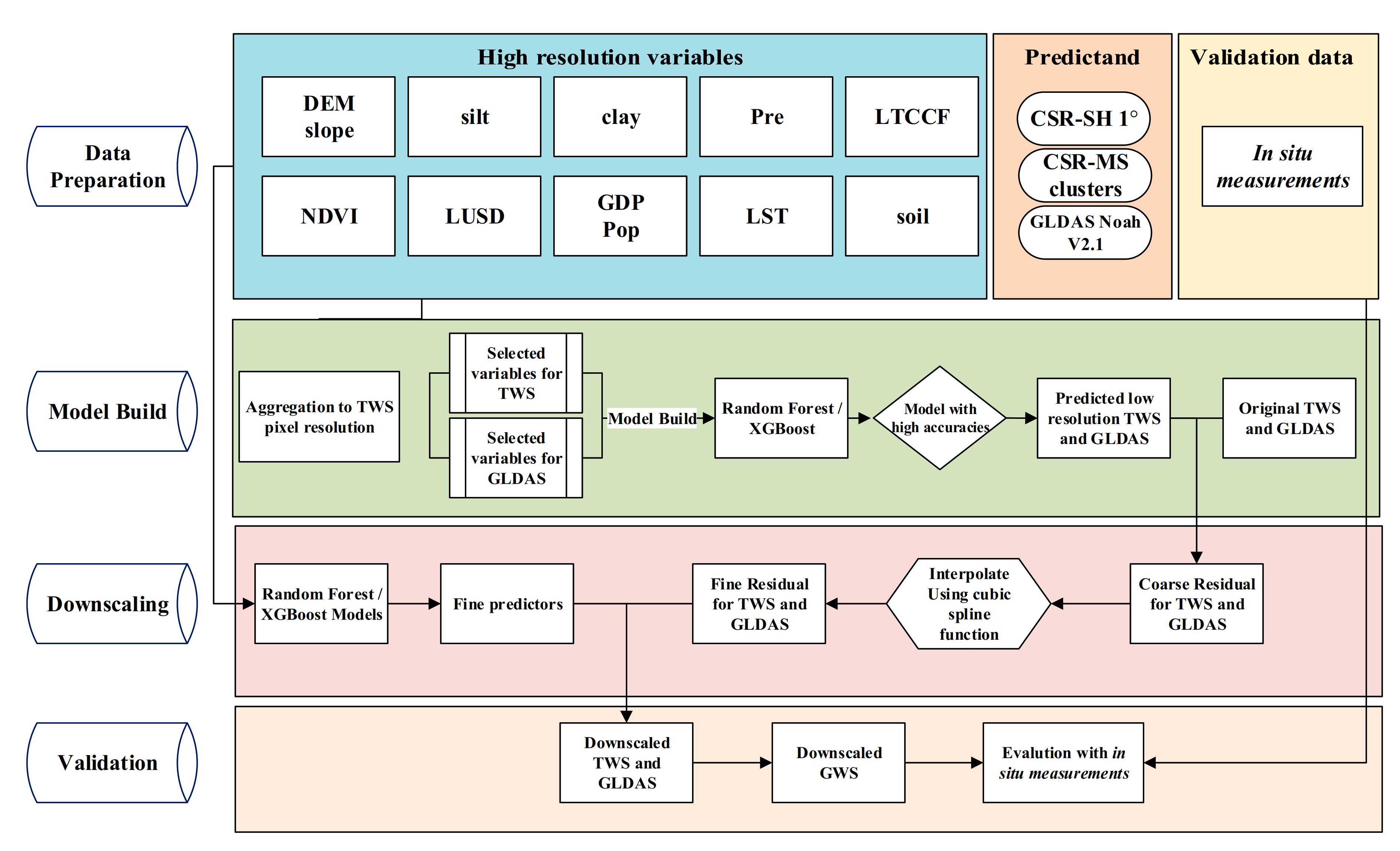
3.1. Technical Route
The approach for downscaling is shown in Figure 1. We used a low-resolution dataset to build the model every year from 2004 to 2016 and used high-resolution data to make the predictions. The detailed processes were as follows:
(1) Data Preparation: We prepared two targets—TWS change and GLDAS change data, validation data (in situ measurements) and 1-km high-resolution variables that either directly or indirectly influenced the targets. The fine predictors were aggregated into coarse predictors to be identical to the target variables according to the pixel size of the TWS resolution (i.e., for each predictor, the average value and mode in each pixel were used for the numerical and categorical predictors, respectively) after transferring the GRACE data from the geographic coordinate system to the projection coordinate system.
(2) Model Construction: We constructed the RF and XGBoost models separately according to the data of each year by selecting the proper variables above for TWS and GLDAS. We used the 2010 data, however, when the corresponding variables for given years were missing, including the silt, clay, DEM and slope, the other predictors changed according to the corresponding year. Once we determined the model, we obtained the trained model output at a low resolution and compared it with the original dataset to calculate the residual.
(3) Downscaling: The residuals were interpreted as the natural random variations that cannot be explained by the existing models [60]. The coarse residuals were downscaled using a cubic spline function, which is commonly used to deal with the coarse residual when performing machine-learning-based downscaling [34,60,61]. After the prediction, the residual was employed to correct the final 1-km predictand by adding it to the predicted results.
(4) Validation: Finally, the in situ measurements were used to verify the downscaled products by comparing the CCs of the time series.
3.2. Random Forest
The RF is a supervised learning algorithm and a combination of tree predictors such that each decision tree was built using a bootstrap data set and only considers a random subset of variables at each step, which would result in a variety of trees we called RF after do this hundreds of times [62,63]. Each decision tree in RF are run in parallel and there is no interaction between the trees. The algorithm works well for both regression and classification. RF is not sensitive to collinearity. RF “spreads” the variable importance across all the variables [64]. These correlated variables can be evaluated to have similar variable importance [65]. This is very valuable in modeling, especially for a complex, nonlinear system because it is commonly difficult to decide which variable to remove when two (or more) variables correlate with each other [66]. In this study, we use RF to build a regression model for the quantitative prediction of TWS and GLDAS. As mentioned in technical route above, there are 966 grids data in China according to the TWS resolution and 15,363 grids data according to GLDAS resolution. For each grid, our targets are GLDAS and TWS, and these 12 variables are important for model building of GLDAS while 9 of them are sufficient to predict the characteristics of TWS based on model accuracy and importance ranking of variables. Every grid with the predictors and target is one sample and we have 966 samples for TWS and 15,363 samples for GLDAS throughout China. We randomly selected training set and testing set according to the ratio of 7:3. When the selected variables were put into the model, all the trees in RF were run independently and the result of model prediction was the average value of all trees generated. The hyper-parameters of the RF in this study were set to the defaults using the “randomForest” package of R language [67]. The R2 and root-mean-square error (RMSE) metrics were used to evaluate the performance of the model. After selecting the optimal model, we brought the 1-km resolution predictors into it to predict the downscaling result. After adding the residuals to predict the result, we got the final downscaled TWS and GLDAS.
3.3. Extreme Gradient Boosting (XGBoost)
XGBoost is also an ensemble learning technique but it is based on gradient boosting decision tree algorithm. Gradient boosting is an approach in which new models are created that predict the residuals or errors of prior models and are then added together to make the final prediction [68]. XGBoost also needs to construct many decision trees but all the trees are dependent, and each new tree is based on the newest residuals or errors of the prior tree. The predicted value of each sample is the sum of the values of leaves in each tree. Similar to RF, XGBoost can deal with complex nonlinearity relationships and handle the multi-collinearity effect with high accuracy and multi-collinearity didn’t matter in XGBoost [69,70,71]. In our study, the predictors we used were the same as those employed in the RF. We also built the model based on 966 samples for TWS and 15,363 samples for GLDAS across China and randomly selected training set and testing set according to the ratio of 7:3. We optimized the models according to the RMSE and R2 derived from training set and the testing set by adjusting the parameter “nrounds” etc. to control the overfitting. Moreover, we used one-hot encoding [72] to transform the categorical data into dummy variables; the purpose was to transform each categorical feature value into a binary feature value (0 or 1) because the values of categorical variables cannot be recognized in XGBoost when we performed regression analysis. We used the XGBoost package in R [68] and most paremeters were set to the default except that parameter “max_depth” was tuned from 6 to 10 and parameter “nrounds” was tuned from 20 to 50 following the changes of “max_depth” to avoid overfitting according to the root-mean-square error (RMSE) of the training and testing dataset. Finally, we used the selected optimal XGBoost model of each year to predict 1-km-resolution TWS and GLDAS. All the package or tools we used were from “xgboost” package in R language [73].
3.4. Derived GWS
The downscaled GRACE data were combined with the downscaled GLDAS data to derive the GWS. We used a vertical water model [9,74] to derive the GWS and compared it with the in situ measurements. The GWS can be calculated according to Equation (1):
where SWS, SWE and CWS were obtained from GLDAS Noah V2.1 and the anomalies were calculated relative to the same baseline time period with GRACE (2004–2009). is the scaling factor [75] and was downscaled to 1 km using cubic convolution before equation (1) was used. Because accurate lake, river, and reservoir data for all of China are not available, we ignored the contributions of these data in our study [6].
3.5. Mean Shift Clustering Analysis
As the CSR-MS products are estimated in irregular (not rectangular) grids of 1 arc degree and spatially interpolated into 0.25 × 0.25 degrees, the values of the spatially interpolated pixels (in 0.25 × 0.25 degrees) do not represent the actual TWS values of those points on earth since there are significant contributions from the geophysical signals of the adjacent pixels. Therefore, we need to restore the native resolution by performing cluster analysis according to the time series [13]. In this study, we used the mean shift clustering approach to identify the optimum number and distribution of clusters of contiguous pixels of similar geophysical signals (GRACE TWS time series). Mean shift clustering is a non-parametric and centroid based clustering method and does not depend on any explicit assumptions about the point distribution, the number of clusters or random initialization when comparing it with the K-means clustering algorithm. The basic idea of this algorithm is to detect the mean points in the densest area and group points based on those mean centers [76].
3.6. Model Evaluation Metrics
The RF model and XGBoost model were evaluated using R2, CC, and RMS. R2 is a statistical measure that represents the proportion of the variance for a dependent variable explained by the independent variables in the regression model. The CC was used to measure the correlation between two variables, and the RMSE was used to measure the error between two datasets. The three metrics are computed as shown in Equations (2)–(4), respectively:
where represents the observations; represents the predicted values; denotes the number of testing data; and and are the mean values of and , respectively.
4. Results
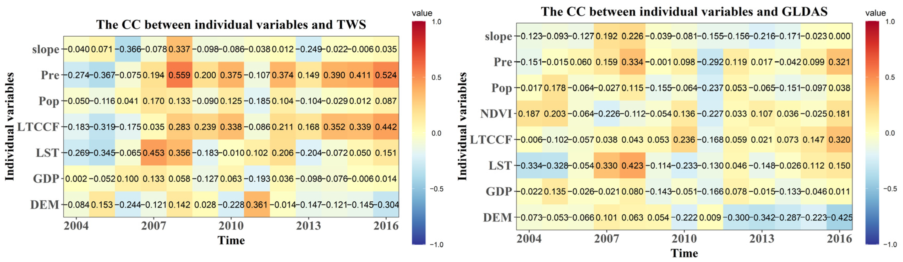
4.1. The Correlation Coefficient between Individual Variables and Targets
Figure 2 showed the scatter plots and CC between the numerical variables and the target variables. Each box represents the CC between predictors and the target variable and the values are also marked. Positive correlations are shown in red and negative correlations are shown in blue. The results show that CC ranged from −0.367–0.559 for TWS and −0.425–0.423 for GLDAS. The highest CC compared with TWS was the precipitation in 2008, with a CC of 0.559. The highest CC compared with GLDAS was DEM in 2016, with a correlation coefficient of −0.425.
4.2. Model Accuracies
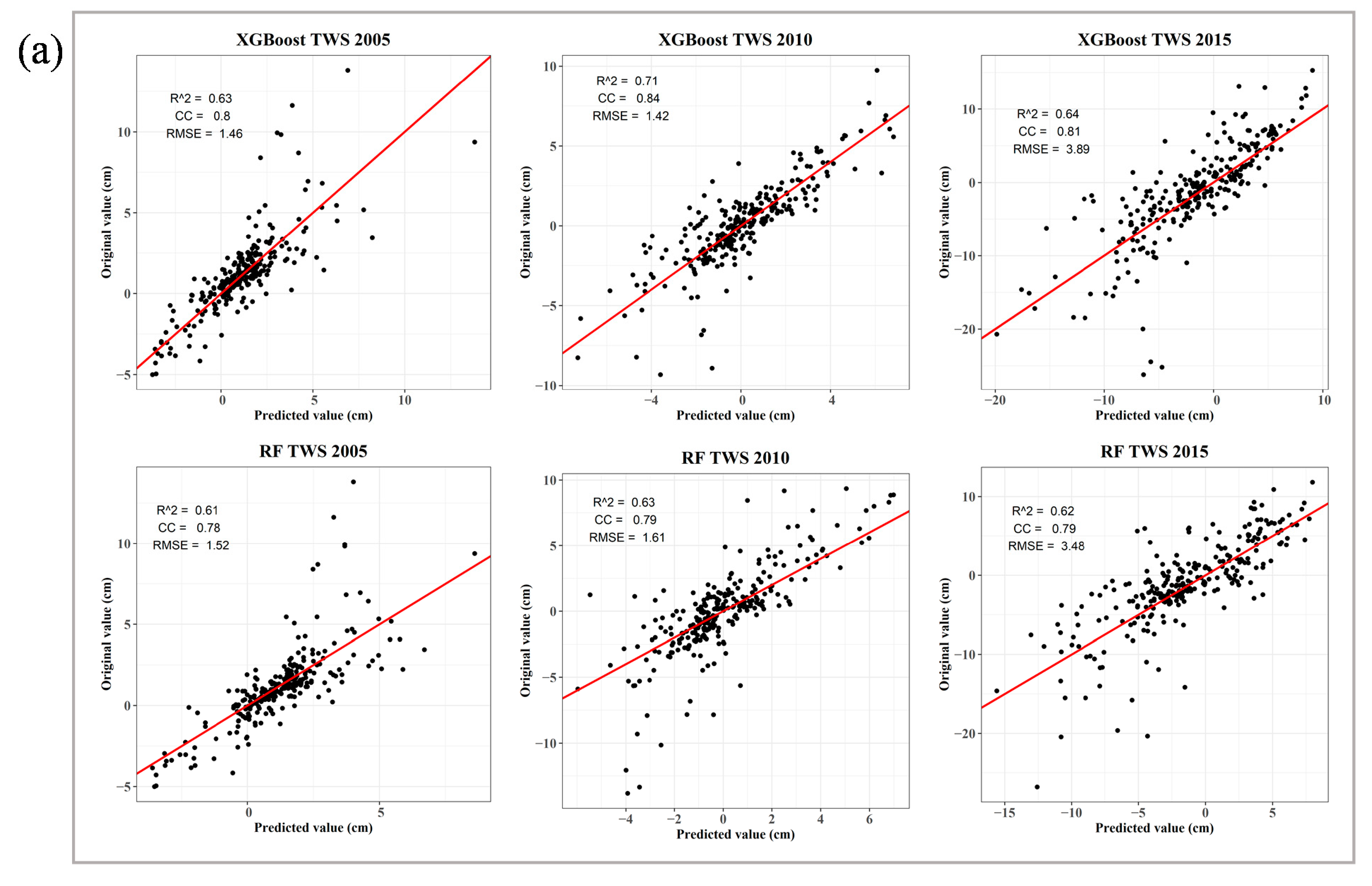
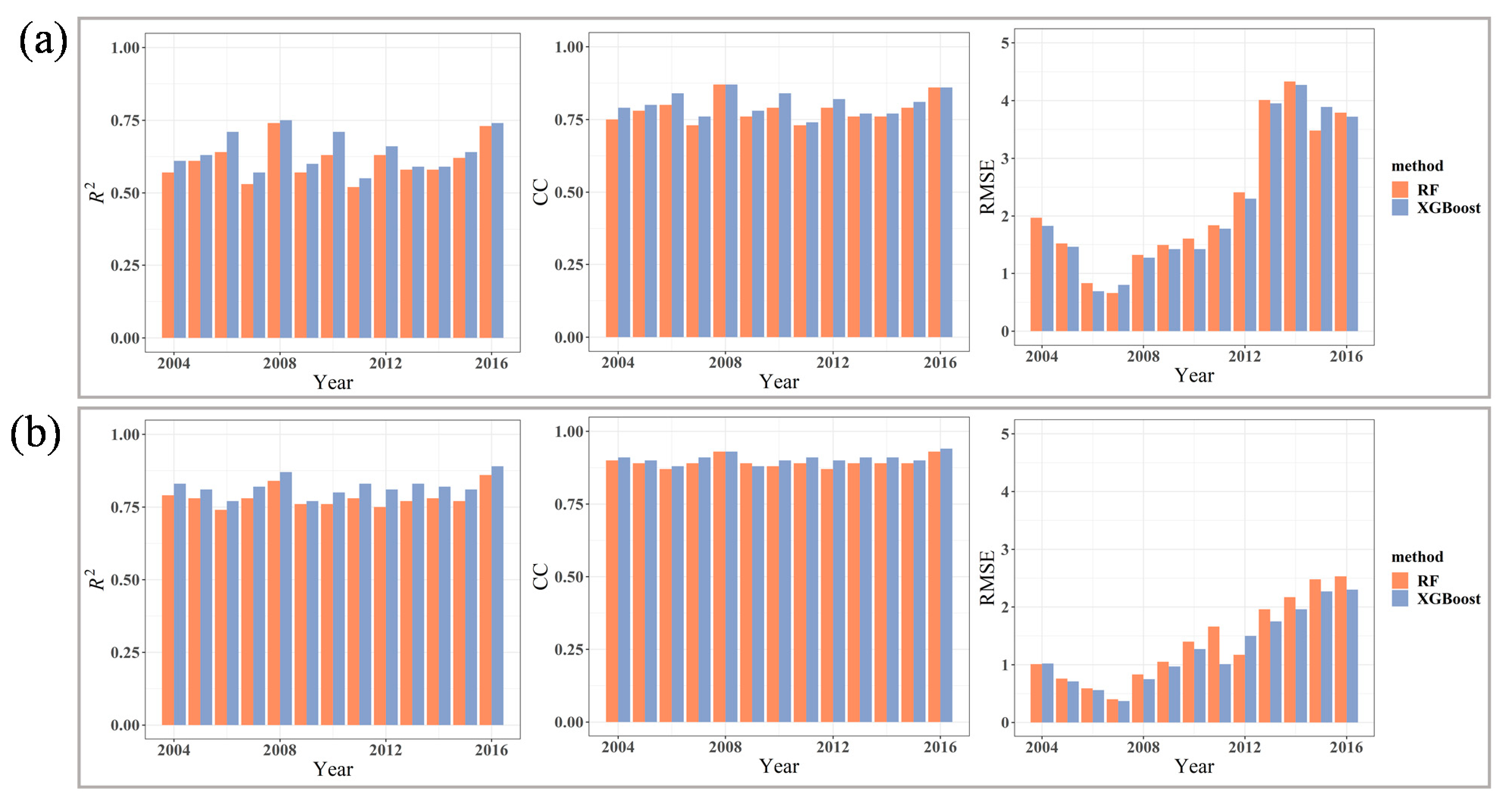
We obtained 906 clusters based on CSR-MS data using mean shift clustering analysis (Figure S3) and then we constructed XGBoost and RF models based on CSR-MS 906 cluster and CSR-SH data. Figure 3 shows the scatterplots and regression fits of the testing dataset of TWS between the predicted values (X-axis) and original values (Y-axis) using the XGBoost and RF methods for the 2005, 2010 and 2015 (the results of other years are given in the supplementary file, Figures S4–S6 and S8), and the results of the evaluation metrics of each year are shown in Figure 4. The R2 accuracy of the XGBoost model ranged from 0.55 to 0.75, the CC ranged from 0.74 to 0.87 and the RMSE ranged from 0.8 to 4.27, while the R2, CC and RMSE had ranges of 0.52–0.74, 0.73–0.87 and 0.66–4.33 respectively, for the RF model when using 906 clusters to construct the regression models in Figure 4a. While the R2, CC and RMSE based on XGBoost ranged from 0.77–0.89 (0.74–0.86 for RF), 0.88–0.94 (0.88–0.93 for RF) and 0.37–2.3 (0.4–2.53 for RF), respectively, based on CSR-SH data in Figure 4b. Obviously, the model accuracies based on CSR-SH data are higher than that based on CSR-MS clusters from the comparison above. The CSR-SH data and related regression models were therefore chosen for downscaling process.
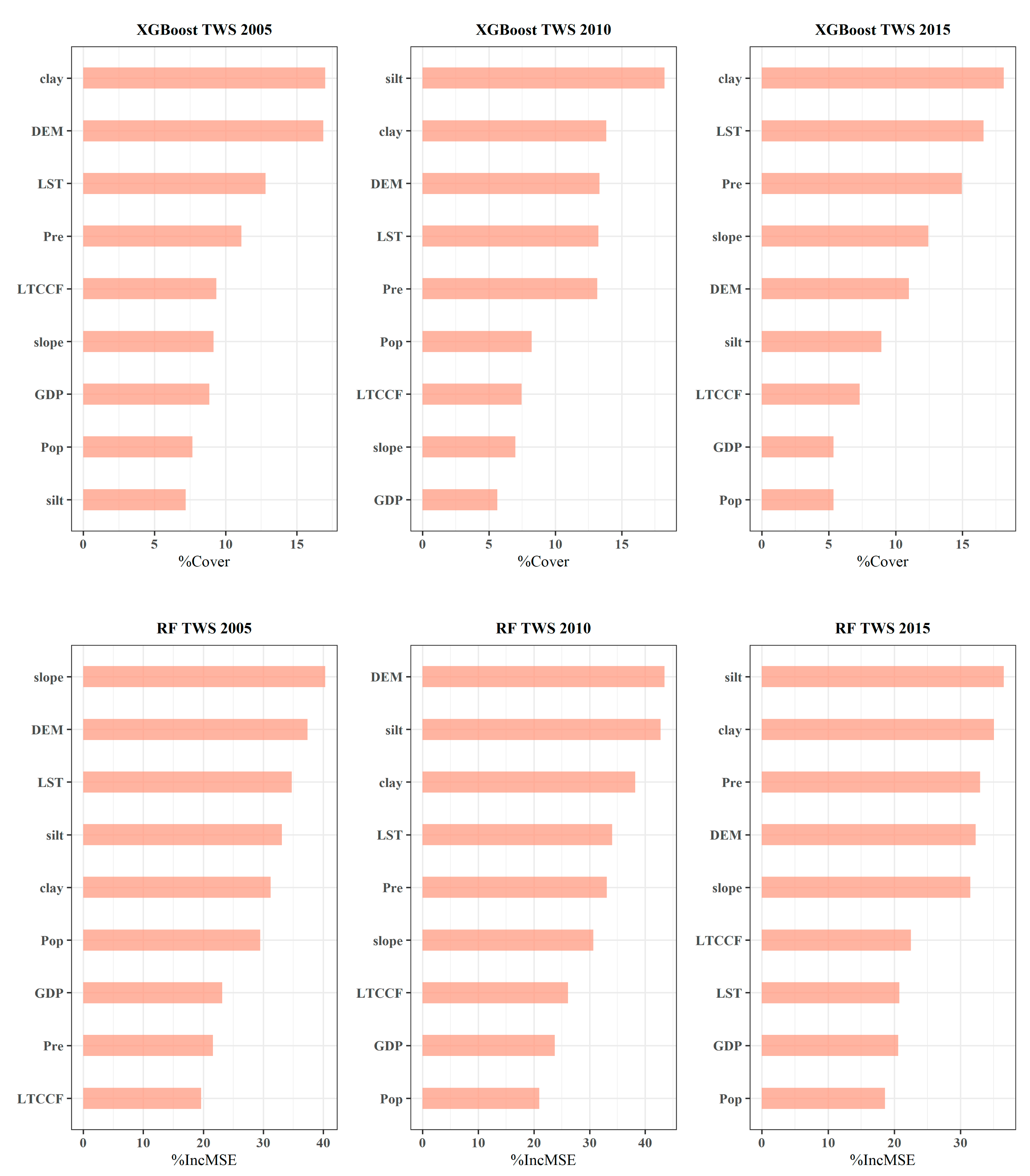
We further analyze the importance of the variables given by the regression models of CSR-SH products, thereby evaluating the predictive ability of the variables. In Figure 5, we show the ranking of importance of variables given by XGBoost-based and RF-based models for 2005, 2010 and 2015 (the results for the other years can be found in the supplementary file, Figures S7 and S9). Comparing the importance of variables given by XGBoost-based and RF-based model, although the rankings calculated by the two methods are slightly different, we can find three variables in common that predominantly influence the TWS, which are precipitation, DEM and clay. They all ranked in the top six except precipitation ranked eighth in 2005 based on RF and clay ranked eighth in 2011 based on XGBoost. Undoubtedly, precipitation plays an important role in replenishing the GWS [6] and TWS [77]. As one of the important influencing factors, DEM determines the recharge and discharge areas of GWS, and is an important input component of groundwater model [78,79,80]. Water-holding capacity is controlled primarily by soil texture and organic matter. Soil with a high percentage of silt and clay particles which describes fine soil has a higher water-holding capacity. Soil textural differences may strongly modify the impact of climate on regional water balance [81].
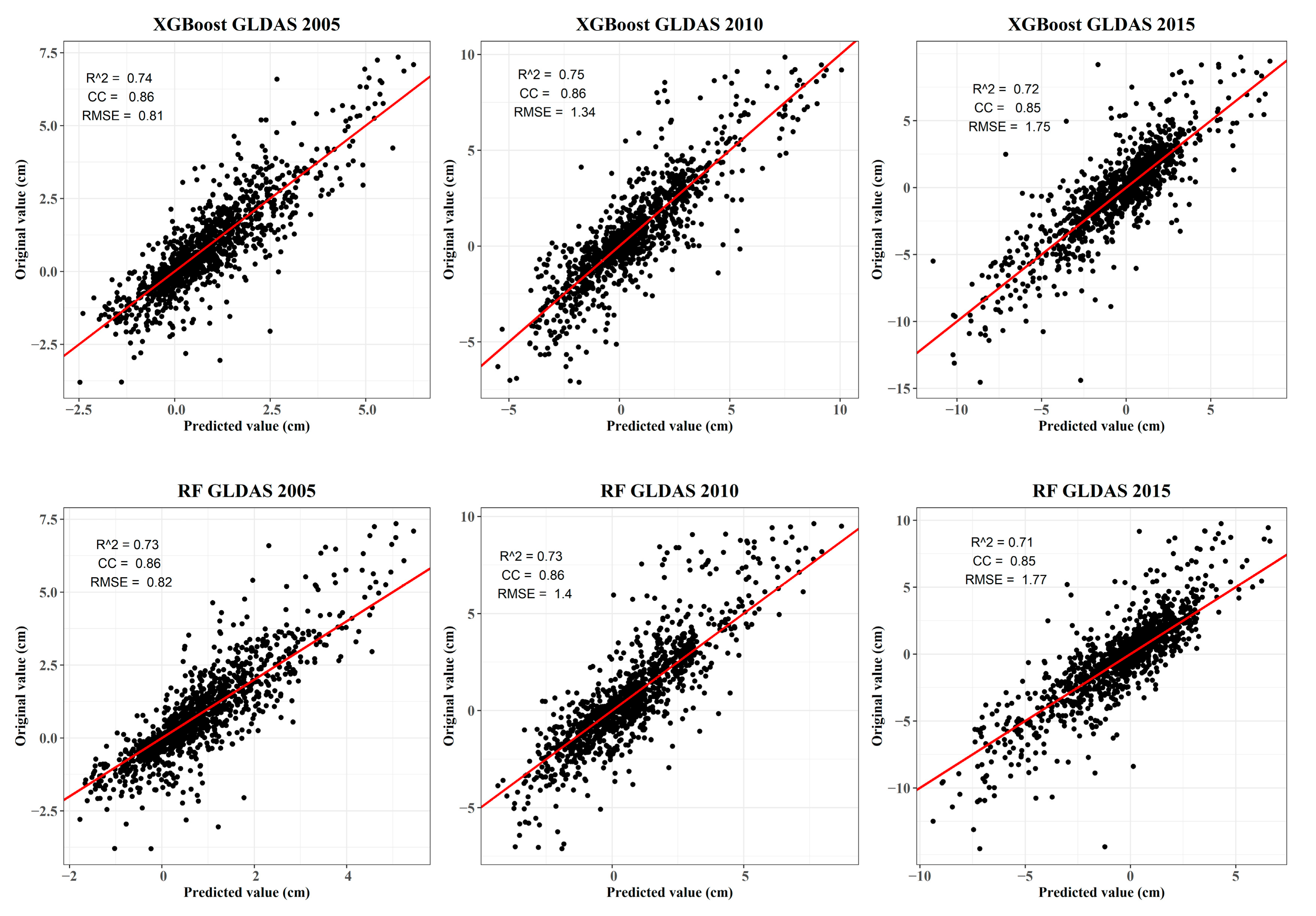
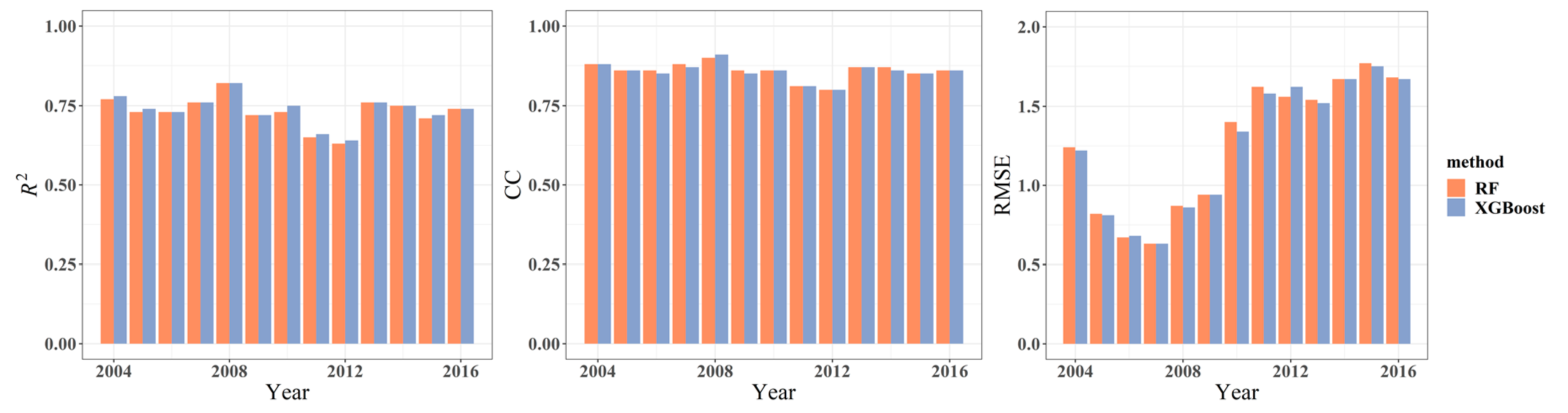
Figure 6 shows the scatterplots and regression fits of the downscaled GLDAS (i.e., the sum of SWE, SMS and CWS) data using the XGBoost and RF models and the original dataset for 2005, 2010 and 2015 (the results of other years are also given in the supplementary file, Figures S10 and S12). These plots demonstrate good agreement between the predicted and original datasets. Figure 7 shows the evaluation metrics of the XGBoost- and RF-based models for the GLDAS from 2004 to 2016. The R2 accuracy of the XGBoost model ranged from 0.64 to 0.82, the CC ranged from 0.80 to 0.91 and the RMSE ranged from 0.63 to 1.75, while the R2, CC and RMSE had ranges of 0.63–0.82, 0.80–0.90, 0.63–1.77 respectively, for the RF model. The highest R2 and CC were reached for 2008, with values of 0.82 (R2) and 0.91 (CC) for the XGBoost model and 0.82 (R2) and 0.90 (CC) for the RF model. The overall correlation was strong, but the overall dispersion degree was higher than that of the TWS. Moreover, both R2 and RMSE accuracies of XGBoost models were better than that of RF models in all years.
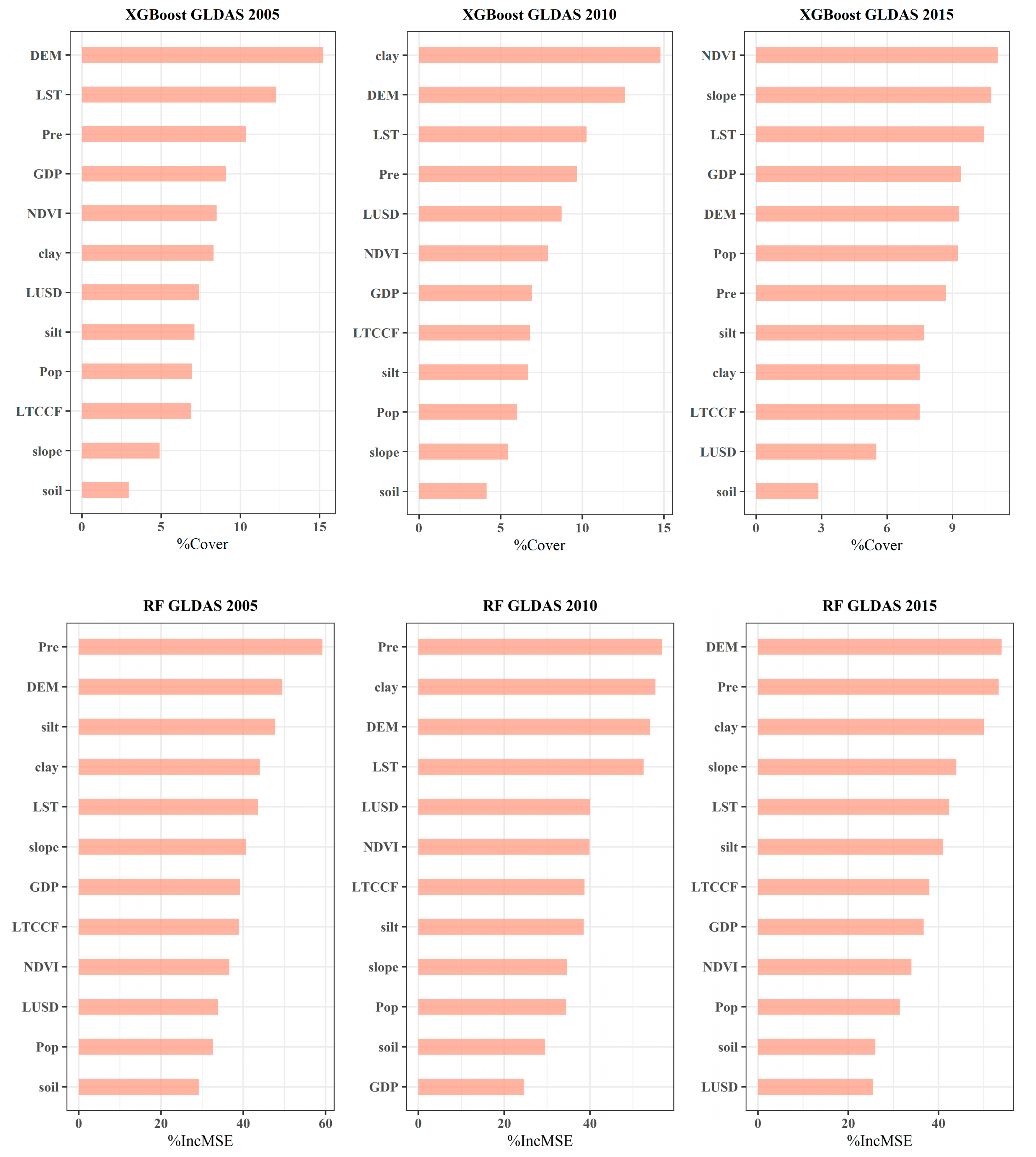
Figure 8 shows plots of the variable importance measure for the XGBoost- and RF-modeled GLDAS for 2005, 2010 and 2015 (the results of other years are also given in the supplementary file, Figures S11 and S13). Comparing the importance of variable given by XGBoost-based and RF-based model, the DEM and precipitation always ranked in the top six except that precipitation ranked seventh in 2012 based on RF. There were 10 years during which the importance of LST ranked in the top six. Other categorical variables, such as clay, also exerted significant influences (within the top six) among 8 years.
Considering the higher accuracy of the XGBoost models, further analysis was performed based on the XGBoost results. However, we provided both downscaled products as supplementary data.
4.3. The Downscaled GWS Analysis
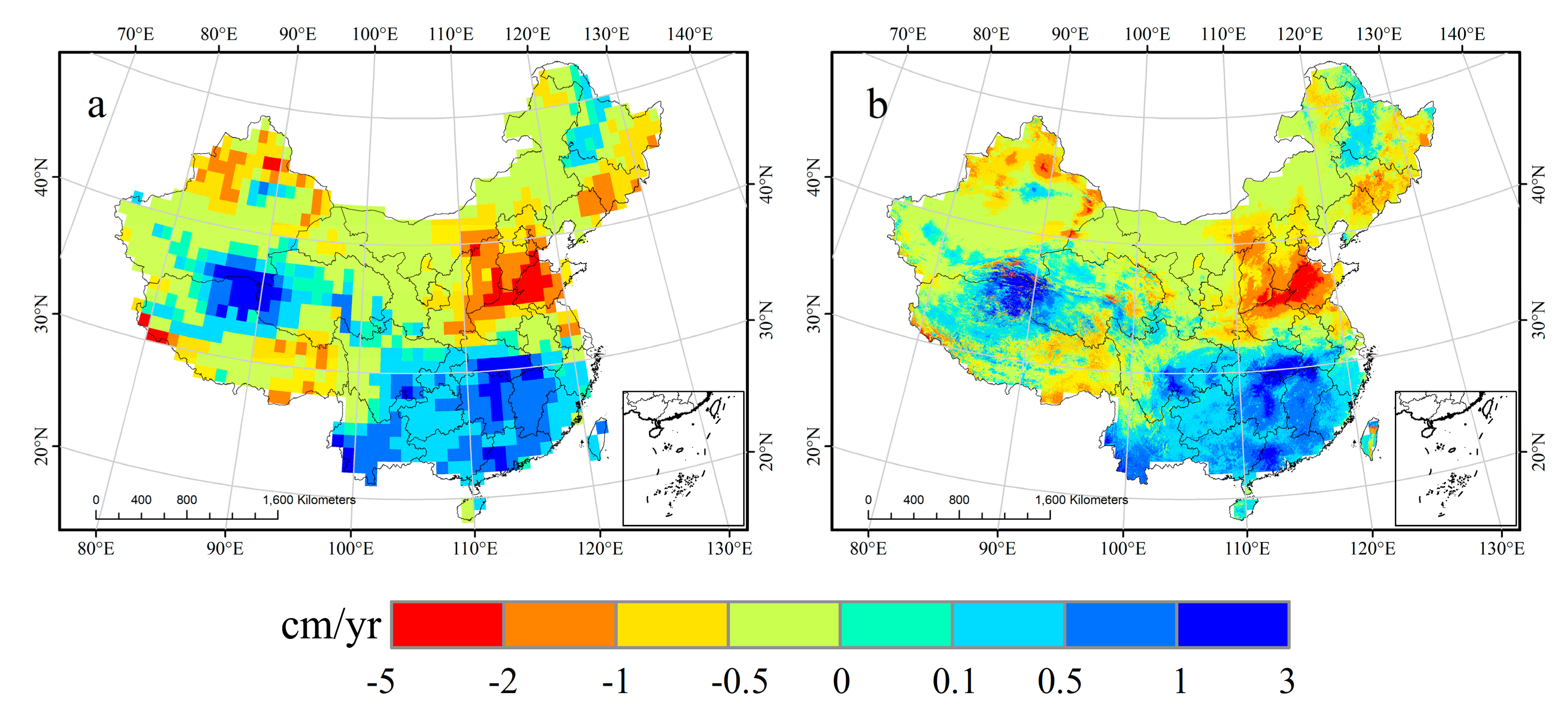
Based on the GRACE CSR-SH and GLDAS data using XGBoost models, we substituted 1 km predictors to obtain the TWS and GLDAS with 1 km resolution and further derived GWS with a resolution of 1 km. Figure 9 shows the interannual variation of GWS derived from the original GWS and downscaled GWS for 2004–2016 based on Thiel-Sen’s slope method [82,83]. Spatially, the overall trends of the original and downscaled GWS are similar: the GWS declined in the North China Plain (NCP) and the northwest but increased in the northeast, southeast and on the Qinghai-Tibet Plateau. The downscaling products were able to reflect area texture information better than the original data, and details were more prominent.
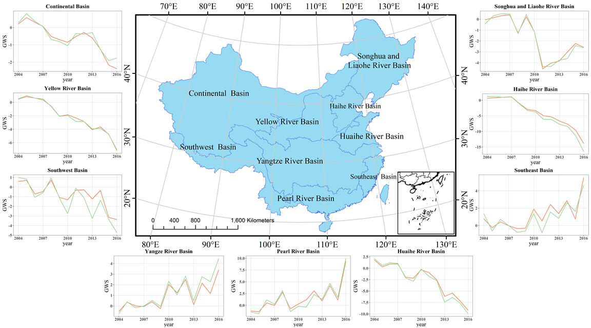
We also evaluated the annual change between the original GWS and XGBoost-downscaled GWS in China in 9 river basins: Songhua and Liaohe River Basin (LRB), Continental Basin (CB), Haihe River Basin (HRB), Huaihe River Basin (HHRB), Southwest Basin (SWB), Southeast Basin (SEB), Yangtze River Basin (YZRB), Pearl River Basin (PRB), and Yellow River Basin (YRB) [84]. Figure 10 shows the distribution of main river basins throughout China and depicts the interannual changes using line charts. The GWS was consistent among all the basins between pre- and post-downscaling. The CC in different basins was 0.929~0.999, and the highest CC was in the HRB while the lowest CC was in the SWB. Among them, five basins (CB, HRB, HHRB, YRB, SWB) showed an overall downward trend while three (YZRB, SEB, PRB) basins showed an overall upward trend in GWS and the three rising regions were located in southeast China. The groundwater in the SLRB basin experienced a sharp decline from 2009 to 2011, and it began to rise gradually after 2011. The CCs between the pre- and post-downscaling products were particularly high, indicating that the downscaled data almost completely maintained the interannual fluctuation characteristics of the original data, verifying that the downscaled products could contain interannual signal characteristics.
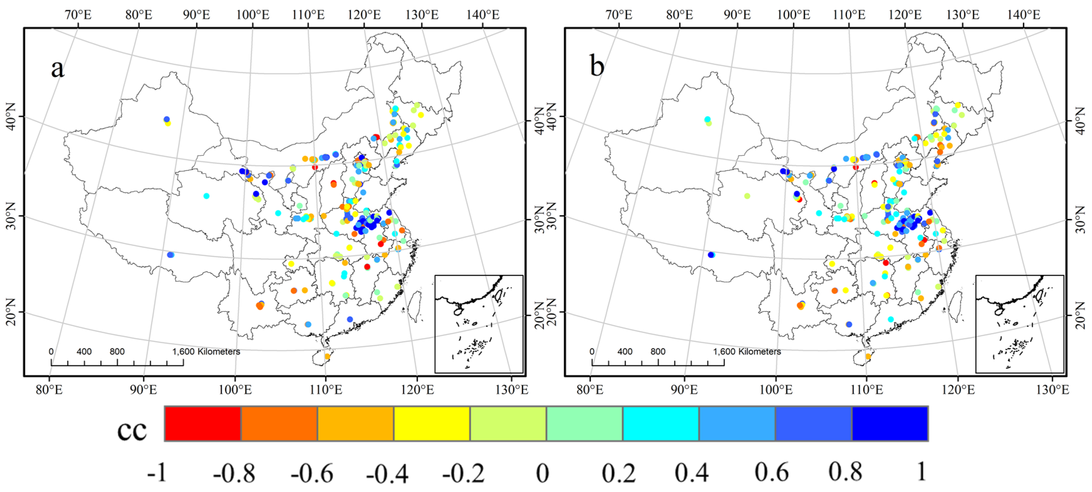
We also calculated the correlations between the in situ measurements and GWS both before and after downscaling, and the results are shown in Figure 11. A similar spatial CC pattern is observed before and after downscaling. There are 69 stations whose CCs were greater than 0.5 before downscaling and 69 stations after downscaling. The downscaled products maintained the accuracy of the original data.
5. Conclusions and Discussion
To compensate for the lack of fine resolution GWS products, this study successfully used machine learning methods to downscale GRACE and GLDAS data in China from 1° and 0.25°, respectively, to a final resolution of 1 km. We ultimately provided time series of downscaled TWS, GLDAS and GWS, which facilitated the evaluation of local GWS changes.
The CCs between the downscaled results given by both models and original data were generally larger than 0.8. The comparison between in situ measurement data from monitoring stations confirmed that the downscaled products maintained the accuracy of the original data. Regarding the spatial distribution, post-downscaled GWS owned higher resolution than pre-downscaled GWS and contained the spatial patterns of the pre-downscaled GWS throughout China. This finding means that these products could be used for the analysis of interannual trends at the local scale. Moreover, a comparison of innerannual changes based on 9 river basins between the pre- and post-downscaling GWS also emphasized the reliability of the downscaled products.
Accurate products bring higher-resolution data support for various GRACE-related researches in the later period. For example, the detailed TWS and GWS data provide support for the input data of the regional hydrological models with a resolution of 1 km. At the same time, it provides a dataset for verification and revision of the model parameters combined with the groundwater output from the regional hydrological models. In addition, this dataset makes the use of GRACE data and InSAR-based technic analysis to evaluate the relationship between groundwater consumption and ground subsidence more scientific and effective. Finally, accurate GWS and TWS contribute to land use, city planning and water resources management. The 1 km resolution products can effectively provide the dynamics of regional water resources change and provide data support for managers’ policy formulation like balancing the relationship between regional irrigation water use and groundwater consumption.
There are still some limitations in this analysis. First, the downscaling predictors were not free from error, so we could not evaluate the total error in this study. Second, the number of in situ measurements used for verification was only 251, and their spatial distribution was uneven. Including additional data from monitoring stations would make the results more meaningful. Third, the coarse residuals of TWS and GLDAS were resampled using cubic spline interpolation and the inter-pixel changes should be further considered. Finally, due to the lack of accurate data on lakes, rivers, and reservoirs for all of China, we ignored the contributions from these sources when performing the comparison with in situ measurements. Nevertheless, our produced high-resolution data can provide certain guidelines for detailed investigations of the regional GWS and can help improve future hydrological research on small scales and local areas, thereby enhancing the capability for sustainable water resources management.
The 1 km resolution data of TWS, GWS and GLDAS in this paper can be found at Supplementary Materials.
Supplementary Materials
The Supplementary Material is available online at https://0-www-mdpi-com.brum.beds.ac.uk/2072-4292/13/3/523/s1 and https://zenodo.org/record/4521973#.YCJW5iMRVPY.
Author Contributions
Conceptualization, K.L., M.W.; methodology, J.Z., K.L., and M.W.; validation, J.Z. and K.L.; formal analysis, J.Z. and K.L.; investigation, J.Z., K.L., and M.W.; resources, J.Z.; data curation, J.Z. and K.L.; writing—original draft preparation, J.Z.; writing—review and editing, K.L.; visualization, J.Z. and K.L.; supervision, K.L.; project administration, K.L.; funding acquisition, K.L. All authors have read and agreed to the published version of the manuscript.
Funding
This research was funded by National Natural Science Foundation of China (41771538), National Key Research and Development Plan (2017YFC1502901) and Beijing Municipal Science and Technology Project (Z181100009018009).
Acknowledgments
The research for this article was supported by the National Natural Science Foundation of China (41771538), National Key Research and Development Plan (2017YFC1502901) and Beijing Municipal Science and Technology Project (Z181100009018009). The financial support is highly appreciated. There is no conflict of interest to declare. We would like to thank the high-performance computing support from the Center for Geodata and Analysis, Faculty of Geographical Science, Beijing Normal University (https://gda.bnu.edu.cn/). We thank Yulong Zhong for his insightful suggestions. Meanwhile, we thank two anonymous reviewers for their insightful comments, which help us to improve this paper.
Conflicts of Interest
The authors declare no conflict of interest.
References
- Cosgrove, W.J.; Loucks, D.P. Water management: Current and future challenges and research directions. Water Resour. Res. 2015, 51, 4823–4839. [Google Scholar] [CrossRef] [Green Version]
- de Graaf, I.D.; Sutanudjaja, E.; Van Beek, L.; Bierkens, M. A high-resolution global-scale groundwater model. Hydrol. Earth Syst. Sci. 2015, 19, 823–837. [Google Scholar] [CrossRef] [Green Version]
- Wada, Y.; Wisser, D.; Bierkens, M.F. Global modeling of withdrawal, allocation and consumptive use of surface water and groundwater resources. Earth Syst. Dyn. Discuss. 2014, 5, 15–40. [Google Scholar] [CrossRef] [Green Version]
- Scanlon, B.R.; Zhang, Z.; Save, H.; Sun, A.Y.; Schmied, H.M.; Van Beek, L.P.; Wiese, D.N.; Wada, Y.; Long, D.; Reedy, R.C. Global models underestimate large decadal declining and rising water storage trends relative to GRACE satellite data. Proc. Natl. Acad. Sci. USA 2018, 115, E1080–E1089. [Google Scholar] [CrossRef] [Green Version]
- Chen, J.; Famigliett, J.S.; Scanlon, B.R.; Rodell, M. Groundwater storage changes: Present status from GRACE observations. Surv. Geophys. 2016, 37, 397–417. [Google Scholar] [CrossRef]
- Zhang, J.; Liu, K.; Wang, M. Seasonal and Interannual Variations in China’s Groundwater Based on GRACE Data and Multisource Hydrological Models. Remote Sens. 2020, 12, 845. [Google Scholar] [CrossRef] [Green Version]
- Aeschbach-Hertig, W.; Gleeson, T. Regional strategies for the accelerating global problem of groundwater depletion. Nat. Geosci. 2012, 5, 853–861. [Google Scholar] [CrossRef]
- Li, B.; Rodell, M.; Kumar, S.; Beaudoing, H.K.; Getirana, A.; Zaitchik, B.F.; de Goncalves, L.G.; Cossetin, C.; Bhanja, S.; Mukherjee, A. Global GRACE data assimilation for groundwater and drought monitoring: Advances and challenges. Water Resour. Res. 2019, 55, 7564–7586. [Google Scholar] [CrossRef] [Green Version]
- Long, D.; Chen, X.; Scanlon, B.R.; Wada, Y.; Hong, Y.; Singh, V.P.; Chen, Y.; Wang, C.; Han, Z.; Yang, W. Have GRACE satellites overestimated groundwater depletion in the Northwest India Aquifer? Sci. Rep. 2016, 6, 24398. [Google Scholar] [CrossRef]
- Scanlon, B.R.; Longuevergne, L.; Long, D. Ground referencing GRACE satellite estimates of groundwater storage changes in the California Central Valley, USA. Water Resour. Res. 2012, 48, 48. [Google Scholar] [CrossRef] [Green Version]
- Rodell, M.; Houser, P.; Jambor, U.; Gottschalck, J.; Mitchell, K.; Meng, C.-J.; Arsenault, K.; Cosgrove, B.; Radakovich, J.; Bosilovich, M. The global land data assimilation system. Bull. Am. Meteorol. Soc. 2004, 85, 381–394. [Google Scholar] [CrossRef] [Green Version]
- Chen, J.; Rodell, M.; Wilson, C.; Famiglietti, J. Low degree spherical harmonic influences on Gravity Recovery and Climate Experiment (GRACE) water storage estimates. Geophys. Res. Lett. 2005, 32, 32. [Google Scholar] [CrossRef] [Green Version]
- Sahour, H.; Sultan, M.; Vazifedan, M.; Abdelmohsen, K.; Karki, S.; Yellich, J.A.; Gebremichael, E.; Alshehri, F.; Elbayoumi, T.M. Statistical applications to downscale GRACE-derived terrestrial water storage data and to fill temporal gaps. Remote Sens. 2020, 12, 533. [Google Scholar] [CrossRef] [Green Version]
- Du, Z.; Ge, L.; Ng, A.H.-M.; Li, X. Time series interferometry integrated with groundwater depletion measurement from GRACE. In Proceedings of the 2016 IEEE International Geoscience and Remote Sensing Symposium (IGARSS), Beijing, China, 10–15 July 2016; pp. 1166–1169. [Google Scholar]
- Gong, H.; Pan, Y.; Zheng, L.; Li, X.; Zhu, L.; Zhang, C.; Huang, Z.; Li, Z.; Wang, H.; Zhou, C. Long-term groundwater storage changes and land subsidence development in the North China Plain (1971–2015). Hydrogeol. J. 2018, 26, 1417–1427. [Google Scholar] [CrossRef] [Green Version]
- Zhou, C.; Gong, H.; Chen, B.; Zhu, F.; Duan, G.; Gao, M.; Lu, W. Land subsidence under different land use in the eastern Beijing plain, China 2005–2013 revealed by InSAR timeseries analysis. Gisci. Remote Sens. 2016, 53, 671–688. [Google Scholar] [CrossRef]
- Li, J.; Wang, S.; Michel, C.; Russell, H.A. Surface deformation observed by InSAR shows connections with water storage change in Southern Ontario. J. Hydrol. Reg. Stud. 2020, 27, 100661. [Google Scholar] [CrossRef]
- Castellazzi, P.; Martel, R.; Rivera, A.; Huang, J.; Pavlic, G.; Calderhead, A.I.; Chaussard, E.; Garfias, J.; Salas, J. Groundwater depletion in Central Mexico: Use of GRACE and InSAR to support water resources management. Water Resour. Res. 2016, 52, 5985–6003. [Google Scholar] [CrossRef]
- Zheng, M.; Deng, K.; Fan, H.; Du, S. Monitoring and analysis of surface deformation in mining area based on InSAR and GRACE. Remote Sens. 2018, 10, 1392. [Google Scholar] [CrossRef] [Green Version]
- Guo, J.; Zhou, L.; Yao, C.; Hu, J. Surface subsidence analysis by multi-temporal insar and grace: A case study in Beijing. Sensors 2016, 16, 1495. [Google Scholar] [CrossRef] [Green Version]
- Castellazzi, P.; Longuevergne, L.; Martel, R.; Rivera, A.; Brouard, C.; Chaussard, E. Quantitative mapping of groundwater depletion at the water management scale using a combined GRACE/InSAR approach. Remote Sens. Environ. 2018, 205, 408–418. [Google Scholar] [CrossRef]
- Zaitchik, B.F.; Rodell, M.; Reichle, R.H. Assimilation of GRACE terrestrial water storage data into a land surface model: Results for the Mississippi River basin. J. Hydrometeorol. 2008, 9, 535–548. [Google Scholar] [CrossRef]
- Sahoo, A.K.; De Lannoy, G.J.; Reichle, R.H.; Houser, P.R. Assimilation and downscaling of satellite observed soil moisture over the Little River Experimental Watershed in Georgia, USA. Adv. Water Resour. 2013, 52, 19–33. [Google Scholar] [CrossRef]
- Shokri, A.; Walker, J.P.; van Dijk, A.I.; Pauwels, V.R. On the use of adaptive ensemble Kalman filtering to mitigate error misspecifications in GRACE data assimilation. Water Resour. Res. 2019, 55, 7622–7637. [Google Scholar] [CrossRef] [Green Version]
- Shokri, A.; Walker, J.P.; van Dijk, A.I.; Pauwels, V.R. Performance of different ensemble Kalman filter structures to assimilate GRACE terrestrial water storage estimates into a high-resolution hydrological model: A synthetic study. Water Resour. Res. 2018, 54, 8931–8951. [Google Scholar] [CrossRef]
- Schoof, J.T. Statistical downscaling in climatology. Geogr. Compass 2013, 7, 249–265. [Google Scholar] [CrossRef] [Green Version]
- Majumdar, S.; Smith, R.; Butler, J., Jr.; Lakshmi, V. Groundwater Withdrawal Prediction Using Integrated Multitemporal Remote Sensing Data Sets and Machine Learning. Water Resour. Res. 2020, 56, e2020WR028059. [Google Scholar] [CrossRef]
- Sun, A.; Scanlon, B.; Save, H.; Rateb, A. Reconstruction of GRACE Total Water Storage through Automated Machine Learning. Water Resour. Res. 2020. [Google Scholar] [CrossRef]
- Yan, J.; Jia, S.; Lv, A.; Zhu, W. Water resources assessment of China’s transboundary river basins using a machine learning approach. Water Resour. Res. 2019, 55, 632–655. [Google Scholar] [CrossRef]
- Michael, W.J.; Minsker, B.S.; Tcheng, D.; Valocchi, A.J.; Quinn, J.J. Integrating data sources to improve hydraulic head predictions: A hierarchical machine learning approach. Water Resour. Res. 2005, 41. [Google Scholar] [CrossRef] [Green Version]
- Cho, E.; Jacobs, J.M.; Jia, X.; Kraatz, S. Identifying Subsurface Drainage using Satellite Big Data and Machine Learning via Google Earth Engine. Water Resour. Res. 2019, 55, 8028–8045. [Google Scholar] [CrossRef]
- Seyoum, W.M.; Kwon, D.; Milewski, A.M. Downscaling GRACE TWSA data into high-resolution groundwater level anomaly using machine learning-based models in a glacial aquifer system. Remote Sens. 2019, 11, 824. [Google Scholar] [CrossRef] [Green Version]
- Milewski, A.M.; Thomas, M.B.; Seyoum, W.M.; Rasmussen, T.C. Spatial Downscaling of GRACE TWSA Data to Identify Spatiotemporal Groundwater Level Trends in the Upper Floridan Aquifer, Georgia, USA. Remote Sens. 2019, 11, 2756. [Google Scholar] [CrossRef] [Green Version]
- Chen, L.; He, Q.; Liu, K.; Li, J.; Jing, C. Downscaling of GRACE-Derived Groundwater Storage Based on the Random Forest Model. Remote Sens. 2019, 11, 2979. [Google Scholar] [CrossRef] [Green Version]
- Ning, S.; Ishidaira, H.; Wang, J. Statistical downscaling of GRACE-derived terrestrial water storage using satellite and GLDAS products. Proc. Civ. Eng. Soc. 2014, 70, I_133–I_138. [Google Scholar] [CrossRef]
- Yin, W.; Hu, L.; Zhang, M.; Wang, J.; Han, S.C. Statistical Downscaling of GRACE-Derived Groundwater Storage Using ET Data in the North China Plain. J. Geophys. Res. Atmos. 2018, 123, 5973–5987. [Google Scholar] [CrossRef]
- Rahaman, M.M.; Thakur, B.; Kalra, A.; Li, R.; Maheshwari, P. Estimating High-Resolution Groundwater Storage from GRACE: A Random Forest Approach. Environments 2019, 6, 63. [Google Scholar] [CrossRef] [Green Version]
- Miro, M.E.; Famiglietti, J.S. Downscaling GRACE remote sensing datasets to high-resolution groundwater storage change maps of California’s Central Valley. Remote Sens. 2018, 10, 143. [Google Scholar] [CrossRef] [Green Version]
- Wan, Z.; Zhang, K.; Xue, X.; Hong, Z.; Hong, Y.; Gourley, J.J. Water balance-based actual evapotranspiration reconstruction from ground and satellite observations over the conterminous United States. Water Resour. Res. 2015, 51, 6485–6499. [Google Scholar] [CrossRef]
- Sehler, R.; Li, J.; Reager, J.; Ye, H. Investigating Relationship Between Soil Moisture and Precipitation Globally Using Remote Sensing Observations. J. Contemp. Water Res. Educ. 2019, 168, 106–118. [Google Scholar] [CrossRef] [Green Version]
- Engineers, S.C.; Borchers, J.W.; Carpenter, M.; Grabert, V.K.; Dalgish, B.; Cannon, D. Land Subsidence from Groundwater Use in California; California Water Foundation: Sacramento, CA, USA, 2014. [Google Scholar]
- Qiu, L.; Huang, J.; Niu, W. Decoupling and Driving Factors of Economic Growth and Groundwater Consumption in the Coastal Areas of the Yellow Sea and the Bohai Sea. Sustainability 2018, 10, 4158. [Google Scholar] [CrossRef] [Green Version]
- Lerner, D.N.; Harris, B. The relationship between land use and groundwater resources and quality. Land Use Policy 2009, 26, S265–S273. [Google Scholar] [CrossRef]
- Hazarika, N.; Nitivattananon, V. Strategic assessment of groundwater resource exploitation using DPSIR framework in Guwahati city, India. Habitat Int. 2016, 51, 79–89. [Google Scholar] [CrossRef]
- Jackson, J. Developing regional tourism in China: The potential for activating business clusters in a socialist market economy. Tour. Manag. 2006, 27, 695–706. [Google Scholar] [CrossRef]
- Zaidi, F.K.; Nazzal, Y.; Ahmed, I.; Naeem, M.; Jafri, M.K. Identification of potential artificial groundwater recharge zones in Northwestern Saudi Arabia using GIS and Boolean logic. J. Afr. Earth Sci. 2015, 111, 156–169. [Google Scholar] [CrossRef]
- Pakparvar, M.; Hashemi, H.; Rezaei, M.; Cornelis, W.M.; Nekooeian, G.; Kowsar, S.A. Artificial recharge efficiency assessment by soil water balance and modelling approaches in a multi-layered vadose zone in a dry region. Hydrol. Sci. J. 2018, 63, 1183–1202. [Google Scholar] [CrossRef]
- Mokarram, M.; Shaygan, M.; Sathyamoorthy, D. Using DEM and GIS for evaluation of groundwater resources in relation to landforms in the Maharlou-Bakhtegan watershed, Fars province, Iran. J. Water Land Dev. 2018, 37, 121–126. [Google Scholar] [CrossRef]
- Joffre, R.; Rambal, S. How tree cover influences the water balance of Mediterranean rangelands. Ecology 1993, 74, 570–582. [Google Scholar] [CrossRef]
- Yi, L.; Xiong, L.; Yang, X. Method of pixelizing GDP data based on the GIS. J. Gansu Sci 2006, 18, 54–58. [Google Scholar]
- Liu, H.; Jiang, D.; Yang, X.; Luo, C. Spatialization approach to 1 km grid GDP supported by remote sensing. Geo-Inf. Sci. 2005, 2, 26. [Google Scholar]
- Gandhi, S.M.; Sarkar, B.C. Chapter 3—Reconnaissance and Prospecting. In Essentials of Mineral Exploration and Evaluation; Gandhi, S.M., Sarkar, B.C., Eds.; Elsevier: Amsterdam, The Netherlands, 2016; pp. 53–79. [Google Scholar] [CrossRef]
- Didan, K. MOD13A2 MODIS/Terra Vegetation indices 16-Day L3 Global 1km SIN Grid V006 [Data set]. NASA Eosdis Lp DAAC 2015, 6. [Google Scholar] [CrossRef]
- Wan, Z.; Hook, S.; Hulley, G. MOD11A1 MODIS/Terra Land Surface Temperature/Emissivity Daily L3 Global 1 km SIN Grid V006 [Data Set]; NASA: Washington, DC, USA, 2015. [Google Scholar]
- Sexton, J.O.; Song, X.-P.; Feng, M.; Noojipady, P.; Anand, A.; Huang, C.; Kim, D.-H.; Collins, K.M.; Channan, S.; DiMiceli, C. Global, 30-m resolution continuous fields of tree cover: Landsat-based rescaling of MODIS vegetation continuous fields with lidar-based estimates of error. Int. J. Digit. Earth 2013, 6, 427–448. [Google Scholar] [CrossRef] [Green Version]
- Peng, S.; Ding, Y.; Liu, W.; Li, Z. 1 km monthly temperature and precipitation dataset for China from 1901 to 2017. Earth Syst. Sci. Data 2019, 11, 1931–1946. [Google Scholar] [CrossRef] [Green Version]
- Landerer, F.W.; Swenson, S. Accuracy of scaled GRACE terrestrial water storage estimates. Water Resour. Res. 2012, 48, 48. [Google Scholar] [CrossRef]
- Save, H.; Bettadpur, S.; Tapley, B.D. High-resolution CSR GRACE RL05 mascons. J. Geophys. Res. Solid Earth 2016, 121, 7547–7569. [Google Scholar] [CrossRef]
- China Institute of Geological Environment Monitoring (CIGEM). China Geological Environment Monitoring: Groundwater Yearbook; China Land Press: Beijing, China, 2013. [Google Scholar]
- Fang, J.; Du, J.; Xu, W.; Shi, P.; Li, M.; Ming, X. Spatial downscaling of TRMM precipitation data based on the orographical effect and meteorological conditions in a mountainous area. Adv. Water Resour. 2013, 61, 42–50. [Google Scholar] [CrossRef]
- Fu, Y.; Xu, S.; Zhang, C.; Sun, Y. Spatial downscaling of MODIS Chlorophyll-a using Landsat 8 images for complex coastal water monitoring. Estuar. Coast. Shelf Sci. 2018, 209, 149–159. [Google Scholar] [CrossRef]
- Breiman, L. Random forests. Mach. Learn. 2001, 45, 5–32. [Google Scholar] [CrossRef] [Green Version]
- Liaw, A.; Wiener, M. Classification and Regression by randomForest. R News 2002, 2, 18–22. [Google Scholar]
- Cutler, D.R.; Edwards, T.C., Jr.; Beard, K.H.; Cutler, A.; Hess, K.T.; Gibson, J.; Lawler, J.J. Random forests for classification in ecology. Ecology 2007, 88, 2783–2792. [Google Scholar] [CrossRef]
- Fukuda, S.; Yasunaga, E.; Nagle, M.; Yuge, K.; Sardsud, V.; Spreer, W.; Müller, J. Modelling the relationship between peel colour and the quality of fresh mango fruit using Random Forests. J. Food Eng. 2014, 131, 7–17. [Google Scholar] [CrossRef]
- Zhou, X.; Zhu, X.; Dong, Z.; Guo, W. Estimation of biomass in wheat using random forest regression algorithm and remote sensing data. Crop J. 2016, 4, 212–219. [Google Scholar]
- R Core Team. R: A Language and Environment for Statistical Computing; R Foundation for Statistical Computing: Vienna, Austria, 2020; Available online: https://www.R-project.org/ (accessed on 18 January 2021).
- Chen, T.; Guestrin, C. Xgboost: A scalable tree boosting system. In Proceedings of 22nd ACM SIGKDD International Conference on knowledge Discovery and Data Mining, San Francisco, CA, USA, 13–17 August 2016; pp. 785–794. [Google Scholar]
- Zhu, S.; Zhu, F. Cycling comfort evaluation with instrumented probe bicycle. Transp. Res. Part A Policy Pract. 2019, 129, 217–231. [Google Scholar] [CrossRef]
- Chen, H.; Chen, H.; Liu, Z.; Sun, X.; Zhou, R. Analysis of Factors Affecting the Severity of Automated Vehicle Crashes Using XGBoost Model Combining POI Data. J. Adv. Transp. 2020, 2020, 1–12. [Google Scholar]
- Bhagat, S.K.; Tiyasha, T.; Tung, T.M.; Mostafa, R.R.; Yaseen, Z.M. Manganese (Mn) removal prediction using extreme gradient model. Ecotoxicol. Environ. Saf. 2020, 204, 111059. [Google Scholar] [CrossRef] [PubMed]
- Garavaglia, S.; Sharma, A. A smart guide to dummy variables: Four applications and a macro. In Proceedings of the Northeast SAS Users Group Conference, Pittsburgh, Pennsylvania, 4–6 October 1998; 43. [Google Scholar]
- Chen, T.; He, T.; Benesty, M.; Khotilovich, V. Package ‘xgboost’. R version 2020, Volume 90 . Available online: https://cran.r-project.org/web/packages/xgboost/index.html (accessed on 18 January 2021).
- Voss, K.A.; Famiglietti, J.S.; Lo, M.; De Linage, C.; Rodell, M.; Swenson, S.C. Groundwater depletion in the Middle East from GRACE with implications for transboundary water management in the Tigris-Euphrates-Western Iran region. Water Resour. Res. 2013, 49, 904–914. [Google Scholar] [CrossRef] [Green Version]
- Wiese, D.N.; Landerer, F.W.; Watkins, M.M. Quantifying and reducing leakage errors in the JPL RL05M GRACE mascon solution. Water Resour. Res. 2016, 52, 7490–7502. [Google Scholar] [CrossRef]
- Cheng, Y. Mean shift, mode seeking, and clustering. IEEE Trans. Pattern Anal. Mach. Intell. 1995, 17, 790–799. [Google Scholar] [CrossRef] [Green Version]
- Zhang, Y.; He, B.; Guo, L.; Liu, D. Differences in response of terrestrial water storage components to precipitation over 168 global river basins. J. Hydrometeorol. 2019, 20, 1981–1999. [Google Scholar] [CrossRef]
- Brydsten, L. Modelling Groundwater Discharge Areas Using Only Digital Elevation Models as Input Data; Swedish Nuclear Fuel and Waste Management, Co.: Stockholm, Sweden, 2006. [Google Scholar]
- Li, J.; Wong, D.W.S. Effects of DEM sources on hydrologic applications. Comput. Environ. Urban Syst. 2010, 34, 251–261. [Google Scholar] [CrossRef]
- Mirosław-Świątek, D.; Kiczko, A.; Szporak-Wasilewska, S.; Grygoruk, M. Too wet and too dry? Uncertainty of DEM as a potential source of significant errors in a model-based water level assessment in riparian and mire ecosystems. Wetl. Ecol. Manag. 2017, 25, 547–562. [Google Scholar] [CrossRef] [Green Version]
- Wang, T.; Istanbulluoglu, E.; Lenters, J.; Scott, D. On the role of groundwater and soil texture in the regional water balance: An investigation of the Nebraska Sand Hills, USA. Water Resour. Res. 2009, 45, 45. [Google Scholar] [CrossRef] [Green Version]
- Theil, H. A rank-invariant method of linear and polynomial regression analysis. In Henri Theil’s Contributions to Economics and Econometrics; Springer: Berlin/Heidelberg, Germany, 1992; pp. 345–381. [Google Scholar]
- Hoaglin, D.C.; Mosteller, F.; Tukey, J.W. Understanding Robust and Exploratory Data Analysis; Wiley: New York, NY, USA, 1983; Volume 3. [Google Scholar]
- College of Urban and Environmental Science, P.U. Geographic Data Sharing Infrastructure; Panjab University: Chandigarh, India, 2019. [Google Scholar]
Figure 1.
Methodology of the research.

Figure 2.
The correlation coefficient between individual variables and targets (the left for TWS and the right for GLDAS) from 2004–2016 except categorical variables.
Figure 2.
The correlation coefficient between individual variables and targets (the left for TWS and the right for GLDAS) from 2004–2016 except categorical variables.

Figure 3.
Scatterplots and regression fits of the testing dataset of TWS using XGBoost and RF and the original dataset for 2004−2016 based on (a) CSR-MS 906 clusters and (b) CSR-SH data.
Figure 3.
Scatterplots and regression fits of the testing dataset of TWS using XGBoost and RF and the original dataset for 2004−2016 based on (a) CSR-MS 906 clusters and (b) CSR-SH data.


Figure 4.
R2, CC and RMSE metrics of the RF-modeled and XGBoost-modeled TWS based on (a) CSR-MS.906 clusters and (b) CSR-SH data.
Figure 4.
R2, CC and RMSE metrics of the RF-modeled and XGBoost-modeled TWS based on (a) CSR-MS.906 clusters and (b) CSR-SH data.

Figure 5.
Plots of the variable importance measure (increase in the mean square error (%IncMSE)) for the RF-modeled TWS and Cover metric of the number of observation related to this feature (%Cover) for the XGBoost-modeled TWS for 2005, 2010 and 2015 based on CSR-SH data.
Figure 5.
Plots of the variable importance measure (increase in the mean square error (%IncMSE)) for the RF-modeled TWS and Cover metric of the number of observation related to this feature (%Cover) for the XGBoost-modeled TWS for 2005, 2010 and 2015 based on CSR-SH data.

Figure 6.
Scatterplots and regression fits of the testing dataset of GLDAS using XGBoost and RF and the original dataset for 2005, 2010 and 2015.
Figure 6.
Scatterplots and regression fits of the testing dataset of GLDAS using XGBoost and RF and the original dataset for 2005, 2010 and 2015.

Figure 7.
R2, CC and RMSE metrics of the RF-modeled and XGBoost-modeled GLDAS.

Figure 8.
Plots of the variable importance measure (increase in the mean square error (%IncMSE)) for the RF-modeled GLDAS and Cover metric of the number of observation related to this feature (%Cover) for the XGBoost-modeled GLDAS for 2005, 2010 and 2015.
Figure 8.
Plots of the variable importance measure (increase in the mean square error (%IncMSE)) for the RF-modeled GLDAS and Cover metric of the number of observation related to this feature (%Cover) for the XGBoost-modeled GLDAS for 2005, 2010 and 2015.

Figure 9.
Thiel-Sen’s slope before and after downscaling the GRACE GWS for 2004–2016. (a) Slope of the original GWS; (b) Slope of the XGBoost-downscaled GWS.
Figure 9.
Thiel-Sen’s slope before and after downscaling the GRACE GWS for 2004–2016. (a) Slope of the original GWS; (b) Slope of the XGBoost-downscaled GWS.

Figure 10.
Annual GWS variations in 9 river basins for 2004–2016.

Figure 11.
Correlation maps between the GWS and in situ measurements across China. (a) correlation map between the original GWS and in situ measurements; (b) correlation map between the XGBoost-downscaled GWS and in situ measurements.
Figure 11.
Correlation maps between the GWS and in situ measurements across China. (a) correlation map between the original GWS and in situ measurements; (b) correlation map between the XGBoost-downscaled GWS and in situ measurements.


Table 1.
Variables and their acronyms.
| Acronym | Variable Description | Resolution |
|---|---|---|
| DEM | Digital elevation model | 1 km |
| LST | Annual mean land surface temperature | 1 km |
| Pre | High-spatial-resolution monthly precipitation dataset | 1 km |
| Slope | Slope | 1 km |
| NDVI | Annual maximum normalized difference vegetation index | 1 km |
| GDP | Gross domestic product | 1 km |
| LTCCF | Landsat Tree Cover Continuous Fields | 1 km |
| LUSD | Land use status database | 1 km |
| Pop | Population | 1 km |
| Clay | Clay content | 1 km |
| Silt | Silt content | 1 km |
| Soil | Soil content | 1 km |
Publisher’s Note: MDPI stays neutral with regard to jurisdictional claims in published maps and institutional affiliations. |
© 2021 by the authors. Licensee MDPI, Basel, Switzerland. This article is an open access article distributed under the terms and conditions of the Creative Commons Attribution (CC BY) license (http://creativecommons.org/licenses/by/4.0/).
Share and Cite
MDPI and ACS Style
Zhang, J.; Liu, K.; Wang, M. Downscaling Groundwater Storage Data in China to a 1-km Resolution Using Machine Learning Methods. Remote Sens. 2021, 13, 523. https://0-doi-org.brum.beds.ac.uk/10.3390/rs13030523
AMA Style
Zhang J, Liu K, Wang M. Downscaling Groundwater Storage Data in China to a 1-km Resolution Using Machine Learning Methods. Remote Sensing. 2021; 13(3):523. https://0-doi-org.brum.beds.ac.uk/10.3390/rs13030523
Chicago/Turabian StyleZhang, Jianxin, Kai Liu, and Ming Wang. 2021. "Downscaling Groundwater Storage Data in China to a 1-km Resolution Using Machine Learning Methods" Remote Sensing 13, no. 3: 523. https://0-doi-org.brum.beds.ac.uk/10.3390/rs13030523
Note that from the first issue of 2016, this journal uses article numbers instead of page numbers. See further details here.