MDECNN: A Multiscale Perception Dense Encoding Convolutional Neural Network for Multispectral Pan-Sharpening


College of Computer Science and Technology, Chongqing University of Posts and Telecommunications, Chongqing 400065, China
*
Author to whom correspondence should be addressed.
Remote Sens. 2021, 13(3), 535; https://0-doi-org.brum.beds.ac.uk/10.3390/rs13030535
Submission received: 12 January 2021
/
Revised: 29 January 2021
/
Accepted: 31 January 2021
/
Published: 2 February 2021
Abstract
:With the rapid development of deep neural networks in the field of remote sensing image fusion, the pan-sharpening method based on convolutional neural networks has achieved remarkable effects. However, because remote sensing images contain complex features, existing methods cannot fully extract spatial features while maintaining spectral quality, resulting in insufficient reconstruction capabilities. To produce high-quality pan-sharpened images, a multiscale perception dense coding convolutional neural network (MDECNN) is proposed. The network is based on dual-stream input, designing multiscale blocks to separately extract the rich spatial information contained in panchromatic (PAN) images, designing feature enhancement blocks and dense coding structures to fully learn the feature mapping relationship, and proposing comprehensive loss constraint expectations. Spectral mapping is used to maintain spectral quality and obtain high-quality fused images. Experiments on different satellite datasets show that this method is superior to the existing methods in both subjective and objective evaluations.
1. Introduction
Since the 1960s, satellite technology has developed rapidly, and remote sensing technology has been widely used, for example, in environmental monitoring and geological exploration, map navigation, precision agriculture, and national defense security [1]. Remote sensing data is collected by satellite sensors with different imaging modes. The image information contained in these different data has both redundant parts and complementary parts in space. Remote sensing images can obtain visible light images that we are familiar with and also multispectral and hyperspectral images with more abundant spectral information. All objects on Earth emit or reflect externally in the form of electromagnetic waves and absorb energy internally. Because of the essential differences between objects, the electromagnetic characteristics they exhibit are also different. Remote sensing images provide information about these objects and provide a snapshot of different aspects of objects on the Earth’s surface. The combination of different vision technologies and remote sensing technologies is more conducive for us to accomplish high-level vision tasks.
Limited by different satellite sensors, remote sensing imaging technology can acquire only panchromatic (PAN) images with high spatial resolution and multispectral (MS) images with high spectral resolution. For example, although Earth observation satellites such as QuickBird, GeoEye, Ikonos, and WorldView-3 can capture two different types of remote sensing images, satellite sensors cannot acquire MS images with high spatial resolution due to the contradiction between spectrum and space, which cannot solve the current research problems. This problem has led to the rapid development of multisource information fusion technology. Therefore, a large number of studies are currently devoted to the fusion of MS images and PAN images. The fusion technology of MS images and PAN images studied in this paper extracts rich spectral information and spatial information from MS images and PAN images, respectively, and fuses different image information together to generate composite images with hyperspectral resolution and spatial resolution. This kind of fusion algorithm has become an important preprocessing step for remote sensing feature detection and various land problem analyses, providing high-quality analysis data for later complex problems.
To date, remote sensing image fusion algorithms can be roughly divided into component replacement (CS) [1,2,3,4], multi-resolution analysis (MRA) [5,6,7,8,9,10,11,12], model-based optimization (MBO) [13,14,15,16,17,18,19,20,21], and machine learning methods [22,23,24,25,26,27,28,29,30,31,32,33,34,35,36,37,38,39,40,41,42,43,44,45]. At present, the method of CS is the earliest and most mature fusion algorithm, where the main idea is to use the quantitative computing advantage of the color space model to linearly separate and replace the spectral and spatial information of the image, and then recombine the replaced image information to obtain the target fusion result. Intensity-hue saturation (IHS) [1], principal component analysis (PCA) [2], Gram–Schmidt (GS) [3], and partial substitution (PRACS) [4] all apply the idea of component replacement. In practical applications, although this kind of algorithm can improve the resolution of MS images simply and effectively, it is usually accompanied by serious spectral distortion.
The MRA method has also been successfully applied in many aspects of remote sensing image fusion. The fusion method can be divided into three steps. First, the source image is decomposed into multiple scales by using pyramid or wavelet transform. Second, each layer of the source image is fused, and finally, the fusion result is obtained by inverse transformation. Common MRA methods include Laplacian pyramid decomposition [5,6,7] and wavelet transform [8,9,10,11,12]. Although these methods may affect the clarity of the image, they have good spectral effects.
The MBO method establishes the relationship model between low-resolution (LR) multispectral (LRMS) images, PAN images, and high-resolution (HR) multispectral images (HRMS) and combines the prior characteristics of HRMS images to construct the objective function to reconstruct the fused image. Some classic prior models include the Gauss–Markov random field model [13,14], variational model [15,16,17], sparsity regularization [18,19,20,21]. Such methods can achieve great improvements in gradient information extraction.
With the rapid development of the field of artificial intelligence, deep learning technology has achieved great success in the field of vision. Convolutional neural network (CNN) has shown remarkable results in the field of deep learning. In the field of computer vision, CNN has been successfully used in a large number of fields such as detection, segmentation, object recognition, and image. CNN is an input-to-output mapping, which can learn numerious mapping relations between input and output. Its characteristic is that end-to-end training can effectively learn the mapping relations between LRMS and HRMS images. Training is data driven and does not require manual setting of weight parameters. Due to the complex spatial structure of remote sensing images and the local similarity between geographic information, the contortion invariance and local weight sharing of CNN have unique advantages in dealing with this problem. Its layout is closer to the actual biological neural network, and weight sharing reduces the complexity of the network, especially the feature that the image of multidimensional input vector can be directly input into the network, which avoids the complexity of data reconstruction in the process of feature extraction and classification. The CNN technique can retain the spectral information of the image to a great extent while maintaining good spatial information. The idea of this kind of method is inspired by super-resolution. Inspired by a deep convolutional network for image super-resolution (SRCNN) [22], Masi et al. [23] proposed pan-sharpening by convolutional neural networks (PNNs) of a three-layer network. This is one of the early applications of convolutional neural networks in remote sensing. With the continuous deepening of deep learning networks, the fusion results obtained by the complex and simple network structure can no longer meet the demand for images. Convolutional neural network has been widely used in remote sensing image fusion and its structure has become more and more complex. Wei et al. [24] proposed a deep residual network (DRPNN) to extract more abundant image information. Yang et al. [25] proposed a deep network architecture for pan-sharpening (PanNet), a residual structure of high-pass domain training, on the basis of the previous deep learning network and better retained the spectral information by means of spectral mapping. By learning the high-frequency components of images, a correlation mapping relationship was obtained, and better fusion results were obtained.
PanNet also has certain limitations. First, PanNet performs feature extraction by directly superimposing PAN and MS images, resulting in the network’s inability to fully utilize the different features of PAN and MS images and its insufficient utilization of different spatial information and spectral information. Second, PanNet only uses a simple residual structure, which cannot fully extract image features of different scales and lacks the ability to recover details. Finally, the network directly outputs the fusion result through a single-layer convolutional layer, failing to make full use of all the features extracted by the network, which affects the final fusion effect.
In response to the above problems, we consider using a multiscale perception dense coding convolutional neural network (MDECNN) to improve the learning ability and reconstruction ability of the model. The problem of gradient disappearance caused by a large number of network layers is avoided by means of skip connections. The different features of MS and PAN images are extracted by dual-stream network input. At the same time, multiscale blocks are designed to extract features from PAN images with richer spatial information. Two different multiscale feature extraction blocks are used to enhance the features of the network, and then the spectral and spatial features of the image are reconstructed with complete detailed information through dense coding blocks. Finally, the fusion image reconstruction is completed through a three-layer super-resolution network.
The main contributions of this paper are as follows:
- In view of the limitations of image spatial information acquisition, a single multiscale feature extraction block is used for feature extraction of PAN images with high spatial resolution, which enriches the spatial information of network extraction.
- We propose a feature extraction block composed of two multiscale blocks with different receptive fields to enhance the image details in the training network and reduce the loss of details in the network training process.
- We design a dense coding structure block to reconstruct the spectral and spatial features of the image and improve the spectral quality and detail recovery capabilities of the fused image.
- We propose a comprehensive spectral loss, adding spatial constraints on the basis of common L2 loss, reducing the loss of edge information during training, and enhancing the spatial quality of fused images.
- The rest of this paper is arranged as follows: In Section 2, the background of image blending and related work are introduced, and the CNN-based pan-sharpening approach is briefly reviewed; in Section 3, we describe our proposed multiscale dense network structure in detail; in Section 4 we present the experimental results and compare them with other methods; in Section 5, we discuss the structure of multiscale dense networks; and finally, I Section 6, we provide conclusions.
2. Background and Related Work
2.1. Traditionally Based Pan-Sharpening
Remote sensing image fusion combines multiple registered images of the same scene into the same image. The resulting composite image has better image interpretation and better visual effect than the remote sensing image obtained by a single sensor, which is more favorable for subsequent processing. In the process of image fusion, the following three conditions must be met: save all relevant information as much as possible, eliminate irrelevant information and noise, and minimize distortion and inconsistency in the merged image.
In the IHS fusion algorithm proposed by Xu, the three bands of the multispectral image are converted from the red, green, and blue color space to the IHS color space [26]. Intensity describes the luminance value based on the amount of illumination, hue is the actual color, and saturation describes the luminance value measured as a percentage. The IHS fusion algorithm replaces the intensity component with the PAN image to sharpen the enhanced image and finally obtains the fused image through inverse transformation. The GS method, proposed by Laben, C. A., is based on the general algorithm of vector orthogonalization-orthogonalization [27]. Each band corresponds to a high-dimensional vector, and the core of the algorithm is the input non-orthogonal vector, which is orthogonal by rotation. First, the MS band is weighted to calculate a low-resolution PAN band. Then, each band vector is processed using the GS orthogonalization method. Finally, the low-resolution vector is replaced with the PAN image, and the fusion result is obtained by inverse transformation [28].
The High-Pass Filter (HPF) method, proposed by Gangkofner et al. [29], injects high-frequency components of PAN into MS images, which can effectively improve the problem of spectral distortion. HPF first calculates the spatial resolution ratio of PAN and MS images. On the basis of the resolution ratio, a high-pass convolution filter is established for convolution calculation of HR input. Then, the HPF images are added to each band, the HPF images are weighted according to the global standard deviation of the MS band, and the weight factors are calculated according to the scale. Finally, linear stretching is used to fuse the image.
Although the traditional algorithm has a relatively good effect, the use of the features of the image itself is insufficient, and the efficiency in detail recovery is low. Deep learning algorithms solve these problems better, therefore, in the field of remote sensing image fusion, deep learning methods are more commonly used. The next section will introduce the concept of remote sensing image fusion in the direction of deep learning.
2.2. CNN-Based Pan-Sharpening
In recent years, the use of deep learning technology in the field of remote sensing image fusion has become increasingly extensive. Through the learning of image features, corresponding losses and mapping relationships, HRMS images can be reconstructed.
Recently, Yang et al. [25] proposed a pan-sharpening method for MS images with deep network structures. PanNet uses high-pass filtering to obtain high-frequency information of MS and PAN images as the input of the network, and then improves the spectral information of image fusion through spectral mapping. The experimental results show that the deep residual network structure through high-pass domain training and spectral mapping can make the image fusion algorithm show better results, and it also provides more ideas for the research of remote sensing image fusion. Later, to further improve the network quality, the Fu team [30] proposed a deep multiscale image sharpening method using the dilated convolution block to extract the information of different scales of the image, and then obtained better fusion results through the learning of the residual network. A large number of network structure examples verify that the depth of the network and the size of the receptive field have a significant influence on the quality of image fusion [31,32,33,34,35,36,37,38,39,40,41,42,43,44,45].
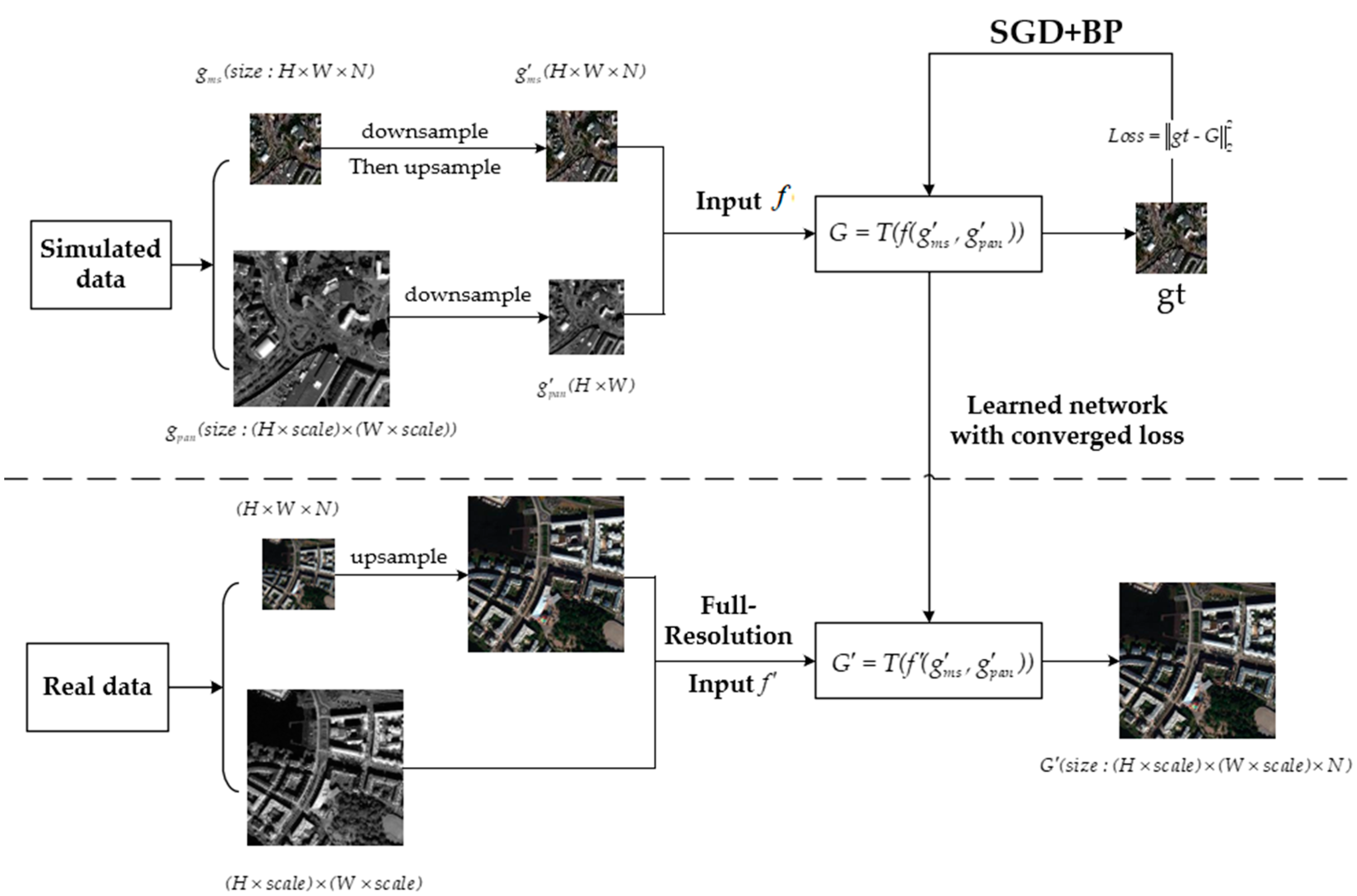
Deep learning technology is a training method with parameters. As shown in Figure 1, we represent the PAN image as and the MS image of N bands as . According to the Wald protocol [46], the MS and PAN images are sampled up and down, respectively, obtaining the degraded images and to form the input data . Through deep network training, the prediction loss between the generated image and the reference image is minimized, and the final data model is obtained. Finally, in the testing phase, the trained data model is used to reconstruct the input real data to generate HRMS images .
3. The Proposed Network
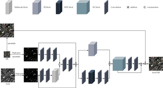
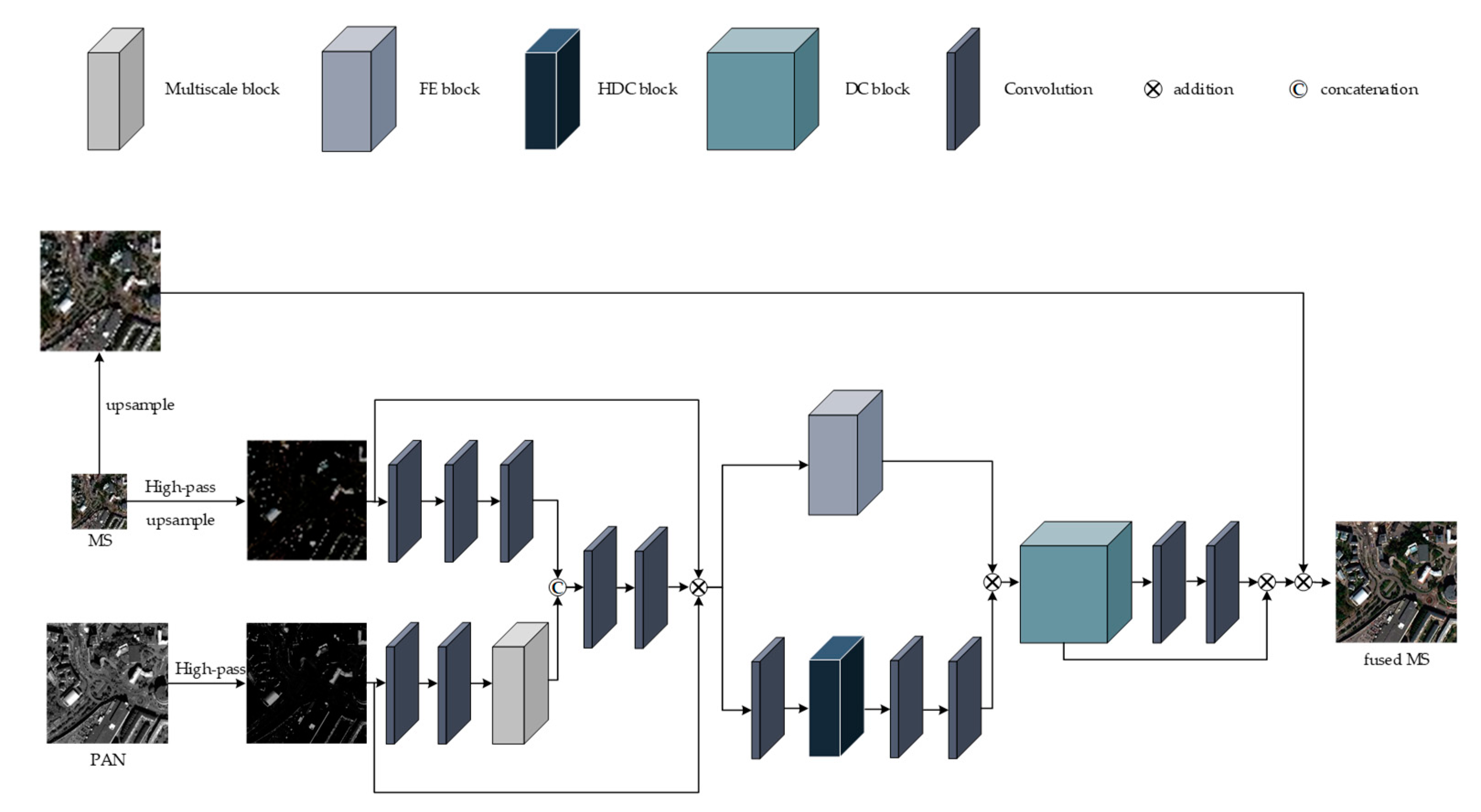
In this chapter, we introduce the proposed MDECNN, as shown in Figure 2. The dual-stream network is used to extract the remote sensing image information contained in the MS image and PAN image, and the fused image is obtained after feature processing and image reconstruction of the fusion network as:
where H denotes the high-pass information, denotes the convolution operation, and denotes the multiscale feature extraction. Finally, we concatenate and to from the fusion features as follows:
where refers to the concatenation operation. Then, the output is obtained through the feature enhancement module and the output is obtained through the dense coding structure as:
where denotes the feature enhancement operation and denotes the dense coded operation. The final prediction is as follows:
We attempt to use deep neural networks to learn the map between the input MS, PAN, and output . We us to represent the reference target and use Loss regularization as the loss function of the training to measure the magnitude of the error between and as follows:
where the function is the matrix norm, especially is the square of Frobenius norm.
To obtain more spatial features, a multiscale feature extraction module was designed to extract the feature information of the PAN image. The feature images extracted from the dual-stream network are superimposed into the trunk network, and the features of different receptive fields of the image are obtained by using the parallel dilated convolution block. After the two-layer convolution, the feature is enhanced by skip connection with the feature enhancement module. Then, a dense coding structure similar to the U-Net structure, is sent for feature fusion and reconstruction. Finally, the fusion image is obtained by enhancing the spectral information of the image by spectral mapping. The weight parameters of the whole network are obtained by learning many nonlinear relationships between simulated data and do not need to be set manually. The details of our proposed network architecture are described below.
3.1. Multiscale Feature Extraction Block
The depth and width of the network have a significant influence on the image fusion results. With a deeper network structure, the network can learn richer feature information and context-dependent mapping. However, with the deepening of the network structure, gradient explosion, gradient disappearance, training difficulties, and other problems often occur. To solve relevant problems, He et al. [47] proposed a residual network structure, the ResNet network structure. By means of skip connection, the training process is optimized, while the network depth is guaranteed. In terms of the width of the network, Szegedy, C. et al. [48] proposed an inception structure, which fully expands the width of the network and enables the network to obtain more characteristic information.
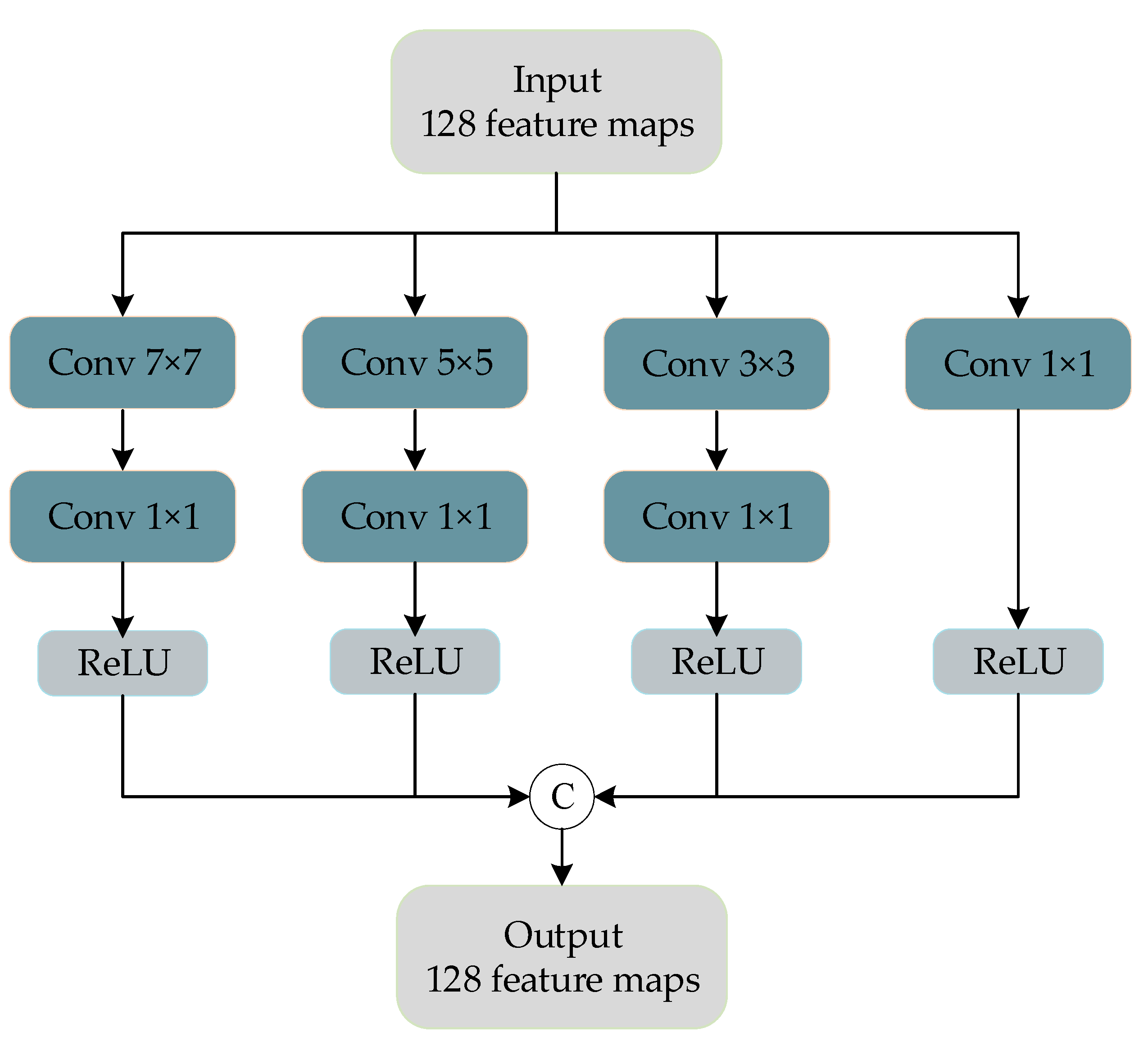
Inspired by GoogLeNet, a multiscale feature extraction block was designed to extract the rich spatial features contained in PAN images. Figure 3 shows the multiscale blocks we designed for feature extraction of PAN images.
The convolution kernels with sizes of , , , and are used for feature extraction of PAN images after two convolution layers. The size of the first three convolution kernels to extract the characteristics of the different sizes of receptive field, using the convolution for dimension reduction of character figure, across the channel characteristics of integration and model simplification, by the multiscale feature extraction piece, we can get rich images in PAN image information.
3.2. Feature Enhancement (FE) Block
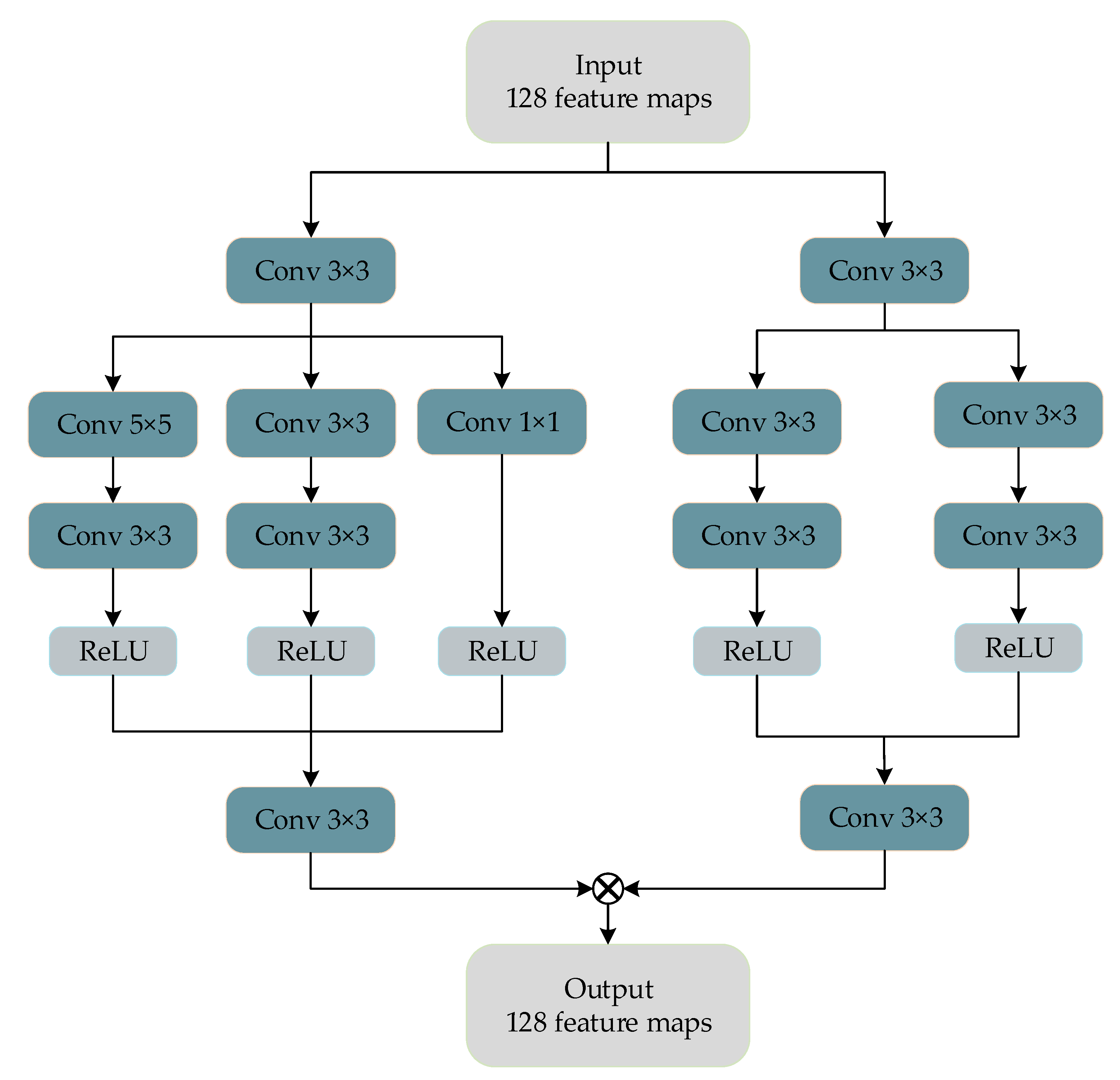
The feature enhancement module is shown in Figure 4.
Remote sensing images contain a large number of buildings, vegetation, mountains, water, and other large-scale objects and contain relatively small-scale target objects such as vehicles, ships, and roads. The traditional convolutional neural network selects the convolution kernel of fixed size, and the receptive field is relatively small, so the context information of the image is not sufficiently learned. To solve this problem, in this paper, the feature enhancement block is proposed. As shown in Figure 4, we select three sensory fields of , , and and do not use an activation function to retain image information when passing through the first convolutional layer. After the first convolutional layer, we use a convolutional layer to enlarge the feature sensory fields and obtain more contextual information.
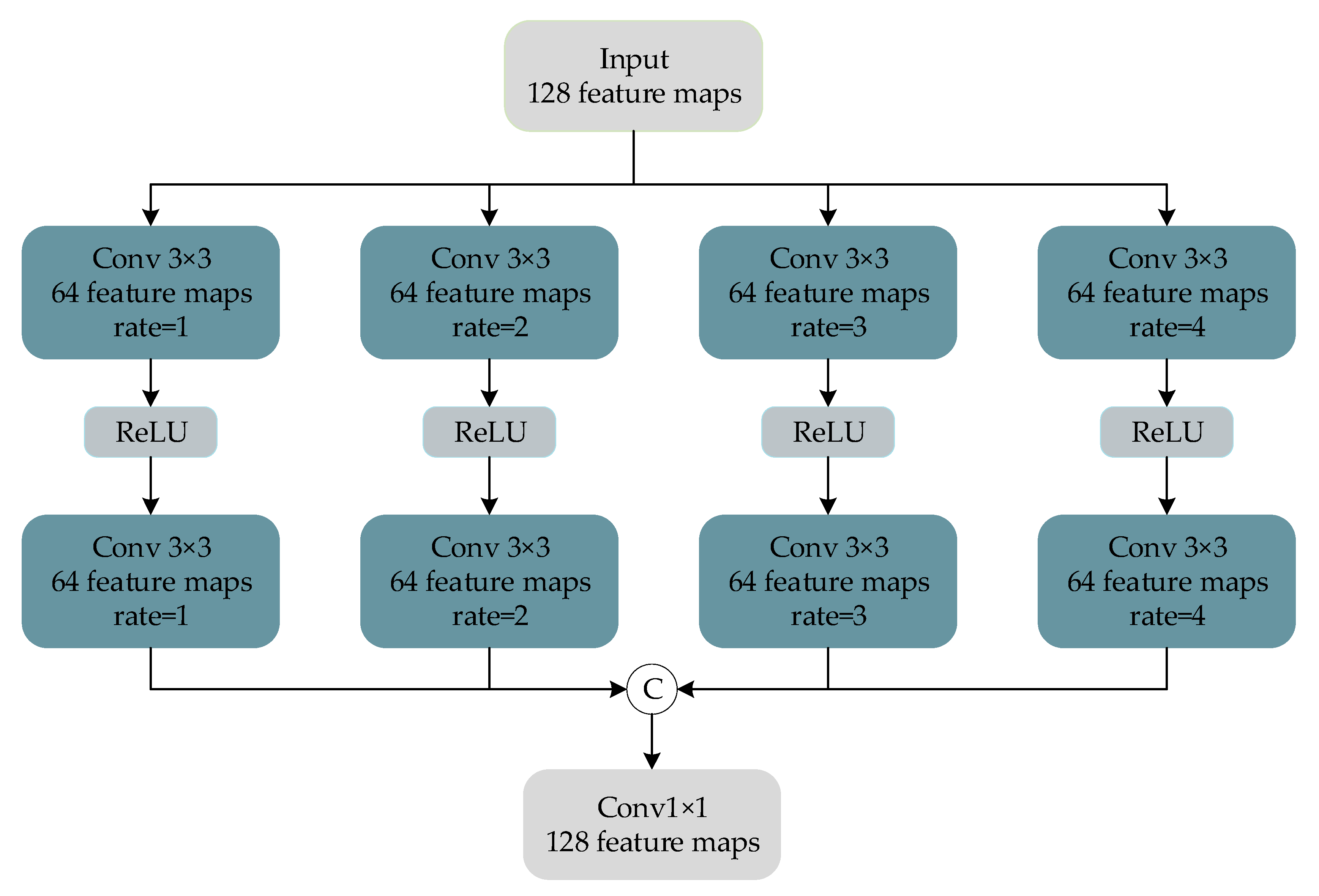
To enhance each feature detail in the remote sensing image, a dilated convolution block, as shown in Figure 5, is designed in the trunk network to extract the multiscale details of the image, and then the features extracted by a skip connection and parallel feature extraction block are stacked to achieve the effect of feature enhancement.
We follow the experimental setting of Fu et al. [30] and set the dilation rate of the dilated convolution block to 1, 2, 3, and 4. The magnitude of the receptive field of the convolution kernel of the dilated convolution is , where d represents the dilation rate, and k represents the size of the convolution kernel. In the parameter setting, the size of the standard convolution kernel and the dilated convolution kernel are both , the activation function is ReLU, and the number of filters is 64. In addition, after the dilated convolution of each layer, a convolutional layer with the same dilation rate is added to further expand the receptive field. Finally, a convolution layer of size is used for dimensionality reduction to reduce computing consumption.
Although the dilated convolution can increase the receptive field of the convolution kernel by expanding the dilation coefficient, it has the problem of “meshing” [49]. In remote sensing images, there are a large number of buildings, vegetation, vehicles, and other objects. These feature-rich objects tend to gather in a large number in the same area, so that there is a strong similarity in the spectrum and spatial structure. Therefore, the use of dilated convolution will lead to the loss of local information from remote sensing images.
To solve this problem, the feature enhancement method, mentioned above, is used to extract multiscale features through parallel feature extraction blocks and to fuse and enhance the features extracted by dilated convolution blocks in the trunk network to improve the robustness of feature extraction in various complex remote sensing images. In addition, through such a feature extraction method, we can extract more perfect spectral information and spatial information and reduce the feature loss in the fusion process.
3.3. Dense Coding (DC) Structure
Considering the abundance of remote sensing image characteristics, a common network structure would not be able to fully extract the deep image characteristics, easily causing information loss in the process of convolution, therefore, we designed a dense coding block to fully image the deep character extraction and avoid common coding in the network layer useful information leakage problems. As shown in Figure 6, in the dense coding network, the feature mapping obtained at each layer is cascaded with the input at the next layer, and the information of the middle layer is retained to the greatest extent by adding channels. At the same time, the feature multiplexing of dense connections does not introduce redundant parameters and does not increase the computing consumption.
There are three advantages to using a block-intensive architecture which are the following: (1) it can hold as much information as possible; (2) this architecture can improve the information flow and gradient flow in the network, making the network easy to train; and (3) intensive contact has a regularized effect, which reduces the over adaptation of tasks [50].
In the decoding stage, to avoid information loss caused by channel plummeting, a U-Net decoding structure similar to the structure of the encoder is used, which is reduced to the number of channels equivalent to the encoder each time to facilitate the full extraction and fusion of features. Its structure is shown in Figure 7.
In the encoding and decoding process, the convolution kernel size is set as and the number of channels is 64, so the reduction of channels at each layer in the decoding process is 64. Through the dense coding structure proposed by us, the deep features of remote sensing images can be fully extracted, and the feature details can be fully recovered in the subsequent image reconstruction process. With the deepening of the network depth, spectral information is often seriously lost. Inspired by PanNet, the spectral mapping method is used to enhance the spectral details of the image in the final image reconstruction part of the network to ensure the spectral quality of the fused image.
3.4. Loss Function
In addition to the network architecture, the loss function is another important factor affecting the fusion image quality. The loss function optimizes the parameters by minimizing the loss between the reconstructed image and the corresponding ground live HR image. Thus, we give a set of training sets , where and represent the PAN image and LRMS image, respectively, and is the corresponding HRMS image. In the existing remote sensing image fusion literature, most of the loss functions used are L2 norm, i.e., root mean square error (MSE). By minimizing the prediction error between the output data and the standard image, the nonlinear mapping relationship between the input image and the output image is learned. The L2 loss function is defined as follows:
where N is the number of small batch samples and i is the ith image. We select the Adam optimizer to carry out back propagation and optimize the allocation of all parameters in the iterative network.
Sharpening the image using L2 losses smooths the image and penalizes larger outliers but is less sensitive to smaller outliers, meaning that the learning process slows significantly as the output approaches the target. To make further improvements, additional small outliers are processed, and image edge information is retained. The L1 norm provides the better effect, with the more pronounced smooth L1 loss defined as follows:
Selecting the L2 norm alone will cause the image to be too smooth and the edge information will be lost. The use of L1 norm alone will lead to insufficient training convergence and serious spectral noise. In view of this problem, we have designed a mixed loss function that uses the combination of L2 loss and smooth L1 loss. The loss of spectral information is constrained by L2 loss and smooth L1 is used as the spatial loss constraint. The mixed loss is defined as follows:
Through experience, the value of is set to 0.3.
4. Experimental Analysis
In this section, we will demonstrate the superiority of the proposed method through experimental results on multiple datasets. By comparing and evaluating the training and test results of the models with different network parameters, the best model is selected for the experiment. Finally, the visual and objective indicators of our best model are compared with several other existing methods to prove the superior performance of the proposed method.
4.1. Dataset and Model Training
To evaluate the performance of our proposed dense coding network based on multiscale perception, we conducted model training and testing on datasets collected by three different satellite sensors, GeoEye-1, Quickbird, and WorldView-3. The band number and spatial resolution of different satellite sensors are shown in Table 1. For the convenience of training, the input images of each dataset are uniformly set as image patch, and the size of each training batch is 4. The train set is used for network training, while the test set is used to evaluate network performance. The spatial resolution of the train set and the test set are shown in Table 2.
The maximum number of training sessions is set to 350,000. For the Adam optimizer, we set the learning rate to 0.001 and the exponential decay factor to 0.9. We set the weight attenuation to . We use the proposed comprehensive loss as a loss function to minimize the prediction error of the model, and the training time of the overall program is approximately 26 h 54 min.
The network is implemented in the TensorFlow deep learning framework and trained on an NVIDIA Tesla V100-SXM2-32GB, and the results are presented with ENVI Classic 5.3.
To facilitate visual observation, the red, green, and blue bands of the multispectral image are used as the imaging bands of the RGB image to form color images. However, in the calculation of objective indicators, other bands of the image will not be ignored.
4.2. Compare Algorithms and Evaluation Methods
For the three experimental datasets, we choose several typical representative methods of pan-sharpening as comparison methods. These include four CS-based methods, i.e., GS [3], PRACS [4], IHS [1], and HPF [29]; two MRA-based methods, i.e., DWT [6] and GLP [8]; one model-based method, i.e., SIRF [13]; and two methods based on the CNN, i.e., PanNet [25] and PSGan [51].
In real application scenes of remote sensing images, HRMS images are often lacking. Therefore, in the comparison algorithm, we use the following two kinds of experiments for comparison: one is the simulation experiment with HRMS images as a reference, and the other is the real experiment without HRMS images. The evaluation criteria of the reference images are as follows: the spectral angle mapper (SAM), the relative average spectral error (RASE), the root mean squared error (RMSE), the universal image quality index (QAVE), the relative dimensionless global error in synthesis (ERGAS), the correlation coefficient (CC), and the structural similarity (SSIM). The other assessments are based on the quality with no reference index (QNR) and the spectral and spatial components ( and ).
4.3. Simulated Experiments
4.3.1. Experiment with WorldView-3 Dataset with Eight Bands
Figure 8 shows a set of fusion results on WorldView-3 satellite data; the data are 8-band data. Figure 8a,b show the HRMS and PAN images with resolution, respectively. Figure 8c–i are seven non-deep learning pan-sharpening methods, and Figure 8j–l are deep learning methods.
Figure 8 shows that seven methods of non-deep learning are accompanied by relatively obvious spectral deviation. Among these methods, DWT and SIRF exhibit obvious spectral distortion, while the edge details of the image are blurred. The IHS fusion image shows partial detail loss in some spectral distortion areas and fuzzy artefacts in road vehicle areas. The HPF, GS, GLP, and PRACS methods show good performance in the overall spatial structure, but they are distorted and blurred in both spectrum and detail. For the fusion method of deep learning, the image texture information performs well, but in terms of spectral information, the fusion method of PSGan shows obvious changes in partial regional spectra, while other differences are not obvious. To further distinguish the image quality, we use the objective evaluation index mentioned before for further comparison. The results are shown in Table 3.
As shown in Table 3, from the perspective of the reference index of WorldView-3 dataset, the pan-sharpening method of deep learning is obviously better than the fusion method of non-deep learning. Among these methods, GLP is superior to other non-deep learning methods in overall effect, and the spectral information of fusion results obtained by HPF and GLP is superior to that obtained by other non-deep learning methods. GLP and PRACS are more complete in preserving spatial information than those of the non-deep learning methods. The results obtained by the PRACS, HPF, and GLP methods showed no significant difference in image quality. In the pan-sharpening method of deep learning, the effectiveness of the network structure directly affects the fusion effect. Therefore, the method proposed in this paper is obviously superior to the existing fusion methods, which proves the effectiveness of the method proposed in this paper.
4.3.2. Experiment with QuickBird Dataset
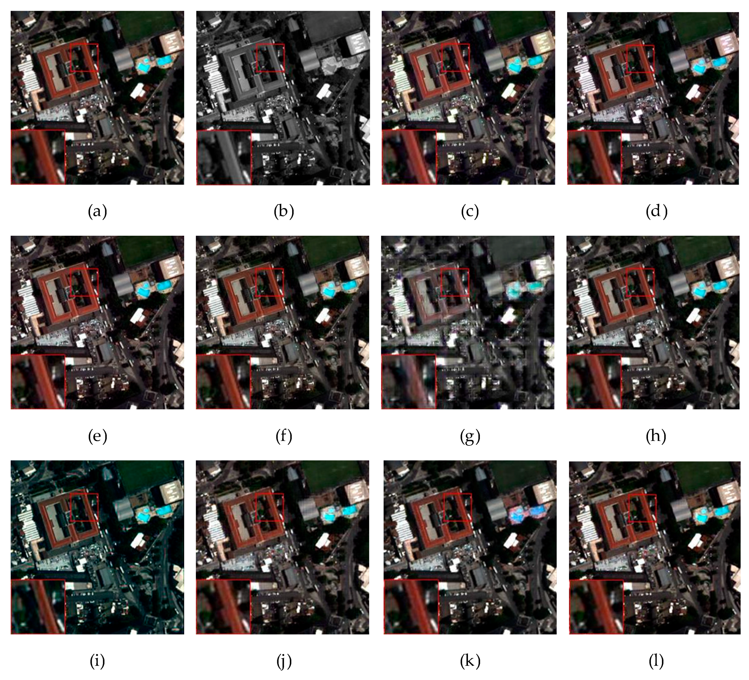
Figure 9 shows a set of fusion results on QuickBird satellite data with a dataset of 4-band images. Figure 9a,b show HRMS and PAN images with resolution, Figure 9c–i represent seven non-deep learning pan-sharpening methods, and Figure 9j–l represent deep learning methods.
In Figure 9, the non-deep learning method obviously has spectral distortion. From Figure 9c–i, the traditional fusion method more or less exhibits the whole spectrum distortion phenomenon. Among the methods, DWT, his, and SIRF present the most severe spectral distortion. GLP and GS present obvious edge blurring in the spectral distortion area, and the PRACS method presents artefacts in the image edge. The deep learning method has good fidelity in both spectral information and spatial information, among which the method proposed by us is the most similar to the original image in both spectral information and spatial information. Table 4 below objectively analyses each method in terms of index values.
As shown in Table 4, the QuickBird experimental assessment results show that the performance of the pan-sharpening method, which is deep learning on the 4-band dataset and is significantly better than the traditional method. In terms of the experimental results of these data, HPF has achieved an overall better performance in traditional methods. Although the HPF method and GLP method are not significantly different in other indicators, the HPF method is obviously superior to the GLP method in maintaining spectral information. PanNet and PSGan have good performance in the deep learning method, but the method proposed in this paper is the best among all the existing methods in terms of all the indicators.
4.3.3. Experiment with GeoEye-1 Dataset
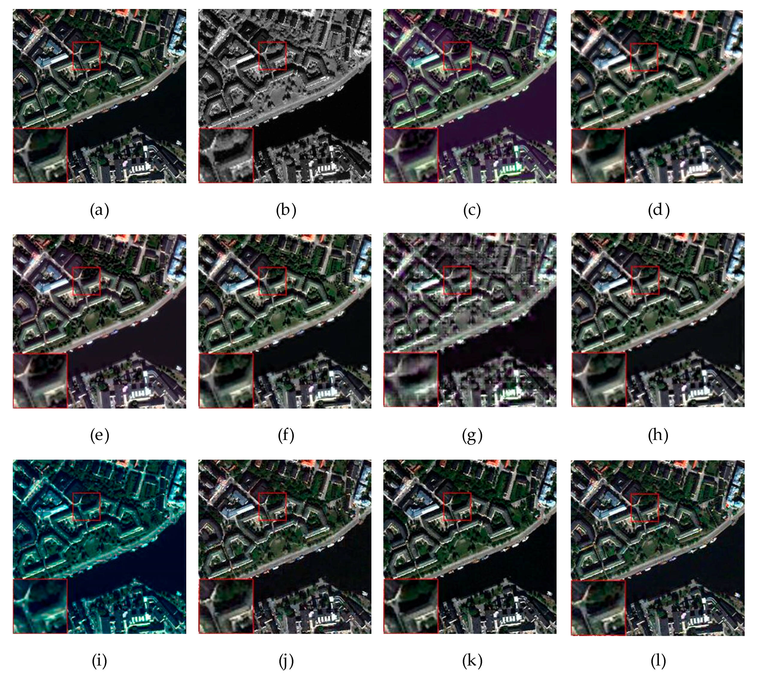
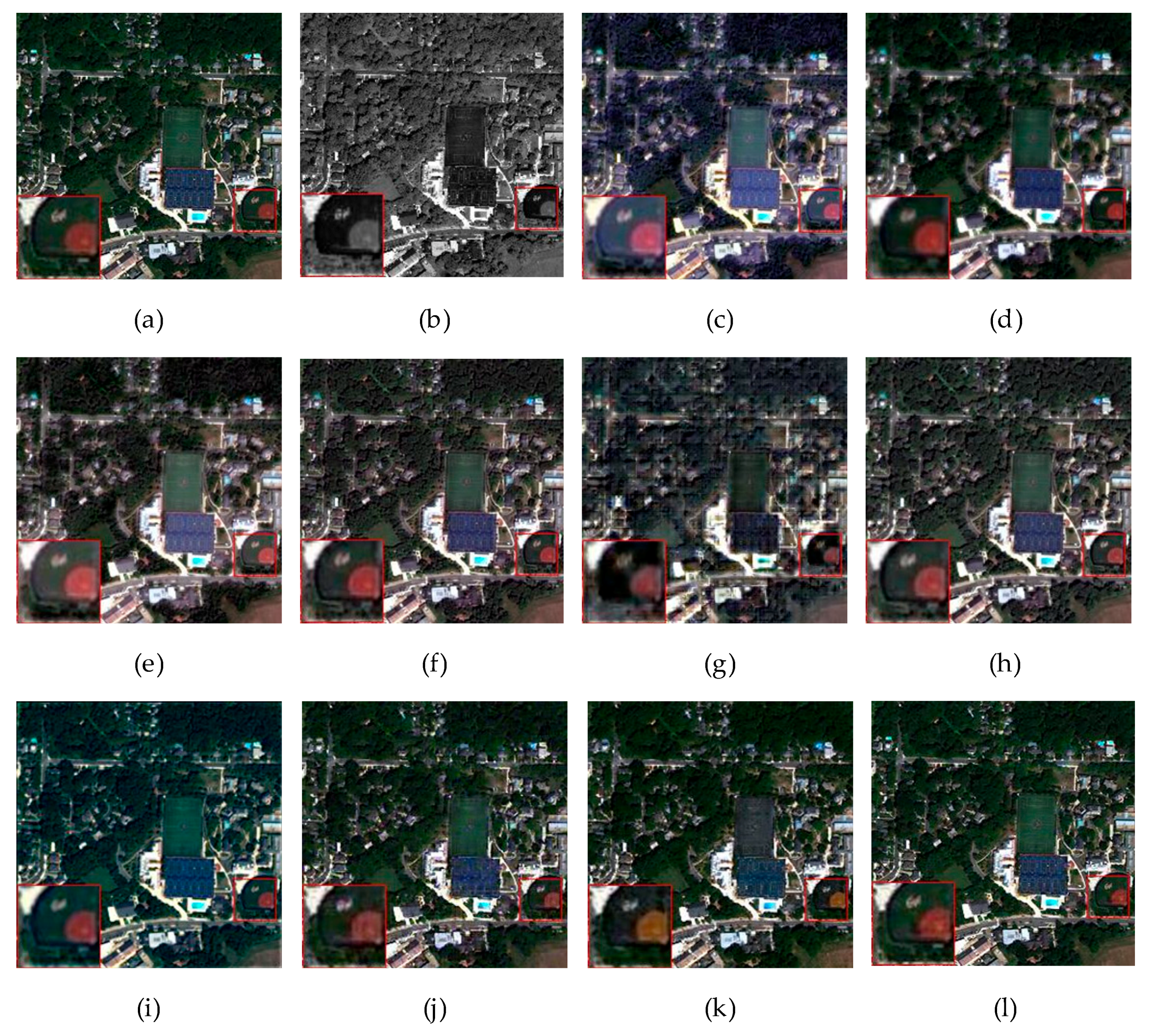
In this section, experiments were performed using a 4-band dataset from GeoEye-1, and the image size is . Figure 10 shows the experimental results of a set of images. Figure 10a,b show HRMS and PAN images, respectively. Figure 10c–i represent seven non-deep learning pan-sharpening methods, while Figure 10j–l represent deep learning methods.
Figure 10 shows that obvious spectral distortion occurs in the DWT, GS, IHS, and SIRF methods, and blurring or loss of edge details occurs in all seven traditional methods. The PRACS method retains good spectral information, but the spatial structure is too smooth, the edge information is severely lost, and there are many artefacts. Compared with GLP and HPF methods, the overall effect is better. In the deep learning method, the PSGan method exhibits spectral distortion in local areas, and the overall effect of deep learning is better than traditional methods. The image from our proposed method is the closest to the original image. The index values shown in Table 5 objectively show the comparison of various methods.
Combined with Table 5, the experimental evaluation indexes of GeoEye-1, QuickBird, and WorldView-3 are roughly the same, which proves the robustness of the network structure proposed by us. Through the above experimental results, the numerical values clearly support the proposed solution, thus, indicating that the proposed solution achieves a significant performance improvement on the same satellite or different satellite, 8-band or 4-band datasets.
4.4. Experiment with GeoEye-1 Real Dataset
Figure 11 shows the pan-sharpening results of the GeoEye-1 image size dataset under real data from unreferenced images. Figure 11a,b show the MS and PAN images, respectively. Figure 11c–l show the DWT, GLP, GS, HPF, IHS, PRACS, SIRF, PanNet, PSGan, and our fusion results of the proposed method.
By observing the fusion images, DWT, IHS, and SIRF all can be found to have obvious spectral distortion, and the edge information of SIRF appears fuzzy. Although the overall spatial structure information is well preserved in the GS and GLP methods, local information is lost. The merged image in the PRACS method is too smooth, resulting in severe loss of edge details. PanNet, PSGan, and our proposed method have the best overall performance, but spectral distortion appears in some regions of PSGan. Table 6 shows that the fusion method proposed by us is the most effective on the real dataset without reference images.
5. Discussion
5.1. Convergence
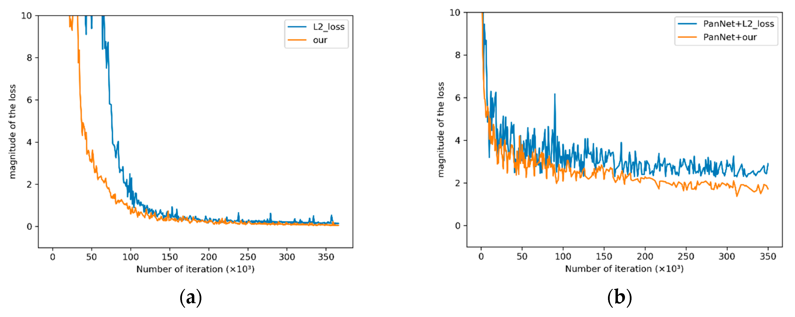
Figure 12 shows the convergence process of L2 loss function and the loss function proposed in this paper on the training set. Table 7 shows the objective evaluation indexes of fused images obtained by different loss functions. The network structure proposed in the paper and the PanNet network structure are used to test the convergence of the loss function. Figure 12a shows the convergence effect of the loss function proposed in this paper of MDECNN, and Figure 12b shows the convergence effect of the loss function proposed in this paper on the network structure of PanNet. The convergence positions of Figure 12a,b indicate that the new loss function training network converges faster and has a better final convergence effect than L2 loss function. At the same time, Table 7 shows that the fused images obtained by the new loss function are more in line with expectations. Meanwhile, by comparing the convergence images in Figure 12a,b, it can be seen that the error fluctuation in Figure 12a is small, indicating that our network structure is more stable and has better convergence effect than that of PanNet. Combined with the results in Figure 12 and Table 7, the proposed solution of the comprehensive loss function is shown to be obviously superior to the general solution of spectral loss L2.
5.2. Ablation Study
We provide ablation learning to explore the impact of each part of our model as follows:
Influence of the multiscale spatial information extraction module This paper focuses on the extraction of rich spatial information and proposes the multiscale spatial information extraction module to independently extract rich spatial information from PAN images. In order to verify the effectiveness of the proposed module and the influence of different receptive field parameters on the fusion results, several convolution blocks with different receptive field sizes are cascaded to form a multiscale feature extraction module. We compare the multiscale block of different scales to test the effect of the multiscale block of different scales. Specifically, we select the best multiscale block by using convolution kernel combinations with different sensory fields, where the convolution kernel size K= {1, 3, 5, 7}. These convolution kernels of different sizes are combined in different ways to obtain the multiscale blocks required by the experiment. To avoid the "meshwork" problem caused by the use of dilated convolution, we use a convolution kernel with different sensory fields to extract feature maps. To make a fair comparison, we adjust the different multiscale blocks so that their parameter numbers are close to each other. The experimental results are shown in Table 8.
The quantitative evaluation results show that the feature information obtained by using a richer receptive field is more expressive. As shown in Table 8, it is obvious that our proposed method is superior to other receptive field sets under different orders of magnitude. Therefore, to balance the performance and computing speed, we use four multiscale sensing modules with different sensing fields, namely, 1, 3, 5, and 7.
Influence of the feature enhancement module Influenced by the inception module, we propose the structure of the feature enhancement module. To validate its impact, we remove the feature enhancement module and add more modules to validate its impact. We experiment on the trunk network without the feature enhancement module and the double-branch network with two feature enhancement modules cascaded. Fusion results are obtained and compared. The quantitative results are shown in Table 9.
As seen from the quantitative evaluation results, using a feature enhancement module to broaden the width of the network can enable the network to extract richer feature information and learn more mapping relationships in line with expectations. Failure to use feature enhancement modules led to insufficient learning ability of the model for multiscale features, inadequate learning of details, and decreased ability of image reconstruction. However, using too many feature enhancement modules would lead to convergence difficulty or feature explosion, increasing the computing consumption and also affecting the network convergence effect. Therefore, based on the results of the experiment, we choose to use one feature enhancement module to deal with features for our network.
Setting of encoding network parameters We also test the influence of encoding network depth. Specifically, we fix the other module parameters, and then we set the encoding network depth to L= {3, 6, 12, 14, 16} for verification. The model is trained by using the coding networks of 3, 6, 12, 14, and 16 dense-coded layers and the decoding networks of corresponding layers to obtain the corresponding fusion images. Meanwhile, objective evaluation indexes are used to observe the visual statistics on the results, and the quantitative results are shown in Figure 13.
The objective evaluation index shows that increasing the depth of the dense coding network can improve the performance of the network, and the performance of the network can be significantly improved when the depth of the coding network increases. The reason lies in the increase in network depth and width, which enhances the ability of network to extract and reconstruct high latitude features. However, when the network depth is greater than 16 layers and the network is too deep and wide, the redundancy of feature extraction is increased, and the loss of features is also caused, resulting in the convergence difficulty of the network. Figure 13 shows that the depth of the coding network affects the performance of the network. After testing, the depth of the dense coding network was finally set to 14.
6. Conclusions
In this paper, we propose a deep learning-based method to solve the pan-sharpening problem by combining convolutional neural network technology and domain-specific knowledge. On the basis of the existing pan-sharpening solutions, multiscale feature blocks are designed to process PAN images separately to extract richer and more complete spatial information, feature enhancement blocks and dense coding networks are used to learn more accurate mapping relationships, and comprehensive loss functions are designed to constrain image loss. Better fusion images can be obtained with full consideration of different spectral and spatial characteristics. In remote sensing images, regional spatial structure, land cover and development characteristics are diverse. Because the method proposed in this paper is more sensitive to multiscale features in theory, MDECNN can achieve better results in different types of remote sensing images in areas with different sizes of seeding sites, diverse structures in densely built areas, and different urban greening proportions. It is significant for remote sensing image fusion of complex image information. At the same time, in some remote sensing images with relatively single image features, the improvement of fusion effect of the proposed method is relatively limited, which reflects the limitations of multiscale feature image fusion. The experimental results of three kinds of satellite datasets show that the proposed method can perform better than the existing methods in the pan-sharpening of a wide range of satellite data, which proves the potential value of our network for different tasks. Next, we will take the loss function with the constraint of objective indexes as the starting point to further improve the network performance on the premise of ensuring the spectrum and space quality.
Author Contributions
Data curation, W.L.; formal analysis, W.L.; methodology, W.L. and X.L.; validation, X.L.; visualization, M.D.; writing—original draft, X.L.; writing—review and editing, M.D. All authors have read and agreed to the published version of the manuscript.
Funding
This research was funded by the National Natural Science Foundation of China ((no. 61972060, U171321, and 62027827), the National Key Research and Development Program of China (no. 2019YFE0110800), the Natural Science Foundation of Chongqing (cstc2020jcyj-zdxmX0025 and cstc2019cxcyljrc-td0270), and the Chongqing Graduate Student Research and Innovation Project (no. CYS20255).
Data Availability Statement
Data sharing is not applicable to this article.
Acknowledgments
The authors would like to thank all the reviewers for their valuable contributions to our work.
Conflicts of Interest
The authors declare no conflict of interest.
References
- Tu, T.-M.; Su, S.-C.; Shyu, H.-C.; Huang, P.S. A new look at IHS-like image fusion methods. Inf. Fusion 2001, 2, 177–186. [Google Scholar] [CrossRef]
- Kwarteng, P.; Chavez, A. Extracting spectral contrast in Landsat Thematic Mapper image data using selective principal component analysis. Photogramm. Eng. Remote Sens. 1989, 55, 339–348. [Google Scholar]
- Laben, C.A.; Brower, B.V. Process for Enhancing the Spatial Resolution of Multispectral Imagery Using Pan-Sharpening. U.S. Patent 6,011,875, 4 January 2000. [Google Scholar]
- Choi, J.; Yu, K.; Kim, Y. A new adaptive component-substitution-based satellite image fusion by using partial replacement. IEEE Trans. Geosci. Remote Sens. 2011, 49, 295–309. [Google Scholar] [CrossRef]
- Restaino, R.; Mura, M.D.; Vivone, G.; Chanussot, J. Context-Adaptive Pansharpening Based on Image Segmentation. IEEE Trans. Geosci. Remote Sens. 2017, 55, 753–766. [Google Scholar] [CrossRef] [Green Version]
- Zhou, J.; Civco, D.L.; Silander, J.A. A wavelet transform method to merge Landsat TM and SPOT panchromatic data. Int. J. Remote Sens. 1998, 19, 743–757. [Google Scholar] [CrossRef]
- Aiazzi, B.; Alparone, L.; Baronti, S.; Garzelli, A. Context-driven fusion of high spatial and spectral resolution images based on oversampled multiresolution analysis. IEEE Trans. Geosci. Remote Sens. 2002, 40, 2300–2312. [Google Scholar] [CrossRef]
- Otazu, X.; Gonzalez-Audicana, M.; Fors, O.; Nunez, J. Introduction of sensor spectral response into image fusion methods. Application to wavelet-based methods. IEEE Trans. Geosci. Remote Sens. 2005, 43, 2376–2385. [Google Scholar] [CrossRef] [Green Version]
- Nunez, J.; Otazu, X.; Fors, O.; Prades, A.; Pala, V.; Arbiol, R. Multiresolution-based image fusion with additive wavelet decomposition. IEEE Trans. Geosci. Remote Sens. 1999, 37, 1204–1211. [Google Scholar] [CrossRef] [Green Version]
- Khan, M.; Chanussot, J.; Condat, L.; Montanvert, A. Indusion: Fusion of Multispectral and Panchromatic Images Using the Induction Scaling Technique. IEEE Geosci. Remote Sens. Lett. 2008, 5, 98–102. [Google Scholar] [CrossRef] [Green Version]
- Nencini, F.; Garzelli, A.; Baronti, S. Remote sensing image fusion using the curvelet transform. Inf. Fusion 2007, 8, 143–156. [Google Scholar] [CrossRef]
- Shah, V.P.; Younan, N.H.; King, R.L. An Efficient Pan-Sharpening Method via a Combined Adaptive PCA Approach and Contourlets. IEEE Trans. Geosci. Remote Sens. 2008, 46, 1323–1335. [Google Scholar] [CrossRef]
- Burger, H.C.; Schuler, C.J.; Harmeling, S. Image denoising: Can plain neural networks compete with BM3D? In Proceedings of the IEEE Conference on Computer Vision and Pattern Recognition, Providence, RI, USA, 16–21 June 2012; pp. 2392–2399. [Google Scholar]
- Xu, M.; Chen, H. An image fusion approach based on Markov random fields. IEEE Trans. Geosci. Remote Sens. 2011, 49, 5116–5127. [Google Scholar]
- Ballester, C.; Caselles, V.; Igual, L.; Verdera, J.; Rougé, B. A variational model for P+ XS image fusion. Int. J. Comput. 2006, 69, 43–58. [Google Scholar] [CrossRef]
- Palsson, F.; Ulfarsson, M.O.; Sveinsson, J.R. Model-Based Reduced-Rank Pansharpening. IEEE Geosci. Remote. Sens. Lett. 2019, 17, 656–660. [Google Scholar] [CrossRef]
- Zhang, L.; Shen, H.; Gong, W.; Zhang, H. Adjustable model-based fusion method for multispectral and panchromatic images. IEEE Trans. Syst. Man Cybern. Part B 2012, 42, 1693–1704. [Google Scholar] [CrossRef] [PubMed]
- Li, S.; Yang, B. A new pan-sharpening method using a compressed sensing technique. IEEE Trans. Geosci. Remote Sens. 2010, 49, 738–746. [Google Scholar] [CrossRef]
- Ghahremani, M.; Ghassemian, H. A compressed-sensing-based pan-sharpening method for spectral distortion reduction. IEEE Trans. Geosci. Remote Sens. 2016, 54, 2194–2206. [Google Scholar] [CrossRef]
- Li, S.; Yin, H.; Fang, L. Remote sensing image fusion via sparse representations over learned dictionaries. IEEE Trans. Geosci. Remote Sens. 2013, 51, 4779–4789. [Google Scholar] [CrossRef]
- Shahdoosti, H.R.; Mehrabi, A. Multimodal image fusion using sparse representation classification in tetrolet domain. Digit. Signal Process. 2018, 79, 9–22. [Google Scholar] [CrossRef]
- Dong, C.; Loy, C.C.; He, K.; Tang, X. Learning a deep convolutional network for image super-resolution. In Proceedings of the European Conference on Computer Vision, Zurich, Switzerland, 6–12 September 2014; pp. 184–199. [Google Scholar]
- Masi, G.; Cozzolino, D.; Verdoliva, L.; Scarpa, G. Pansharpening by convolutional neural networks. Remote Sens. 2016, 8, 594. [Google Scholar] [CrossRef] [Green Version]
- Wei, Y.; Yuan, Q.; Shen, H.; Zhang, L. Boosting the accuracy of multispectral image pansharpening by learning a deep residual network. IEEE Geosci. Remote Sens. Lett. 2017, 14, 1795–1799. [Google Scholar] [CrossRef] [Green Version]
- Yang, J.; Fu, X.; Hu, Y.; Huang, Y.; Ding, X.; Paisley, J. PanNet: A deep network architecture for pan-sharpening. In Proceedings of the IEEE International Conference on Computer Vision, Venice, Italy, 22–29 October 2017; pp. 5449–5457. [Google Scholar]
- Rahmani, S.; Strait, M.; Merkurjev, D.; Moeller, M.; Wittman, T. An adaptive IHS pan-sharpening method. IEEE Geosci. Remote. Sens. Lett. 2010, 7, 746–750. [Google Scholar] [CrossRef] [Green Version]
- Shi, Y.; Wanyu, Z.; Wei, L. Pansharpening of Multispectral Images based on Cycle-spinning Quincunx Lifting Transform. In Proceedings of the IEEE International Conference on Signal, Information and Data Processing, Chongqing, China, 11–13 December 2019; pp. 1–5. [Google Scholar]
- Giraud, L.; Langou, J.; Rozloznik, M. The loss of orthogonality in the Gram-Schmidt orthogonalization process. Comput. Math. Appl. 2005, 50, 1069–1075. [Google Scholar] [CrossRef] [Green Version]
- Witharana, C.; Civco, D.L.; Meyer, T.H. Evaluation of pansharpening algorithms in support of earth observation based rapid-mapping workflows. Appl. Geogr. 2013, 37, 63–87. [Google Scholar] [CrossRef]
- Fu, X.; Wang, W.; Huang, Y.; Ding, X.; Paisley, J. Deep Multiscale Detail Networks for Multiband Spectral Image Sharpening. IEEE Trans. Neural Netw. Learn. Syst. 2020, 99, 1–15. [Google Scholar] [CrossRef]
- Zhong, J.; Yang, B.; Huang, G.; Zhong, F.; Chen, Z. Remote sensing image fusion with convolutional neural network. Sens. Imaging 2016, 17, 1–16. [Google Scholar] [CrossRef]
- Yuan, Q.; Wei, Y.; Meng, X.; Shen, H.; Zhang, L. A multiscale and multidepth convolutional neural network for remote sensing imagery pan-sharpening. IEEE J. Sel. Top. Appl. Earth Obs. Remote Sens. 2018, 11, 978–989. [Google Scholar] [CrossRef] [Green Version]
- Kim, J.; Lee, J.K. Accurate image super-resolution using very deep convolutional networks. In Proceedings of the IEEE Conference on Computer Vision and Pattern Recognition, Las Vegas, NV, USA, 27–30 June 2016; pp. 1646–1654. [Google Scholar]
- Ledig, C. Photo-realistic single image super-resolution using a generative adversarial network. In Proceedings of the IEEE Conference on Computer Vision and Pattern Recognition, Honolulu, HI, USA, 21–26 July 2017; pp. 4681–4690. [Google Scholar]
- Huang, G.; Liu, Z.; Van Der Maaten, L.; Weinberger, K.Q. Densely connected convolutional networks. In Proceedings of the IEEE Conference on Computer Vision and Pattern Recognition, Honolulu, HI, USA, 21–26 July 2017; pp. 4700–4708. [Google Scholar]
- Kim, J.; Lee, J.K.; Lee, K.M. Deeply-recursive convolutional network for image super-resolution. In Proceedings of the IEEE Conference on Computer Vision and Pattern Recognition, Las Vegas, NV, USA, 27–30 June 2016; pp. 1637–1645. [Google Scholar]
- Tai, Y.; Yang, J.; Liu, X. Image super-resolution via deep recursive residual network. In Proceedings of the IEEE Conference on Computer Vision and Pattern Recognition, Honolulu, HI, USA, 21–26 July 2017; pp. 3147–3155. [Google Scholar]
- Dong, C.; Loy, C.; Tang, X. Accelerating the super-resolution convolutional neural network. In Proceedings of the European Conference on Computer Vision; Springer: Cham, Switzerland, 2016; pp. 391–407. [Google Scholar]
- Jiang, C.; Zhang, H.; Shen, H.; Zhang, L. Two-step sparse coding for the pan-sharpening of remote sensing images. IEEE J. Sel. Top. Appl. Earth Obs. Remote Sens. 2013, 7, 1792–1805. [Google Scholar] [CrossRef]
- Huang, W.; Xiao, L.; Wei, Z.; Liu, H.; Tang, S. A new pan-sharpening method with deep neural networks. IEEE Geosci. Remote Sens. Lett. 2015, 12, 1037–1041. [Google Scholar] [CrossRef]
- Rao, Y.; He, L.; Zhu, J. A residual convolutional neural network for pan-shaprening. In Proceedings of the International Workshop on Remote Sensing with Intelligent Processing (RSIP), Shanghai, China, 19–21 May 2017; pp. 1–4. [Google Scholar]
- Scarpa, G.; Vitale, S.; Cozzolino, D. Target-adaptive CNN-based pansharpening. IEEE Trans. Geosci. Remote Sens. 2018, 56, 5443–5457. [Google Scholar] [CrossRef] [Green Version]
- Azarang, A.; Ghassemian, H. A new pansharpening method using multi resolution analysis framework and deep neural networks. In Proceedings of the 3rd International Conference on Pattern Recognition and Image Analysis (IPRIA), Shahrekord, Iran, 19–20 April 2017; pp. 1–6. [Google Scholar]
- Vitale, S. A CNN-based Pansharpening Method with Perceptual Loss. In Proceedings of the IEEE International Geoscience and Remote Sensing Symposium, Yokohama, Japan, 28 July–2 August 2019; pp. 3105–3108. [Google Scholar]
- Li, Z.; Cheng, C. A CNN-Based Pan-Sharpening Method for Integrating Panchromatic and Multispectral Images Using Landsat 8. Remote Sens. 2019, 11, 2606. [Google Scholar] [CrossRef] [Green Version]
- Wald, L.; Ranchin, T.; Marc, M. Fusion of satellite images of different spatial resolutions: Assessing the quality of resulting images. Photogramm. Eng. Remote Sens. 1997, 63, 691–699. [Google Scholar]
- He, K.; Zhang, X.; Ren, S.; Sun, J. Deep residual learning for image recognition. In Proceedings of the IEEE Conference on Computer Vision and Pattern Recognition, Las Vegas, NV, USA, 27–30 June 2016; pp. 770–778. [Google Scholar]
- Szegedy, C.; Vanhoucke, V.; Ioffe, S.; Shlens, J.; Wojna, Z. Rethinking the inception architecture for computer vision. In Proceedings of the IEEE Conference on Computer Vision and Pattern Recognition, Las Vegas, NV, USA, 27–30 June 2016; pp. 2818–2826. [Google Scholar]
- Yu, F.; Koltun, V.; Funkhouser, T. Dilated residual networks. In Proceedings of the IEEE Conference on Computer Vision and Pattern Recognition, Honolulu, HI, USA, 21–26 July 2017; pp. 472–480. [Google Scholar]
- Ding, G.; Guo, Y.; Chen, K.; Chu, C.; Han, J.; Dai, Q. DECODE: Deep confidence network for robust image classification. IEEE Trans. Image Process. 2019, 28, 3752–3765. [Google Scholar] [CrossRef] [PubMed] [Green Version]
- Liu, X.; Wang, Y.; Liu, Q. PSGAN: A generative adversarial network for remote sensing image pan-sharpening. In Proceedings of the IEEE International Conference on Image Processing, Athens, Greece, 7–10 October 2018; pp. 873–877. [Google Scholar]
Figure 1.
Workflow of the proposed convolutional neural network (CNN)-based pan-sharpening.

Figure 2.
The detailed architecture of the proposed multiscale perception dense coding convolutional neural network (MDECNN).
Figure 2.
The detailed architecture of the proposed multiscale perception dense coding convolutional neural network (MDECNN).

Figure 3.
Multiscale feature extraction block structure.

Figure 4.
Feature enhancement module structure.

Figure 5.
Hybrid dilated convolution (HDC) module.

Figure 6.
Dense coding structure.

Figure 7.
Decoding structure.

Figure 8.
Results of the WorldView-3 dataset with four bands and 256 × 256 size. (a) Reference image; (b) panchromatic (PAN) image; (c) intensity-hue saturation (IHS); (d) partial substitution (PRACS); (e) Gram–Schmidt (GS); (f) HPF; (g) multi-resolution analysis-based method DWT; (h) multi-resolution analysis-based method GLP; (i) model-based method SIRF; (j) CNN-based method PanNet; (k) CNN-based method PSGan; (l) MDECNN.

Figure 9.
Results of the QuickBird dataset with four bands and 256 × 256 size. (a) Reference image; (b) PAN image; (c) IHS; (d) PRACS; (e) GS; (f) HPF; (g) DWT; (h) GLP; (i) SIRF; (j) PanNet; (k) PSGan; (l) MDECNN.
Figure 9.
Results of the QuickBird dataset with four bands and 256 × 256 size. (a) Reference image; (b) PAN image; (c) IHS; (d) PRACS; (e) GS; (f) HPF; (g) DWT; (h) GLP; (i) SIRF; (j) PanNet; (k) PSGan; (l) MDECNN.

Figure 10.
Results of the GeoEye-1 dataset with eight bands and 256 × 256 size. (a) Reference image; (b) PAN image; (c) HIS; (d) PRACS; (e) GS; (f) HPF; (g) DWT; (h) GLP; (i) SIRF; (j) PanNet; (k) PSGan; (l) MDECNN.
Figure 10.
Results of the GeoEye-1 dataset with eight bands and 256 × 256 size. (a) Reference image; (b) PAN image; (c) HIS; (d) PRACS; (e) GS; (f) HPF; (g) DWT; (h) GLP; (i) SIRF; (j) PanNet; (k) PSGan; (l) MDECNN.

Figure 11.
Results of the GeoEye-1 real dataset with four bands and 256 × 256 size. (a) Reference image; (b) PAN image; (c) IHS; (d) PRACS; (e) GS; (f) HPF; (g) DWT; (h) GLP; (i) SIRF; (j) PanNet; (k) PSGan; (l) MDECNN.
Figure 11.
Results of the GeoEye-1 real dataset with four bands and 256 × 256 size. (a) Reference image; (b) PAN image; (c) IHS; (d) PRACS; (e) GS; (f) HPF; (g) DWT; (h) GLP; (i) SIRF; (j) PanNet; (k) PSGan; (l) MDECNN.

Figure 12.
Convergence images of different loss functions. (a) The convergence of different loss functions corresponding to the network structure proposed in this paper; (b)The convergence of different loss functions corresponding to PanNet.
Figure 12.
Convergence images of different loss functions. (a) The convergence of different loss functions corresponding to the network structure proposed in this paper; (b)The convergence of different loss functions corresponding to PanNet.

Figure 13.
Figure of quantitative assessment results of different coding network parameters.


Table 1.
The spatial resolution of datasets from different satellites.
| Sensors | Bands | PAN (GSD at Nadir) | MS (GSD at Nadir) |
|---|---|---|---|
| GeoEye-1 | 4 | 0.41 m | 1.65 m |
| Quickbird | 4 | 0.61 m | 2.44 m |
| WorldView-3 | 8 | 0.31 m | 1.24 m |
Table 2.
The spatial resolution of datasets from different satellites.
| Dataset | Train Set | Test Set |
|---|---|---|
| GeoEye-1 | 750 | 200 |
| Quickbird | 750 | 200 |
| WorldView-3 | 1000 | 300 |
Table 3.
Quantitative assessment of the WorldView-3 dataset is shown in Figure 8. The best performance is shown in bold.
Table 3.
Quantitative assessment of the WorldView-3 dataset is shown in Figure 8. The best performance is shown in bold.
| Method | SAM | RASE | RMSE | Q_AVE | ERGAS | CC | SSIM |
|---|---|---|---|---|---|---|---|
| IHS | 3.5833 | 17.6374 | 0.0303 | 0.8141 | 4.4781 | 0.9640 | 0.7943 |
| PRACS | 3.6699 | 15.9310 | 0.0274 | 0.8334 | 3.9593 | 0.9681 | 0.8117 |
| GS | 3.3445 | 17.4713 | 0.0301 | 0.8210 | 4.4143 | 0.9648 | 0.8020 |
| HPF | 3.2204 | 16.0554 | 0.0276 | 0.8175 | 4.0414 | 0.9678 | 0.7888 |
| DWT | 7.9628 | 26.8781 | 0.0507 | 0.6631 | 6.8043 | 0.9069 | 0.6248 |
| GLP | 3.3376 | 16.0915 | 0.0277 | 0.8280 | 4.0460 | 0.9702 | 0.8061 |
| SIRF | 4.8736 | 16.0130 | 0.0277 | 0.8066 | 4.2910 | 0.9690 | 0.7985 |
| PanNet | 3.2644 | 12.6437 | 0.0218 | 0.8519 | 3.1523 | 0.9800 | 0.8309 |
| PSGan | 3.0051 | 12.3693 | 0.0210 | 0.8863 | 3.0607 | 0.9816 | 0.8788 |
| MDECNN | 2.0007 | 8.1989 | 0.0141 | 0.9306 | 2.0609 | 0.9917 | 0.9231 |
Table 4.
Quantitative assessment of the QuickBird dataset shown in Figure 9. The best performance is shown in bold.
Table 4.
Quantitative assessment of the QuickBird dataset shown in Figure 9. The best performance is shown in bold.
| Method | SAM | RASE | RMSE | Q_AVE | ERGAS | CC | SSIM |
|---|---|---|---|---|---|---|---|
| IHS | 7.5079 | 29.8941 | 0.0390 | 0.6634 | 7.7151 | 0.9299 | 0.7206 |
| PRACS | 6.5212 | 30.1369 | 0.0393 | 0.6341 | 8.2774 | 0.9211 | 0.6860 |
| GS | 7.3094 | 29.0126 | 0.0378 | 0.6647 | 7.7323 | 0.9363 | 0.7220 |
| HPF | 6.4087 | 26.5668 | 0.0346 | 0.6906 | 7.0718 | 0.9375 | 0.7470 |
| DWT | 13.8999 | 42.2315 | 0.0553 | 0.5275 | 10.7812 | 0.8322 | 0.5634 |
| GLP | 6.8212 | 26.8050 | 0.0350 | 0.6952 | 7.1060 | 0.9350 | 0.7518 |
| SIRF | 11.5283 | 35.9064 | 0.0483 | 0.5683 | 10.5544 | 0.8746 | 0.6212 |
| PanNet | 4.8238 | 18.7275 | 0.0246 | 0.7329 | 5.0167 | 0.9687 | 0.7766 |
| PSGan | 4.3774 | 20.0302 | 0.0258 | 0.7405 | 5.3411 | 0.9654 | 0.7981 |
| MDECNN | 3.3550 | 13.1669 | 0.0171 | 0.8328 | 3.5883 | 0.9849 | 0.8640 |
Table 5.
Quantitative assessment of the GeoEye-1 dataset shown in Figure 10. The best performance is shown in bold.
Table 5.
Quantitative assessment of the GeoEye-1 dataset shown in Figure 10. The best performance is shown in bold.
| Method | SAM | RASE | RMSE | Q_AVE | ERGAS | CC | SSIM |
|---|---|---|---|---|---|---|---|
| IHS | 7.5153 | 29.6974 | 0.0505 | 0.6557 | 6.1735 | 0.9291 | 0.6355 |
| PRACS | 7.0326 | 30.8486 | 0.0524 | 0.6366 | 6.1633 | 0.9219 | 0.6072 |
| GS | 7.1742 | 28.9810 | 0.0492 | 0.6699 | 5.9869 | 0.9334 | 0.6550 |
| HPF | 7.0388 | 25.4033 | 0.0432 | 0.7418 | 5.0361 | 0.9475 | 0.7185 |
| DWT | 13.4489 | 50.4446 | 0.0801 | 0.4996 | 9.9815 | 0.8645 | 0.4790 |
| GLP | 7.1957 | 25.6215 | 0.0436 | 0.7397 | 5.0448 | 0.9462 | 0.7185 |
| SIRF | 6.9346 | 26.7501 | 0.0455 | 0.6903 | 5.5004 | 0.9413 | 0.6703 |
| PanNet | 5.1240 | 20.2831 | 0.0344 | 0.7430 | 4.5522 | 0.9668 | 0.7308 |
| PSGan | 6.3814 | 26.4536 | 0.0449 | 0.7103 | 5.4148 | 0.9433 | 0.6972 |
| MDECNN | 2.1406 | 11.4061 | 0.0193 | 0.9188 | 2.5704 | 0.9897 | 0.9122 |
Table 6.
Quantitative assessment of the GeoEye-1 real dataset shown in Figure 11. The best performance is shown in bold.
Table 6.
Quantitative assessment of the GeoEye-1 real dataset shown in Figure 11. The best performance is shown in bold.
| Method | QNR | ||
|---|---|---|---|
| IHS | 0.8753 | 0.0531 | 0.0756 |
| PRACS | 0.9013 | 0.0183 | 0.0818 |
| GS | 0.8636 | 0.0477 | 0.0931 |
| HPF | 0.7974 | 0.0848 | 0.1287 |
| DWT | 0.5506 | 0.2805 | 0.2347 |
| GLP | 0.8026 | 0.1073 | 0.1010 |
| SIRF | 0.9100 | 0.0660 | 0.0257 |
| PanNet | 0.9052 | 0.0235 | 0.0731 |
| PSGan | 0.8887 | 0.0245 | 0.0888 |
| MDECNN | 0.9190 | 0.0166 | 0.0655 |
Table 7.
Quantitative evaluation results of different loss functions. The best performance is shown in bold.
Table 7.
Quantitative evaluation results of different loss functions. The best performance is shown in bold.
| Setting | SAM | RASE | RMSE | Q_AVE | ERGAS | CC | SSIM |
|---|---|---|---|---|---|---|---|
| PanNet+L2 | 5.4322 | 21.3489 | 0.0365 | 0.7320 | 4.7609 | 0.9627 | 0.7183 |
| PanNet+our | 5.3997 | 21.0970 | 0.0359 | 0.7354 | 4.7374 | 0.9641 | 0.7229 |
| Proposed+L2 | 3.2503 | 13.4427 | 0.0229 | 0.8570 | 3.1788 | 0.9855 | 0.8528 |
| Proposed | 2.7442 | 12.3498 | 0.0208 | 0.8886 | 2.7651 | 0.9881 | 0.8827 |
Table 8.
Quantitative assessment results of multiscale feature extraction module. The best performance is shown in bold.
Table 8.
Quantitative assessment results of multiscale feature extraction module. The best performance is shown in bold.
| DF | SAM | RASE | RMSE | Q_AVE | ERGAS | CC | SSIM |
|---|---|---|---|---|---|---|---|
| K = {1, 3, 5, 5} | 3.1916 | 12.5804 | 0.0214 | 0.8566 | 3.0728 | 0.9873 | 0.8529 |
| K = {3, 3, 3, 3} | 3.2684 | 12.4054 | 0.0210 | 0.8559 | 2.9116 | 0.9879 | 0.8478 |
| K = {3, 3, 5, 5} | 3.3080 | 12.5134 | 0.0214 | 0.8455 | 3.0015 | 0.9873 | 0.8406 |
| K = {3, 3, 5, 7} | 2.4428 | 11.7500 | 0.0199 | 0.9041 | 2.6221 | 0.9891 | 0.8985 |
| K = {1, 3, 5, 7} | 2.1406 | 11.4061 | 0.0193 | 0.9188 | 2.5704 | 0.9897 | 0.9122 |
Table 9.
Quantitative assessment results of feature enhancement module. The best performance is shown in bold.
Table 9.
Quantitative assessment results of feature enhancement module. The best performance is shown in bold.
| DF | SAM | RASE | RMSE | Q_AVE | ERGAS | CC | SSIM |
|---|---|---|---|---|---|---|---|
| 0 | 2.5801 | 9.4257 | 0.0161 | 0.9058 | 2.3802 | 0.9893 | 0.8953 |
| 1 (default) | 1.7991 | 7.7984 | 0.0134 | 0.9343 | 1.9607 | 0.9925 | 0.9282 |
| 2 | 2.0673 | 7.8778 | 0.0136 | 0.9257 | 1.9765 | 0.9922 | 0.9177 |
Publisher’s Note: MDPI stays neutral with regard to jurisdictional claims in published maps and institutional affiliations. |
© 2021 by the authors. Licensee MDPI, Basel, Switzerland. This article is an open access article distributed under the terms and conditions of the Creative Commons Attribution (CC BY) license (http://creativecommons.org/licenses/by/4.0/).
Share and Cite
MDPI and ACS Style
Li, W.; Liang, X.; Dong, M. MDECNN: A Multiscale Perception Dense Encoding Convolutional Neural Network for Multispectral Pan-Sharpening. Remote Sens. 2021, 13, 535. https://0-doi-org.brum.beds.ac.uk/10.3390/rs13030535
AMA Style
Li W, Liang X, Dong M. MDECNN: A Multiscale Perception Dense Encoding Convolutional Neural Network for Multispectral Pan-Sharpening. Remote Sensing. 2021; 13(3):535. https://0-doi-org.brum.beds.ac.uk/10.3390/rs13030535
Chicago/Turabian StyleLi, Weisheng, Xuesong Liang, and Meilin Dong. 2021. "MDECNN: A Multiscale Perception Dense Encoding Convolutional Neural Network for Multispectral Pan-Sharpening" Remote Sensing 13, no. 3: 535. https://0-doi-org.brum.beds.ac.uk/10.3390/rs13030535
Note that from the first issue of 2016, this journal uses article numbers instead of page numbers. See further details here.