3D Airborne EM Forward Modeling Based on Time-Domain Spectral Element Method

Abstract

Airborne electromagnetic (AEM) method uses aircraft as a carrier to tow EM instruments for geophysical survey. Because of its huge amount of data, the traditional AEM data inversions take one-dimensional (1D) models. However, the underground earth is very complicated, the inversions based on 1D models can frequently deliver wrong results, so that the modeling and inversion for three-dimensional (3D) models are more practical. In order to obtain precise underground electrical structures, it is important to have a highly effective and efficient 3D forward modeling algorithm as it is the basis for EM inversions. In this paper, we use time-domain spectral element (SETD) method based on Gauss-Lobatto-Chebyshev (GLC) polynomials to develop a 3D forward algorithm for modeling the time-domain AEM responses. The spectral element method combines the flexibility of finite-element method in model discretization and the high accuracy of spectral method. Starting from the Maxwell's equations in time-domain, we derive the vector Helmholtz equation for the secondary electric field. We use the high-order GLC vector interpolation functions to perform spectral expansion of the EM field and use the Galerkin weighted residual method and the backward Euler scheme to do the space- and time-discretization to the controlling equations. After integrating the equations for all elements into a large linear equations system, we solve it by the multifrontal massively parallel solver (MUMPS) direct solver and calculate the magnetic field responses by the Faraday's law. By comparing with 1D semi-analytical solutions for a layered earth model, we validate our SETD method and analyze the influence of the mesh size and the order of interpolation functions on the accuracy of our 3D forward modeling. The numerical experiments for typical models show that applying SETD method to 3D time-domain AEM forward modeling we can achieve high accuracy by either refining the mesh or increasing the order of interpolation functions.

1. Introduction

Airborne electromagnetic (AEM) uses a moving platform to tow EM equipment for geophysical exploration. Because of the unnecessity of human access to the survey area, as is generally required by ground geophysics, this method has great potential working in areas of complex surface conditions, like mountains, forest-covered areas, or swamps. AEM methods can be divided into frequency- and time-domain methods based on the transmitting current passing through the transmitting coil, such as a half-sine or a trapezoid wave in time-domain or a harmonic wave in frequency-domain. Compared with the frequency-domain method, the time-domain AEM has strong capabilities in detecting the deep conductors at low cost [1]. The time-domain AEM can further be divided into fixed-wing and helicopter EM methods [2]. In each method, a big loop is used to transmit the primary field into the earth and several receiving coils are used to measure the secondary EM signal reflected from the inhomogeneous conductive underground, bringing back the information on the conductivity distribution of the underground media. Right now, the time-domain AEM has been widely used in mineral exploration, oil and gas, hydrogeology, and environment and engineering [3,4]. Because of the high working efficiency and sampling rate in AEM, large amount of data are generally collected. This brings big challenges to EM geophysicists when interpreting the data. Thus, traditionally the AEM data are interpreted by one-dimensional (1D) model [5,6,7]. With the development of computational equipment and technology, three-dimensional (3D) AEM forward modeling has attracted much attention from the geophysical community. Different kinds of 3D modeling methods are developed for AEM simulation. Among them, the finite-difference (FD) method proposed by Yee was first used by Madden and Mackie in magnetotelluric modeling and inversion [8,9]. Newman and Alumbaugh first adopted FD technique in AEM modeling, Liu and Yin used FD method as engine in 3D AEM inversions [10,11]. The advantage of FD method is that it is easy to solve the discontinuous problem of EM field inside the medium, and there are many mature open-source codes that are easy to implement [12]. The integral equation (IE) method is first applied in geophysical EM modeling by Hohmann for 2D anomalous models [13]. It does not need to divide the entire calculation area, but instead only the abnormal bodies, and thereby greatly reduces the number of unknowns. Peltoniemi et al. first applied this method to AEM modeling [14]. The conventional IE method is not suitable for modeling complex geometries as the matrix system is dense. To solve this problem, Cox et al. used quasi-linear approximation to accelerate the IE method in AEM modeling and successfully implemented 3D inversion based on the “moving footprint” concept [15]. Yin et al. used the multi-grid quasi-linear approximation technology to study 3D frequency-domain forward modeling based on IE method and solved the problems of storing the large matrix for Green's function [16]. The finite-element (FE) method emerged in the 1950s was first used to solve fluid mechanics problems. Coggon adopted it to EM modeling, while Wannamaker and Unsworth used this method for MT and controlled-source EM modeling [17,18,19]. Since FE is more flexible and accurate than FD and IE, it quickly became the mainstream technique in geophysical EM modeling [20,21,22]. Especially, the adoption of unstructured tetrahedral grids and the adaptive discretization technology further stimulate researchers to do EM modeling using the FE method. Zhang et al. combined the unstructured vector FE method with adaptive technology to study the 3D AEM forward modeling in the frequency- and time-domain, respectively [23]. Yin et al. showed that the accuracy of AEM numerical simulation of undulating terrain and complex underground structures can be improved by using unstructured FE method [24]. The finite-volume (FV) method is a numerical simulation method mainly used to solve the problems of fluid mechanics and thermodynamics. Haber and Ascher first used it in geophysical EM modeling and solved the problem with magnetic discontinuity. They proved that for electrical transmitting sources, the speed of FV for potential modeling is faster than the staggered grid method [25]. To obtain more accurate AEM modeling, Haber and Schwarzbach proposed a new FV method with multiple OcTree meshes, in which the meshes near the source are refined, so that the modeling accuracy is guaranteed [26]. Haber and Ruthotto further proposed a multi-scale FV method for the Maxwell’s equation in frequency-domain. By solving the local Maxwell’s equations on a coarse grids and then interpolating onto fine grids, they largely reduced the number of unknowns and improved the efficiency [27]. To discretize the earth model more flexibly, Jahandari and Farquharson adopted the unstructured tetrahedral grids into FV for EM modeling, however, the multi-scale and unstructured FV method has not been used in AEM forward modeling yet [28]. It must be pointed out that among these algorithms, the modeling accuracy can only be achieved either by refining the mesh (h-type) or by enhancing the order of the interpolation basis functions (p-type). The spectral element (SE) method can, however, achieve high modeling accuracy by mesh refinement and enhancement of the order of interpolation basis functions.

The spectral element (SE) method is a high-order weighted residual method for solving partial differential equations that combines the high precision characteristics of spectral method and the flexible discretization of the FE method. This method was first proposed by Patera for solving the fluid mechanics problems [29,30,31]. Two kinds of basis functions are commonly used in SE, namely the GLL (Gauss-Lobatto-Legendre) and GLC (Gauss-Lobatto-Chebyshev) polynomials. As for computational geophysics, Komatitsch and Vilotte used the SE method to simulate the propagation characteristics of the seismic wave field [32]. They formed the mass matrix by GLL basis functions and obtained the solution rapidly. Komatitsch et al. developed the open-source code SPECFEM3D_Cartesian based on SE method using the GLL basis functions [32,33,34,35]. Wang et al. used the SE method to model the seismic wave field in transversely isotropic media. They used the GLL basis functions and explicitly discretized time derivatives to improve computational efficiency [36]. In geophysical EM modeling, Yin et al. first introduced the SE method based on GLL polynomials into AEM modeling in frequency-domain, Huang et al. further applied this method for AEM anisotropic modeling [37,38], Liu et al. introduced the GLC spectral element method into 3D marine CSEM forward problem that greatly improved the modeling efficiency [39]. However, not much attention has been paid to the SE method for time-domain AEM forward modeling that is the focus of this research.

Another issue with time-domain EM modeling involves the time discretization and solution. From the time discretization, the 3D EM modeling can further be divided into three categories of frequency-time conversions, the Krylov subspace solution, and the discretized time iteration method. For the frequency-time conversion method, one needs first to calculate the EM responses for multiple frequencies, e.g., by FD, FE, or FV methods, and then uses inverse Fourier transform, Gaver-Stefest (GS) inverse Laplace transform, etc., to convert the EM responses from frequency- to time-domain [40,41]. These methods are easy to apply, but they need to calculate the EM responses at a wide frequency range, resulting in big computational cost. The Krylov subspace method solves the time-domain EM controlling equation in the Krylov subspace. It can directly solve the EM field and avoid the time discretization, so that high accuracy and efficiency can be achieved [42]. However, this method has the disadvantage that the basis functions are not easy to find and thus is difficult to be applied in EM inversions. The time iteration method starts directly from Maxwell’s equations in time-domain. It uses the time difference to discretize the time derivatives in the controlling equations [43]. The most frequently used method is the backward difference that is unconditionally stable without much limitations on the time-steps, so that the numerical accuracy in the forward modeling can be assured [44,45].

In this paper, we combine the SE method with the backward time difference (called SETD method) based on GLC polynomials for 3D time-domain AEM modeling. Starting from the Maxwell’s equations in time-domain, we derive the vector Helmholtz equation (i.e., the controlling equation) for the secondary electric field. We use the GLC vector interpolation basis functions to spectrally expand the electric and magnetic fields and discretize the controlling equation in space- and time-domain by the Galerkin’s weighted residual method and backward difference scheme. After solving the final equations system by the multifrontal massively parallel Solver (MUMPS), we calculate the magnetic field by the Faraday’s law. Further, we check the accuracy of the algorithm by comparing our results with the semi-analytical solutions for a 1D layered earth model. We also demonstrate the flexibility of our SETD algorithm in terms of the accuracy improvement by refining the mesh or increasing the order of the interpolation functions. Finally, we perform 3D forward simulations on typical models and analyze the characteristic AEM responses.

2. 3D Forward Modeling

The Maxwell’s equations in time-domain can be written as

$$\nabla \times {\rm E}\left(r,t\right)=-\frac{\partial B\left(r,t\right)}{\partial t}$$

(1)

$$\nabla \times H\left(r,t\right)=J\left(r,t\right)+\frac{\partial D\left(r,t\right)}{\partial t}+J_{\mathrm{s}}\left(r,t\right)$$

(2)

$$\nabla \cdot D\left(r,t\right)=0$$

(3)

$$\nabla \cdot B\left(r,t\right)=0$$

(4)

where ${\rm E}\left(r,t\right)$ and $H\left(r,t\right)$ are respectively the electric and magnetic field at position r and time t, $B\left(r,t\right)$ is the magnetic induction vector, $D\left(r,t\right)$ is the electric flux density, $J\left(r,t\right)$ is the current density, while $J_s\left(r,t\right)$ is the source current density. Using the constitutive equations $J\left(r,t\right)=\sigma E\left(r,t\right)$, $D\left(r,t\right)=\epsilon E\left(r,t\right)$, $B\left(r,t\right)=\mu H\left(r,t\right)$ and neglecting the displacement current, we have

$$\nabla \times {\rm E}\left(r,t\right)+\mu \frac{\partial H\left(r,t\right)}{\partial t}=0$$

(5)

$$\nabla \times H\left(r,t\right)-\sigma E\left(r,t\right)=J_s\left(r,t\right)$$

(6)

$$\nabla \cdot D\left(r,t\right)=0$$

(7)

$$\nabla \cdot B\left(r,t\right)=0$$

(8)

where $\sigma$, $\epsilon$, and $\mu$ represent the conductivity, dielectric constant, and magnetic permeability, respectively. In this paper, we assume that the permittivity of the earth $\epsilon$ = 8.85 × 10⁻¹²F/m and the magnetic permeability μ = 4π × 10⁻⁷ H/m.

In the following, we use the secondary electric field to formulate the AEM forward problem. For this purpose, we separate the electric field into primary and secondary parts $E=E_b+E_s$, where $E_s$ denotes the secondary electric field, while $E_{\mathrm{b}}$ denotes the primary electric field produced by the background conductivity ${\sigma }_b$. After the primary/secondary separation, we obtain from Equations (5)–(8) the following vector Helmholtz equation, i.e.,

$$\nabla \times \nabla \times E_s\left(r,t\right)+\mu \sigma \frac{\partial E_s\left(r,t\right)}{\partial t}-\mu \left(\sigma -{\sigma }_b\right)\frac{\partial E_b\left(r,t\right)}{\partial t}=0$$

(9)

Furthermore, we divide the model area into a series of non-overlapping regular hexahedral elements and apply the Galerkin weighted residual method to each element, in which we choose the weighting functions as the basis functions, so that we can write the residual for the eth element as

$$R^e={\displaystyle \underset{V^e}{\iiint }\tilde{\Phi }\left(r\right)}\cdot \left(\nabla \times \nabla \times E_s\left(r,t\right)+\mu \sigma \frac{\partial E_s\left(r,t\right)}{\partial t}-\mu \left(\sigma -{\sigma }_b\right)\frac{\partial E_b\left(r,t\right)}{\partial t}\right)dv$$

(10)

Assuming that there are $NL$ edges in the eth element, $Nx$, $Ny$, and $Nz$ are the orders of the basis functions respectively in the $x$-, $y$-, and $z$- direction, then we have $NL=Nx\times \left(Ny+1\right)\times \left(Nz+1\right)+\left(Nx+1\right)\times Ny\times \left(Nz+1\right)+\left(Nx+1\right)\times \left(Ny+1\right)\times Nz$. The vector basis function $\tilde{\Phi }\left(r\right)$ for our SE method only contains the basis functions in the $x$-, $y$-, and $z$-direction, i.e.,

$$\tilde{\Phi }\left(r\right)=\lfloor {\tilde{\Phi }}^x\left(r\right),{\tilde{\Phi }}^y\left(r\right),{\tilde{\Phi }}^z\left(r\right)\rfloor$$

(11)

then the secondary and primary electric field at any position in the cell can be expressed as

$$\begin{array}{cc}{E}_s\left(r,t\right)& ={\displaystyle \sum _{r=0}^{Nx-1}{\displaystyle \sum _{s=0}^{Ny}{\displaystyle \sum _{t=0}^{Nz}{\tilde{\Phi }}_j^{ex}}\left(r\right)E_{sj}^{ex}\left(t\right)}}\\ & +{\displaystyle \sum _{r=0}^{Nx}{\displaystyle \sum _{s=0}^{Ny-1}{\displaystyle \sum _{t=0}^{Nz}{\tilde{\Phi }}_j^{ey}}\left(r\right)E_{sj}^{ey}\left(t\right)}}\hfill \\ & +{\displaystyle \sum _{r=0}^{Nx}{\displaystyle \sum _{s=0}^{Ny}{\displaystyle \sum _{t=0}^{Nz-1}{\tilde{\Phi }}_j^{ez}}\left(r\right)E_{sj}^{ez}\left(t\right)}}\hfill \\ & ={\displaystyle \sum _{j=1}^{NL}{\tilde{\Phi }}_j^e}\left(r\right)E_{sj}^e\left(t\right)\hfill \end{array}$$

(12)

$$\begin{array}{cc}{E}_b\left(r,t\right)& ={\displaystyle \sum _{r=0}^{Nx-1}{\displaystyle \sum _{s=0}^{Ny}{\displaystyle \sum _{t=0}^{Nz}{\tilde{\Phi }}_j^{ex}}\left(r\right)E_{bj}^{ex}\left(t\right)}}\hfill \\ & +{\displaystyle \sum _{r=0}^{Nx}{\displaystyle \sum _{s=0}^{Ny-1}{\displaystyle \sum _{t=0}^{Nz}{\tilde{\Phi }}_j^{ey}}\left(r\right)E_{bj}^{ey}\left(t\right)}}\hfill \\ & +{\displaystyle \sum _{r=0}^{Nx}{\displaystyle \sum _{s=0}^{Ny}{\displaystyle \sum _{t=0}^{Nz-1}{\tilde{\Phi }}_j^{ez}}\left(r\right)E_{bj}^{ez}\left(t\right)}}\hfill \\ & ={\displaystyle \sum _{j=1}^{NL}{\tilde{\Phi }}_j^e}\left(r\right)E_{bj}^e\left(t\right)\hfill \end{array}$$

(13)

where ${\tilde{\Phi }}_j^e$ is the interpolation basis functions, while $E_{sj}^e$ and $E_{bj}^e$ are respectively the tangential secondary and primary electric field corresponding to the jth edge. Substituting Equations (12) and (13) into (10), we obtain via partial integration

$$\begin{array}{cc}{R}_i^e& ={\displaystyle \sum _{j=1}^{NL}{E}_{sj}^e\left(t\right)}{\displaystyle \underset{V^e}{\iiint }{\left[\nabla \times {\tilde{\Phi }}_i^e\left(r\right)\right]}^{\mathrm{T}}\cdot \left[\nabla \times {\tilde{\Phi }}_j^e\left(r\right)\right]dv}\hfill \\ & +{\displaystyle \sum _{j=1}^{NL}\frac{\partial E_{sj}^e\left(t\right)}{\partial t}{\displaystyle \underset{V^e}{\iiint }\mu \sigma {\left[{\tilde{\Phi }}_i^e\left(r\right)\right]}^{\mathrm{T}}\cdot \left[{\tilde{\Phi }}_j^e\left(r\right)\right]dv} }\hfill \\ & +{\displaystyle \sum _{j=1}^{NL}\frac{\partial E_{bj}^e\left(t\right)}{\partial t}{\displaystyle \underset{V^e}{\iiint }\mu \left(\sigma -{\sigma }_b\right){\left[{\tilde{\Phi }}_i^e\left(r\right)\right]}^{\mathrm{T}}\cdot \left[{\tilde{\Phi }}_j^e\left(r\right)\right]dv}}\hfill \end{array}$$

(14)

The interval for the integration in Equation (14) is $\left(x,y,z\right)\in \left[x_e, x_{e+1}\right]\times \left[y_e, y_{e+1}\right]\times \left[z_e, z_{e+1}\right]$, while the SE basis functions composed of GLC orthogonal polynomials are defined in $\left[-1, 1\right]$. Thus, we need to convert the coordinates of the eth element in the physical domain $\left(x,y,z\right)\in \left[x_e, x_{e+1}\right]\times \left[y_e, y_{e+1}\right]\times \left[z_e, z_{e+1}\right]$ into the coordinates of the standard element $\left(\xi ,\eta ,\zeta \right)\in \lfloor -1,1\rfloor \times \lfloor -1,1\rfloor \times \lfloor -1,1\rfloor$ in the reference domain. To distinguish between the quantities in the physical domain and in the reference domain, we add a tilde “~” to the quantities in the physical domain. Then, the mapping relationship between the two domains can be written as

$$\tilde{\Phi }\left(x,y,z\right)=J^{-1}\Phi \left(\xi ,\eta ,\zeta \right)$$

(15)

$$\nabla \times \tilde{\Phi }\left(x,y,z\right)=\frac{1}{\left|J\right|}{J}^{\mathrm{T}}\cdot \nabla \times \Phi \left(\xi ,\eta ,\zeta \right)$$

(16)

where $J$ and $\left|J\right|$ are the Jacobian matrix and the corresponding determinant, respectively. The Jacobian matrix $J$ can be expressed as

$$J=\left[\begin{array}{ccc}\frac{\partial x}{\partial \xi }& \frac{\partial y}{\partial \xi }& \frac{\partial z}{\partial \xi }\\ \frac{\partial x}{\partial \eta }& \frac{\partial y}{\partial \eta }& \frac{\partial z}{\partial \eta }\\ \frac{\partial x}{\partial \zeta }& \frac{\partial y}{\partial \zeta }& \frac{\partial z}{\partial \zeta }\end{array}\right]$$

(17)

Insertion of Equations (15)–(17) into (14) yields

$$\begin{array}{cc}{R}_i^e& ={\displaystyle \sum _{j=1}^{NL}{E}_{sj}^e\left(t\right)}{\displaystyle \underset{-1}{\overset{1}{\int }}{\displaystyle \underset{-1}{\overset{1}{\int }}{\displaystyle \underset{-1}{\overset{1}{\int }}{\left[\nabla \times {\Phi }_i^e\left(r\right)\right]}^{\mathrm{T}}\cdot J\cdot J^{\mathrm{T}}\cdot \left[\nabla \times {\Phi }_j^e\left(r\right)\right]\frac{1}{\left|J\right|}d\xi d\eta d\zeta }}}\hfill \\ & +{\displaystyle \sum _{j=1}^{NL}\frac{\partial E_{sj}^e\left(t\right)}{\partial t}{\displaystyle \underset{-1}{\overset{1}{\int }}{\displaystyle \underset{-1}{\overset{1}{\int }}{\displaystyle \underset{-1}{\overset{1}{\int }}\mu \sigma {\left[{\Phi }_i^e\left(r\right)\right]}^{\mathrm{T}}\cdot J^{-\mathrm{T}}\cdot J^{-1}\cdot \left[{\Phi }_j^e\left(r\right)\right]\left|J\right|d\xi d\eta d\zeta }}} }\hfill \\ & +{\displaystyle \sum _{j=1}^{NL}\frac{\partial E_{bj}^e\left(t\right)}{\partial t}{\displaystyle \underset{-1}{\overset{1}{\int }}{\displaystyle \underset{-1}{\overset{1}{\int }}{\displaystyle \underset{-1}{\overset{1}{\int }}\mu \left(\sigma -{\sigma }_b\right){\left[{\Phi }_i^e\left(r\right)\right]}^{\mathrm{T}}\cdot J^{-\mathrm{T}}\cdot J^{-1}\cdot \left[{\Phi }_j^e\left(r\right)\right]\left|J\right|d\xi d\eta d\zeta }}}}\hfill \end{array}$$

(18)

In the matrix format, Equation (18) can be written as

$$R^e=A^e{E}_s^e\left(t\right)+B{1}^e\frac{d{E}_s^e\left(t\right)}{dt}+B{2}^e\frac{d{E}_b^e\left(t\right)}{dt}$$

(19)

where $A^e$ is the stiffness matrix for the element in the reference domain, while $B{1}^e$ and $B{2}^e$ are the mass matrices. These matrices can be expressed as

$$A^e\left[i,j\right]={\displaystyle \underset{-1}{\overset{1}{\int }}{\displaystyle \underset{-1}{\overset{1}{\int }}{\displaystyle \underset{-1}{\overset{1}{\int }}{\left[\nabla \times {\Phi }_i^e\left(r\right)\right]}^{\mathrm{T}}\cdot J\cdot J^{\mathrm{T}}\cdot \left[\nabla \times {\Phi }_j^e\left(r\right)\right]\frac{1}{\left|J\right|}d\xi d\eta d\zeta }}}$$

(20)

$$B{1}^e\left[i,j\right]={\displaystyle \underset{-1}{\overset{1}{\int }}{\displaystyle \underset{-1}{\overset{1}{\int }}{\displaystyle \underset{-1}{\overset{1}{\int }}\mu \sigma {\left[{\Phi }_i^e\left(r\right)\right]}^{\mathrm{T}}\cdot J^{-\mathrm{T}}\cdot J^{-1}\cdot \left[{\Phi }_j^e\left(r\right)\right] \left|J\right|d\xi d\eta d\zeta }}}$$

(21)

$$B{2}^e\left[i,j\right]={\displaystyle \underset{-1}{\overset{1}{\int }}{\displaystyle \underset{-1}{\overset{1}{\int }}{\displaystyle \underset{-1}{\overset{1}{\int }}\mu \left(\sigma -{\sigma }_b\right){\left[{\Phi }_i^e\left(r\right)\right]}^{\mathrm{T}}\cdot J^{-\mathrm{T}}\cdot J^{-1}\cdot \left[{\Phi }_j^e\left(r\right)\right] \left|J\right|d\xi d\eta d\zeta }}}$$

(22)

The vector interpolation basis functions in the reference coordinate system can be written as

$${\Phi }_i\left(\xi ,\eta ,\zeta \right)={\left[{\Phi }_{rst}^{\xi }\left(\xi ,\eta ,\zeta \right),{\Phi }_{rst}^{\eta }\left(\xi ,\eta ,\zeta \right),{\Phi }_{rst}^{\zeta }\left(\xi ,\eta ,\zeta \right)\right]}^{\mathrm{T}}$$

(23)

where ${\Phi }_{rst}^{\xi }\left(\xi ,\eta ,\zeta \right)$, ${\Phi }_{rst}^{\eta }\left(\xi ,\eta ,\zeta \right)$, and ${\Phi }_{rst}^{\zeta }\left(\xi ,\eta ,\zeta \right)$ are

$$\begin{array}{l}{\Phi }_{rst}^{\xi }\left(\xi ,\eta ,\zeta \right)=h_r^{\left(N\xi -1\right)}\left(\xi \right)h_s^{\left(N\eta \right)}\left(\eta \right)h_t^{\left(N\zeta \right)}\left(\zeta \right)\cdot e^{\xi }\\ {\Phi }_{rst}^{\eta }\left(\xi ,\eta ,\zeta \right)=h_r^{\left(N\xi \right)}\left(\xi \right)h_s^{\left(N\eta -1\right)}\left(\eta \right)h_t^{\left(N\zeta \right)}\left(\zeta \right)\cdot e^{\eta }\\ {\Phi }_{rst}^{\zeta }\left(\xi ,\eta ,\zeta \right)=h_r^{\left(N\xi \right)}\left(\xi \right)h_s^{\left(N\eta \right)}\left(\eta \right)h_t^{\left(N\zeta -1\right)}\left(\zeta \right)\cdot e^{\zeta }\end{array}$$

(24)

In Equation (23), i represents the ith edge in the standard element of the reference domain, $r$, $s$, and $t$ denote the index in three directions of the standard element, $e^{\xi }$, $e^{\eta }$, and $e^{\zeta }$ represent the unit vectors along the $\xi$-, $\eta$-, and $\zeta$-directions, respectively. The reduction of one order in each direction in Equation (24) is equivalent to calculating the gradients in these directions. This can not only reveal the directionality of the electric field, but can also ensure the continuity of the tangential electric field [46]. $h_r^{\left(N\xi -1\right)}\left(\xi \right)$, $h_s^{\left(N\eta \right)}\left(\eta \right)$, and $h_t^{\left(N\zeta \right)}\left(\zeta \right)$ represent the $N\xi -1$, $N\eta$, and $N\zeta$ order of the GLC orthogonal interpolation polynomials that can be expressed as

$$h_k^{\left(N\right)}\left(\xi \right)=\frac{2}{N}{\displaystyle \sum _{t=0}^N\frac{1}{b_k{b}_t}}{T}_t\left({\xi }_k\right)T_t\left(\xi \right)$$

(25)

$$b_{k, t}=\left\{\begin{array}{c}2 k,t=0,N\\ 1 k,t\ne 0,N\end{array}\right.$$

(26)

where $k,t=0, 1, 2, \cdots , N$, $T_t\left(\xi \right)=\cos \left(t\cdot \arccos \left(\xi \right)\right)$ is the tth order of Chebyshev polynomial, ${\xi }_k=-\cos \left(k\pi /N\right)$.

Substituting Equation (24) into (20)–(22), we can obtain the specific formats for calculating the stiffness and mass matrices (see Appendix A). Finally, we assemble the residual matrix in Equation (19) from all elements and let the weighted residual $R=0$, so that we can get

$$A{E}_s\left(t\right)+B1\frac{d{E}_s\left(t\right)}{dt}+B2\frac{d{E}_b\left(t\right)}{dt}=0$$

(27)

To discretize the time derivatives in Equation (27), we choose the unconditionally stable second-order of backward Euler scheme [24] and get

$$\begin{array}{cc}\left(2\mathsf{\Delta }tA+3B1\right)E_s\left(t_{i+2}\right)& =B1\left(4E_s\left(t_{i+1}\right)-E_s\left(t_i\right)\right)\hfill \\ & -B2\left(3E_b\left(t_{i+2}\right)-4E_b\left(t_{i+1}\right)+E_b\left(t_i\right)\right)\hfill \end{array}$$

(28)

Equation (28) shows that the secondary electric field at the time $t_{i+2}$ is determined by the secondary electric field at the time $t_{i+1}$ and $t_i$ and the primary electric field at the time $t_{i+2}$, $t_{i+1}$, and $t_i$. For simplicity, we can rewrite Equation (28) as

$$SE=M$$

(29)

where $S$ is the coefficient matrix, $E$ is the secondary electric fields at all edges, while $M$ is the source term. To ensure the unique solution of the forward problem, we apply the following initial condition and Dirichlet boundary condition to the solution, i.e.,

$$E\left(r,0\right)=0$$

(30)

$${\left(\widehat{n}\times E\right)}_{\mathsf{\Gamma }}=0$$

(31)

3. Numerical Experiments

3.1. Accuracy Verification

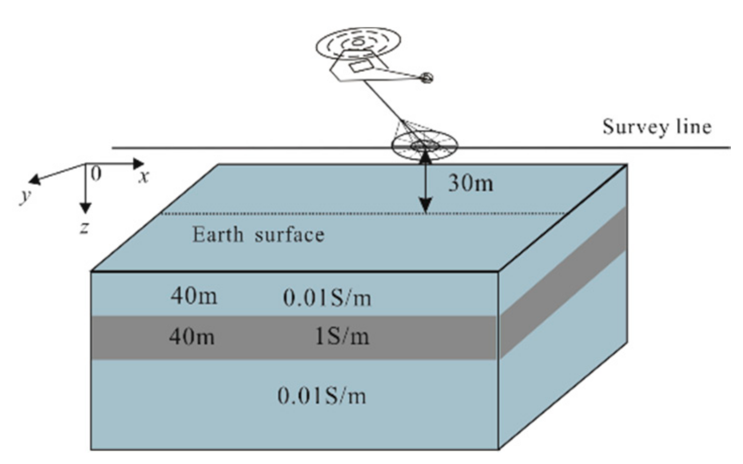
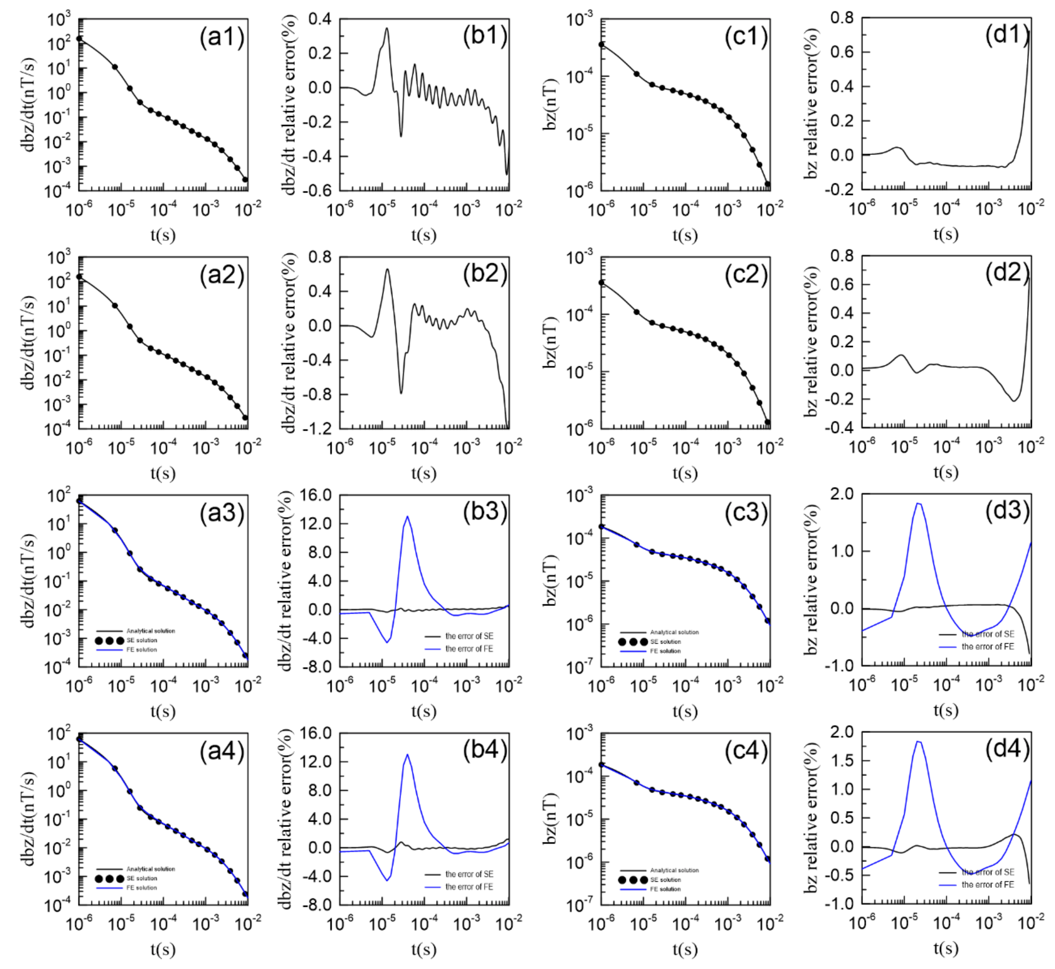
To verify the accuracy of our 3D AEM forward modeling algorithm, we use our SETD method to calculate the EM responses for a layered earth model and compare the results with 1D semi-analytical solutions [2]. The computational environment for our modeling is an Intel(R) Xeon(R) CPU E5-2650 v3 @ 2.30 GHz (double processors). The layered model is as follows: the first layer has a conductivity of 0.01 S/m and a thickness of 40 m; the second layer has a conductivity of 1 S/m and a thickness of 40 m; the underlying half-space has a conductivity of 0.01 S/m; the air layer’s conductivity is assumed to be 10⁻⁸ S/m. The AEM system takes a concentric configuration with a unit dipole moment. The altitudes of the transmitting and receiving coils are 30 m. Figure 1 shows the model parameters. The transmitting current is a step wave. We divide the time into ten segments, with each being further divided into 100 small ones. The time intervals for each segment are respectively 1.0 × 10⁻⁷ s, 2.0 × 10⁻⁷ s, 4.0 × 10⁻⁷ s, 8.0 × 10⁻⁷ s, 1.6 × 10⁻⁶ s, 3.2 × 10⁻⁶ s, 6.4 × 10⁻⁶ s, 1.28 × 10⁻⁵ s, 2.56 × 10⁻⁵ s, 5.12 × 10⁻⁵ s. To demonstrate the advantage of SETD in the improvement of the modeling accuracy by either refining the mesh or enhancing the order of the interpolation basis functions, we design two schemes: (1) 40 m × 40 m × 20 m mesh combined with the third order of interpolation basis functions, (2) 60 m × 60 m × 20 m mesh combined with the fourth order of interpolation basis functions. Figure 2(a1)–(d1),(a2)–(d2) show the dbz/dt and bz responses and the relative errors against the semi-analytical solutions. It is seen from the figure that the EM fields dbz/dt and bz for the two combined schemes decay steadily with time, the overall errors are less than 1.2%. This demonstrates that our SETD algorithm has high accuracy. In order to further illustrate the high-precision characteristics of the algorithm presented in this paper, we compare the solutions of our SE method with those of the finite-element algorithm based on structured grids [47]. Figure 2(a3)–(d3),(a4)–(d4) shows the relative errors of both methods against the semi-analytical solutions. It is clearly seen that our SE method has much higher accuracy than the finite-element method based on structured grids.

3.2. Influence Factors of Modeling Accuracy

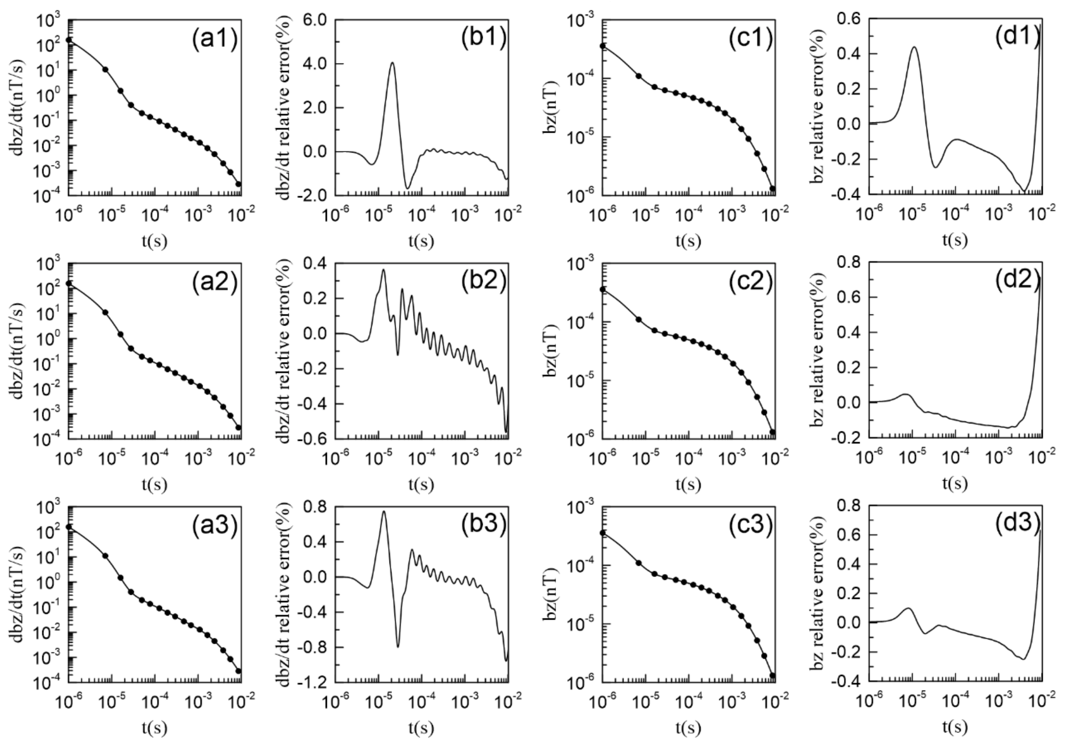
To explore the factors that affect the accuracy of our SETD algorithm, we simulate again the 3-layer model shown in Figure 1. The order of the interpolation basis functions and the mesh size for Figure 3(a1)–(d3) are variable. Analysis on Figure 3(a1)–(d1),(a2)–(d2) shows that when the order of the interpolation functions is fixed, the modeling accuracy is improved by refining the mesh. In contrast, the analysis on Figure 3 (a2)–(d2),(a3)–(d3) shows that when the size of the mesh is fixed, increasing the order of the interpolation functions can improve the accuracy as well. This implies that using SETD method for AEM forward modeling, one can improve the accuracy by either refining the mesh or increasing the order of the interpolation functions.

3.3. EM Responses for Typical Models

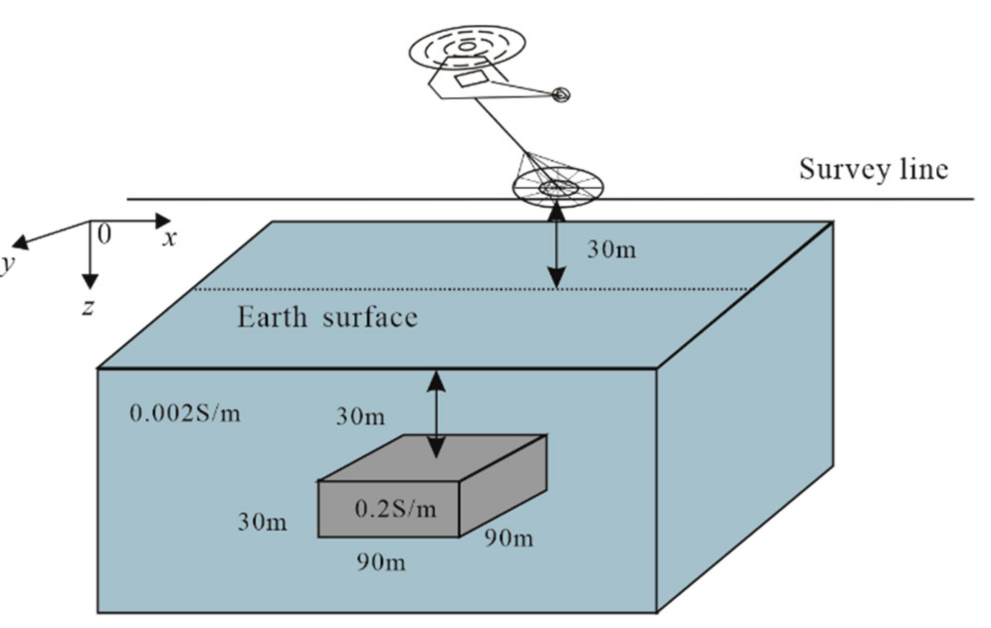
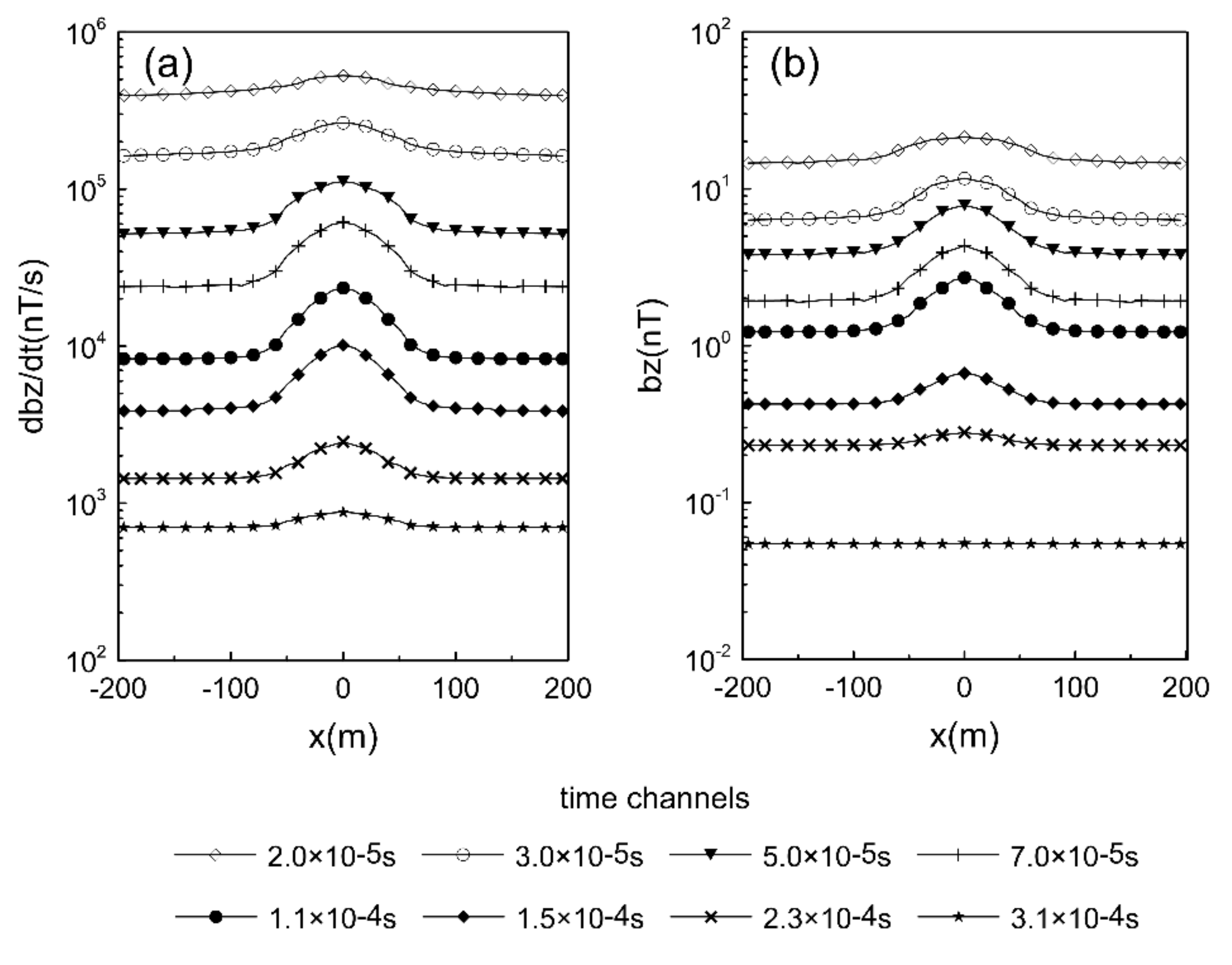
To analyze the characteristics of AEM responses in time-domain, we design the models of a horizontal plate, a vertical dyke, two vertical dykes in a homogeneous half-space. Figure 4 shows the horizontal dyke model with a dimension of 90 m × 90 m × 30 m, buried at a depth of 30 m and centered at (0,0,45 m). The conductivity of the dyke is 0.2 S/m, the background conductivity is 0.002 S/m. We model a flight system with a concentric configuration at an altitude of 30 m. The transmitting current is a step wave. The mesh size is 30 m × 30 m × 30 m and the third order of interpolation basis functions are used. Figure 5a,b show dbz/dt and bz responses for the horizontal plate. It is seen that (1) the existence of the conductive horizontal plate produces a symmetric and broad single-peak anomaly; (2) at early time, the EM field diffuses mainly in the upper resistive half-space, so that the EM signal is weak and broad; (3) with time passing, the EM field diffuses into the location of the conductive plate, so that strong EM signal is observed; (4) at later time, the EM field diffuses again into deep resistive earth, so that the EM signal becomes weak and broad again; (5) from the locations of half-peaks we can roughly determine the boundaries of the horizontal plate. For the computer environment mentioned in Section 3.1, the time for calculating a decay curve of 1000 time channels at a single survey station takes about 41.4 min.

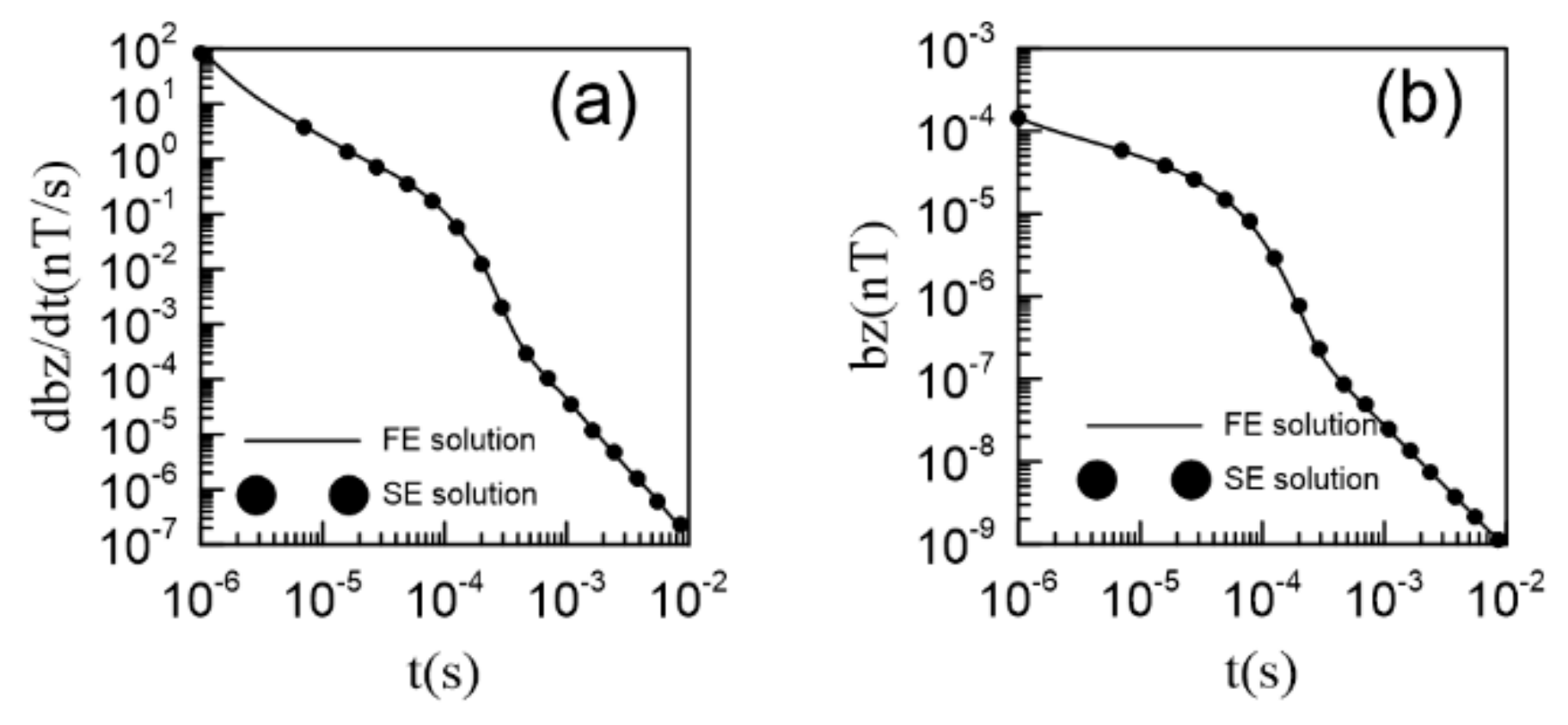
To further demonstrate the high accuracy of our SETD algorithm for 3D AEM modeling, we also use the FE method based on unstructured grids proposed by Qi et al. to calculate the EM responses for the model in Figure 4 at a single survey point [45]. The comparison of these two results is shown in Figure 6. It can obviously be seen that the results of the two methods agree well with each other, which again illustrates that our SETD algorithm has high modeling accuracy.

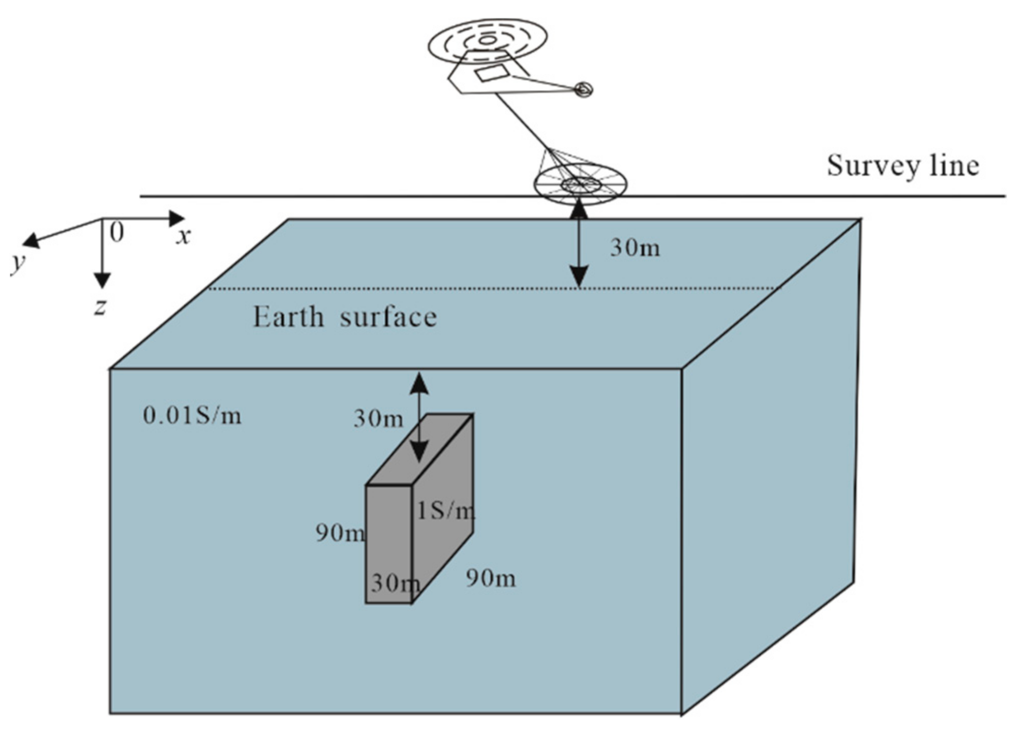
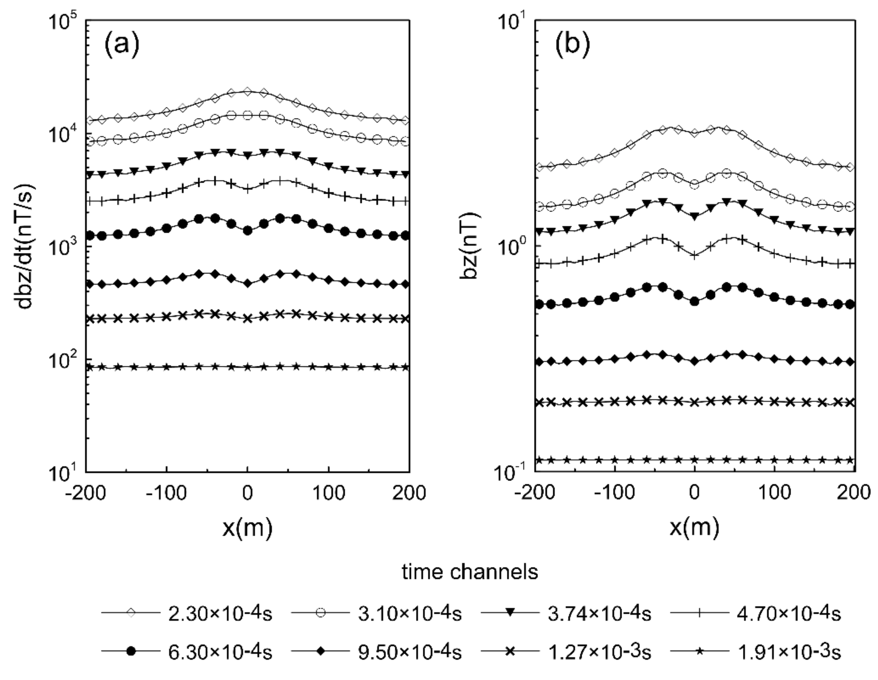
Furthermore, we study the AEM responses for a vertical dyke model. Refer to Figure 7, the vertical dyke has a dimension of 30 m × 90 m × 90 m and is buried at the depth of 30 m. The center is located at (0,0,75). The conductivities of the abnormal body and the background are 1 S/m and 0.01 S/m, respectively. The model domain is discretized into a mesh of 30 m × 30 m × 30 m. We use the fourth order of interpolation basis functions for the modeling. Figure 8a,b shows the dbz/dt and bz responses for the vertical dyke model. It is seen that (1) the EM responses at the early time is similar to those in Figure 5. Since the EM wave at early time has high-frequency content, the vertical dyke appears as a thick dyke, so that we see a single-peak anomaly; (2) with time passing, the EM field diffuses into the location of the dyke, the influence of the dyke becomes more obvious. In opposite to a horizontal plate, the EM responses for a vertical dyke shows two peaks. There exists a minimum over the top of the dyke due to zero coupling between the transmitter-receiver pair and the dyke; (3) at later time, the EM field passes through the dyke, the EM signal diffuses into the underlying half-space and becomes broader and weaker; (4) the center of the dyke can be determined by the minimum location of the EM responses, while the boundaries of the dyke can be roughly estimated from the middle points between the maximum and minimum peaks. This helps identify the underground targets from the AEM anomalies. For the computer environment mentioned in Section 3.1, the time for calculating a decay curve of 1000 time channels at a single survey station takes about 36.5 min.

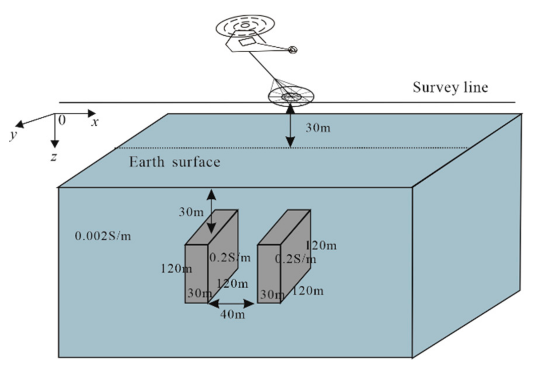
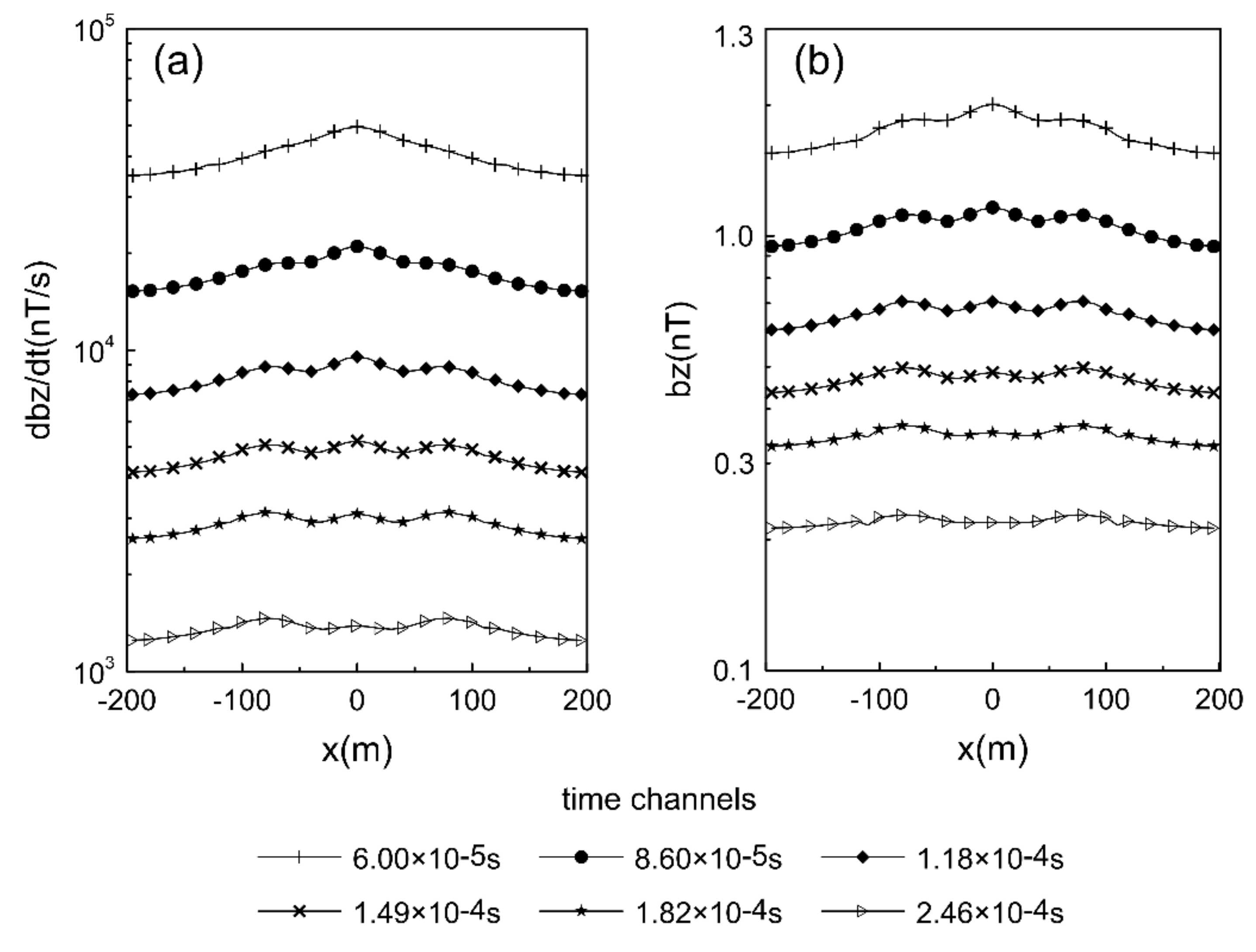
Next, we study the AEM responses for a model with two vertical dykes embedded in a homogeneous half-space (Figure 9). Each dyke has a dimension of 30 m × 120 m × 120 m and is buried at the depth of 30 m. The distance between the two dykes is 40 m. The conductivities of the two dykes are 0.2 S/m, while the background conductivity is 0.002 S/m. We discretize the model domain into the elements of 30 m × 30 m × 30 m and take the fourth order of interpolation basis functions. Figure 10a,b show the dbz/dt and bz responses. It is seen from the figures that the EM responses demonstrate as the superposition of two dykes. At the early time, the EM field shows a weak and broad anomaly, meaning that the two dykes are coupled and not distinguishable. With time passing the anomalies from two dykes become stronger and more distinguishable. Three peaks can be seen clearly, representing the EM field of two dykes. The anomaly in the middle is larger than the neighboring two anomalies as it is the superposed anomaly from the two dykes. Similarly, the centers and the boundaries of the dykes can be distinguished respectively from the minimum anomaly locations and the middle points between the maximum and minimum peaks. This further implies that from the anomalies of a time-domain AEM system, we can distinguish the anomalous bodies in the underground. For the computer environment mentioned in Section 3.1, the time for calculating a decay curve of 1000 time channels at a single survey station takes about 43.7 min.

4. Conclusions

In this paper, we have successfully developed and applied the SETD method to 3D AEM forward modeling in time-domain. Using the high-order of GLC interpolation basis functions, we can calculate analytically the stiffness and mass matrices for AEM forward problem and achieve high numerical accuracy. The backward Euler scheme for the time discretization, resulting in an unconditionally stable equation for EM fields, further improves the stability and accuracy of our 3D time-domain AEM forward modeling. Comparisons with the semi-analytical solutions for a layered earth model and with the finite-element solutions for 3D models demonstrated that our SETD method has high accuracy. In addition, the modeling accuracy of our SE method can be improved by either refining the mesh or increasing the order of the interpolation basis functions. This offers more possibilities for us to achieve accurate results in time-domain AEM modeling. Numerical experiments on typical models show that the geometries and locations of the abnormal bodies in the underground can be identified from the AEM signal.

It must be pointed out that we have in this paper only used the regular hexahedral meshes in our SE modeling, so that we cannot yet model the complex underground structures and topography. Moreover, the modeling efficiency of our algorithm is not yet satisfying that will surely restrict its application in AEM inversions. All these will be our future research focus.

References

- Steuer, A.; Siemon, B.; Auken, E. A comparison of helicopter-borne electromagnetics in frequency- and time-domain at the Cuxhaven valley in Northern Germany. J. Appl. Geophys. 2009, 67, 194–205. [Google Scholar] [CrossRef]
- Yin, C.C. Airborne Electromagnetic Theory and Exploration Technology; Science Press: Beijing, China, 2018. [Google Scholar]
- Beamish, D. An assessment of inversion methods for AEM data applied to environmental studies. J. Appl. Geophys. 2002, 51, 75–96. [Google Scholar] [CrossRef] [Green Version]
- Smith, R. Airborne electromagnetic methods: Applications to minerals, water and hydrocarbon exploration. Recorder 2010, 35, 7–10. [Google Scholar]
- Li, J.; Liu, Y.-H.; Yin, C.; Ren, X.; Su, Y. Fast imaging of time-domain airborne EM data using deep learning technology. Geophysics 2020, 85, E163–E170. [Google Scholar] [CrossRef]
- Yin, C.; Hodges, G. Simulated Annealing for Airborne EM Inversion. In Proceedings of the 69th EAGE Conference and Exhibition Incorporating SPE EUROPEC 2007, London, UK, 11–14 June 2007; European Association of Geoscientists & Engineers: Utrecht, The Netherlands. [Google Scholar]
- Hodges, G. Practical inversions for helicopter electromagnetic data. In Proceedings of the 15th Annual Symposium on the Application of Geophysics to Environmental and Engineering Problems (SAGEEP), San Antonio, TX, USA, 6–10 April 2010; Environmental & Engineering Geophysical Society: Denver, CO, USA, 2003; pp. 45–58. [Google Scholar]
- Yee, K. Numerical solution of initial boundary value problems involving Maxwell’s equations in isotropic media. IEEE Trans. Antennas Propag. 1966, 14, 302–307. [Google Scholar]
- Madden, T.; Mackie, R. Three-dimensional magnetotelluric modelling and inversion. Proc. IEEE 1989, 77, 318–333. [Google Scholar] [CrossRef]
- Newman, G.A.; Alumbaugh, D.L. Frequency-domain modelling of airborne electromagnetic responses using staggered finite differences1. Geophys. Prospect. 1995, 43, 1021–1042. [Google Scholar] [CrossRef]
- Liu, Y.; Yin, C. 3D anisotropic modeling for airborne EM systems using finite-difference method. J. Appl. Geophys. 2014, 109, 186–194. [Google Scholar] [CrossRef]
- Tang, J.-T.; Ren, Z.-Y.; Hua, X.-R. The forward modeling and inversion in geophysical electromagnetic field. Prog. Geophys. 2007, 22, 1181–1194. [Google Scholar]
- Hohmann, G.W. Electromagnetic scattering by conductors in the earth near a line source of current. Geophysics 1971, 36, 101–131. [Google Scholar] [CrossRef]
- Peltoniemi, M.; Bärs, R.; Newman, G.A. Numerical modelling of airborne electromagnetic anomalies originating from low-conductivity 3D bodies1. Geophys. Prospect. 1996, 44, 55–69. [Google Scholar] [CrossRef]
- Cox, L.H.; Wilson, G.A.; Zhdanov, M.S. 3D inversion of airborne electromagnetic data using a moving footprint. Explor. Geophys. 2010, 41, 250–259. [Google Scholar] [CrossRef]
- Yin, C.; Lu, Y.; Liu, Y.; Zhang, B.; Qi, Y.; Cai, J. Multigrid quasi-linear approximation for three-dimensional airborne EM forward modeling. J. Jilin Univ. 2018, 48, 252–260. [Google Scholar]
- Coggon, J.H. Electromagnetic and electrical modeling by the finite element method. Geophysics 1971, 36, 132–155. [Google Scholar] [CrossRef]
- Wannamaker, P.E.; Stodt, J.A.; Rijo, L. Two-dimensional topographic responses in magnetotelluric modeled using finite ele-ments. Geophysics 1986, 51, 2131–2144. [Google Scholar] [CrossRef]
- Unsworth, M.J.; Travis, B.J.; Chave, A.D. Electromagnetic induction by a finite electric dipole source over a 2-D earth. Geophysics 1993, 58, 198–214. [Google Scholar] [CrossRef]
- Key, K.; Weiss, C. Adaptive finite-element modeling using unstructured grids: The 2D magnetotelluric example. Geophysics 2006, 71, G291–G299. [Google Scholar] [CrossRef]
- Ren, Z.; Tang, J. 3D direct current resistivity modeling with unstructured mesh by adaptive finite-element method. Geophysics 2010, 75, H7–H17. [Google Scholar] [CrossRef]
- Ren, Z.; Kalscheuer, T.; Greenhalgh, S.; Maurer, H. A goal-oriented adaptive finite-element approach for plane wave 3D elec-tromagnetic modeling. Geophys. J. Int. 2013, 194, 700–718. [Google Scholar] [CrossRef] [Green Version]
- Zhang, B.; Yin, C.; Liu, Y.; Cai, J. 3D modeling on topographic effect for frequency-/time-domain airborne EM systems. Chin. J. Geophys. 2016, 59, 1506–1520. [Google Scholar]
- Yin, C.; Qi, Y.; Liu, Y.; Cai, J. 3D time-domain airborne EM forward modeling with topography. J. Appl. Geophys. 2016, 134, 11–22. [Google Scholar] [CrossRef]
- Haber, E.; Ascher, U.M. Fast Finite Volume Simulation of 3D Electromagnetic Problems with Highly Discontinuous Coefficients. SIAM J. Sci. Comput. 2001, 22, 1943–1961. [Google Scholar] [CrossRef]
- Haber, H.; Schwarzbach, C. Parallel inversion of large-scale airborne time-domain electromagnetic data with multiple OcTree meshes. Inverse Probl. 2014, 30, 055011. [Google Scholar] [CrossRef]
- Haber, E.; Ruthotto, L. A multiscale finite volume method for Maxwell’s equations at low frequencies. Geophys. J. Int. 2014, 199, 1268–1277. [Google Scholar] [CrossRef]
- Jahandari, H.; Farquharson, C.G. A finite-volume solution to the geophysical electromagnetic forward problem using un-structured grids. Geophysics 2014, 79, E287–E302. [Google Scholar] [CrossRef]
- Patera, A.T. A spectral element method for fluid dynamics: Laminar flow in a channel expansion. J. Comput. Phys. 1984, 54, 468–488. [Google Scholar] [CrossRef]
- Black, K. A conservative spectral element method for the approximation of compressible fluid flow. Kybern. Praha. 1999, 35, 133–146. [Google Scholar]
- Frutos, J.D.; Novo, J. A Spectral Element Method for the Navier--Stokes Equations with Improved Accuracy. Siam J. Numer. Anal. 2000, 38, 799–819. [Google Scholar] [CrossRef]
- Komatitsch, D.; Vilotte, J.P.; Vai, R.; José, M.C.C.; Sa′nchez-Sesma, F.J. The spectral element method for elastic wave equations—Application to 2-D and 3-D seismic problems. Int. J. Numer. Methods Eng. 1999, 45, 1139–1164. [Google Scholar] [CrossRef]
- Komatitsch, D.; Tromp, J. Spectral-element simulations of global seismic wave propagation—I. Validation. Geophys. J. Int. 2002, 149, 390–412. [Google Scholar] [CrossRef]
- Komatitsch, D.; Tromp, J. Spectral-element simulations of global seismic wave propagation-II. Three-dimensional models, oceans, rotation and self-gravitation. Geophys. J. Int. 2002, 150, 303–318. [Google Scholar] [CrossRef]
- Chaljub, E.; Komatitsch, D.; Vilotte, J.-P.; Capdeville, Y.; Valette, B.; Festa, G. Spectral-element analysis in seismology. Adv. Geophys. 2007, 48, 365–419. [Google Scholar] [CrossRef]
- Wang, T.; Li, R.; Li, X.; Zhang, M.; Long, G. Numerical spectral element modeling for seismic wave propagation in transversely isotropic medium. Prog. Geophys. 2007, 22, 778–784. [Google Scholar]
- Yin, C.; Huang, X.; Liu, Y.; Cai, J. 3-D Modeling for Airborne EM using the Spectral-element Method. J. Environ. Eng. Geophys. 2017, 22, 13–23. [Google Scholar] [CrossRef]
- Huang, X.; Yin, C.; Cao, X.-Y.; Liu, Y.-H.; Zhang, B.; Cai, J. 3D anisotropic modeling and identification for airborne EM systems based on the spectral-element method. Appl. Geophys. 2017, 14, 419–430. [Google Scholar] [CrossRef]
- Liu, L.; Yin, C.; Liu, Y.; Qiu, C.; Huang, X.; Zhang, B. Spectral element method for 3D frequency-domain marine con-trolled-source electromagnetic forward modeling. Chin. J. Geophys. 2018, 61, 756–766. [Google Scholar]
- Knight, J.H.; Raiche, A.P. Transient electromagnetic calculations using the Gaver-Stehfest inverse Laplace transform method. Geophysics 1982, 47, 47–50. [Google Scholar] [CrossRef]
- Yin, C.; Huang, W.; Ben, F. The full-time electromagnetic modeling for time-domain airborne electromagnetic systems. Chin. J. Geophys. 2003, 56, 3153–3162. [Google Scholar]
- Qiu, C.; Güttel, S.; Ren, X.; Yin, C.; Liu, Y.; Zhang, B.; Egbert, G. A block rational Krylov method for 3-D time-domain marine controlled-source electromagnetic modelling. Geophys. J. Int. 2019, 218, 100–114. [Google Scholar] [CrossRef]
- Jin, J.M. The Finite Element Method in Electromagnetics; Wiley: Hoboken, NJ, USA, 2002. [Google Scholar]
- Ascher, U.M.; Petzold, L.R. Computer Methods for Ordinary Differential Equations and Differential-Algebraic Equations. Comput. Methods Ordinary Differ. Equ. Differ. Algebraic Equ. 1998. [Google Scholar] [CrossRef]
- Qi, Y.-F.; Yin, C.-C.; Liu, Y.-H.; Cai, J. 3D time-domain airborne EM full-wave forward modeling based on instantaneous current pulse. Chin. J. Geophys. 2017, 60, 369–382. [Google Scholar]
- Ilić, M.M.; Notaros, B. Higher order hierarchical curved hexahedral vector finite elements for electromagnetic modeling. IEEE Trans. Microw. Theory Tech. 2003, 51, 1026–1033. [Google Scholar] [CrossRef]
- Huang, W.; Ben, F.; Yin, C. Three-dimensional anisotropic modeling for time-domain airborne electromagnetics. Appl. Geophys. 2017, 14, 431–440. [Google Scholar] [CrossRef]
Figure 1.
Airborne electromagnetic (AEM) system over a 3-layer earth.
Figure 2.
dbz/dt and bz responses and relative errors against the semi-analytical solutions for the 3-layer model in Figure 1. (a1)–(d1) Scheme 1: 40 m × 40 m × 20 m mesh combined with the third order of interpolation basis functions; (a2)–(d2) Scheme 2: 60 m × 60 m × 20 m mesh combined with the fourth order of interpolation basis functions; (a3)–(d3) Comparison of the finite-element solutions based on structured grids with the spectral element solutions via Scheme 1; (a4)–(d4) Comparison of the finite-element solutions with the spectral element solutions via Scheme 2. The central grid size for the finite-element method is 2 m × 2 m × 2 m.
Figure 3.
dbz/dt and bz responses and relative errors against the semi-analytical solutions for the combinations of different mesh size and the orders of the interpolation functions. (a1)–(d1) third order of interpolation functions combined with the mesh size of 20 m × 20 m × 20 m; (a2)–(d2) third order of interpolation functions combined with the mesh size of 20 m × 20 m × 10 m; (a3)–(d3) fourth order of interpolation functions combined with the mesh size of 20 m × 20 m × 20 m. Note that the modeling accuracy can be improved by either refining the mesh or increasing the order of the interpolation functions.
Figure 4.
A horizontal plate embedded in a homogeneous half-space.
Figure 5.
(a) dbz/dt and (b) bz responses for the horizontal plate model in Figure 4.
Figure 6.
Comparison of (a) dbz/dt and (b) bz responses calculated by our SETD method with those calculated by FE method based on unstructured grids for the horizontal plate model in Figure 4.
Figure 7.
A vertical dyke embedded in a homogeneous half-space.
Figure 8.
(a) dbz/dt and (b) bz responses for the vertical dyke model in Figure 7.
Figure 9.
Two vertical dykes embedded in a homogeneous half-space.
Figure 10.
(a) dbz/dt and (b) bz responses for the vertical dyke model in Figure 9.
Publisher’s Note: MDPI stays neutral with regard to jurisdictional claims in published maps and institutional affiliations. |
© 2021 by the authors. Licensee MDPI, Basel, Switzerland. This article is an open access article distributed under the terms and conditions of the Creative Commons Attribution (CC BY) license (http://creativecommons.org/licenses/by/4.0/).
Share and Cite
MDPI and ACS Style
Yin, C.; Gao, Z.; Su, Y.; Liu, Y.; Huang, X.; Ren, X.; Xiong, B. 3D Airborne EM Forward Modeling Based on Time-Domain Spectral Element Method. Remote Sens. 2021, 13, 601. https://0-doi-org.brum.beds.ac.uk/10.3390/rs13040601
AMA Style
Yin C, Gao Z, Su Y, Liu Y, Huang X, Ren X, Xiong B. 3D Airborne EM Forward Modeling Based on Time-Domain Spectral Element Method. Remote Sensing. 2021; 13(4):601. https://0-doi-org.brum.beds.ac.uk/10.3390/rs13040601
Chicago/Turabian StyleYin, Changchun, Zonghui Gao, Yang Su, Yunhe Liu, Xin Huang, Xiuyan Ren, and Bin Xiong. 2021. "3D Airborne EM Forward Modeling Based on Time-Domain Spectral Element Method" Remote Sensing 13, no. 4: 601. https://0-doi-org.brum.beds.ac.uk/10.3390/rs13040601
Note that from the first issue of 2016, this journal uses article numbers instead of page numbers. See further details here.