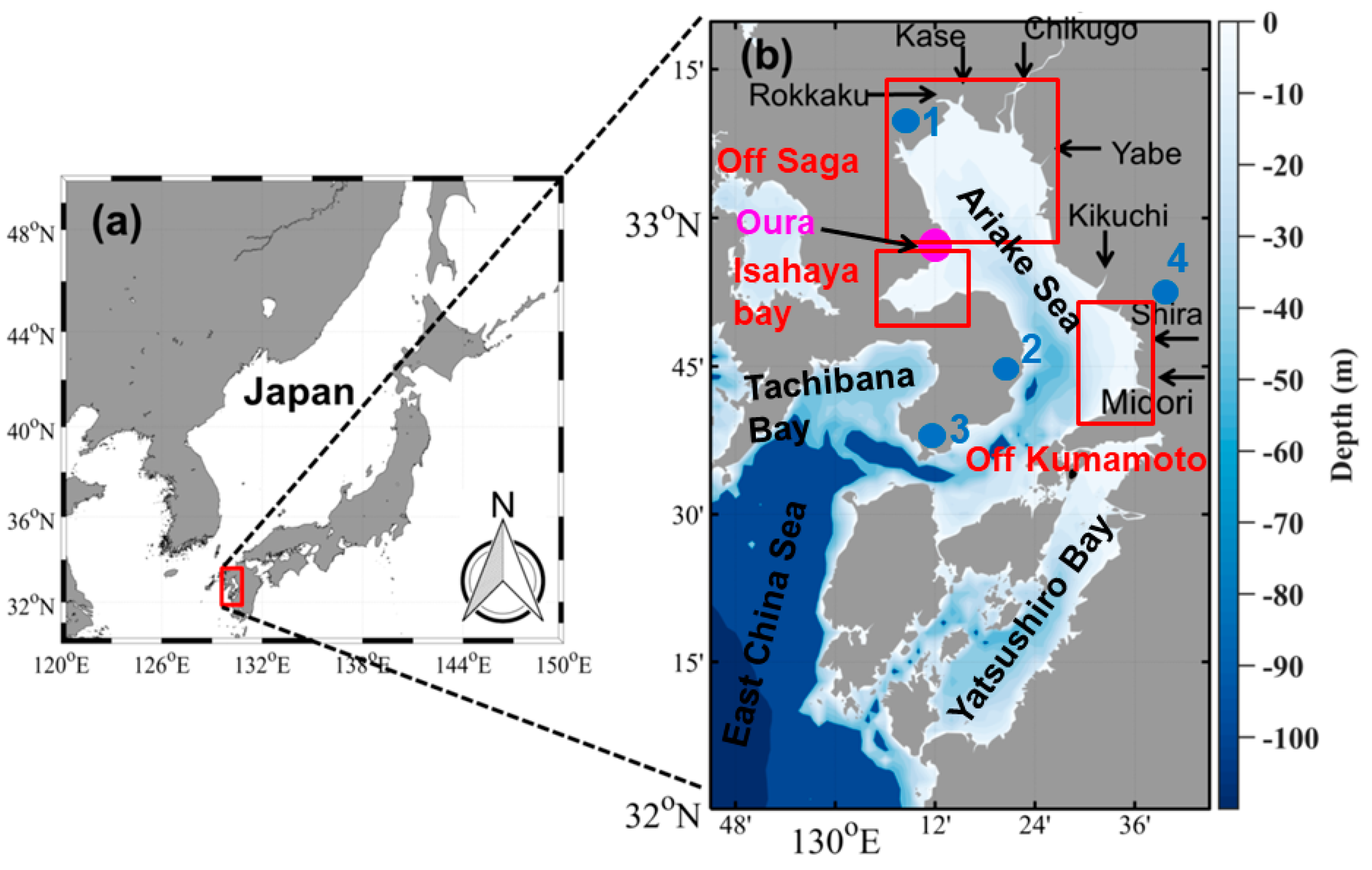
Figure 1.
Location of the Ariake Sea, Japan (a). The water depth of the bay is shown in light to dark blue (b). The seven main rivers of Rokkaku, Kase, Chikugo, Yabe, Kikuchi, Shira, Midori, and Kuma are indicated by arrows. The three regional areas, i.e., Off Saga, Isahaya Bay, and off Kumamoto, are highlighted by red boxes. The observation station for tidal level data of Ariake Sea, named Oura, is represented by a magenta filled circle. The four observation stations for sea level amplitude, wind speed, precipitation, and sea surface temperature, are represented by blue filled circles.
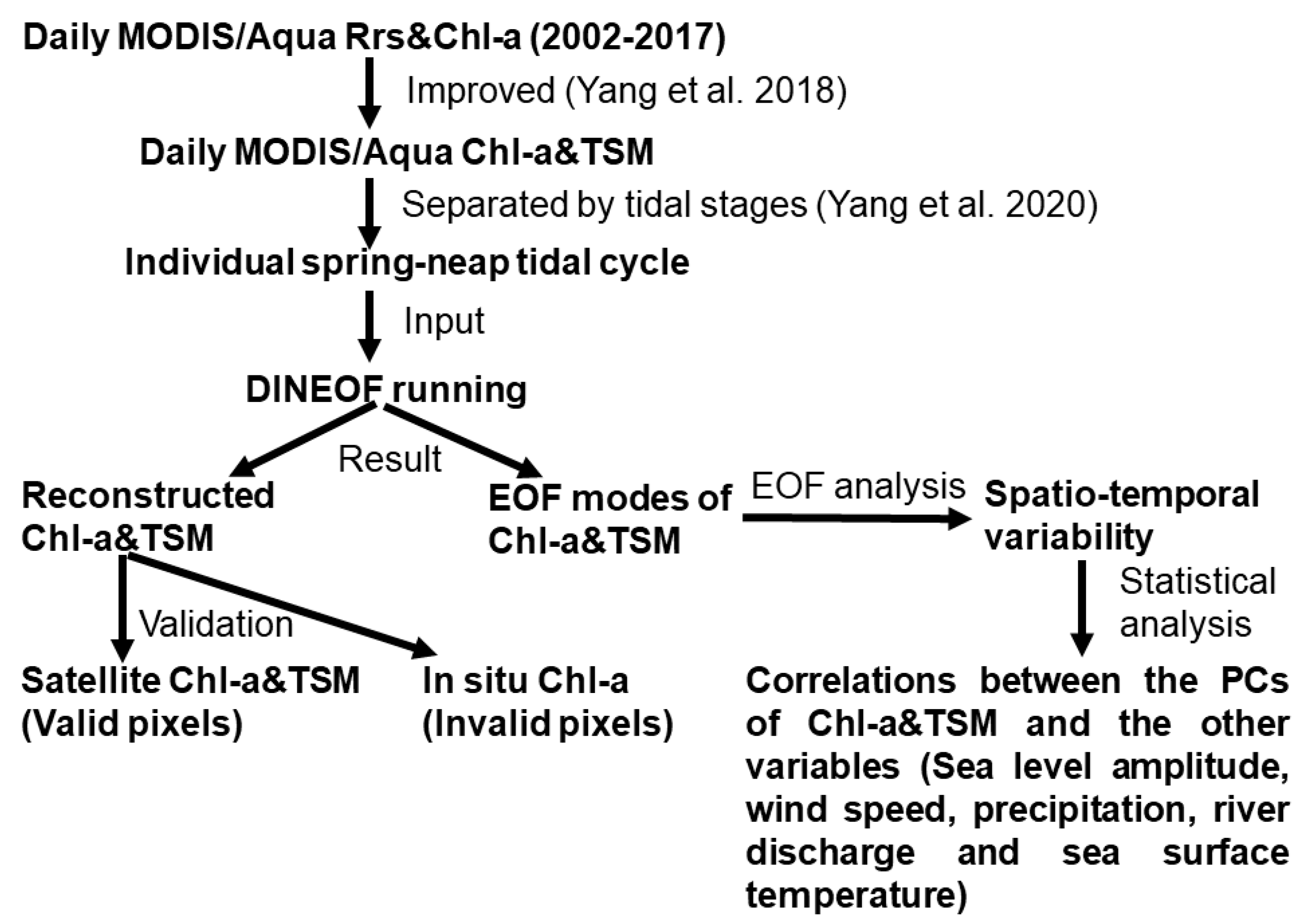
Figure 2.
Flow chart of the procedure of the methods.
Figure 2.
Flow chart of the procedure of the methods.
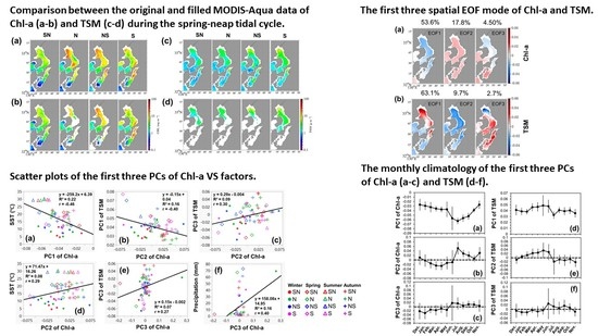
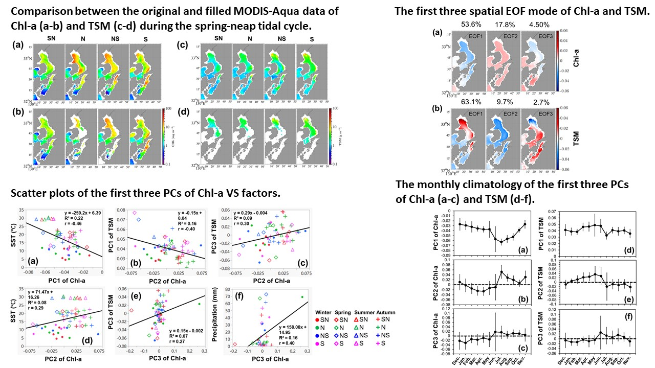
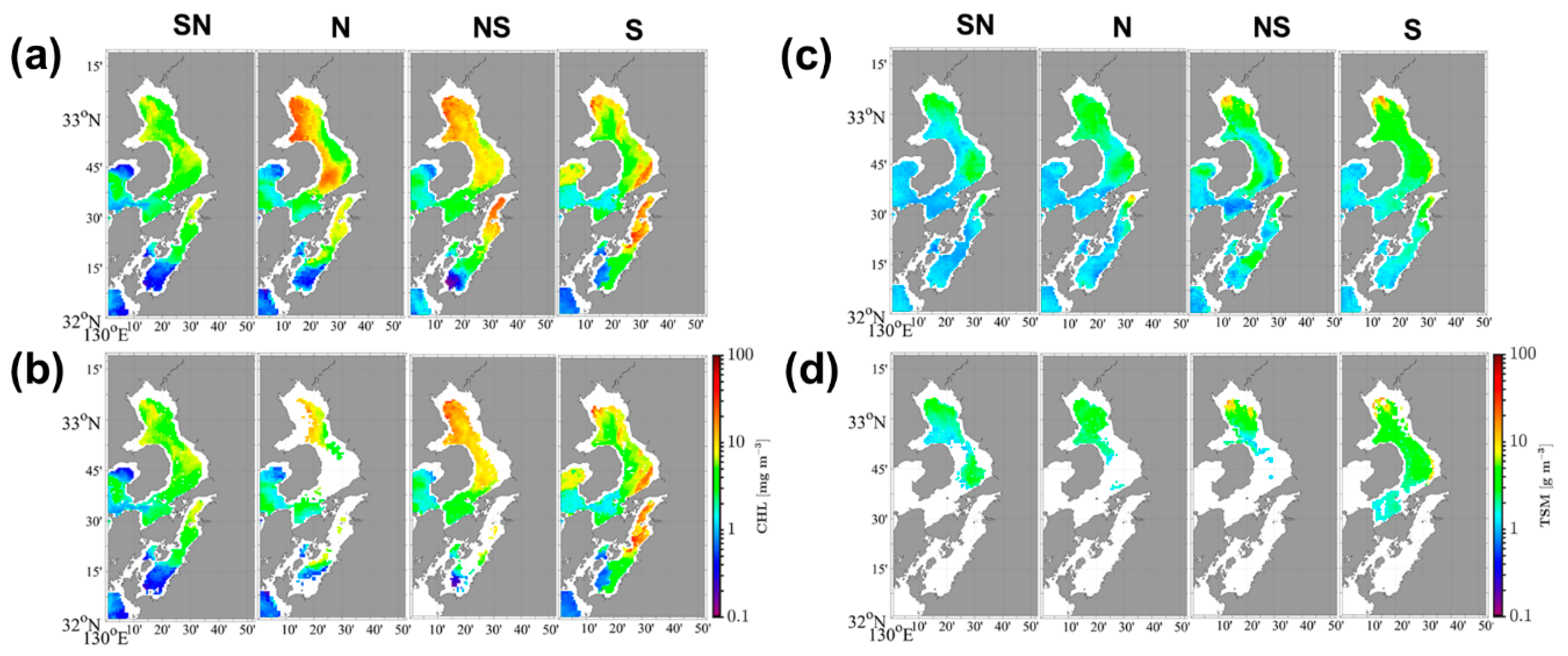
Figure 3.
Satellite images of reconstructed and original chlorophyll-a (Chl-a) (a,b) and total suspended matter (TSM) (c,d) during the spring-neap tidal cycles from April 28 to May 10, 2005 and from January 21 to February 4, 2014, respectively. SN, N, NS, and S represent spring to neap, neap, neap to spring, and spring tide, respectively.
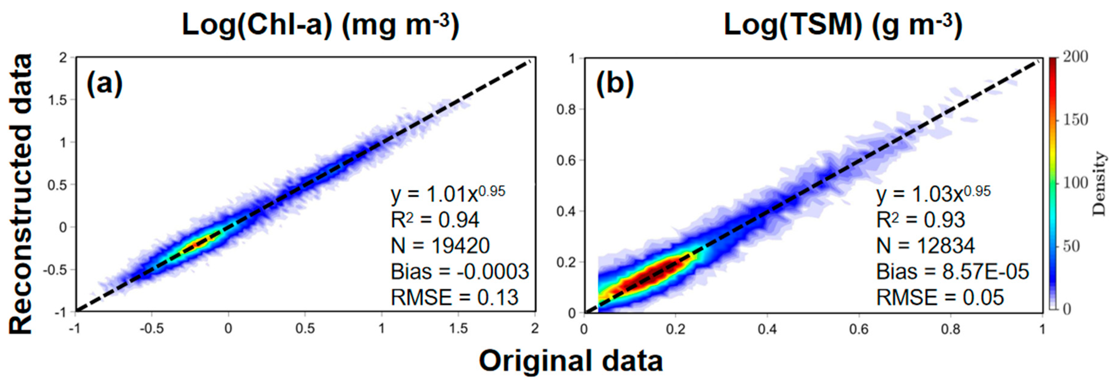
Figure 4.
Scatter plots of the reconstructed versus original Chl-a (a) and TSM (b) for the 1% randomly selected validation pixels from all Data INterpolating Empirical Orthogonal Functions (DINEOF) input datasets. The dotted line is the 1:1 line.
Figure 4.
Scatter plots of the reconstructed versus original Chl-a (a) and TSM (b) for the 1% randomly selected validation pixels from all Data INterpolating Empirical Orthogonal Functions (DINEOF) input datasets. The dotted line is the 1:1 line.
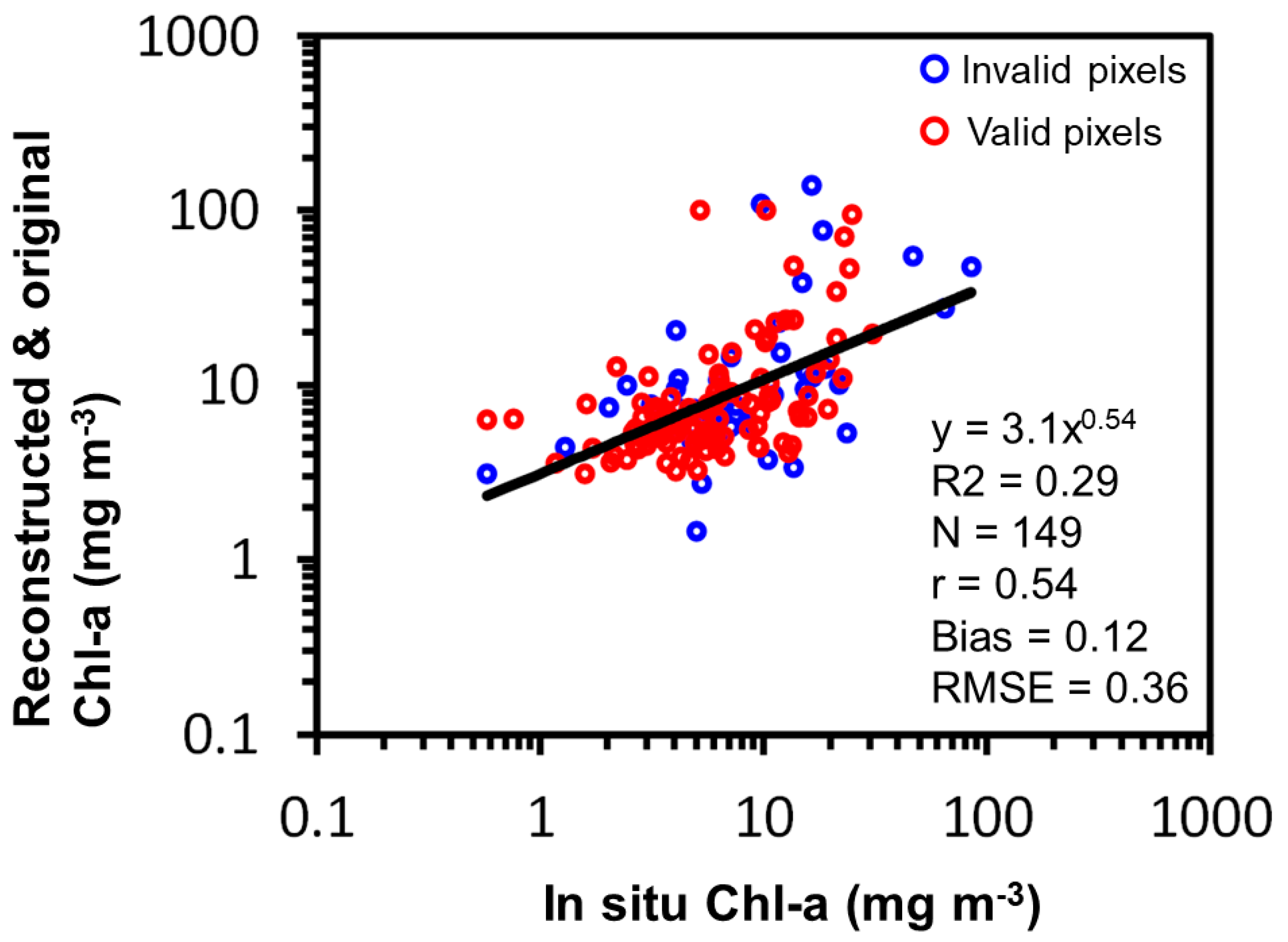
Figure 5.
Scatter plot of the original and reconstructed Chl-a from the pixels with valid and invalid values in the original satellite images, respectively, versus the in situ Chl-a for all the satellite in situ matchups. The blue and red symbols represent the constructed versus in situ Chl-a and the original versus in situ Chl-a, respectively.
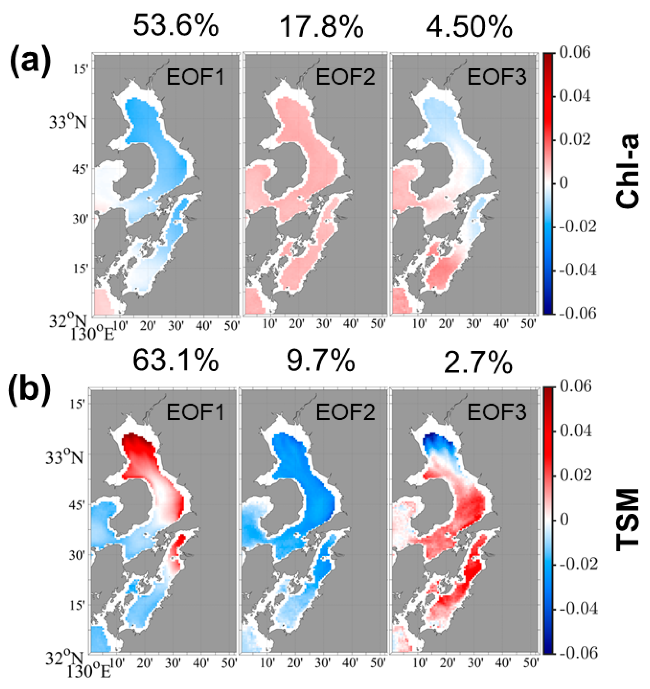
Figure 6.
Spatial EOF maps of Chl-a (a) and TSM (b) for the first three EOF modes. The explained variance of each mode is shown above each map.
Figure 6.
Spatial EOF maps of Chl-a (a) and TSM (b) for the first three EOF modes. The explained variance of each mode is shown above each map.
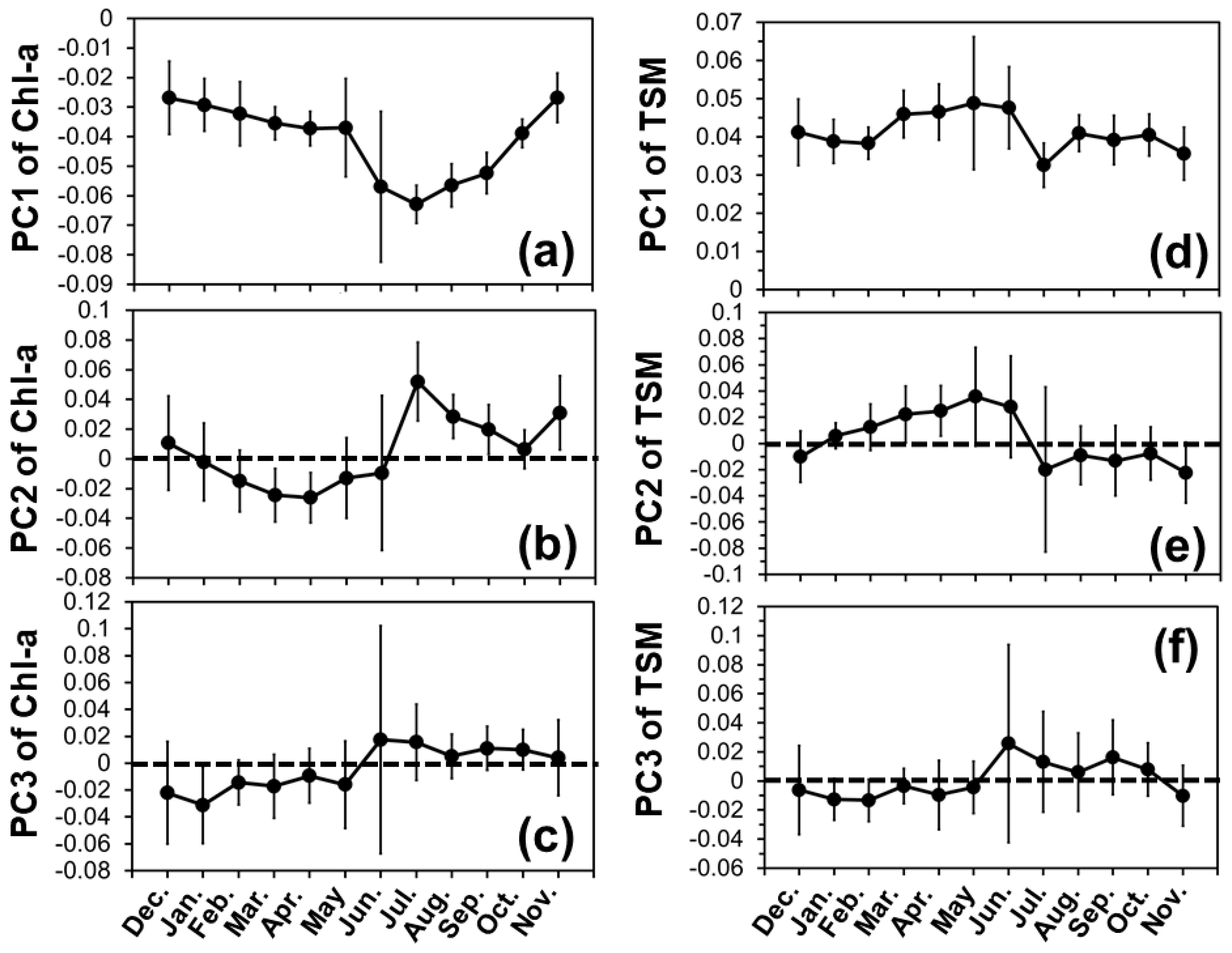
Figure 7.
Monthly temporal functions, i.e., PCs, of Chl-a (a–c) and TSM (d–f) corresponding to the first three EOF modes. The dotted lines and vertical bars represent y = 0 and one standard deviation, respectively.
Figure 7.
Monthly temporal functions, i.e., PCs, of Chl-a (a–c) and TSM (d–f) corresponding to the first three EOF modes. The dotted lines and vertical bars represent y = 0 and one standard deviation, respectively.
Figure 8.
Monthly sea level amplitude (a), wind speed (b), precipitation (c), sea surface temperature (d), and river discharge (e). The vertical bars represent one standard deviation.
Figure 8.
Monthly sea level amplitude (a), wind speed (b), precipitation (c), sea surface temperature (d), and river discharge (e). The vertical bars represent one standard deviation.
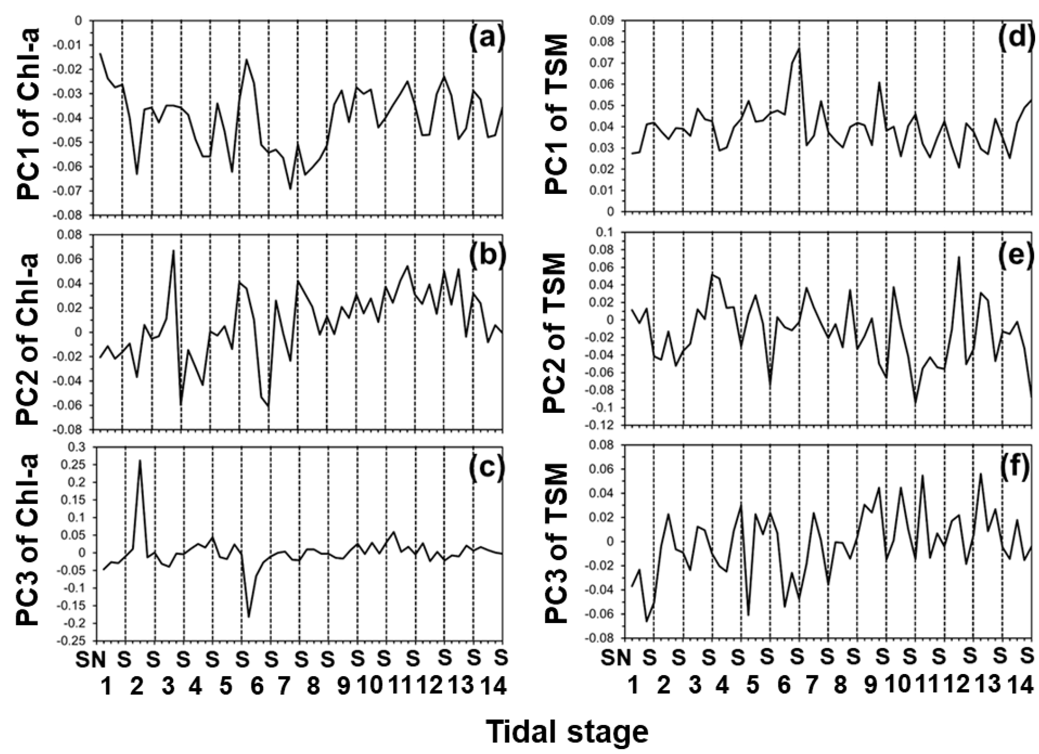
Figure 9.
The fourteen individual events of the spring-neap tidal cycle of temporal functions, i.e., PCs, of Chl-a (a–c) and TSM (d–f) corresponding to the first three EOF modes. The dotted lines are used to separate the tidal cycles. Each tidal cycle is divided into four tidal stages, i.e., spring to neap (SN), neap (N), neap to spring (NS), and spring (S) tides.
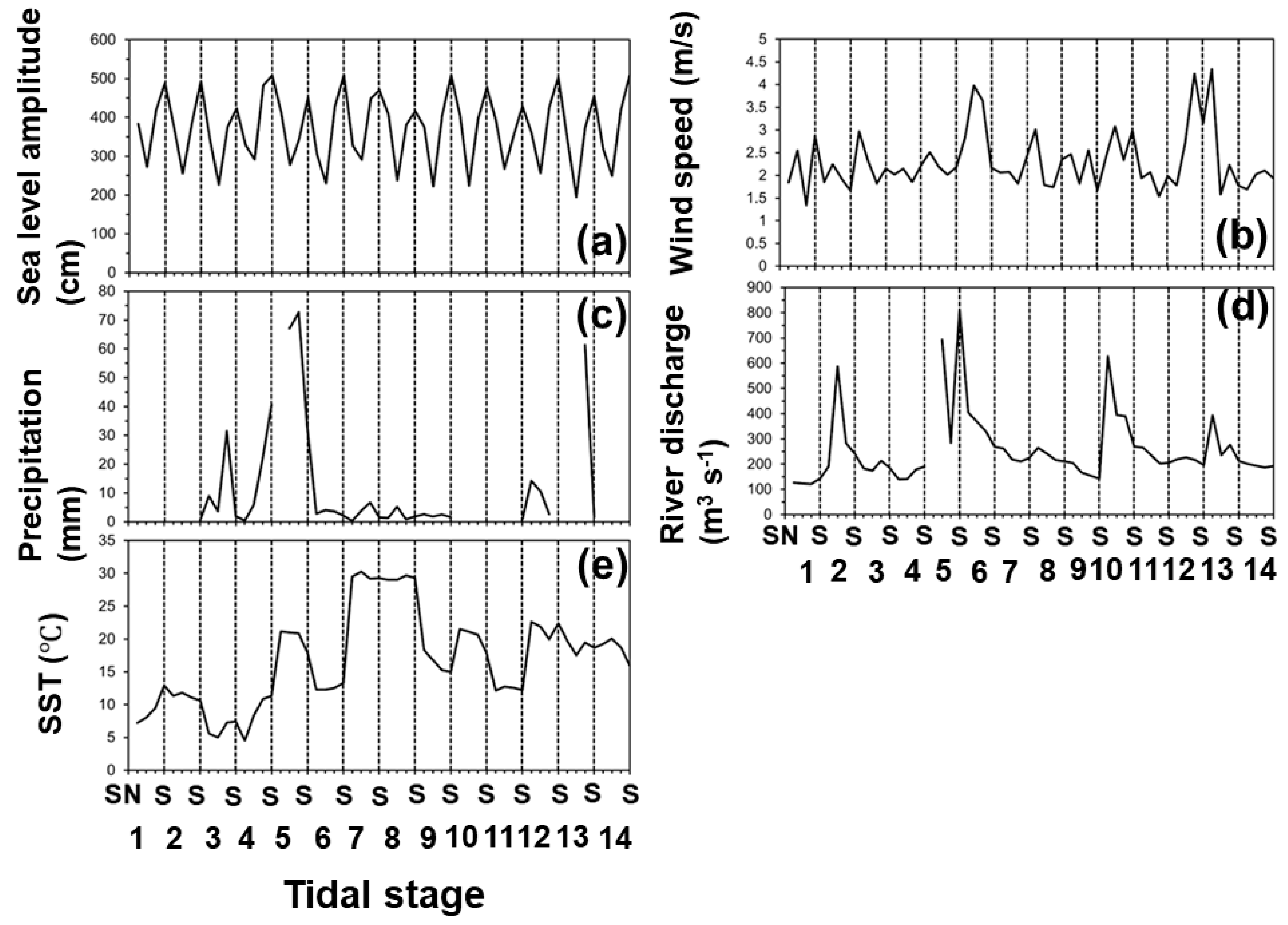
Figure 10.
The fourteen individual events of the spring-neap tidal cycle of the sea level amplitude (a), wind speed (b), precipitation (c), river discharge (d), and sea surface temperature (SST) (e). The dotted lines are used to separate the tidal cycles. Each tidal cycle is divided into four tidal stages, i.e., spring to neap (SN), neap (N), neap to spring (NS), and spring (S) tides.
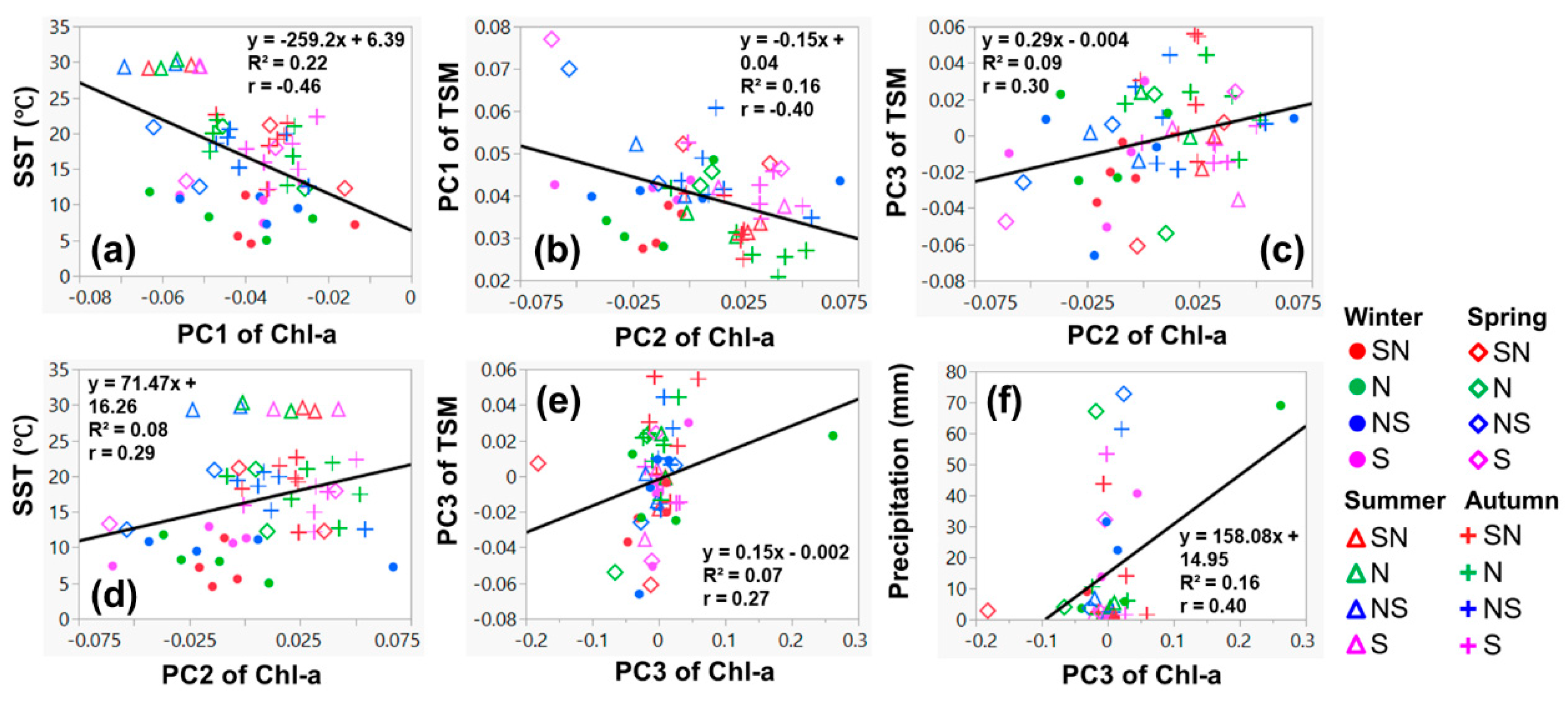
Figure 11.
Scatter plots of the PCs of Chl-a and factors for the significant correlations in
Table 5, i.e., PC1 of Chl-a vs. sea surface temperature (SST) (
a), PC2 of Chl-a vs. PC1 of TSM (
b), PC2 of Chl-a vs. PC3 of TSM (
c), PC2 of Chl-a vs. sea surface temperature (SST) (
d), PC3 of Chl-a vs. PC3 of TSM (
e), and PC3 of Chl-a vs. precipitation (
f). The data for winter, spring, summer, and autumn are represented by filled circle, diamond, triangle, and plus symbols, and the data for spring to neap (SN), neap (N), neap to spring (NS), and spring (S) tides are represented by red, green, blue, and magenta colors. The black lines in each plot are regression lines.
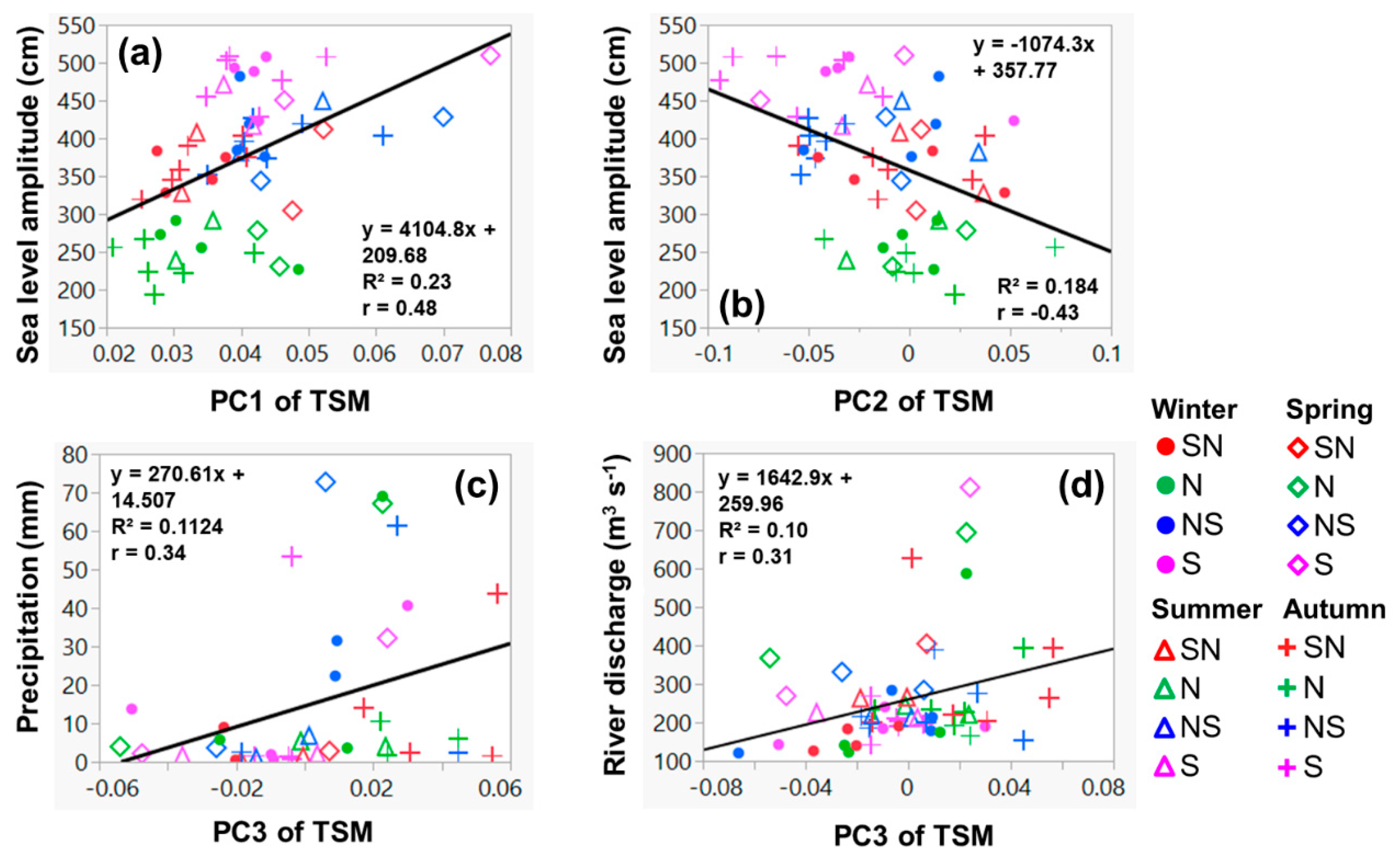
Figure 12.
Scatter plots of the PCs of TSM and factors for the significant correlations in
Table 6, i.e., PC1 of TSM vs. sea level amplitude (
a), PC2 of TSM vs. sea level amplitude (
b), PC3 of TSM vs. precipitation (
c), and PC3 of TSM vs. river discharge (
d). The data for winter, spring, summer, and autumn are represented by filled circle, diamond, triangle, and plus symbols, and the data for spring to neap (SN), neap (N), neap to spring (NS), and spring (S) tides are represented by red, green, blue, and magenta colors. The black lines in each plot are regression lines.
Table 1.
Descriptions of the flags used in this study.
Table 1.
Descriptions of the flags used in this study.
| Bit. | Name | Short Description |
|---|
| 01 | Land | Pixel is over land |
| 03 | HIGLINT | Sunglint: Reflectance exceeds the threshold |
| 04 | HILT | Observed radiance is very high or saturated |
| 05 | HISATZEN | Sensor view zenith angle exceeds the threshold |
| 09 | CLDICE | Probable cloud or ice contamination |
| 12 | HISOLZEN | Solar zenith exceeds the threshold |
| 14 | LOWLW | Very low water-leaving radiance |
| 19 | MAXAERITER | Maximum iterations reached for NIR iteration |
| 25 | NAVFAIL | Navigation failure |
Table 2.
The variables, dimensions, percentage of missing data, number of EOF modes retained, and total variance explained by the retained EOF modes.
Table 2.
The variables, dimensions, percentage of missing data, number of EOF modes retained, and total variance explained by the retained EOF modes.
| Variable | Dimension (Lat × Lon × Time) | Missing Data (%) | EOF Modes Retained | Variance Explained (%) |
|---|
| Chl-a | 160 × 120 × 547 | 28.72% | 36 | 97.62% |
| TSM | 160 × 120 × 564 | 29.43% | 49 | 98.42% |
Table 3.
Statistics of the Pearson’s correlation coefficients (r) between the monthly Chl-a averaged during the spring-neap tidal cycle and the corresponding factors. The r values in red indicate significant correlations with p < 0.05.
Table 3.
Statistics of the Pearson’s correlation coefficients (r) between the monthly Chl-a averaged during the spring-neap tidal cycle and the corresponding factors. The r values in red indicate significant correlations with p < 0.05.
| Monthly Chl-a | PC1 of TSM | PC2 of TSM | PC3 of TSM | Sea Level Amplitude | Wind Speed | Precipitation | SST | River Discharge |
|---|
| PC1 | −0.02 | 0.11 | −0.80 | -0.50 | 0.05 | −0.86 | −0.92 | −0.88 |
| PC2 | −0.78 | −0.92 | 0.39 | 0.77 | −0.61 | 0.19 | 0.14 | 0.40 |
| PC3 | −0.14 | −0.39 | 0.86 | 0.44 | −0.30 | 0.67 | 0.64 | 0.68 |
Table 4.
Statistics of the Pearson’s correlation coefficients (r) between the monthly TSM averaged during the spring-neap tidal cycle and the corresponding factors. SST represents the sea surface temperature. The r values in red indicate significant correlations with p < 0.05.
Table 4.
Statistics of the Pearson’s correlation coefficients (r) between the monthly TSM averaged during the spring-neap tidal cycle and the corresponding factors. SST represents the sea surface temperature. The r values in red indicate significant correlations with p < 0.05.
| Monthly TSM | Sea Level Amplitude | Wind Speed | Precipitation | SST | River Discharge |
|---|
| PC1 | −0.37 | 0.39 | 0.19 | 0.3 | −0.11 |
| PC2 | −0.67 | 0.63 | 0.13 | 0.18 | −0.1 |
| PC3 | 0.57 | −0.27 | 0.63 | 0.67 | 0.66 |
Table 5.
Statistics of the fourteen selected individual events of spring-neap tidal cycles. SN, N, NS, and S represent spring to neap, neap, neap to spring, and spring tides, respectively. The fourteen tidal cycles were separated by the four seasons, i.e., winter (December–February), spring (March–May), summer (June–August), and autumn (September–November) (Date: M/D/Y).
| Season | Tidal Stage | 1 Date | 2 Date | 3 Date | 4 Date |
|---|
| Winter | SN | 2/11–2/12/2004 | 11/29–12/2/2004 | 1/15–1/17/2005 | 1/21–1/24/2014 | | |
| | N | 2/13–2/17 | 12/3–12/8 | 1/18–1/22 | 1/25–1/28 | | |
| | NS | 2/18–2/19 | 12/9–12/10 | 1/23–1/25 | 1/29–1/31 | | |
| | S | 2/20–2/23 | 12/11–12/15 | 1/26–1/30 | 2/1–2/4 | | |
| | | 5 | 6 | | | | |
| Spring | SN | 4/28–4/29/2005 | 3/26–3/31/2012 | | | | |
| | N | 4/30–5/3 | 4/1–4/3 | | | | |
| | NS | 5/4–5/5 | 4/4–4/6 | | | | |
| | S | 5/6–5/10 | 4/7–4/10 | | | | |
| | | 7 | 8 | | | | |
| Summer | SN | 7/24–7/26/2008 | 8/14–8/16/2010 | | | | |
| | N | 7/27–7/29 | 8/17–8/20 | | | | |
| | NS | 7/30–8/1 | 8/21–8/24 | | | | |
| | S | 8/2–8/5 | 8/25–8/28 | | | | |
| | | 9 | 10 | 11 | 12 | 13 | 14 |
| Autumn | SN | 10/13–10/16/2003 | 10/1–10/4/2004 | 11/16–11/18/2004 | 9/28–10/1/2014 | 10/12–10/15/2014 | 10/18–10/20/2015 |
| | N | 10/17–10/21 | 10/5–10/10 | 11/19–11/22 | 10/2–10/4 | 10/16–10/19 | 10/21–10/23 |
| | NS | 10/22–10/24 | 10/11–10/12 | 11/23–11/24 | 10/5–10/7 | 10/20–10/23 | 10/24–10/26 |
| | S | 10/25–10/27 | 10/13–10/17 | 11/25–11/28 | 10/8–10/11 | 10/24–10/27 | 10/27–10/31 |
Table 6.
Statistics of the Pearson’s correlation coefficients (r) between the fourteen selected individual events of the spring-neap tidal cycle of Chl-a and the corresponding factors. SST represents the sea surface temperature. The r values in red indicate significant correlations with p < 0.05.
Table 6.
Statistics of the Pearson’s correlation coefficients (r) between the fourteen selected individual events of the spring-neap tidal cycle of Chl-a and the corresponding factors. SST represents the sea surface temperature. The r values in red indicate significant correlations with p < 0.05.
| Individual Events of Spring-Neap Tidal Cycle of Chl-a | PC1 of TSM | PC2 of TSM | PC3 of TSM | Sea Level Amplitude | Wind Speed | Precipitation | River Discharge | SST |
|---|
| PC1 | −0.17 | −0.16 | −0.15 | 0.01 | 0.16 | −0.21 | −0.04 | −0.46 |
| PC2 | −0.40 | −0.24 | 0.30 | −0.16 | 0.03 | −0.11 | 0.11 | 0.29 |
| PC3 | −0.18 | −0.17 | 0.27 | 0.00 | −0.19 | 0.40 | 0.15 | 0.03 |
Table 7.
Statistics of the Pearson’s correlation coefficients (r) between the fourteen selected individual events of the spring-neap tidal cycle of TSM and the corresponding factors. SST represents the sea surface temperature. The r values in red indicate significant correlations with p < 0.05.
Table 7.
Statistics of the Pearson’s correlation coefficients (r) between the fourteen selected individual events of the spring-neap tidal cycle of TSM and the corresponding factors. SST represents the sea surface temperature. The r values in red indicate significant correlations with p < 0.05.
| Individual Events of Spring-Neap Tidal Cycle of TSM | Sea Level Amplitude | Wind Speed | Precipitation | River Discharge | SST |
|---|
| PC1 | 0.48 | 0.15 | 0.03 | 0.11 | −0.08 |
| PC2 | −0.43 | 0.00 | −0.09 | 0.01 | 0.06 |
| PC3 | −0.24 | 0.01 | 0.34 | 0.31 | 0.18 |


