
Advanced Fully Convolutional Networks for Agricultural Field Boundary Detection


1
Deimos Space, Oxford OX11 0QR, UK
2
Panopterra, 64293 Darmstadt, Germany
3
United Nations World Food Programme UN-WFP, 00148 Rome, Italy
*
Author to whom correspondence should be addressed.
Remote Sens. 2021, 13(4), 722; https://0-doi-org.brum.beds.ac.uk/10.3390/rs13040722
Submission received: 21 January 2021
/
Revised: 10 February 2021
/
Accepted: 12 February 2021
/
Published: 16 February 2021
(This article belongs to the Special Issue Advanced Machine Learning Techniques for High-Resolution Remote Sensing Data Analysis)
Abstract
:Accurate spatial information of agricultural fields is important for providing actionable information to farmers, managers, and policymakers. On the other hand, the automated detection of field boundaries is a challenging task due to their small size, irregular shape and the use of mixed-cropping systems making field boundaries vaguely defined. In this paper, we propose a strategy for field boundary detection based on the fully convolutional network architecture called ResU-Net. The benefits of this model are two-fold: first, residual units ease training of deep networks. Second, rich skip connections within the network could facilitate information propagation, allowing us to design networks with fewer parameters but better performance in comparison with the traditional U-Net model. An extensive experimental analysis is performed over the whole of Denmark using Sentinel-2 images and comparing several U-Net and ResU-Net field boundary detection algorithms. The presented results show that the ResU-Net model has a better performance with an average F1 score of 0.90 and average Jaccard coefficient of 0.80 in comparison to the U-Net model with an average F1 score of 0.88 and an average Jaccard coefficient of 0.77.
1. Introduction
Accurate agricultural mapping is of fundamental relevance for a wide array of applications [1]. Especially government agencies and administrative institutions like the European Union rely on information about the distribution, extent, and size of fields as well as acreage of specific crops to determine subsidies or enforce agricultural regulations [1]. Growing concern about sustainable agricultural practices and reasonable crop management requires new rules to be enforced by law and monitored regularly [2]. This raises the need for up-to-date knowledge about the state of croplands on a regional level [3,4].
Additionally, parcel mapping indirectly provides information on agricultural practices, mechanization, and production efficiency [1,5]. An important precondition for accurate agricultural monitoring is knowledge of field extents, while knowledge of field location may also be introduced into crop type mapping and land use classifications in the form of object-based techniques [4].
Traditionally, field extent is obtained either from existing cadastral maps or via manual delineation and labeling of fields. This requires in-situ campaigns or high-resolution aerial imagery. The process can be very accurate but also slow, costly, and labor-intensive. Furthermore, it lacks repeatability and is often very subjective [1,3]. This is particularly problematic in very remote regions or if budget or labor constraints do not allow for regular assessments. Due to these limitations, many agencies are still relying on decades-old cadastral maps that do not represent the current state of field management [4].
The use of existing maps or previous surveys is not sufficient in many applications. For example, in areas of predominantly smallholder farms with frequently varying cropping practices, crop rotations, and changing fields, cadastral maps and field statistics become obsolete very quickly [1]. This is where Remote Sensing comes into play. Satellite imagery, in particular, allows for cost-effective, comparatively frequent, and fully automatic observations. In the related literature, there are many examples of the use of Earth Observation (EO) data for agricultural cropland monitoring [6,7].
Field boundary detection may be achieved by traditional segmentation techniques. Image segmentation approaches in literature may be broadly categorized into edge detection and region-based approaches. Edge detection methods are the most popular and locate relevant boundaries in the image. They do, however, fail to organize image features into consistent fields because they cannot guarantee closed polygons [8,9]. This may be alleviated by post-processing to arrange extracted boundaries into coherent polygons [10]. Alternatively, region-based methods are used for segmentation, for example by progressively merging or splitting adjacent areas in an over-segmented image based on spectral properties around a set of k-means [11,12,13,14]. Region-based algorithms produce a set of segments representing individual fields but sometimes fail to locate boundaries at the natural or visible edges of the highest gradient or linearity. Other studies combine a set of extracted image features with a classifier, e.g., neural networks, to detect boundaries [1,10].
Many recent studies of automatic edge detection algorithms, make use of Convolutional Neural Networks (CNN) algorithms. They have shown a remarkable capacity to learn high-level data representations for object recognition, image classification, and segmentation [7,15,16,17,18].
The first popular modern CNN model was AlexNet proposed in 2012 [19]. In AlexNet convergence rate is higher than the classical machine learning models and over-fitting is effectively prevented [20]. In 2014 VGGNet was proposed as an upgraded version of AlexNet with more layers and greater depth [21]. VGGNet showed that the accuracy of image recognition can be improved by increasing the depth of the convolutional network. It further revealed that multiple consecutive small-scale convolutions contain more nonlinear expressions than a single large-scale convolution and that smaller-sized convolution kernels can reduce the computation cost and hasten convergence [20].In recent years, many more advanced architectures were introduced. GoogLeNet, for example, uses an inception structure to replace convolution and activation functions [22]. In this model, the complexity of the network is increasing with its width. GoogLeNet adaptively learns how to choose the convolution kernel size [20]. It also improves the generalization capability of the convolution model and increases the complexity of the network structure, using 1 × 1 convolution operations while maintaining the order of magnitude of the number of parameters [20]. Although increasing network depth can improve recognition accuracy, it will also degrade the gradient [20]. ResNet solved this problem by introducing residual blocks in the network that are shortcuts between parameter layers [22]. The modifications in the ResNet model increase the convergence rate and also improve recognition accuracy [20]. However, all the above-mentioned models need lots of training data. This problem has been solved by a model called U-Net introduced by Ronneberger et. al. 2015 [20]. U-Net is a fully convolutional network that works with very few training images and yields more precise segmentation.
In the Remote Sensing field, CNNs are used for very diverse applications, including scene classification [23], land-cover and land-use classification [24,25,26,27,28,29], feature extraction in hyperspectral images [30,31,32], object localization and detection [33,34], digital terrain model extraction [35,36], and informal settlement detection [37,38]. Here, CNN approaches often significantly increased detection accuracy and reduced computational costs compared to other techniques [39].
CNNs have also been used for field boundary detection. Persello et al., 2019 proposed a technique based on a CNN and a grouping algorithm to produce a segmentation delineating agricultural fields in smallholder farms [40]. Their experimental analysis was conducted using very high-resolution WorldView-2 and 3 images. The F1 scores for their model are 0.7 and 0.6 on two test areas. Xia et al., 2019 proposed a deep learning model for cadastral boundary detection in urban and semi-urban areas using imagery acquired by Unmanned Aerial Vehicles (UAV) [41]. Their model can extract cadastral boundaries (with an F1 score of 0.50), especially when a large proportion of cadastral boundaries are visible. Masoud et al., 2019 designed a multiple dilation fully convolutional network for field boundary detection from Sentinel-2 images at 10 m resolution [42]. They merged results with a novel super-resolution semantic contour detection network using a transposed convolutional layer in the CNN architecture to enhance the spatial resolution of the field boundary detection output from 10 m to 5 m resolution. The F1 score they have obtained from their model is 0.6.
To our knowledge, a detailed analysis of U-Net and Res-UNet (a model inspired by the deep residual learning and U-Net model) CNN algorithm for automatic field boundary detection has not been presented so far in the literature, although it can be very competitive in terms of accuracy and speed for image segmentation. The purpose of the present paper is to demonstrate the potential of the Res-UNet approach for a fast, robust, accurate, and automated field boundary detection approach based on Sentinel-2 data. We compare the Res-UNet results with outputs of a U-Net deep learning model. The paper is organized into 4 sections. In Section 2, the proposed CNN model is presented. Section 3 contains experimental results and discussion. The conclusion follows in Section 4.
2. Proposed Method
We propose a ResU-Net convolutional neural network to detect field boundaries in Sentinel-2 imagery. The main advantage of using the U-Net architecture is that it works with very few training images and yields more precise segmentation [43].
2.1. U-Net Architecture
The U-Net model was developed by Ronneberger et al. for biomedical image segmentation [44]. The U-Net architecture contains three sections: encoder, bottleneck, and decoder. The innovative idea in U-Net is that there are a large number of feature channels in the decoder section, which allow the network to propagate context information to higher resolution layers. A plain neural unit as used in U-Net is shown in Figure 1.
The U-Net model uses the valid part of each convolution without any fully connected layers which allow the seamless segmentation of arbitrarily large images via an overlap-tile strategy [45]. Most U-Net models presented in the related literature are trained with the stochastic gradient descent algorithm. Soft-max is used for calculating the energy function. Then the cross-entropy (Ent) is used to penalize the deviation of (estimated distribution) from 1 using:
where is the true label of each pixel and is a weight map. To predict the border region of the image the missing context is extrapolated by mirroring the input image.
2.2. Residual U-Net (ResU-Net) Architecture
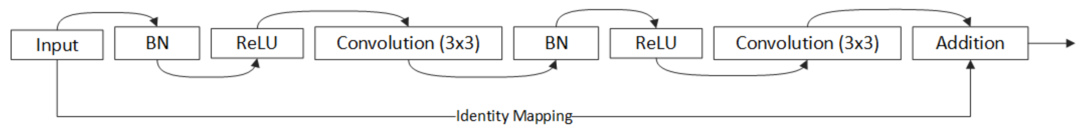
He et al. proposed the Residual neural Network (ResNet) to facilitate training and address degradation problems such as vanishing gradients in deep networks [46]. Each residual unit can be illustrated as a general form
where , are the input and output of the residual unit, is the residual function, is the activation function and is an identity mapping function. In ResNet, multiple combinations of Batch Normalization (BN), ReLU activation, and convolutional layers exist. ResU-Net combines the strengths of both deep residual learning and the U-Net architecture [44] to improve performance over the default U-Net architecture [46]. Figure 2 shows the residual unit with identity mapping used in ResU-Net.
Similar to U-Net, ResU-Net comprises three parts: encoding, bridge, and decoding. The first part encodes the input image into compact representations. The second part serves as a bridge connecting the encoding and decoding paths. The last part recovers the representations to obtain a pixel-wise categorization, e.g., semantic segmentation. After the last level of the decoding phase (in both U-Net and ResU-Net architecture), a 1 × 1 convolution and a sigmoid activation layer is used to project the multi-channel feature maps into the desired segmentation [46].
2.3. Study Area and Dataset
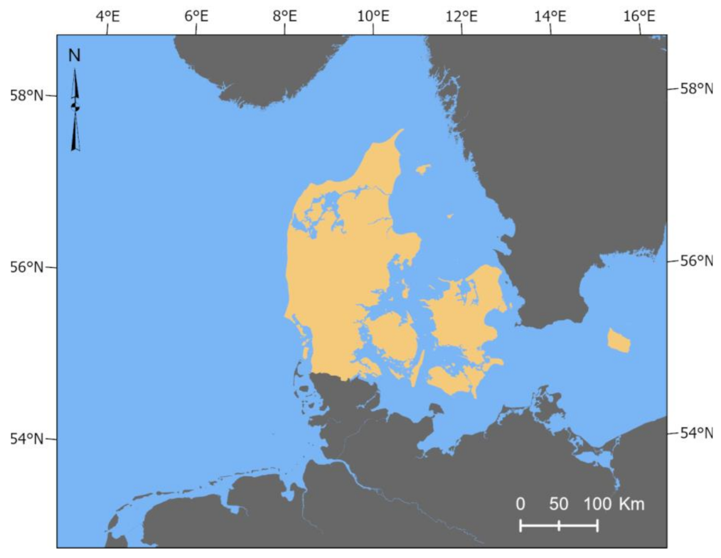
The proposed method is trained and verified on a dataset covering the entire landmass of Denmark (Figure 3). Denmark is a country in Northern Europe, bordering Germany to the south. It is part of the so-called Nordic countries (incl. Sweden, Norway, Finland, and Iceland). Denmark has a total land area of 42,937.80 km2, of which an estimated 60% is cultivated [47] (21% more than the average for the European Union in 2016) [48]. For Denmark, this proportion has remained stable for at least 10 years according to Eurostat statistics [48,49]. In 2018, about half of the cultivated area was used for the production of cereals, primarily winter wheat and spring barley [50]. According to the “Precision agriculture 2018” publication by Statistics Denmark, about 32% of farms have been involved in continuing education programs during 2018. More than 23% of the farms of the country use precision agriculture technology regularly [50]. These investments in agriculture put Denmark among the leading countries in terms of primary production efficiency worldwide.
In our study, we used free-of-charge Sentinel-2 data. The Sentinel-2 constellation consists of two satellites (A and B), launched in June 2015 and March 2017, respectively. It is part of the Copernicus program by the European Commission in collaboration with the European Space Agency. Both satellites carry the MultiSpectral Imager (MSI) instrument with 13 spectral bands in total. Compared to other missions such as Landsat, Sentinel-2 offers several improvements. First, it adds spectral bands in the red-edge region that are particularly useful for vegetation applications, as well as a water vapor absorption band. Second, the spatial resolution of bands in the visible and near-infrared region is increased to 10 and 20 m. Third, the full mission specification of the twin satellites flying in the same orbit but phased at 180°, is designed to give a high revisit frequency of 5 days at the Equator. We have used bands 2, 3, 4, 8 of Sentinel-2 L1C data at 10 m resolution. The product is top of atmosphere reflectance, orthorectified, co-registered. Sentinel-2 images were obtained for the year 2017. Training requires images with low cloud coverage for field boundaries to be identifiable. For each tile, the Sentinel-2 image with a cloud coverage percentage of less than 0.1% was used.
2.4. Network Training
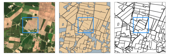
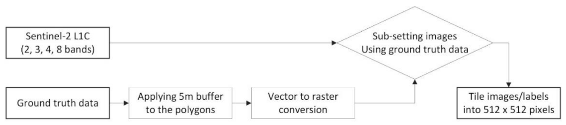
While working on training the model for field segmentation, it became clear that a field boundary/non-field boundary classification using the proposed model generates poor accuracy. A classifier of this type was not able to classify boundaries between adjacent fields at the resolution of Sentinel-2. To solve this, we instead treated the ground truth as three different classes: background (e.g., urban area, forests, water bodies), field and field boundary. Field boundary polygons were produced by taking the edges of each polygon in each shapefile and applying a buffer of 5 m to obtain a boundary region that is 10 m across, the width of a Sentinel-2 pixel. An inverse buffer of 5 m was applied to the field polygons to ensure that fields and boundaries did not overlap. The final shapefiles were then rasterized to produce a classification image for use in model training (Figure 4).
Two Sentinel-2 images from July 2017 are tiled into 512 × 512 pixels (10,650 image tiles in total). Field boundary labels for model training, comprising of 100,000 field polygons, were obtained for the year 2017 by Soilessentials [51] through manual labeling, using GPS enabled smartphones and tablets. We omitted fields that were not clearly discernable in Sentinel-2 imagery, e.g., very small fields (area less than 400 m2).
We randomly selected 70% of the dataset for training, distinguishing three classes: field boundaries, agricultural fields, and all other land covers. The dataset was balanced to contain 50% boundary and 50% non-boundary samples. The Adam algorithm was employed to optimize the weights of the network in the training stage with an initial learning rate of 0.001. The training was performed using the Tensorflow platform on a PC with 16 GB DDR memory and an NVIDIA Geforce GTX 1080 GPU with 11 GB of memory running Ubuntu 16.04.
We have followed the same procedure for selecting hyperparameters for both U-Net and ResU-Net models; Hyperparameters of the models were obtained as follows:
- A set of 10 neural networks is randomly generated from a set of allowed hyperparameters (Unit level, conv layer, input size, and filter size for each layer);
- Each network is trained for 1000 epochs and its performance on the validation set is evaluated. We have chosen this large number of epochs to ensure that each network achieves the best possible performance, and save the best performing set of weights for each network to prevent overfitting;
- The worst-performing networks are discarded, while the better-performing ones are paired up as "parents". "child" networks are then created, which randomly inherit hyperparameter values to form the next generation of networks, while the worst-performing values "die out";
- There is also a small probability for random mutations in the child networks - hyperparameter values have a small chance of randomly changing;
- This process is repeated for 10 generations, leaving only the best performing network architectures;
2.5. Accuracy Assessment
There are metrics in the literature for formally assessing a segmentation result based on reference segments, in this case, hand-delineated fields. Examples include similarity metrics quantifying the average distance between reference and predicted boundaries, or the difference in area between reference and predicted segments. Locational accuracy is certainly useful for assessing the most important aspect for the application of field boundary detection. Therefore, we assess the quality of our field boundaries model using the F1 score and Jaccard Index.
The F1 score is the harmonic mean of the precision and recall, where a score of 1 represents an optimal result (perfect precision and recall). The F1 score gives a good overview of the difference in area between the reference and trial segments. The mathematical representation of the F1 score is written as
where TP is the number of true positives, FP is the number of false positives, FN is the number of false negatives. The Jaccard Index (also known as the Jaccard coefficient) is a statistic used in understanding the similarities between sample sets. The mathematical representation of the index is written as
If A and B are both empty, Jac(A, B) = 1. We compare results with the U-Net model presented in Persello et al., 2019 which achieves state-of-the-art performance in field boundary detection [40].
3. Experimental Results
The F1 Score and Jaccard coefficient of the generated models are reported in Table 1. With an average F1 score of 0.90 and average Jaccard coefficient of 0.80 results of the ResU-Net model are better than those of the U-Net model (average F1 score of 0.88 and average Jaccard coefficient of 0.77) and are the best among all other methods (e.g., SegNet model presented in Persello et al., 2019 with an F1 score of 0.7) presented in the field boundary detection field.
4. Discussion
From the comparisons in the experimental results section, it is shown that ResU-Net can obtain comparable performance with other methods and has a better ability to model generalization. Moreover, ResU-Net is easy to train and takes less time than other models in the literature. This approach led us to the network architecture outlined in Table 2 for both U-Net and ReU-Net, which was trained using the Adam optimization algorithm.
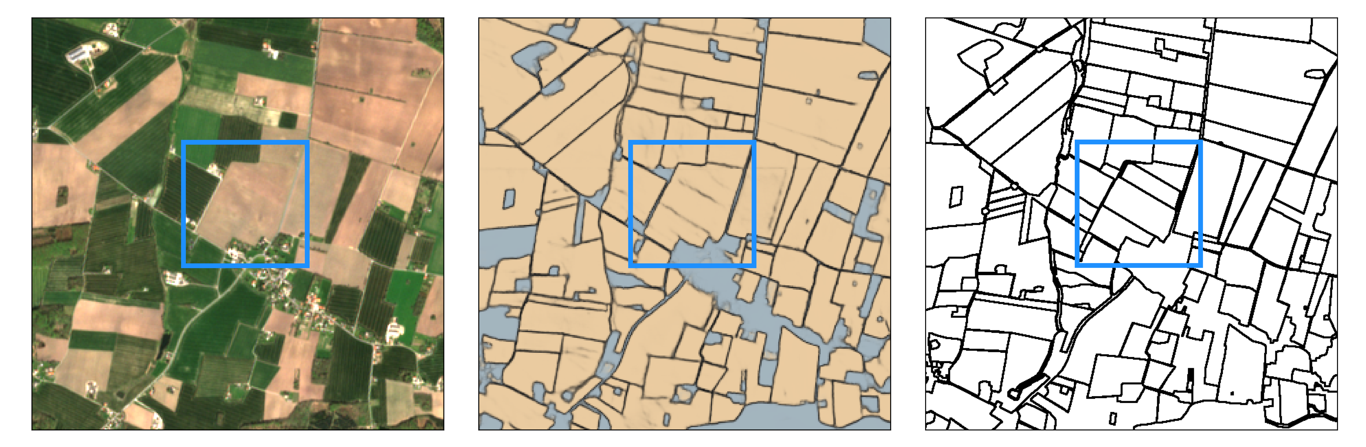
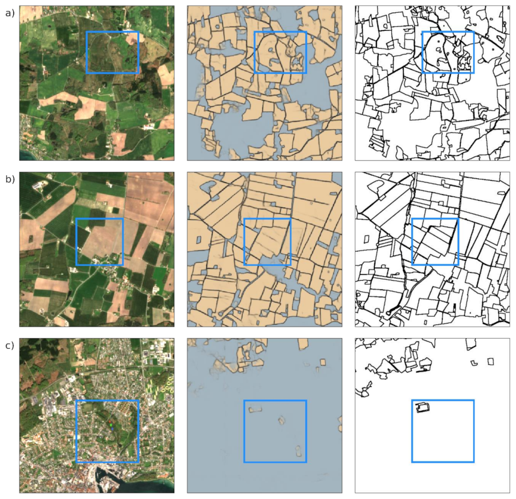
In general, the interpretation of some boundaries is ambiguous. In the first example in Figure 5a, it is difficult to decide if the structures visible in the highlighted area are actual field boundaries or only anomalies within otherwise coherent fields. In this case, the model detected some but not all the structures highlighted in the reference data. Such ambiguity may also vary with the timing of the input image used for prediction in case the structures are only temporarily visible.
This example also demonstrates that even non-agricultural areas with similar characteristics to some croplands (e.g., different types of forests) have been segmented successfully. Context information is very important when analyzing objects with complex structures. Our network considers context information of field boundaries, thus can distinguish field boundaries from similar objects such as agricultural croplands, forests, or grasslands.
Issues, however, arise from field patterns and only weakly visible boundaries. In the (b) example in Figure 5b, the model result indicates the highlighted area would probably be interpreted as one large field while the reference data suggests it being multiple separate fields. When looking at the original image, this separation is only vaguely visible. In this case, the available image may not be the most appropriate one for distinguishing these fields as they are clearly all fallows and barely distinguishable at this time of the year. Imagery from different stages of the growing season may reveal a clearer pattern. These types of boundaries, however, pose a challenge during data labeling as well since they are often not even clearly distinguishable for a human interpreter.
The objects highlighted in the (c) example in Figure 5c again show the difficulty of interpretation date. These areas may actually be fields or meadows or, more likely given their vicinity to an urban area, greenspaces like parks (further supported by the reference data). The model correctly detected the whole surrounding area as non-agricultural but apparently considered some patches as farmland due to their similarity to fully grown crops and meadows. Possibly, a distinction of different types of non-agricultural areas would help prevent this.
It is shown that the ResU-Net model produces less noisy but more completely changed regions (e.g., the whole fields) and better inner regional consistency. U-Net can get a clearer boundary of the fields than ResU-Net. Smaller fields were occasionally missed or merged into larger fields in U-Net. This can be explained in part by issues in inconsistent boundaries or some falsely detected boundaries within the fields. However, in the ResU-Net model, smaller fields are not missed and detected in detail. Both models (ResU-Net and U-Net) are less susceptible to noise and the background and get clearer changed regions (e.g., the whole fields) compared to other models in the literature [40,41,42].
5. Conclusions
In this paper, we proposed a field boundary detection model based on the deep fully convolutional network architecture called ResU-Net to produce a segmentation delineating agricultural fields. The experimental analysis conducted using Sentinel-2 imagery of Denmark shows promising results. The proposed model compares favorably against state-of-the-art U-Net models in terms of the accuracy in terms of F1 score and Jaccard coefficient metrics. A visual inspection of the obtained segmentation results showed accurate field boundaries that are close to human photo-interpretation. These results demonstrate that the proposed model could facilitate fast and accurate boundary extraction be that may be incorporated into an object-based cropland analysis service. Other aspects that need to be further investigated are the use of multi-temporal data and the fusion of panchromatic and multispectral bands within a multiscale field boundary detection scheme.
Author Contributions
Conceptualization, methodology, and validation were carried out by A.T.; original draft preparation by A.T. and M.P.W.; review and editing were carried out by A.T., M.P.W., D.P. and R.B. All authors have read and agreed to the published version of the manuscript.
Funding
This study is a part of the BETTER project funded by EC-H2020 (grant no. 776280).
Data Availability
The satellite data used in this study are openly available in Copernicus Open Access Hub at https://scihub.copernicus.eu (accessed on 21 January 2021).
Acknowledgments
The authors appreciate the support by Soilessentials, providing ground truth data. We would like to thank Matt Grayling for helping us improving our U-Net model.
Conflicts of Interest
The authors declare no conflict of interest.
References
- Debats, S.R.; Luo, D.; Estes, L.D.; Fuchs, T.J.; Caylor, K.K. A generalized computer vision approach to mapping crop fields in heterogeneous agricultural landscapes. Remote Sens. Environ. 2016, 179, 210–221. [Google Scholar] [CrossRef] [Green Version]
- Belgiu, M.; Csillik, O. Sentinel-2 cropland mapping using pixel-based and object-based time-weighted dynamic time warping analysis. Remote Sens. Environ. Remote Sens. Environ. 2018, 204, 509–523. [Google Scholar] [CrossRef]
- Garcia-Pedrero, A.; Gonzalo-Martín, C.; Lillo-Saavedra, M.; Rodríguez-Esparragón, D. The Outlining of Agricultural Plots Based on Spatiotemporal Consensus Segmentation. Remote Sens. 2018, 10, 1991. [Google Scholar] [CrossRef] [Green Version]
- Turker, M.; Kok, E.H. Field-based sub-boundary extraction from remote sensing imagery using perceptual grouping. ISPRS J. Photogramm. Remote Sens. 2013, 79, 106–121. [Google Scholar] [CrossRef]
- Shawon, A.R.; Ko, J.; Ha, B.; Jeong, S.; Kim, D.K.; Kim, H.-Y. Assessment of a Proximal Sensing-integrated Crop Model for Simulation of Soybean Growth and Yield. Remote Sens. 2020, 12, 410. [Google Scholar] [CrossRef] [Green Version]
- Yan, L.; Roy, D.P. Automated crop field extraction from multi-temporal Web Enabled Landsat Data. Remote Sens. Environ. 2014, 144, 42–64. [Google Scholar] [CrossRef] [Green Version]
- Yan, L.; Roy, D.P. Conterminous United States crop field size quantification from multi-temporal Landsat data. Remote Sens. Environ. 2016, 172, 67–86. [Google Scholar] [CrossRef] [Green Version]
- Canny, J. A Computational Approach to Edge Detection. IEEE Trans. Pattern Anal. Mach. Intell. 1986, PAMI-8, 679–698. [Google Scholar] [CrossRef]
- Nevatia, R.; Babu, K.R. Linear feature extraction and description. Comput. Graphics Image Proc. 1980, 13, 257–269. [Google Scholar] [CrossRef]
- Wagner, M.P.; Oppelt, N. Extracting Agricultural Fields from Remote Sensing Imagery Using Graph-Based Growing Contours. Remote Sens. 2020, 12, 1205. [Google Scholar] [CrossRef] [Green Version]
- Kettig, R.L.; Landgrebe, D.A. Classification of multispectral image data by extraction and classification of homogeneous objects. IEEE Trans. Geosci. Electron. 1976, 14, 19–26. [Google Scholar] [CrossRef] [Green Version]
- Pal, S.K.; Mitra, P. Multispectral image segmentation using the rough-set-initialized EM algorithm. IEEE Trans. Geosci. Remote Sens. 2002, 40, 2495–2501. [Google Scholar] [CrossRef] [Green Version]
- Robertson, T.V. Extraction and classification of objects in multispectral images. Available online: https://docs.lib.purdue.edu/cgi/viewcontent.cgi?article=1117&context=larstech (accessed on 15 February 2021).
- Theiler, J.P.; Gisler, G. Contiguity-Enhanced k-means Clustering Algorithm for Unsupervised Multispectral Image Segmentation. In Proceedings of the Algorithms, Devices, and Systems for Optical Information Processing. Available online: https://public.lanl.gov/jt/Papers/cluster-spie.pdf (accessed on 15 February 2021).
- Bertasius, G.; Shi, J.; Torresani, L. DeepEdge: A multi-scale bifurcated deep network for top-down contour detection. In Proceedings of the 2015 IEEE Conference on Computer Vision and Pattern Recognition (CVPR), Santiago, Chile, 7–12 June 2015; pp. 4380–4389. [Google Scholar]
- Maninis, K.-K.; Pont-Tuset, J.; Arbelaez, P.; Van Gool, L. Convolutional Oriented Boundaries: From Image Segmentation to High-Level Tasks. IEEE Trans. Pattern Anal. Mach. Intell. 2018, 40, 819–833. [Google Scholar] [CrossRef] [PubMed] [Green Version]
- Wei, S.; Xinggang, W.; Yan, W.; Xiang, B.; Zhang, Z. DeepContour: A deep convolutional feature learned by positive-sharing loss for contour detection. In Proceedings of the 2015 IEEE Conference on Computer Vision and Pattern Recognition (CVPR), Santiago, Chile, 7–12 June 2015; pp. 3982–3991. [Google Scholar]
- Xie, S.; Tu, Z. Holistically-Nested Edge Detection. In Proceedings of the 2015 IEEE International Conference on Computer Vision (ICCV), Santiago, Chile, 7–13 December 2015; pp. 1395–1403. [Google Scholar]
- Krizhevsky, A.; Sutskever, I.; Hinton, G.E. Imagenet classification with deep convolutional neural networks. Commun. ACM 2017, 60, 84–90. [Google Scholar] [CrossRef]
- Rawat, W.; Wang, Z. Deep Convolutional Neural Networks for Image Classification: A Comprehensive Review. Neural Comput. 2017, 29, 2352–2449. [Google Scholar] [CrossRef] [PubMed]
- Simonyan, K.; Zisserman, A. Very deep convolutional networks for large-scale image recognition. arXiv 2014, arXiv:1409.1556. [Google Scholar]
- Szegedy, C.; Liu, W.; Jia, Y.; Sermanet, P.; Reed, S.; Anguelov, D.; Erhan, D.; Vanhoucke, V.; Rabinovich, A. Going deeper with convolutions. In Proceedings of the IEEE Conference on Computer Vision and Pattern Recognition, Boston, MA, USA, 21 June 2015; pp. 1–9. [Google Scholar]
- Cheng, G.; Yang, C.; Yao, X.; Guo, L.; Han, J. When Deep Learning Meets Metric Learning: Remote Sensing Image Scene Classification via Learning Discriminative CNNs. IEEE Trans. Geosci. Remote Sens. 2018, 56, 2811–2821. [Google Scholar] [CrossRef]
- Bergado, J.R.; Persello, C.; Gevaert, C. A deep learning approach to the classification of sub-decimetre resolution aerial images. In Proceedings of the 2016 IEEE International Geoscience and Remote Sensing Symposium (IGARSS), Beijing, China, 10–15 July 2016; pp. 1516–1519. [Google Scholar]
- Bergado, J.R.; Persello, C.; Stein, A. Recurrent Multiresolution Convolutional Networks for VHR Image Classification. IEEE Trans. Geosci. Remote Sens. 2018, 56, 6361–6374. [Google Scholar] [CrossRef] [Green Version]
- Fu, G.; Liu, C.; Zhou, R.; Sun, T.; Zhang, Q. Classification for High Resolution Remote Sensing Imagery Using a Fully Convolutional Network. Remote Sens. 2017, 9, 498. [Google Scholar]
- Maggiori, E.; Tarabalka, Y.; Charpiat, G.; Alliez, P. Convolutional Neural Networks for Large-Scale Remote-Sensing Image Classification. IEEE Trans. Geosci. Remote Sens. 2017, 55, 645–657. [Google Scholar] [CrossRef] [Green Version]
- Paisitkriangkrai, S.; Sherrah, J.; Janney, P.; Van Den Hengel, A. Semantic labeling of aerial and satellite imagery. IEEE J. Sel. Top. Appl. Earth Obs. Remote Sens. 2016, 9, 2868–2881. [Google Scholar] [CrossRef]
- Volpi, M.; Tuia, D. Dense Semantic Labeling of Subdecimeter Resolution Images With Convolutional Neural Networks. IEEE Trans. Geosci. Remote Sens. 2017, 55, 881–893. [Google Scholar] [CrossRef] [Green Version]
- Cheng, G.; Li, Z.; Han, J.; Yao, X.; Guo, L. Exploring Hierarchical Convolutional Features for Hyperspectral Image Classification. IEEE Trans. Geosci. Remote Sens. 2018, 56, 6712–6722. [Google Scholar] [CrossRef]
- Ghamisi, P.; Chen, Y.; Zhu, X.X. A self-improving convolution neural network for the classification of hyperspectral data. IEEE Geosci. Remote Sens. Lett. 2016, 13, 1537–1541. [Google Scholar] [CrossRef] [Green Version]
- Zhao, W.; Du, S. Spectral–spatial feature extraction for hyperspectral image classification: A dimension reduction and deep learning approach. IEEE Trans. Geosci. Remote Sens. 2016, 54, 4544–4554. [Google Scholar] [CrossRef]
- Chen, S.; Wang, H.; Xu, F.; Jin, Y.-Q. Target Classification Using the Deep Convolutional Networks for SAR Images. IEEE Trans. Geosci. Remote Sens. 2016, 54, 4806–4817. [Google Scholar] [CrossRef]
- Long, Y.; Gong, Y.; Xiao, Z.; Liu, Q. Accurate Object Localization in Remote Sensing Images Based on Convolutional Neural Networks. IEEE Trans. Geosci. Remote Sens. 2017, 55, 2486–2498. [Google Scholar] [CrossRef]
- Gevaert, C.M.; Persello, C.; Nex, F.; Vosselman, G. A deep learning approach to DTM extraction from imagery using rule-based training labels. ISPRS J. Photogramm. Remote Sens. 2018, 142, 106–123. [Google Scholar] [CrossRef]
- Rizaldy, A.; Persello, C.; Gevaert, C.; Oude Elberink, S.J. Fully convolutional networks for ground classification from lidar point clouds. Remote Sens. Spat. Inf. Sci. 2018, 4. [Google Scholar] [CrossRef] [Green Version]
- Mboga, N.; Persello, C.; Bergado, J.R.; Stein, A. Detection of Informal Settlements from VHR Images Using Convolutional Neural Networks. Remote Sens. 2017, 9, 1106. [Google Scholar] [CrossRef] [Green Version]
- Persello, C.; Stein, A. Deep Fully Convolutional Networks for the Detection of Informal Settlements in VHR Images. IEEE Geosci. Remote Sens. Lett. 2017, 14, 2325–2329. [Google Scholar] [CrossRef]
- Taravat, A.; Grayling, M.; Talon, P.; Petit, D. Boundary delineation of agricultural fields using convolutional NNs. In Proceedings of the ESA Phi Week, Rome, Italy, 9–13 September 2019. [Google Scholar]
- Persello, C.; Tolpekin, V.A.; Bergado, J.R.; de By, R.A. Delineation of agricultural fields in smallholder farms from satellite images using fully convolutional networks and combinatorial grouping. Remote Sens. Environ. 2019, 231, 111253. [Google Scholar] [CrossRef] [PubMed]
- Xia, X.; Persello, C.; Koeva, M. Deep Fully Convolutional Networks for Cadastral Boundary Detection from UAV Images. Remote Sens. 2019, 11, 1725. [Google Scholar] [CrossRef] [Green Version]
- Masoud, K.M.; Persello, C.; Tolpekin, V.A. Delineation of Agricultural Field Boundaries from Sentinel-2 Images Using a Novel Super-Resolution Contour Detector Based on Fully Convolutional Networks. Remote Sens. 2020, 12, 59. [Google Scholar] [CrossRef] [Green Version]
- Zhang, Z.; Liu, Q.; Wang, Y. Road Extraction by Deep Residual U-Net. IEEE Geosci. Remote Sens. Lett. 2018, 15, 749–753. [Google Scholar] [CrossRef] [Green Version]
- Ronneberger, O.; Fischer, P.; Brox, T. U-net: Convolutional networks for biomedical image segmentation. In Proceedings of the International Conference on Medical Image Computing and Computer-Assisted Intervention, Munich, Germany, 5 October 2015; pp. 234–241. [Google Scholar]
- Long, J.; Shelhamer, E.; Darrell, T. Fully convolutional networks for semantic segmentation. In Proceedings of the IEEE Conference on Computer Vision and Pattern Recognition, Boston, MA, USA, 7–12 June 2015; pp. 3431–3440. [Google Scholar]
- He, K.; Zhang, X.; Ren, S.; Sun, J. Deep residual learning for image recognition. In Proceedings of the IEEE Conference on Computer Vision and Pattern Recognition, Las Vegas, NV, USA, 30 June 2016; pp. 770–778. [Google Scholar]
- Statistics Denmark: Area. Available online: https://www.dst.dk/en/Statistik/emner/geografi-miljoe-og-energi/areal/areal (accessed on 15 February 2021).
- Eurostat: Agriculture, Forestry and Fishery Statistics. Available online: https://ec.europa.eu/eurostat/statistics-explained/index.php?title=Agriculture,_forestry_and_fishery_statistics (accessed on 15 February 2021).
- Eurostat: Utilized Agricultural Area by Categories. Available online: https://ec.europa.eu/eurostat/databrowser/view/tag00025/default/table?lang=en (accessed on 15 February 2021).
- Statistics Denmark: Agriculture, Horticulture and Forestry. Available online: https://www.dst.dk/en/Statistik/emner/erhvervslivets-sektorer/landbrug-gartneri-og-skovbrug (accessed on 15 February 2021).
- SoilEssentials. Available online: https://www.soilessentials.com (accessed on 15 February 2021).
Figure 1.
Plain neural unit used in U-Net.

Figure 2.
Residual unit with identity mapping used in the ResU-Net.

Figure 3.
Denmark as the study area.

Figure 4.
A schematic view of the ground truth data preprocessing phase.

Figure 5.
The left column represents the original image, the middle column the ground truth data, and the right column the proposed model results. Rows represent different subsets. (a) difficult to decide if the structures visible in the highlighted area are actual field boundaries or only anomalies within otherwise coherent fields. (b) the model result indicates the highlighted area would probably be interpreted as one large field while the reference data suggests it being multiple separate fields (c) the difficulty of interpretation date.


Table 1.
F1 Score and Jaccard coefficient comparisons of the generated models. Best performance highlighted in bold.
Table 1.
F1 Score and Jaccard coefficient comparisons of the generated models. Best performance highlighted in bold.
| Model Name (Unit Level, Conv Layer, Input Size) | F1 Score | Jaccard Coefficient |
|---|---|---|
| ResU-Net (8, 15, 256 × 256) | 0.87 | 0.74 |
| ResU-Net (10, 19, 512 × 512) | 0.94 | 0.87 |
| ResU-Net (12, 23, 1024 × 1024) | 0.91 | 0.79 |
| U-Net (8, 15, 256 × 256) | 0.89 | 0.76 |
| U-Net (10, 19, 512 × 512) | 0.92 | 0.83 |
| U-Net (12, 23, 1024 × 1024) | 0.83 | 0.72 |
Table 2.
The best network structure of U-Net and ResU-Net.
| Input | Unit Level | Conv Layer | Stride | Output Size |
|---|---|---|---|---|
| 512 × 512 × 4 | ||||
| Encoding | Level 1 | Conv 1 | 1 | 512 × 512 × 16 |
| Conv 2 | 1 | 512 × 512 × 16 | ||
| Level 2 | Conv 3 | 2 | 256 × 256 × 32 | |
| Conv 4 | 1 | 256 × 256 × 32 | ||
| Level 3 | Conv 5 | 2 | 128 × 128 × 64 | |
| Conv 6 | 1 | 128 × 128 × 64 | ||
| Level 4 | Conv 7 | 2 | 64 × 64 × 128 | |
| Conv 8 | 1 | 64 × 64 × 128 | ||
| Bridge | Level 5 | Conv 9 | 2 | 32 × 32 × 256 |
| Conv 10 | 1 | 32 × 32 × 256 | ||
| Decoding | Level 6 | Conv 11 | 1 | 64 × 64 × 128 |
| Conv 12 | 1 | 64 × 64 × 128 | ||
| Level 7 | Conv 13 | 1 | 128 × 128 × 64 | |
| Conv 14 | 1 | 128 × 128 × 64 | ||
| Level 8 | Conv 15 | 1 | 256 × 256 × 32 | |
| Conv 16 | 1 | 256 × 256 × 32 | ||
| Level 9 | Conv 17 | 1 | 512 × 512 × 16 | |
| Conv 18 | 1 | 512 × 512 × 16 | ||
| Output | Level 10 | Conv 19 | 1 | 512 × 512 × 3 |
Publisher’s Note: MDPI stays neutral with regard to jurisdictional claims in published maps and institutional affiliations. |
© 2021 by the authors. Licensee MDPI, Basel, Switzerland. This article is an open access article distributed under the terms and conditions of the Creative Commons Attribution (CC BY) license (http://creativecommons.org/licenses/by/4.0/).
Share and Cite
MDPI and ACS Style
Taravat, A.; Wagner, M.P.; Bonifacio, R.; Petit, D. Advanced Fully Convolutional Networks for Agricultural Field Boundary Detection. Remote Sens. 2021, 13, 722. https://0-doi-org.brum.beds.ac.uk/10.3390/rs13040722
AMA Style
Taravat A, Wagner MP, Bonifacio R, Petit D. Advanced Fully Convolutional Networks for Agricultural Field Boundary Detection. Remote Sensing. 2021; 13(4):722. https://0-doi-org.brum.beds.ac.uk/10.3390/rs13040722
Chicago/Turabian StyleTaravat, Alireza, Matthias P. Wagner, Rogerio Bonifacio, and David Petit. 2021. "Advanced Fully Convolutional Networks for Agricultural Field Boundary Detection" Remote Sensing 13, no. 4: 722. https://0-doi-org.brum.beds.ac.uk/10.3390/rs13040722
Note that from the first issue of 2016, this journal uses article numbers instead of page numbers. See further details here.