
Deep Learning of Sea Surface Temperature Patterns to Identify Ocean Extremes


1
Affiliate of the Department of Ocean Sciences, University of California, Santa Cruz, CA 95064, USA
2
Department of Astronomy and Astrophysics, University of California, Santa Cruz, CA 95064, USA
3
Kavli Institute for the Physics and Mathematics of the Universe (Kavli IPMU), 5-1-5 Kashiwanoha, Kashiwa 277-8583, Japan
4
Graduate School of Oceanography, University of Rhode Island, Narragansett, RI 02882, USA
5
Department of Physics, University of California, Santa Cruz, CA 95064, USA
*
Author to whom correspondence should be addressed.
†
Current address: 1156 High St., University of California, Santa Cruz, CA 95064, USA.
‡
These authors contributed equally to this work.
Remote Sens. 2021, 13(4), 744; https://0-doi-org.brum.beds.ac.uk/10.3390/rs13040744
Submission received: 24 January 2021
/
Revised: 10 February 2021
/
Accepted: 12 February 2021
/
Published: 17 February 2021
Abstract
:We performed an out-of-distribution (OOD) analysis of ∼12,000,000 semi-independent 128 × 128 pixel sea surface temperature (SST) regions, which we define as cutouts, from all nighttime granules in the MODIS R2019 Level-2 public dataset to discover the most complex or extreme phenomena at the ocean’s surface. Our algorithm (ULMO) is a probabilistic autoencoder (PAE), which combines two deep learning modules: (1) an autoencoder, trained on ∼150,000 random cutouts from 2010, to represent any input cutout with a 512-dimensional latent vector akin to a (non-linear) Empirical Orthogonal Function (EOF) analysis; and (2) a normalizing flow, which maps the autoencoder’s latent space distribution onto an isotropic Gaussian manifold. From the latter, we calculated a log-likelihood (LL) value for each cutout and defined outlier cutouts to be those in the lowest 0.1% of the distribution. These exhibit large gradients and patterns characteristic of a highly dynamic ocean surface, and many are located within larger complexes whose unique dynamics warrant future analysis. Without guidance, ULMO consistently locates the outliers where the major western boundary currents separate from the continental margin. Prompted by these results, we began the process of exploring the fundamental patterns learned by ULMO thereby identifying several compelling examples. Future work may find that algorithms such as ULMO hold significant potential/promise to learn and derive other, not-yet-identified behaviors in the ocean from the many archives of satellite-derived SST fields. We see no impediment to applying them to other large remote-sensing datasets for ocean science (e.g., SSH and ocean color).
1. Introduction
Satellite-borne sensors have for many years been collecting data used to estimate a broad range of meteorological, oceanographic, terrestrial and cryospheric properties. Of significance with regard to the fields associated with these properties is their global coverage and relatively high spatial (meters to tens of kilometers) and temporal (hours to tens of days) resolutions. These datasets tend to be very large, well documented and readily accessible, making them ideal targets for analyses using modern machine learning techniques. Based on our knowledge of, interest in and access to global sea surface temperature (SST) datasets, we have chosen one of these to explore the possibilities. Specifically, inspired by the question of “what lurks within” and also the desire to identify complex and/or extreme phenomena of the upper ocean, we have developed an unsupervised machine learning algorithm named ULMO [1] to analyze the nighttime MODerate-resolution Imaging Spectroradiometer (MODIS) Level-2 (L2) [2] seat surface temperature (SST) dataset obtained from the NASA spacecraft Aqua, spanning years 2003–2019. The former (the unknown unknowns) could reveal previously unanticipated physical processes at or near the ocean’s surface. Such surprises are, by definition, rare and require massive datasets and semi-automated approaches to examine them. The latter type (extrema) affords an exploration of the incidence and spatial distribution of complex phenomena across the entire ocean. Similar “fishing” expeditions have been performed in other fields on large imaging datasets (e.g., astronomy [3]). However, to our knowledge, this is the first application of machine learning for open-ended exploration of a large oceanographic dataset, although there is a rapidly growing body of literature on applying machine learning techniques to the specifics of SST retrieval algorithms [4], cloud detection [5], eddy location [6], prediction [7,8,9], etc., and more generally, to remote sensing [10].
Previous analyses of SST on local or global scales have emphasized standard statistics (e.g., mean and RMS) and/or linear methods for pattern assessment (e.g., FFT and EOF). While these metrics and techniques offer fundamental measures of the SST fields, they may not fully capture the complexity inherent in the most dynamic regions of the ocean. Motivated by advances in the analysis of natural images in computer vision, we employ a probabilistic autoencoder (PAE) which utilizes a Convolutional Neural Network (CNN) to learn the diversity of SST patterns. By design, the CNN learns the features most salient to the dataset, with built-in methodology to examine the image on a wide range of scales. Further, its non-linearity and invariance to translation offer additional advantages over the Empirical Orthogonal Function (EOF) and like applications.
The ULMO algorithm is a PAE, a deep learning tool designed for density estimation. By combining an autoencoder with a normalizing flow, the PAE is able to approximate the likelihood function for arbitrary data while also avoiding a common downfall of flow models: their sensitivity to noisy or otherwise uninformative background features in the input [11]. By first reducing our raw data (an SST field) to a compact set of the most pertinent learned features via the non-linear compression of an autoencoder, the PAE then provides an estimate of its probability by transforming the latent vector into a sample from an equal-dimension isotropic Gaussian distribution where computing the probability is trivial. We can then select the lowest probability fields as outliers or anomalous.
The secondary goal of this manuscript is to pioneer the process for like studies on other large earth science datasets in general and oceanographic datasets in particular, including those associated with the outputs of numerical models. A similar analysis of SST fields output by ocean circulation models is of particular interest as an adjunct to the work presented herein. As will become clear, we understand some of the segmentation suggested by ULMO, but not all of it. The method has also identified some anomalous events for which the basic physics is not clear. Assuming that the analysis of model-derived SST fields yields similar results, the additional output available from the model, the vector velocity field and salinity and a time series of fields, will allow for a dynamic investigation of the processes involved.
This manuscript is organized as follows: Section 2 describes the data analyzed here, Section 3 details the methodology, Section 4 presents the primary results and Section 5 provides a brief set of conclusions. All of the software and final data products generated by this study are available online https://github.com/AI-for-Ocean-Science/ulmo (accessed on 23 February 2021).
2. Data
With a primary goal of identifying regions of the ocean exhibiting rare yet physical phenomena, we chose to focus on the L2 SST Aqua MODIS dataset (https://oceancolor.gsfc.nasa.gov/data/aqua/ accessed on 23 February 2021). The associated five minute segments, each covering ≈2000 × 1350 km of the Earth’s surface and referred to as granules, have ≈1 km spatial resolution and span the entire ocean, clouds permitting, twice daily. For this study, we examined all nighttime granules from 2003–2019. The SST fields, the primary element of these granules, were processed by the Ocean Biology Processing Group (OBPG) at NASA’s Goddard Space Flight Center, Ocean Ecology Laboratory from the MODIS radiometric data using the R2019 retrieval algorithm [12] and were uploaded from the OBPG’s public server (https://oceancolor.gsfc.nasa.gov/cgi/browse.pl?sen=amod, accessed on 23 February 2021) to the University of Rhode Island (URI).
The method developed here requires a set of same-sized images. When exploring complex physical phenomena in the ocean, one is often interested in one of two spatial scales determined by the relative importance of rotation to inertia in the associated processes. The separation between these scales is generally taken to be the Rossby radius of deformation, , which, at mid-latitude is km. Processes with scales larger than are referred to as mesoscale processes, in which the importance of rotation dominates. At smaller scales the processes are referred to as sub-mesoscale. For this study, we chose to focus on the former and extracted pixel images, which we refer to as cutouts, from the MODIS granules. Cutouts are approximately 128 km on the side. We are confident, supported by limited experimentation, that the techniques described here will apply to other scales as well.
The analysis was further restricted to data within 480 pixels of nadir. This constraint was added to reduce the influence of pixel size on the selection process for outliers; the along-scan size of pixels increases away from nadir as does the rate of this increase. To distances of ∼480 km the change in along-scan pixel size is less than a factor of two; at the edge of the swath the along-scan pixel size is approximately ∼5 times that at nadir.
The L2 MODIS product includes a quality flag—a measure of confidence of the retrieved SST—with values from 0 (best) to 4 (value not retrieved). The primary reason for assigning a poor quality to a pixel is due to cloud contamination although there are other issues that result in a poor quality rating [13]. A quality threshold of 2 was used for this study. As the incidence, sizes and shapes of clouds are highly variable (both temporally and spatially), an out-of-distribution (OOD) algorithm trained on images with some cloud contamination may become more sensitive to cloud patterns than unusual SST patterns. Indeed, our initial experiments were stymied by clouds with the majority of outlier cutouts showing unusual cloud patterns, suggesting an application of this approach to the study of clouds as well. To mitigate this effect, we further restricted the dataset to cutouts with very low cloud cover (CC), defined as the fraction of the cutout image masked for clouds or other image defects.
After experimenting with model performance for various choices of CC, we settled on a conservative limit of as a compromise between dataset size and our ability to further mitigate clouds (and other masked pixels) with an inpainting algorithm (see next section).
From each granule, we extracted a set of 128 × 128 cutouts satisfying and distance to nadir of the central pixel ≤ 480 km. To well-sample the granule while limiting the number of highly overlapping cutouts, we drew at most one cutout from a pre-defined 32 × 32 pixel grid on the granule. This procedure yielded ≈700,000 cutouts per year and 12,358,049 cutouts for the full analysis.
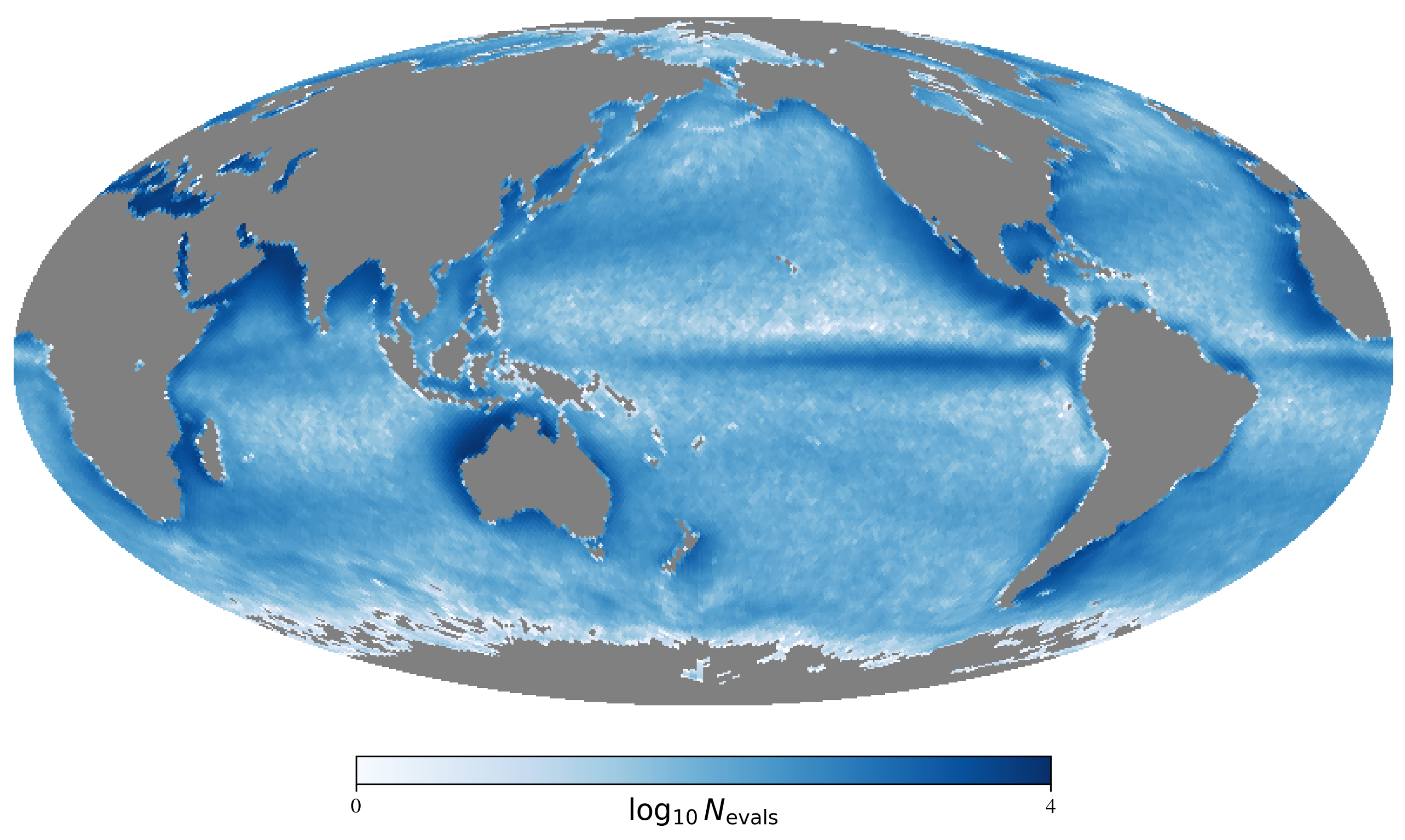
Of course, by requiring regions largely free of clouds (), we were significantly restricting the dataset and undoubtedly biasing the regions of ocean analyzed both in time and space. Figure 1 shows the spatial distribution of the full dataset across the ocean. The coastal regions show the highest incidence of multiple observations, but nearly all of the ocean was covered by one or more cutouts. Given this spatial distribution, one might naively expect the results to be biased against coastal regions because these were sampled at higher frequency and comprises a greater fraction of the full distribution. This is mitigated, in part, by the fact that the non-coastal regions cover a much larger area of the ocean, but in practice, we find that the majority of the outlier cutouts are in fact located near land.
3. Methodology
In this section, we describe the preprocessing of the SST cutouts and the architecture of our ULMO algorithm designed to discover outliers within the dataset.
3.1. Preprocessing
While modern machine learning algorithms are designed with sufficient flexibility to learn underlying patterns, gradients, etc., of images [14], standard practice is to apply initial “preprocessing” to each image to boost the performance by accentuating features of interest, or suppressing uninteresting attributes. For this project, we adopted the following pre-processing steps prior to the training and evaluation of the cutouts.
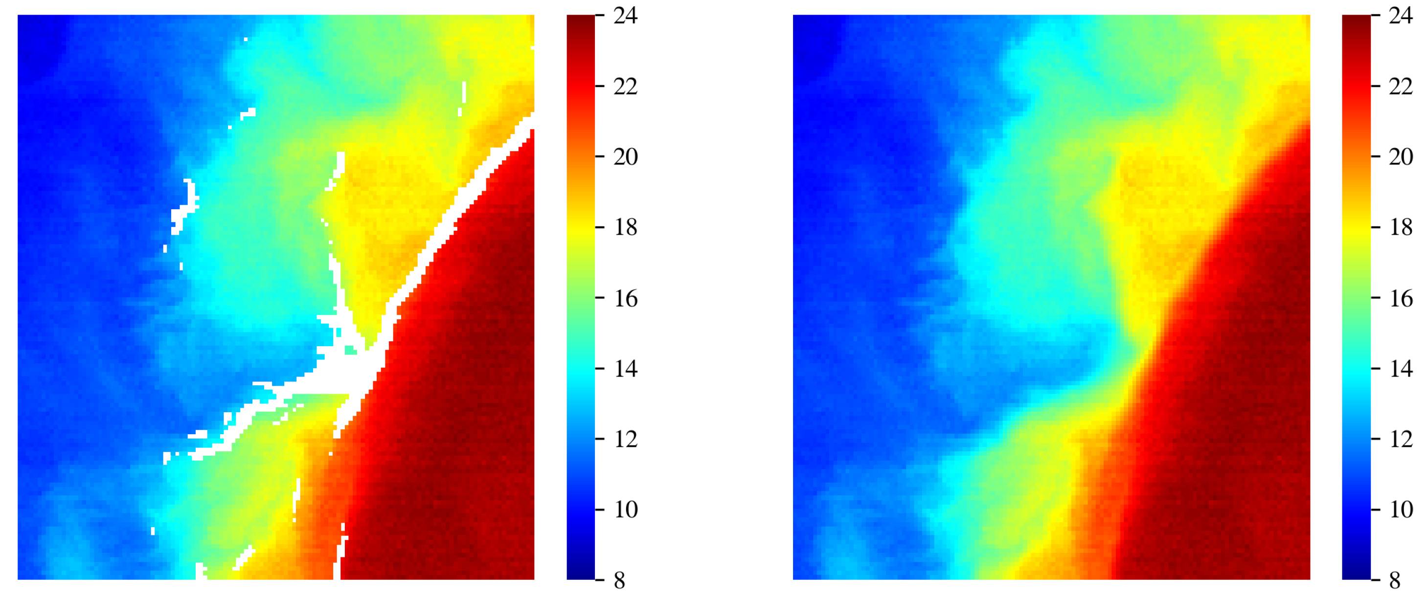
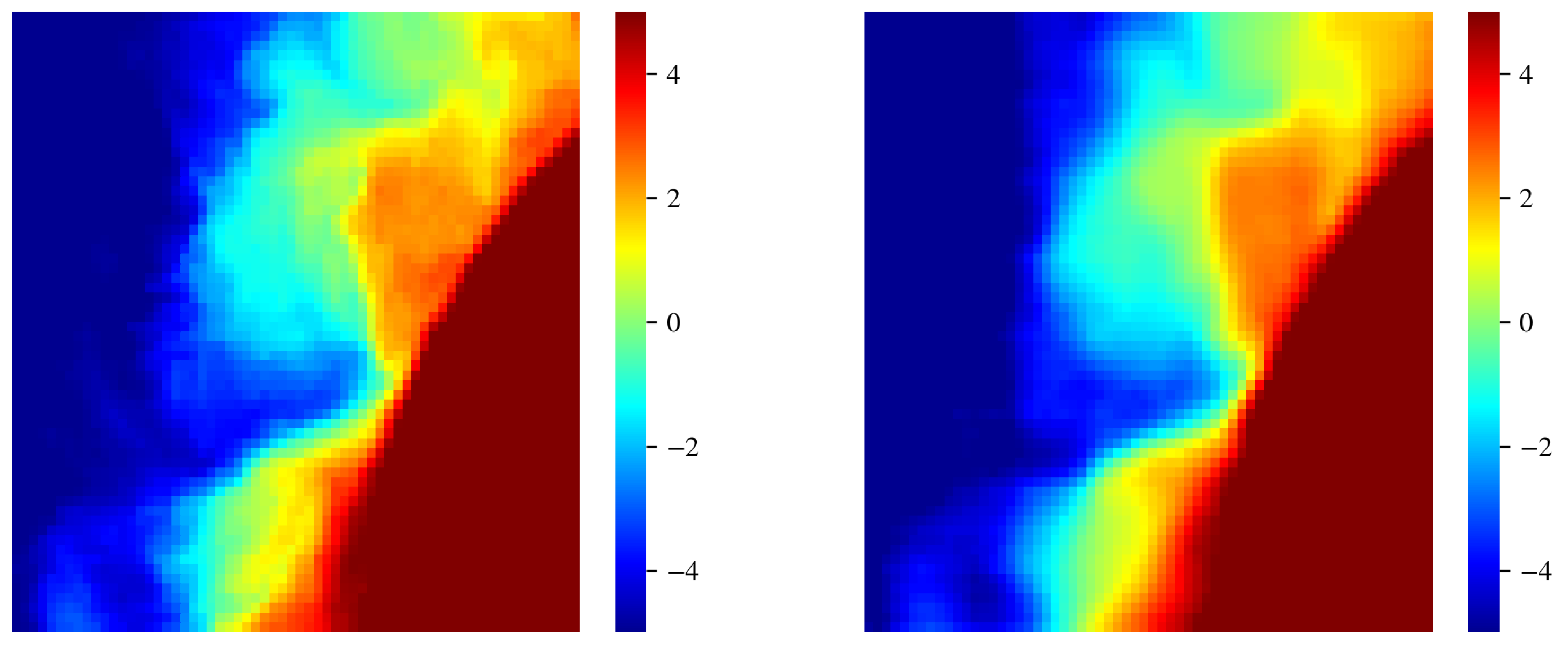
First, we mitigated the presence of clouds. As described in Section 2, this was done primarily by restricting the cutout dataset to regions with . We found, however, that even a few percent of cloud contamination can significantly affect results of the OOD algorithm. Therefore, we considered several inpainting algorithms to replace the flagged pixels with estimated values from nearby, unmasked SST values. After experimentation, we selected the Navier–Stokes method [15] based on its superior performance at preserving gradients within the cutout. Figure 2 presents an example that shows masking along a strong SST gradient (the white pixels between the red (∼22 C) and yellow (∼19 C) regions). We see that the adopted algorithm has replaced the masked data with values that preserve the sharp, underlying gradient without producing any obviously spurious patterns. As inpainting directly modifies the data, however, there is risk that the process will generate cutouts that are preferentially OOD. However, we have examined the set of outlier cutouts to find that these do not have preferentially higher CC.
Second we applied a 3 × 1 pixel median filter in the along-track direction, which reduces the presence of striping that is manifest in the MODIS L2 data product. Third, we resized the cutout to 64 × 64 pixels using the local mean, in anticipation of a future study on ocean models, which have a spatial resolution of ≈2 km [16]. Last, we subtracted the mean temperature from each cutout to focus the analysis on SST differences and avoid absolute temperature being a determining characteristic. We refer to the mean-subtracted SST values as SSTa.
3.2. Architecture
ULMO is a probabilistic autoencoder (PAE), a likelihood-based generative model which combines an autoencoder with a normalizing flow. In our model, a deep convolutional autoencoder reduces an input cutout to a latent representation with dimensions which is then transformed via the flow.
Flows [17] are invertible neural networks which map samples from a data distribution to samples from a simple base distribution, solving the density estimation problem by learning to represent complicated data as samples from a familiar distribution. The likelihood of the data can then be computed using the probability of its transformed representation under the base distribution and the determinant of the Jacobian of the transformation.
Though a flow could be applied directly to image cutouts in our use case, recent research [11] in the use of normalizing flows for OOD has revealed their sensitivity to uninformative background features which skew their estimation of the likelihood. To circumvent this issue, the PAE proposes to first reduce the input to a set of the most pertinent features via the non-linear compression of an autoencoder. The flow is then fit to the compressed representations of the image cutouts where its estimates of the likelihood are robust to the noisy or otherwise uninformative background features of the input image.
An alternative approach is the variational autoencoder (VAE) [18] which provides a lower bound on the likelihood, though empirically we found PAEs boast faster and more stable training, and are less sensitive to the user’s choice of hyperparameters.
Therefore, to summarize the advantages of our approach: (1) explicit parameterization of the likelihood function; (2) robustness of likelihood estimates to noisy and/or uninformative pixels in the input; and (3) speed and stability in training for a broad array of hyperparameter choices.
The key hyperparameters for the results that follow are presented in Table A1. Regarding , we were guided by a Principal Components Analysis (PCA) decomposition of the imaging dataset which showed that 512 components captured > 95% of the variance. The full model with 4096 input values per cutout, is comprised of parameters for the auto-encoder and parameters for the normalizing flow. It was built with PyTorch and the source code is available on GitHub—https://github.com/AI-for-Ocean-Science/ulmo (accessed on 23 February 2021).
3.3. Training
Training of the complete model consists of two, independent phases: one to develop an autoencoder that maps input cutouts into 512-dimensional latent vectors, and the other to transform the latent vectors into samples from a 512-dimensional Gaussian probability distribution function (PDF) to estimate their probability. For the autoencoder, the loss function is the standard mean squared error reconstruction loss between all pixels in the input and output cutouts. In practice, the model converged to a small loss in epochs of training.
The flow is trained by directly maximizing the likelihood of the autoencoder latent vectors. This equates to minimizing the Kullback–Leibler divergence between the data distribution and flow’s approximate distribution. Minimizing this divergence encourages the flow to fit the data distribution and thereby produce meaningful estimates of probability.
Throughout training, we used a random subset of ≈20% of the data from 2010 (135,680 cutouts). These cutouts were only used for training and are not evaluated in any of the following results.
Figure 3 shows an example of a preprocessed input SSTa cutout and the resultant reconstruction cutout from the autoencoder. As designed, the output is a good reconstruction albeit at a lower resolution that does not capture all of the finer features due to the information bottleneck in the autoencoder’s latent space but it does capture the mesoscale structure of the field. For the normalizing flow, we used a cutout batch size of 64 and a learning rate of 0.00025. Similarly, we found ≈10 epochs were sufficient to achieve convergence.
We performed training on the Nautilus distributed computing system with a single GPU. In this training setup, a single epoch for the auto-encoder requires 100 s while a single epoch for the flow requires ≈900 s.
4. Results and Discussion
In this section, we report on the main results of our analysis with primary emphasis on outlier detection. We also begin an exploration of the ULMO model to better understand the implications of deep learning for analyzing remote-sensing imaging; these will be expanded upon in future works.
4.1. The Outlier Cutouts Sample
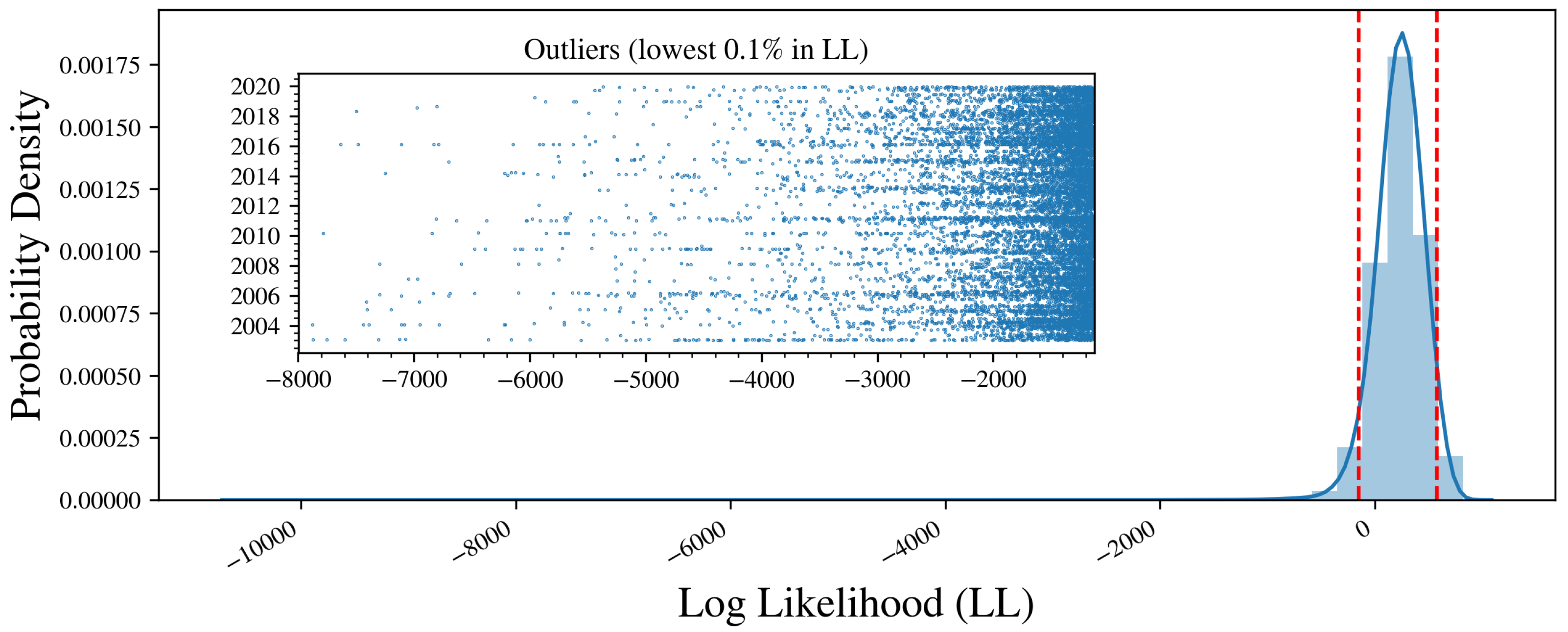
Figure 4 shows the LL distribution for all extracted cutouts modulo the set of training cutouts from 2010. The distribution peaks at LL ≈ 240 with a tail to very low values. The latter is presented in the inset which shows the lowest 0.1% of the distribution; these define the outlier cutouts of the full sample (or outliers for short).
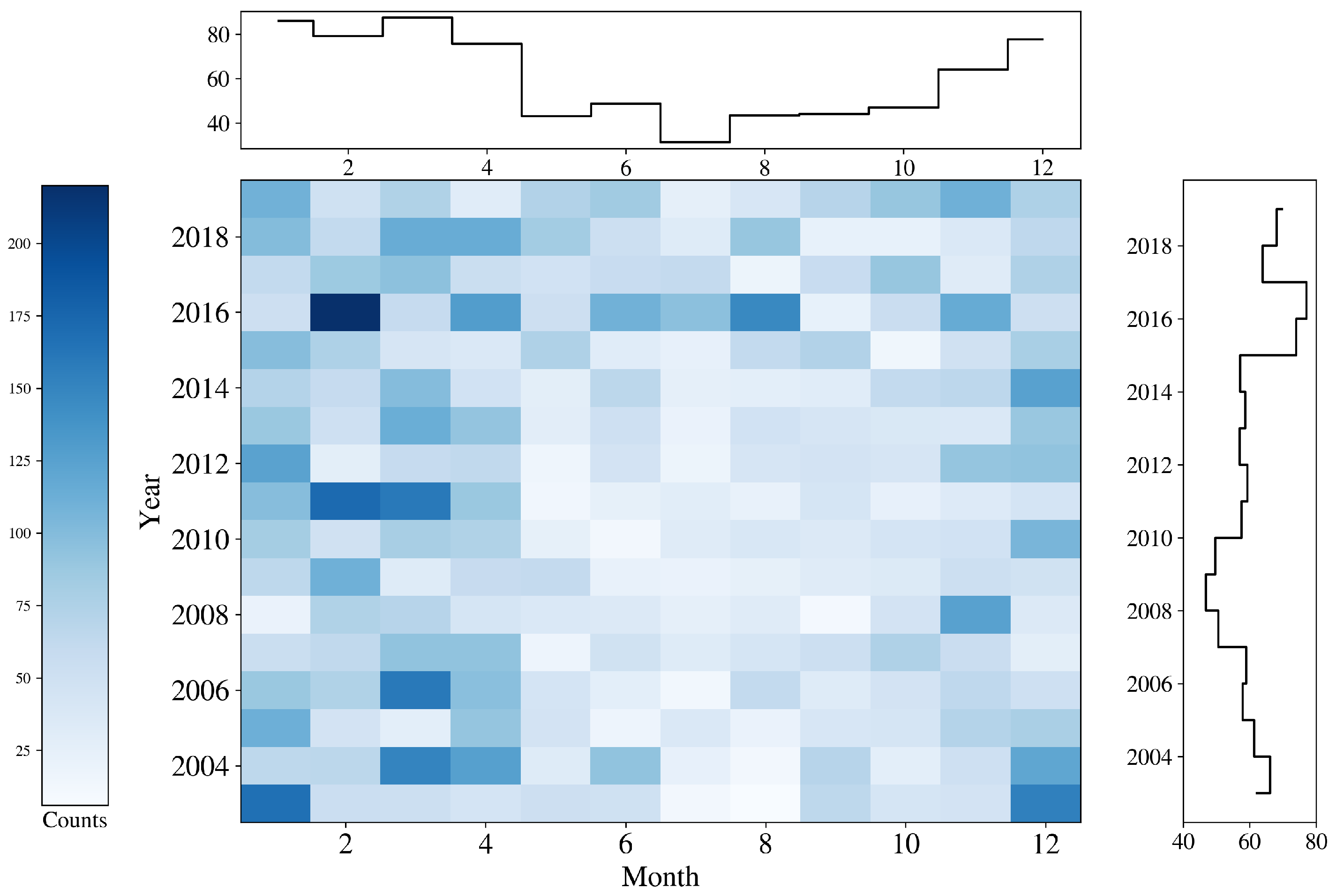
The striping apparent in the inset of Figure 4 indicates a non-uniform, temporal dependence in the outlier cutouts. Figure 5 examines this further, plotting the occurrence of outliers as a function of year and month. The only significant trend apparent is seasonal, i.e., a higher incidence of outliers during the boreal winter. We speculate this is due to the predominance of northern hemisphere cutouts/outliers—approximately 60%/64% of the total—and the reduced thermal contrast of northern hemisphere surface waters in the boreal summer. As will be shown, the range of SSTa in a cutout is correlated with the probability of the cutout being identified as an outlier; the larger the range the more likely the cutout will be so flagged. This is especially true in the vicinity of strong currents such as western boundary currents, which separate relatively warm, poleward moving equatorial and subtropical waters from cooler water poleward of the currents. In summer months the cooler water warms substantially faster than the surface water of the current dramatically reducing the contrast between the two water bodies, often masking the dynamical nature of the field in these regions rendering them less atypical. We also see variations during the ∼20 years of the full dataset, including a possible increase over the past ∼10 years. These modest trends aside, ULMO identifies outliers in all months and years of the dataset.
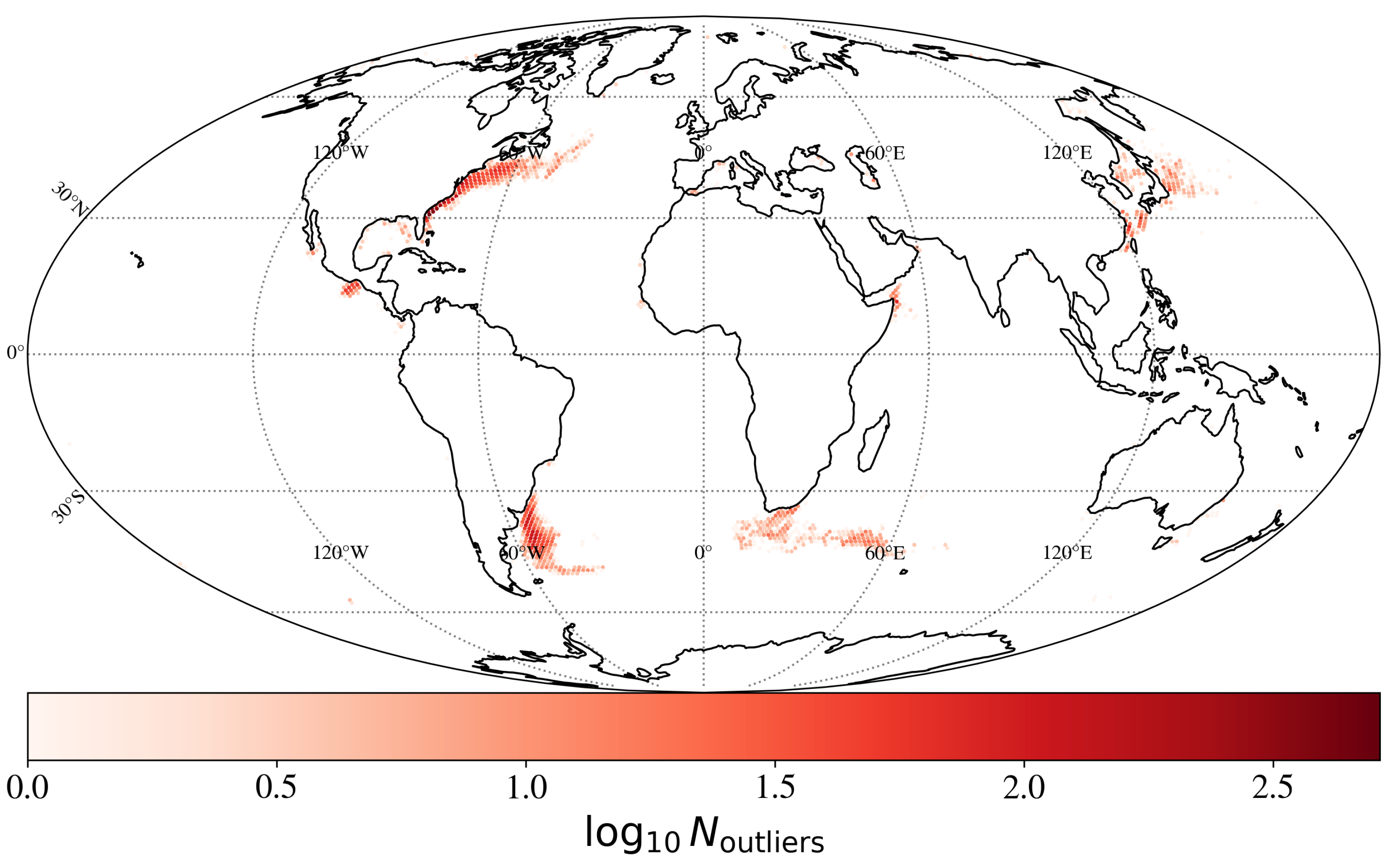
A question that naturally arises is whether there is any structure to the geographic distribution of outliers. Figure 6 shows the count distribution of the outliers across the entire ocean. Remarkably, the ULMO algorithm has rediscovered that the rarest phenomena occur primarily in western boundary currents—following the continental boundary and/or shortly after separation. These regions of the ocean have been studied extensively because of their highly dynamical nature. In short, the ULMO algorithm identified (or even rediscovered!) without any predisposition a consistent set of dynamically important oceanographic regions.
To a lesser extent, one also finds outliers in the vicinity of the connection between large gulfs or seas and the open ocean—the Gulf of California, the Red Sea and the Mediterranean. Also of interest are the outliers in the Gulf of Tehuantepec. These result from very strong winds blowing from the Gulf of Mexico to the Pacific Ocean through the Chivela Pass, resulting in significant mixing of the near-shore waters.
There are two ways to view the results in Figure 6: (1) as the contrarian, i.e., the ULMO algorithm has simply reproduced decades-old, basic knowledge in physical oceanography on where the most dynamical regions of the ocean lie; or (2) as the optimist, i.e., the ULMO algorithm—without any direction from its developers—has rederived one of the most fundamental aspects of physical oceanography. It has learned central features of the ocean from the patterns of SSTa alone. In this regard, ULMO may hold greater potential/promise to learn and derive other, not-yet-identified behaviors in the ocean.
4.2. Scrutinizing Examples of the Outliers
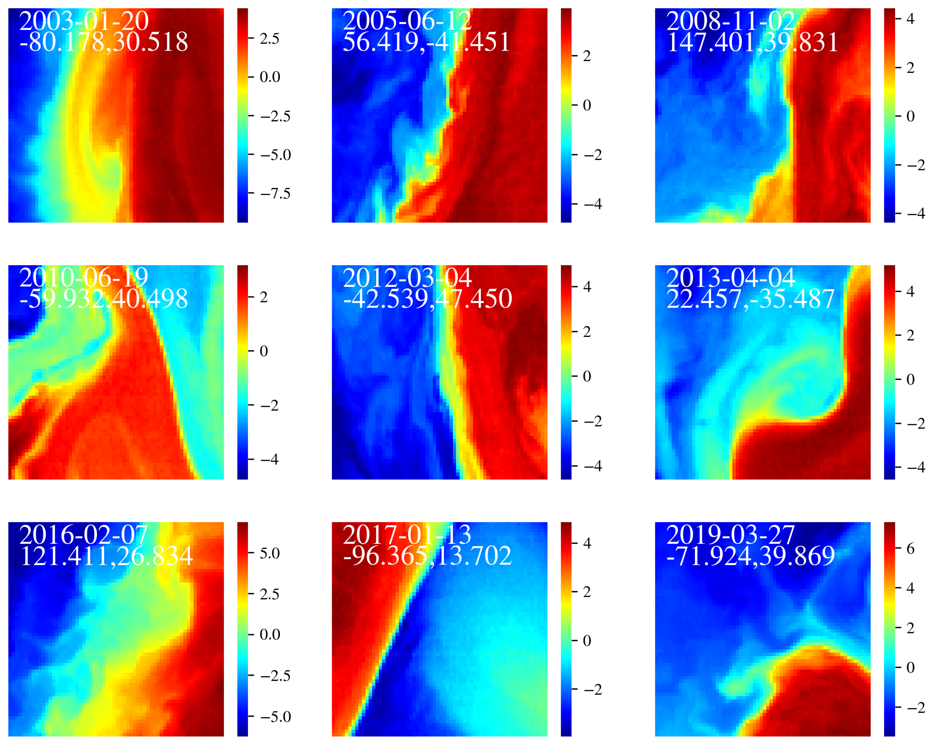
Figure 7 shows a gallery of 9 outliers selected to uniformly span time and location in the ocean. These exhibit extreme SSTa variations and/or complexity and (presumably) mark significant mesoscale activity. A common characteristic of these cutouts is the presence of a strong and sharp gradient in SSTa which separates two regions exhibiting a large temperature difference. Typically, such gradients are associated with strong ocean currents, often at mid-latitudes on the western edge of ocean basins. We define a simple statistic of the temperature distribution where is the temperature at the Xth percentile of a given cutout. All of the outliers in Figure 7 exhibit K, a point we return to in the following sub-section.
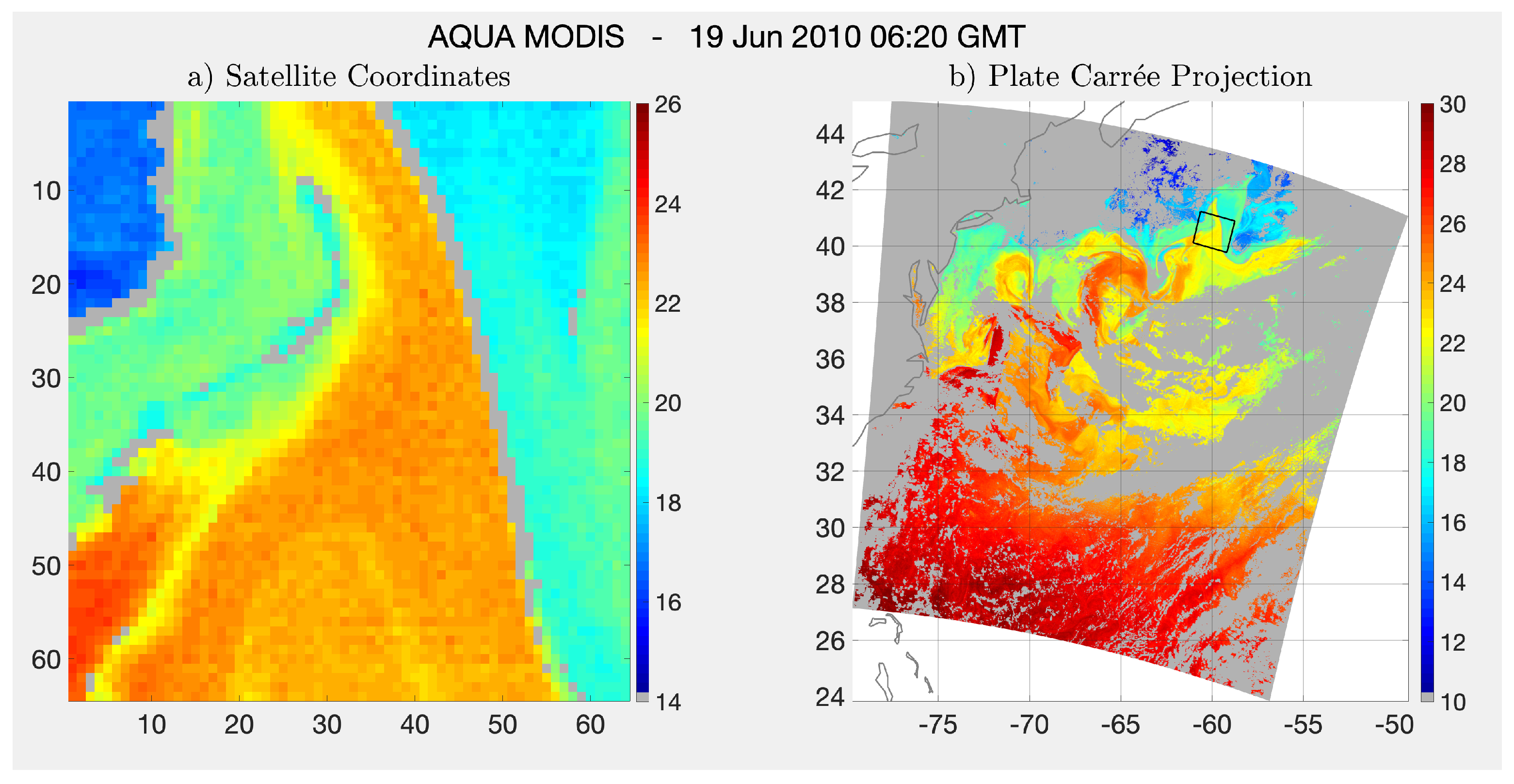
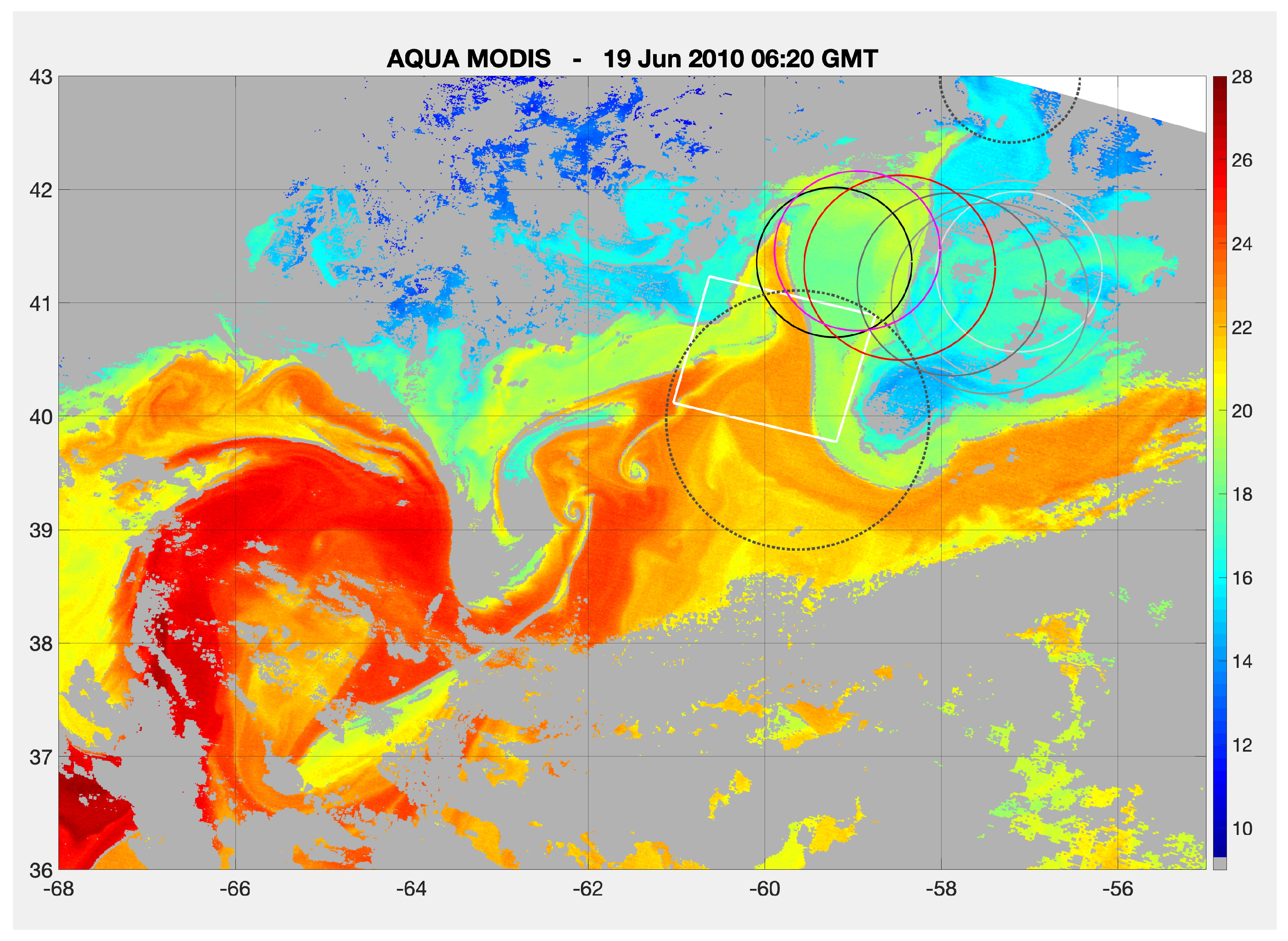
As an example of the anomalous behaviour associated with outlier cutouts, we examine the evolution of the SST field in the vicinity of the 19 June 2010 cutout (Figure 7) located in the Gulf Stream region; Figure 8a shows the cutout and (b) its location in the 5-min granule. We selected this cutout because it is in a region with which we have significant experience. Figure 9 shows an expanded version of the SST field in the vicinity of the cutout. The main feature in Figure 9 is the Gulf Stream, the bright red, fading to orange, band meandering from the bottom left hand corner of the image to the middle of the right hand side. A portion of the Gulf Stream loops through the lower half of the cutout and a streamer extends to the north (Figure 8) from the northernmost excursion of the stream. To aid in the interpretation of this cutout, we make use of the mesoscale eddy dataset produced by Chelton et al. [19]. It shows an eddy, most probably a Warm Core Ring (WCR), moving to the west at approximately 5 km/day to the north of the stream from 17 May (very light gray circle) to 14 June (red circle) when it began to interact with the Gulf Stream, drawing warm Gulf Stream Water on its western side to the north and cold Slope Water on its eastern side to the south. The eddy disappears from the altimeter record two weeks later and is replaced by a very large anticyclone (the dotted black circle) to the west southwest of the eddy’s last position. This is likely a detaching meander of the Gulf Stream resulting from the absorption of the eddy into an already chaotic configuration.
Of particular interest is that the Gulf Stream appears to have lost its coherence between approximately 63 and 59W. Specifically, note the very thin band of cooler water (∼21C) in the middle of the warm band (∼24 C) of, presumably, Gulf Stream Water between and W and a second similar band (but moving in the opposite direction) between and . The western cool band appears to separate one branch of Gulf Stream Water that has been advected from the southwestern edge of the large meander centered at W, N, and a second branch advected from its southeastern edge. These two branches may result from a general instability of the Gulf Stream associated with formation, or in this case the likely aborted formation, of a WCR. In the normal formation process, the initial state is a large meander of the Gulf Stream and the final state is a relatively straight Gulf Stream with a WCR to the north. In this case the process appears to have begun but inspection of subsequent images suggests that a ring was not formed; the the meander reformed after initially beginning the detachment process. However, this is all quite speculative, the important point is that the stream appears to have lost its coherence immediately upstream of the cutout, which we believe to be a very unusual process. Admittedly the cutout only ‘sees’ a very small portion of this but we have found the suggestion of convoluted dynamics in the immediate vicinity of a large fraction of other outliers as well. Bottom line: Cornillon, who has been looking at SST fields derived from satellite-borne sensors for over 40 years, found that more than one-in-ten of the anomalous fields discovered by ULMO suggested intriguing dynamics that he has not previously encountered; recall that this is one-in-ten of one-in-a-thousand (the definition of an outlier) or approximately one field in ten thousand.
4.3. Digging Deeper
It is evident from the preceding sub-sections (e.g., Figure 7) that ULMO has discovered a set of highly unusual and dynamic regions of the ocean. Scientifically, this is extremely useful—irrespective of the underlying processes—as it can launch future, deeper inquiry into the physical processes generating such patterns. On the other hand, as scientists we are inherently driven to understand—as best as possible—what/how/why ULMO triggered upon. We begin that process here and defer further exploration to future work.
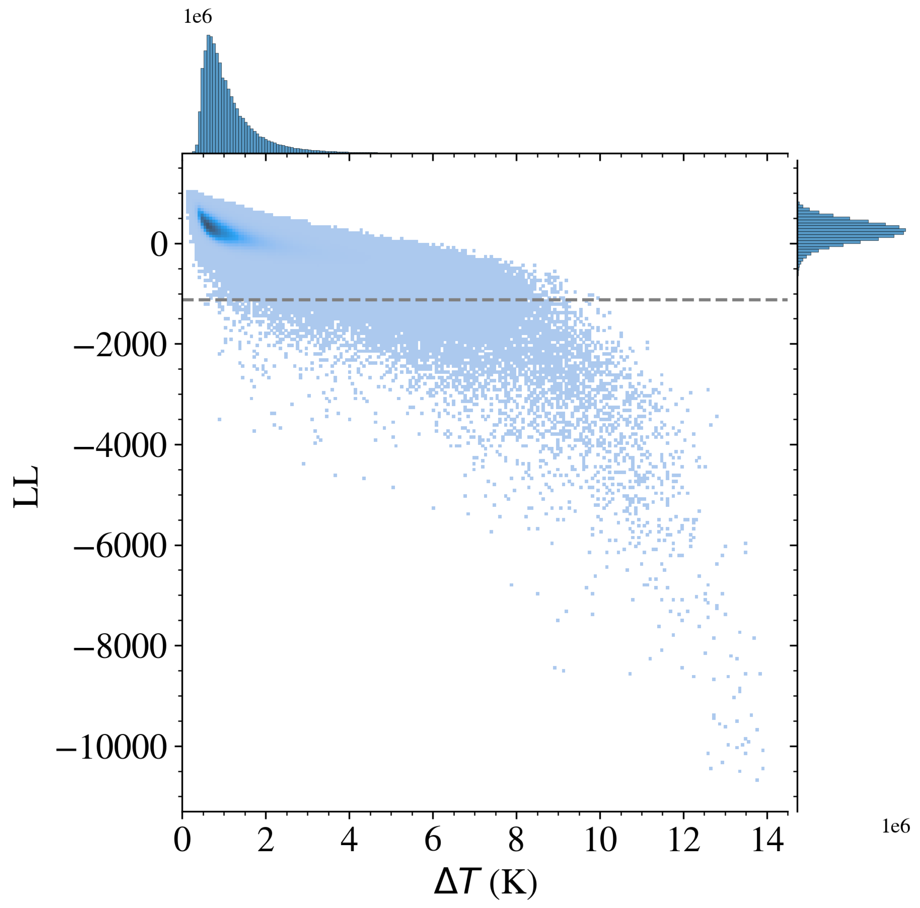
In Section 4.1, we emphasized that the entire gallery of outliers (Figure 7) exhibits a large temperature variation K. Exploring this further, Figure 10 plots LL vs. for the full set of cutouts analyzed. Indeed, the two are anti-correlated with the lowest LL values corresponding to the largest . This suggests that a simple rules-based algorithm of selecting all cutouts with K would select the most extreme outliers discovered by ULMO. One may question, therefore, whether a complex and hard-to-penetrate AI model was even necessary to reproduce our results.
Further analysis suggests that there may be more to the distribution of LLs. Specifically, note that there is substantial scatter about the mean relation between LL and ; for example, at LL one finds values ranging from 1–10 K. Similarly, any cutout with K includes a non-negligible set of images with . Figure 10 indicates that the patterns that ULMO flags as outliers are not solely determined by .
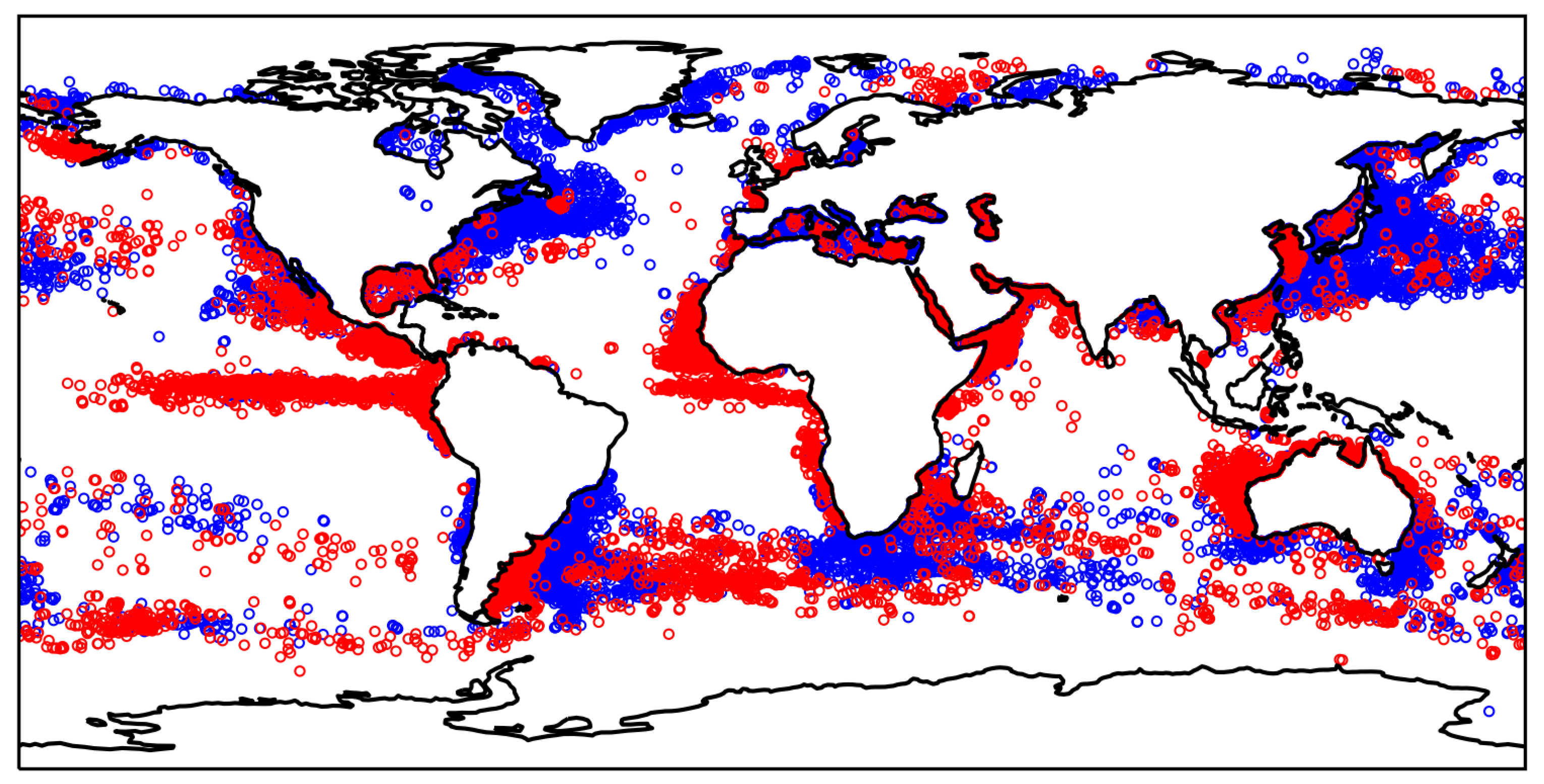
This becomes especially clear in the following exercise. Consider the full set of cutouts within the small range K. From Figure 10, we see these exhibit and find that the LL distribution is well described by a Gaussian (not shown) with and . Now consider the cutouts with the lowest/highest 10/90% of the distribution, i.e., the “outlier”/”inlier” sub-samples within this small range of . We refer to these as and cutouts, respectively. Figure 11 shows the spatial distribution of these cutouts. Remarkably, there are multiple areas dominated by only one of the sub-samples (e.g., LL cutouts along the Pacific equator). It is evident that ULMO finds large spatial structures in the log-likelihood distribution of cutouts that are independent of .
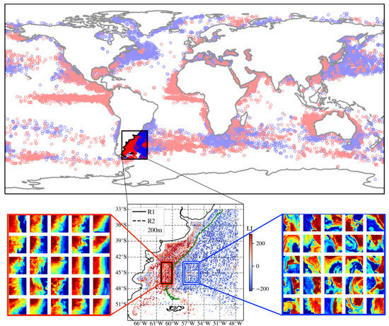
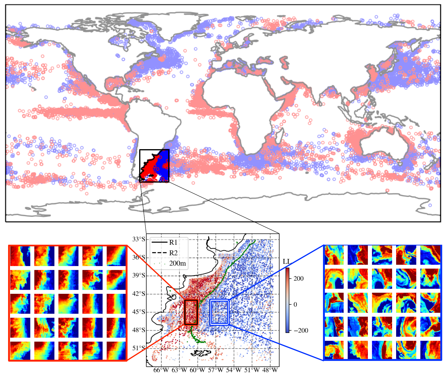
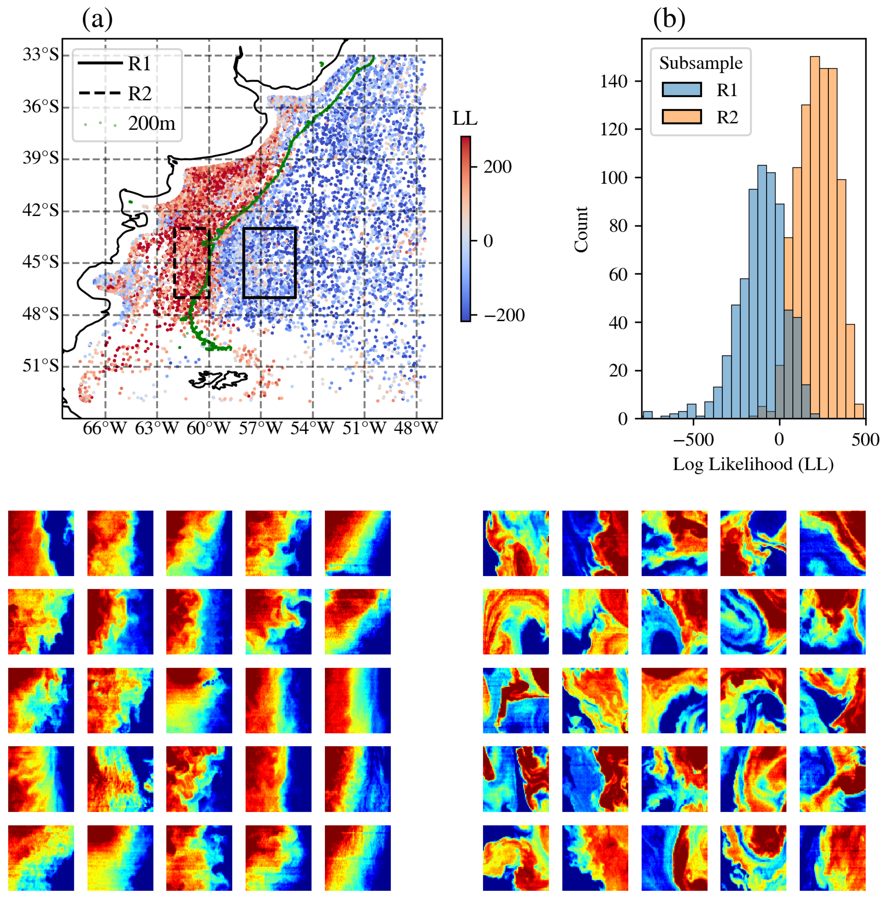
Furthermore, there are several locations in the ocean where LL and LL cutouts are adjacent to one another but still separate. One clear example is within the Brazil–Malvinas Confluence, off the coast of Argentina. Figure 12a shows a zoom-in of that region with the colors corresponding to the LL values (not strictly the LL or LL distributions shown in Figure 11). Figure 12a highlights the clear and striking separation of the LL values in this region as do the histograms (Figure 12b) for the LL values of cutouts in the two rectangles shown in panel a. The dynamics of the ocean in this region is well-studied [20]. Higher LL regions tend to be found on the Patagonian Shelf where the dynamics are dominated by tides, buoyancy and wind–forcing the circulation at the local level–and off-shore currents–forcing the circulation remotely. In contrast, the lower LL regions track more dynamic, current-driven motions of the main Brazil–Malvinas Confluence. Of particular interest is the rather abrupt switch at S from higher LL values to the south to lower values to the north. This is consistent with the observation of Combes and Matano [21], based on numerical simulations, that “there is an abrupt change of the dynamical characteristics of the shelf circulation at 40S.” They attribute this change in dynamics to this region being a sink for Patagonian Shelf waters, which are being advected offshore by the confluence of the Brazil and Malvinas Currents. Again, ULMO has captured striking detail in regional dynamics with no directed input. Further analysis of the region (not shown) suggests that ULMO has also captured seasonal differences in the dynamics, with a region of lower LL cutouts in waters approximately 100 m deep between and S in austral winter but not austral summer.
Intrigued by ULMO’s ability to spatially separate these regions based on SSTa patterns alone, we inspected a set of 25 randomly selected samples from R1, the eastern rectangle in Figure 12a and 25 randomly selected samples from R2 to further explore its inner-workings (see lower panels of Figure 12). The comparison is striking and we easily identify qualitative differences in the observed patterns despite their nearly identical values. The higher LL cutouts show large-scale gradients and features with significant coherence whereas the lower LL cutouts exhibit gradients and features with a broader range of scales and a suggested richer distribution of relative vorticity.
Another area, which stands out in Figure 11, is that in the Northwest Atlantic where a region of LL cutouts (red) are surrounded by LL cutouts (blue). The structure (not shown) of the LL cutouts in this region, which are on the Grand Banks of Newfoundland, resemble the structure of the LL cutouts shown in Figure 12 and the structure of the LL cutouts in this region is much closer to that of the LL cutouts shown in Figure 12 than to the LL cutouts in either region. In fact, a gallery of randomly selected LL cutouts from the world ocean are similar to those off of Argentina and Newfoundland and a gallery of randomly selected LL cutouts from the world ocean are more similar to the LL cutouts off of Argentina and Newfoundland than to the LL cutouts. Simply put, the structure of the SST cutouts shown in blue in Figure 11 tend to be similar to one another and quite different from those shown in red although the cutouts in both cases have virtually the same dynamic ranges in SST. This observation raises intriguing questions about the similarities and the differences in upper ocean processes in these regions—questions to be addressed in further analyses of the fields.
We can capture some of the differences between the higher/lower LL sub-samples of Figure 12 with another simple statistic—the RMS in SSTa, . On average, the lower LL cutouts exhibit ≈9% higher than those with a higher LL. Furthermore, we find LL correlates with in a fashion similar to . On the other hand, it is evident from Figure 12 that there is significant structure apparent in the cutouts that is not described solely by . The correlations of LL with and manifest from the underpinnings of ULMO: the distribution of ocean SSTa patterns reflect the distribution of simple statistics like or , which exhibit large and non-uniform variations across the ocean. The complexity of these patterns, however, belie the information provided by simple statistics alone.
5. Conclusions and Future Work
With the design and application of a machine learning algorithm ULMO, we set out to identify the rarest sea surface temperature patterns in the ocean through an out-of-distribution analysis yielding a unique log-likelihood (LL) value for every cutout. Regarding that goal, we believe we were successful (e.g., Figure 6 and Figure 7). In examining the nature of the outliers, we found that these exhibited extrema of two simple metrics: the temperature difference and standard deviation . With the full privilege of hindsight, we expect that any metric introduced to describe the cutouts which exhibits a broad and non-uniform distribution would correlate with LL. However, no single metric can capture the inherent pattern complexity, and therefore none correlates tightly with LL (Figure 10).
Looking to the future, the greatest potential of algorithms such as ULMO may be that the patterns they learn are more fundamental than measures traditionally implemented in the scientific community (e.g., Fast Fourier Transform (FFT) and Empirical Orthogonal Function EOF). We hypothesize that the mathematical nature of the CNN—convolutional features and max-pooling, which synthesize data across the scene while remaining invariant to translation—captures aspects of the data that EOF analysis could not (nor any other simple linear approach). Indeed, referring back to Figure 12, while as humans we trivially distinguish between the two sets of cutouts marking the ocean dynamics in the Brazil–Malvinas Confluence and can identify metrics by which they differ, these metrics offer incomplete descriptions. Going forward, we will determine the extent (e.g., via analysis of ocean model outputs) to which the patterns mark fundamental, dynamical processes within the ocean. Potentially, the patterns learned by ULMO (or its successors) hold the optimal description of any such phenomena.
As emphasized at the onset, this manuscript offers only a first glimpse at the potential for applying advanced artificial intelligence techniques to the tremendous ocean datasets obtained from satellite-borne sensors. The techniques introduced here will translate seemlessly to sea surface height or ocean color imaging to identify extrema/complexity in geostrophic currents and biogeochemical processes. These too will be the focus of future works.
Author Contributions
J.X.P. led the writing of the manuscript, including figure generation. He also ran the majority of the models presented. P.C.C. proposed the original idea of searching for extremes in the MODIS L2 SST dataset, undertook a significant fraction of the analysis of the resulting LL fields, guided the oceanographic interpretation of the results and contributed to the writing of the manuscript. D.M.R. prototyped and developed ULMO’s deep learning components. All authors have read and agreed to the published version of the manuscript.
Funding
J.X.P. recognizes support from the University of California, Santa Cruz. Support for PC was provided by the Office of Naval Research: ONR N00014-17-1-2963 and NASA grant # 80NSSC18K0837
Acknowledgments
MODIS SST data were produced by and obtained from the NASA Goddard Space Flight Center, Ocean Ecology Laboratory, Ocean Biology Processing Group; bathymetry was obtained from the GEBCO Compilation Group (2020) GEBCO 2020 Grid (doi: 10.5285/a29c5465-b138-234d-e053-6c86abc040b9); the authors gratefully acknowledge helpful discussions with Baylor Fox-Kemper of Brown University, Chris Edwards of UC Santa Cruz and Peter Minnett and Kay Kilpatrick of the University of Miami.
Conflicts of Interest
The authors declare no conflict of interest.
Abbreviations
| CC | cloud cover |
| CNN | Convolutional Neural Network |
| EOF | Empirical Orthogonal Function |
| FFT | Fast Fourier Transform |
| GSFC | Goddard Space Flight Center |
| L2 | Level-2 |
| LL | log-likelihood |
| MODIS | MODerate-resolution Imaging Spectroradiometer |
| NASA | National Aeronautics and Space Administration |
| OBPG | Ocean Biology Processing Group |
| ONR | Office of Naval Research |
| OOD | out-of-distribution |
| PAE | probabilistic autoencoder |
| PCA | Principal Components Analysis |
| probability distribution function | |
| SSH | sea surface height |
| SST | sea surface temperature |
| SSTa | SSTa |
| URI | University of Rhode Island |
| WCR | Warm Core Ring |
Appendix A

Table A1.
Model and training hyperparameters, where the leftmost column lists the variable name, the middle column offers a brief description of the hyperparameter’s function and the rightmost column lists the value we used in our final model. Note that all autoencoder architecture hyperparameters refer to the encoder-side only (as the decoder is unused after training).
| Hyperparameter | Description | Value |
|---|---|---|
| n_conv_layers | Number of convolutional layers in autoencoder | 4 |
| kernel_size | Size of kernel in convolutional layers | 3 |
| stride | Stride in convolutional layers | 2 |
| out_channels | Number of output channels in convolutional layers | for i the layer index |
| n_latent | Dimension of the autoencoder latent space | 512 |
| n_flow_layers | Number of coupling layers in flow | 10 |
| hidden_units | Number of hidden units in flow layers | 256 |
| n_blocks | Number of residual blocks per flow layer | 2 |
| dropout | Dropout probability in flow layers | 0.2 |
| use_batch_norm | Use batch normalization in flow layers | False |
| conv_lr | Autoencoder learning rate | 2.5 × 10⁻³ |
| flow_lr | Flow learning rate | 2.5 × 10⁻⁴ |
References
- Prochaska, J.X.; Reiman, D. Available online: https://github.com/AI-for-Ocean-Science/ulmo (accessed on 16 February 2021).
- GHRSST Project Office. Available online: https://www.ghrsst.org/ghrsst-data-services/products/ (accessed on 16 February 2021).
- Abul Hayat, M.; Stein, G.; Harrington, P.; Lukić, Z.; Mustafa, M. Self-Supervised Representation Learning for Astronomical Images. arXiv 2020, arXiv:2012.13083. [Google Scholar]
- Saux Picart, S.; Tandeo, P.; Autret, E.; Gausset, B. Exploring Machine Learning to Correct Satellite-Derived Sea Surface Temperatures. Remote Sens. 2018, 10, 224. [Google Scholar] [CrossRef] [Green Version]
- Paul, S.; Huntemann, M. Improved machine-learning based open-water/sea-ice/cloud discrimination over wintertime Antarctic sea ice using MODIS thermal-infrared imagery. Cryosphere Discuss. 2020, 2020, 1–23. [Google Scholar] [CrossRef]
- Moschos, E.; Schwander, O.; Stegner, A.; Gallinari, P. DEEP-SST-EDDIES: A Deep Learning framework to detect oceanic eddies in Sea Surface Temperature images. In Proceedings of the ICASSP 2020—45th International Conference on Acoustics, Speech, and Signal Processing, Barcelona, Spain, 4–8 May 2020. [Google Scholar]
- Ratnam, J.V.; Dijkstra, H.A.; Behera, S.K. A machine learning based prediction system for the Indian Ocean Dipole. Sci. Rep. 2020, 10, 284. [Google Scholar] [CrossRef] [PubMed] [Green Version]
- Zhang, Z.; Pan, X.; Jiang, T.; Sui, B.; Liu, C.; Sun, W. Monthly and Quarterly Sea Surface Temperature Prediction Based on Gated Recurrent Unit Neural Network. J. Mar. Sci. Eng. 2020, 8, 249. [Google Scholar] [CrossRef] [Green Version]
- Yu, X.; Shi, S.; Xu, L.; Liu, Y.; Miao, Q.; Sun, M. A Novel Method for Sea Surface Temperature Prediction Based on Deep Learning. Math. Probl. Eng. 2020, 2020, 6387173. [Google Scholar] [CrossRef]
- Ma, L.; Liu, Y.; Zhang, X.; Ye, Y.; Brian Alan Johnson, G.Y. Deep learning in remote sensing applications: A meta-analysis and review. ISPRS J. Photogramm. Remote Sens. 2019, 152, 166–177. [Google Scholar] [CrossRef]
- Nalisnick, E.; Matsukawa, A.; Teh, Y.W.; Gorur, D.; Lakshminarayanan, B. Do deep generative models know what they don’t know? arXiv 2018, arXiv:1810.09136. [Google Scholar]
- Minnett, P.J.; Kilpatrick, K.; Szczodrak, G.; Izaguirre, M.; Luo, B.; Jia, C.; Proctor, C.; Bailey, S.W.; Armstrong, E.; Vazquez-Cuervo, J.; et al. MODIS Sea-Surface Temperatures: Characteristics of the R2019.0 Reprocessing of the Terra and Aqua Missions. In Proceedings of the 21st International GHRSST Science Team On-Line Meeting, Boulder, CO, USA, 1–4 June 2020; pp. 24–30. [Google Scholar]
- Kilpatrick, K.A.; Podestá, G.; Williams, E.; Walsh, S.; Minnett, P.J. Alternating Decision Trees for Cloud Masking in MODIS and VIIRS NASA Sea Surface Temperature Products. J. Atmos. Ocean. Technol. 2019, 36, 387–407. [Google Scholar] [CrossRef]
- Szegedy, C.; Ioffe, S.; Vanhoucke, V.; Alemi, A.A. Inception-v4, Inception-ResNet and the Impact of Residual Connections on Learning. In Proceedings of the ICLR 2016 Workshop, San Juan, Puerto Rico, 2–4 May 2016. [Google Scholar]
- Bertalmio, M.; Bertozzi, A.L.; Sapiro, G. Navier-stokes, fluid dynamics, and image and video inpainting. In Proceedings of the 2001 IEEE Computer Society Conference on Computer Vision and Pattern Recognition, CVPR 2001, Kauai, HI, USA, 8–14 December 2001. [Google Scholar] [CrossRef] [Green Version]
- Qiu, B.; Chen, S.; Klein, P.; Torres, H.; Wang, J.; Fu, L.L.; Menemenlis, D. Reconstructing Upper-Ocean Vertical Velocity Field from Sea Surface Height in the Presence of Unbalanced Motion. J. Phys. Oceanogr. 2019, 50, 55–79. [Google Scholar] [CrossRef]
- Durkan, C.; Bekasov, A.; Murray, I.; Papamakarios, G. Neural spline flows. arXiv 2019, arXiv:1906.04032. [Google Scholar]
- Kingma, D.P.; Welling, M. Auto-encoding variational bayes. arXiv 2013, arXiv:1312.6114. [Google Scholar]
- Chelton, D.B.; Schlax, M.G.; Samelson, R.M. Global observations of nonlinear mesoscale eddies. Prog. Oceanogr. 2011, 91, 167–216. [Google Scholar] [CrossRef]
- Piola, A.R.; Palma, E.D.; Bianchi, A.A.; Castro, B.M.; Dottori, M.; Guerrero, R.A.; Marrari, M.; Matano, R.P.; Möller, O.O., Jr.; Saraceno, M. Physical Oceanography of the SW Atlantic Shelf: A Review. In Plankton Ecology of the Southwestern Atlantic; Springer International Publishing: Cham, Switzerland, 2018; pp. 37–56. [Google Scholar]
- Combes, V.; Matano, R.P. The Patagonian shelf circulation: Drivers and variability. Prog. Oceanogr. 2018, 167, 24–43. [Google Scholar] [CrossRef]
Figure 1.
Mollweide projection depicting the log of the spatial distribution of all cutouts analyzed in this manuscript. Note the higher incidence of data closer to land driven by the lower cloud cover (CC) in those areas.
Figure 1.
Mollweide projection depicting the log of the spatial distribution of all cutouts analyzed in this manuscript. Note the higher incidence of data closer to land driven by the lower cloud cover (CC) in those areas.

Figure 2.
(left) Cutout which shows masking (white pixels) due primarily to sharp temperature gradients in this case, which tend to be flagged as low quality by the standard MODIS processing algorithm. (right) Same image but with masked pixels replaced by estimated values using the Navier-Stokes in-painting algorithm.

Figure 3.
(left) Input cutout, preprocessed as described in Section 3.1. (right) Image generated by the trained autoencoder, which passed the cutout through a 512 unit latent space. As designed, the reproduction captured the gross features but not all of the small-scale detail.
Figure 3.
(left) Input cutout, preprocessed as described in Section 3.1. (right) Image generated by the trained autoencoder, which passed the cutout through a 512 unit latent space. As designed, the reproduction captured the gross features but not all of the small-scale detail.

Figure 4.
Distribution of log-likelihood (LL) values for the full dataset (modulo the training images). The majority are well described by a Gaussian centered at , with a tail toawrd much lower LL values. The inset shows the lowest 0.1% sample of LL, which we define as outlier cutouts.
Figure 4.
Distribution of log-likelihood (LL) values for the full dataset (modulo the training images). The majority are well described by a Gaussian centered at , with a tail toawrd much lower LL values. The inset shows the lowest 0.1% sample of LL, which we define as outlier cutouts.

Figure 5.
Incidence (counts) of outlier cutouts broken down by month and year. The primary feature is seasonal, i.e., a higher number of outlier cutouts during boreal winter months than summer. There was also a weak but plausible increase in the incidence of outliers over the past years.
Figure 5.
Incidence (counts) of outlier cutouts broken down by month and year. The primary feature is seasonal, i.e., a higher number of outlier cutouts during boreal winter months than summer. There was also a weak but plausible increase in the incidence of outliers over the past years.

Figure 6.
Depiction of the spatial distribution of the outliers discovered by ULMO. These are primarily in the well-known western boundary currents off Japan, North and South America and South Africa. Note that the scaling is logarithmic.
Figure 6.
Depiction of the spatial distribution of the outliers discovered by ULMO. These are primarily in the well-known western boundary currents off Japan, North and South America and South Africa. Note that the scaling is logarithmic.

Figure 7.
Gallery of outliers drawn from the distribution of cutouts with the lowest 0.1% of LL values. This representative sample was further selected to uniformly sample the year interval of the dataset and the spatial distribution (Figure 6). Note the large and complex temperature gradients within all cutouts showing K. The color bar refers to SSTa in units of Kelvin.

Figure 8.
The 19 June 2010 cutout of Figure 7 with LL , in the lowest 0.1% of the log-likelihood values for the dataset. (a) The original cutout in satellite-coordinates prior to preprocessing. (b) The entire granule shown in a plate carrée projection with the continental boundary (dark gray) and the cutout (black rectangle). Note the change of palettes from (a) to (b) to accommodate the larger range of sea surface temperature (SST) in (b). Light gray are masked pixels, from clouds, land or clear pixels improperly flagged as cloud-contaminated (Section 2).

Figure 9.
The SST field in the vicinity of the 19 June 2010 cutout of Figure 7. The cutout (white rectangle) is centered on 60W, 4130″N. Solid circles outline all observations of the anticyclonic eddy identified by Chelton et al. [19], which passed through the cutout on 19 June 2010. Circles are colored from light gray (1st detection of the eddy on 17 May) to black (last observation on 28 June) with the exceptions of its location shown in red on 14 June, immediately prior to the satellite overpass, and its location (magenta) one week later, 21 June, immediately following the overpass. Circles with dotted black outlines are anticyclonic eddies found in a broader search ( centered on 60W, 4130N) on 5 July, one week after the last observation of the eddy of interest. No cyclonic eddies were found in a similar search. Clouds are light gray.

Figure 10.
Distribution of LL values as a function of . While there is a strong anti-correlation, the relationship exhibits substantial scatter such that is not a precise predictor of LL nor the underlying SSTa patterns characterized by ULMO. The horizontal line at corresponds to the 0.1% threshold; cutouts with log-likelihood values beneath this line are considered to be outliers.

Figure 11.
Spatial distribution of the LL/LL cutouts (red/blue) defined as the upper/lower tenth percentiles of the LL distribution for the set of cutouts with K. It is evident that these cutouts occupy distinct regions of the ocean; i.e., the ULMO algorithm has identified patterns with significant spatial coherence. More remarkably, note several areas (e.g., in the Brazil–Malvinas current) where one identifies adjacent but separate patches of LL and LL cutouts.

Figure 12.
(a) Distribution of the LL values for cutouts near the Brazil–Malvinas Confluence, restricted to those with K. One can identify a clear separation, where the lower LL values lie within the current and the higher values lie close to the Argentinian coast. Marked are two rectangles (R1 and R2), one in each region, referred to in the other panels. Marked also is the 200 m bathymetry described in the text. (b) Histograms of the LL values for the cutouts from two regions (R1/R2) chosen to show lower/higher LL values near the confluence. (lower panels) Representative cutouts from each subset—the left set was drawn from the R2 rectangle and therefore exhibit higher LL values. The right set was from R1. These galleries reveal qualitative differences in the SST patterns, i.e., unique ocean dynamics. The palette for the lower panels ranges linearly from to 1 K.

Publisher’s Note: MDPI stays neutral with regard to jurisdictional claims in published maps and institutional affiliations. |
© 2021 by the authors. Licensee MDPI, Basel, Switzerland. This article is an open access article distributed under the terms and conditions of the Creative Commons Attribution (CC BY) license (http://creativecommons.org/licenses/by/4.0/).
Share and Cite
MDPI and ACS Style
Prochaska, J.X.; Cornillon, P.C.; Reiman, D.M. Deep Learning of Sea Surface Temperature Patterns to Identify Ocean Extremes. Remote Sens. 2021, 13, 744. https://0-doi-org.brum.beds.ac.uk/10.3390/rs13040744
AMA Style
Prochaska JX, Cornillon PC, Reiman DM. Deep Learning of Sea Surface Temperature Patterns to Identify Ocean Extremes. Remote Sensing. 2021; 13(4):744. https://0-doi-org.brum.beds.ac.uk/10.3390/rs13040744
Chicago/Turabian StyleProchaska, J. Xavier, Peter C. Cornillon, and David M. Reiman. 2021. "Deep Learning of Sea Surface Temperature Patterns to Identify Ocean Extremes" Remote Sensing 13, no. 4: 744. https://0-doi-org.brum.beds.ac.uk/10.3390/rs13040744
Note that from the first issue of 2016, this journal uses article numbers instead of page numbers. See further details here.