
Machine Learning Comparison and Parameter Setting Methods for the Detection of Dump Sites for Construction and Demolition Waste Using the Google Earth Engine

 ,
,  ,
,  ,
, 
Abstract
:
1. Introduction
2. Study Areas and Datasets
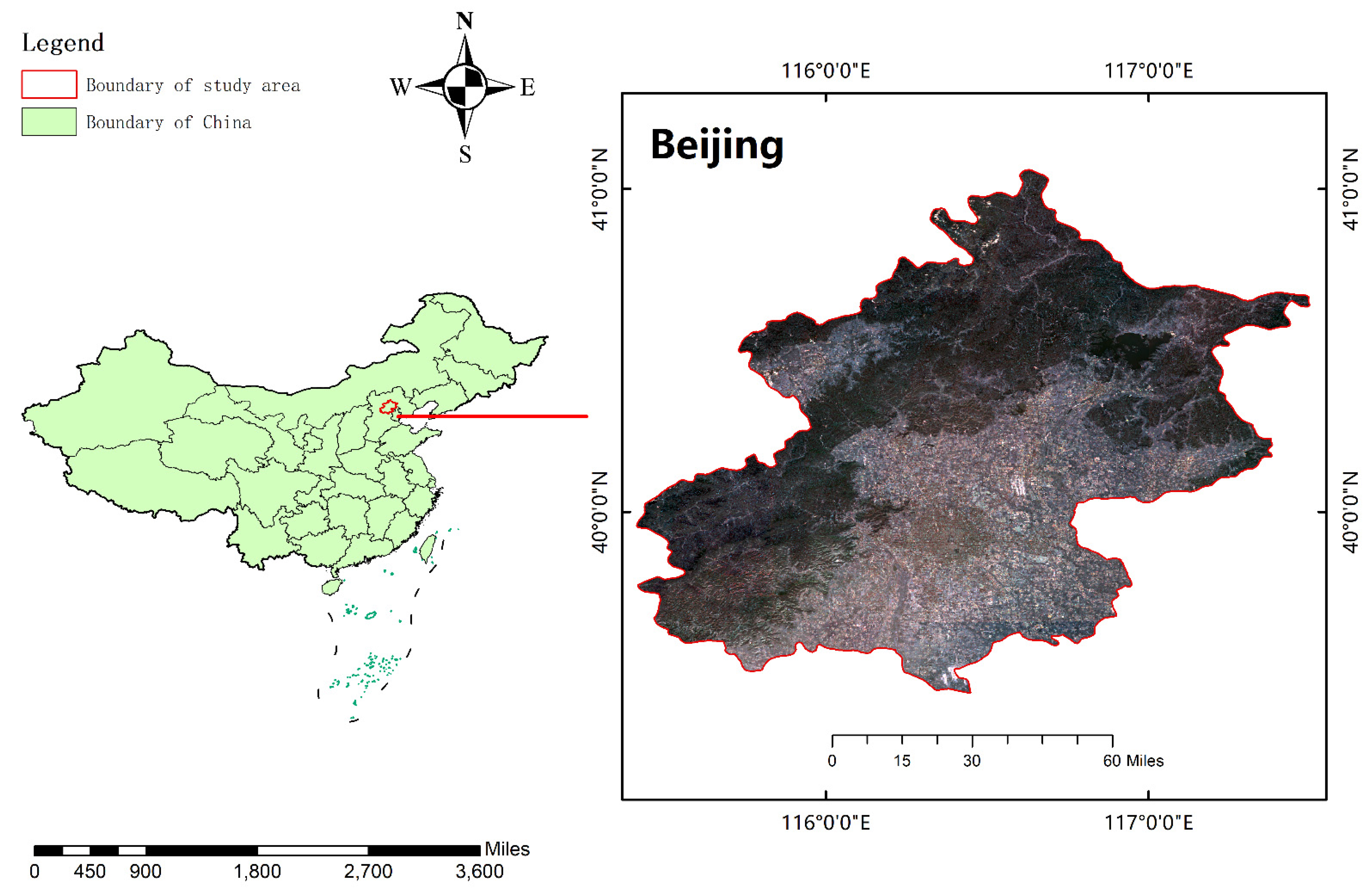
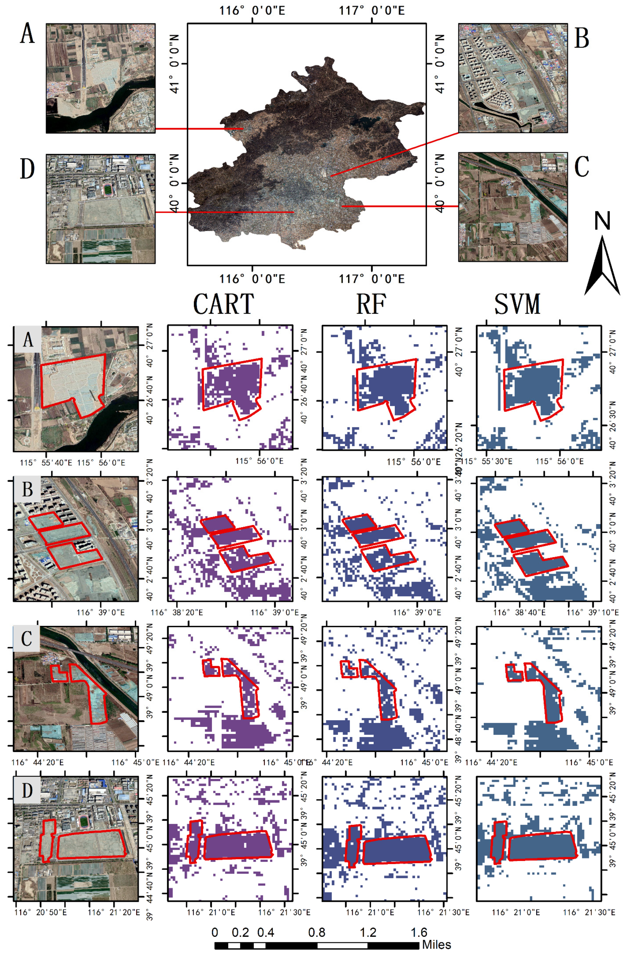
2.1. Study Area
2.2. Data Source
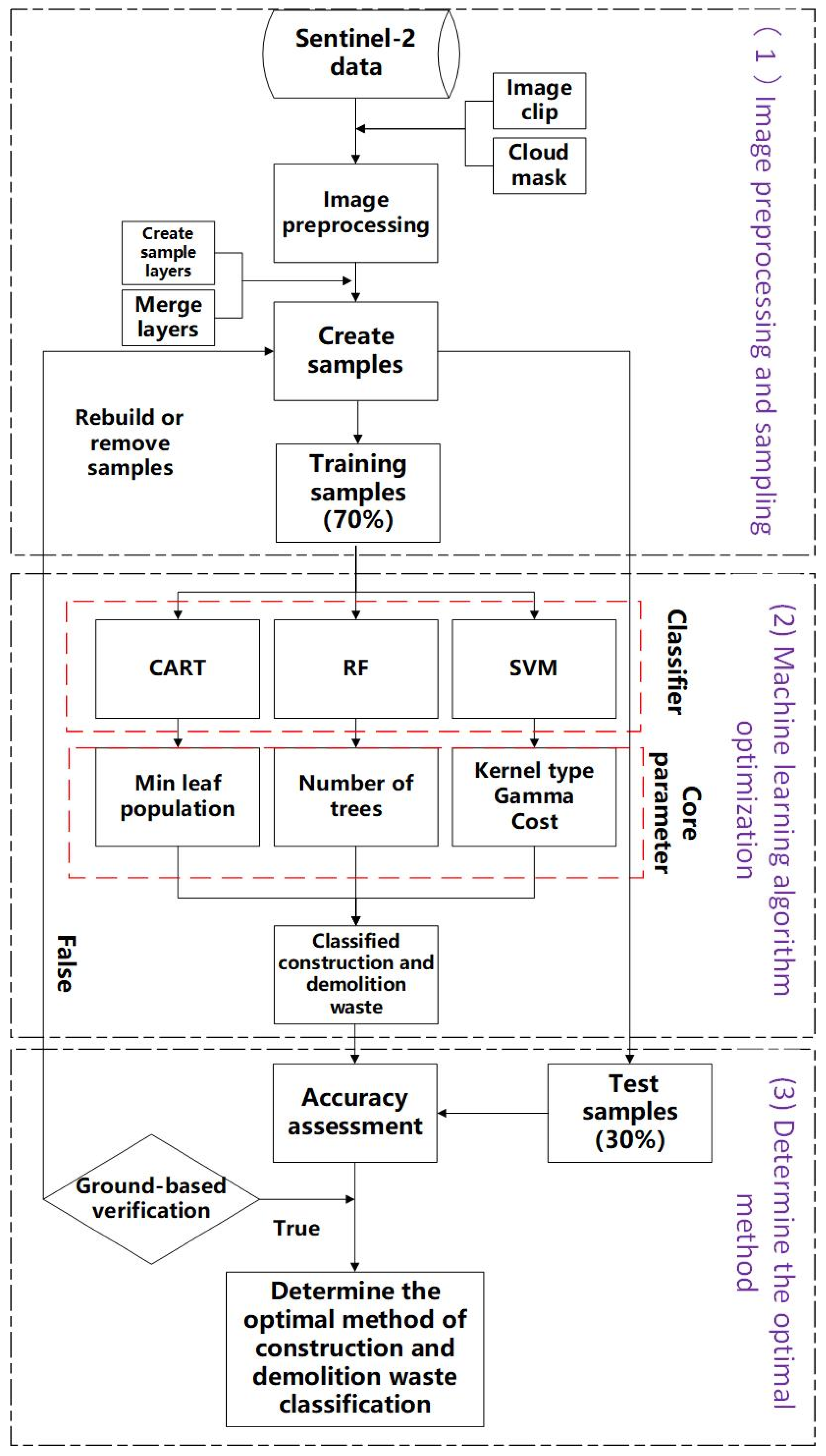
3. Methods
3.1. Sampling
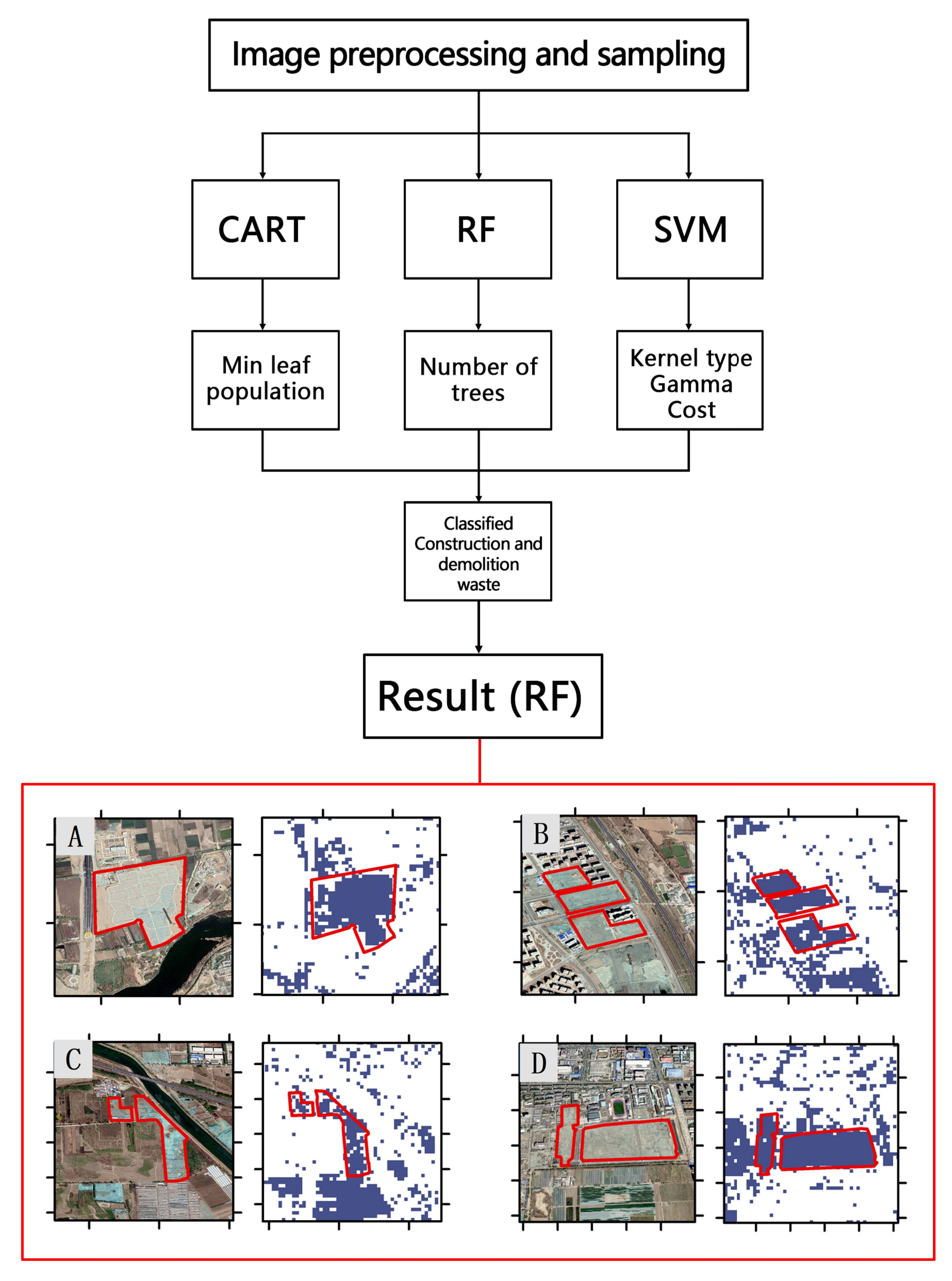
3.2. Machine Learning
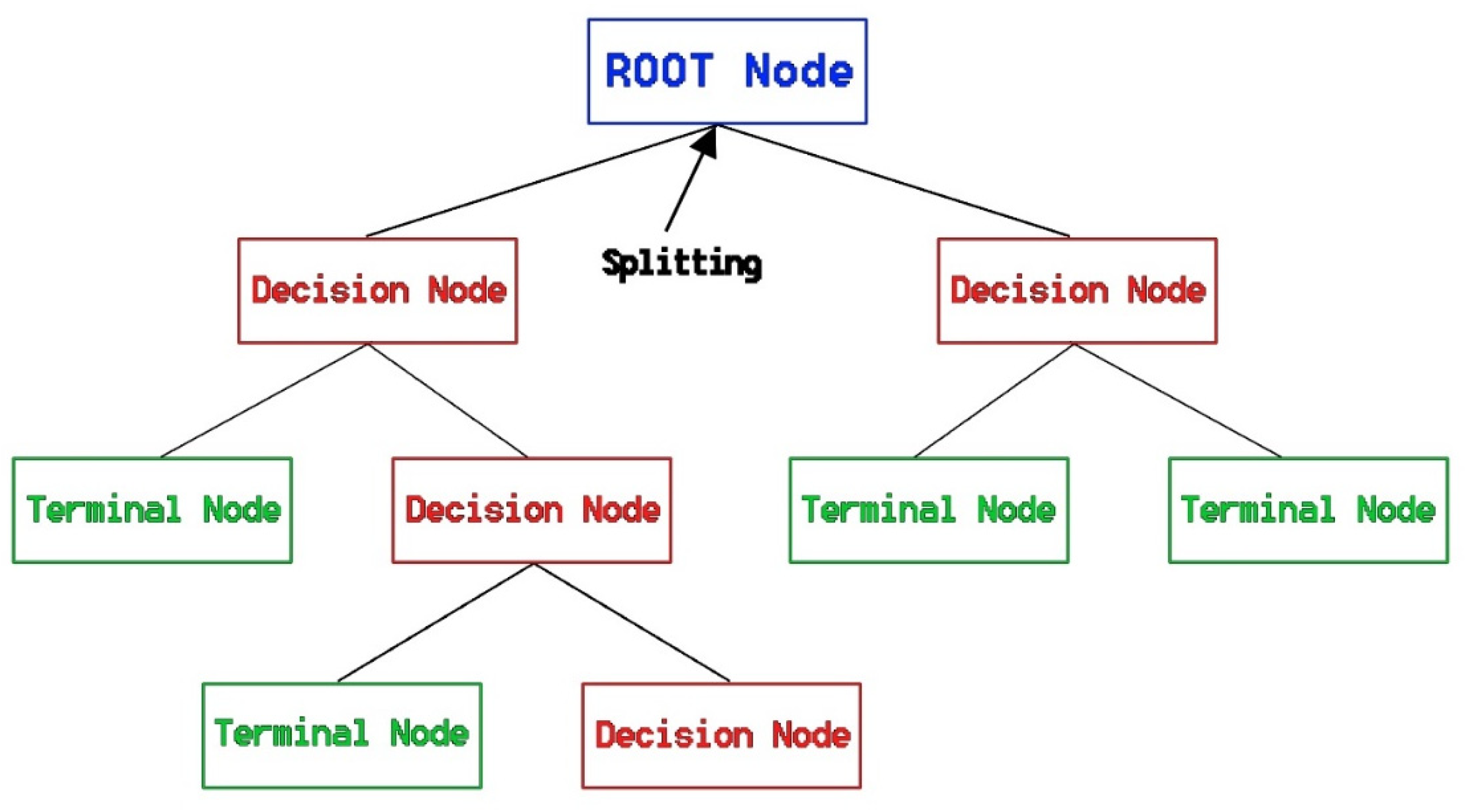
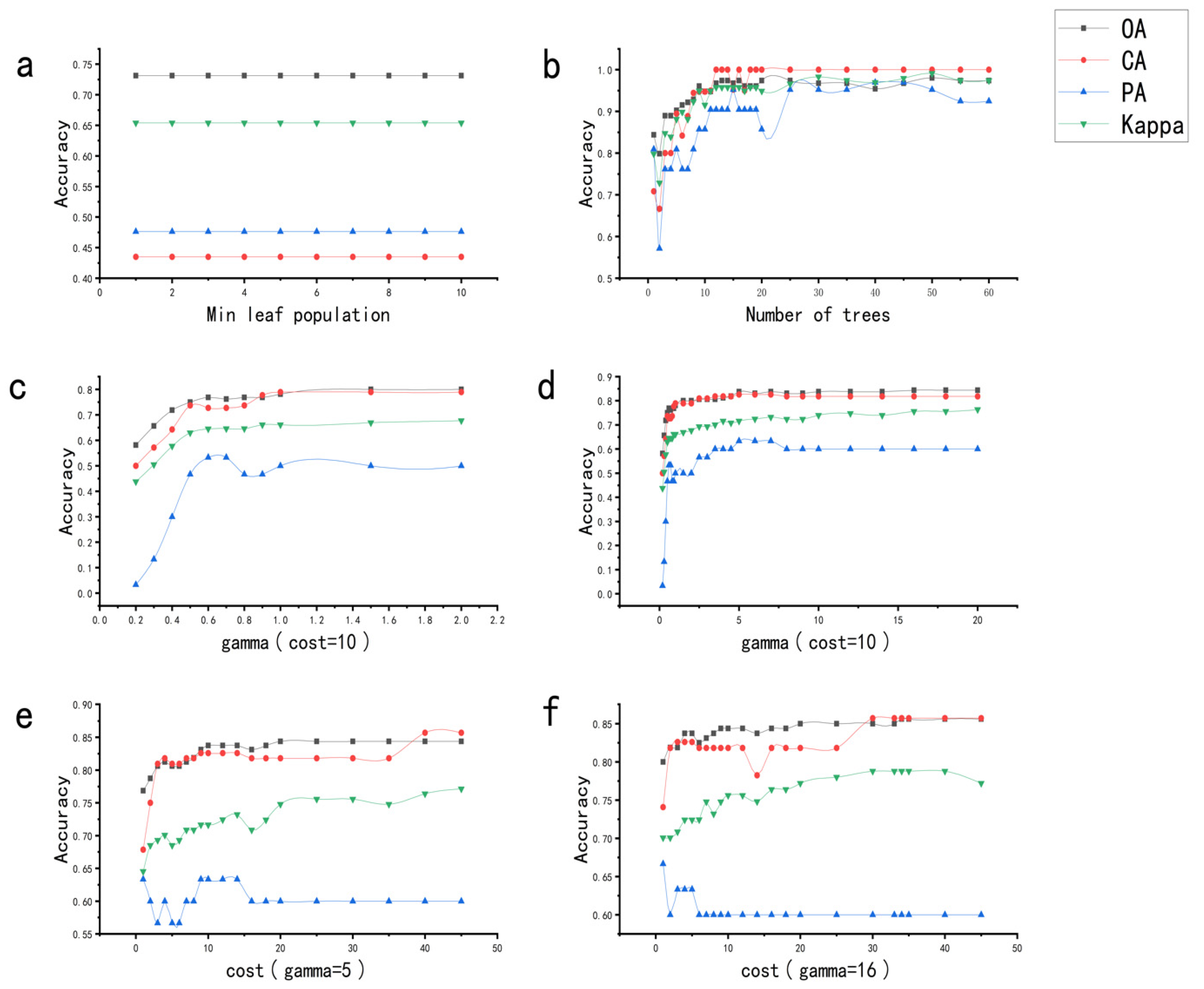
3.2.1. CART and Parametric Optimization Scheme
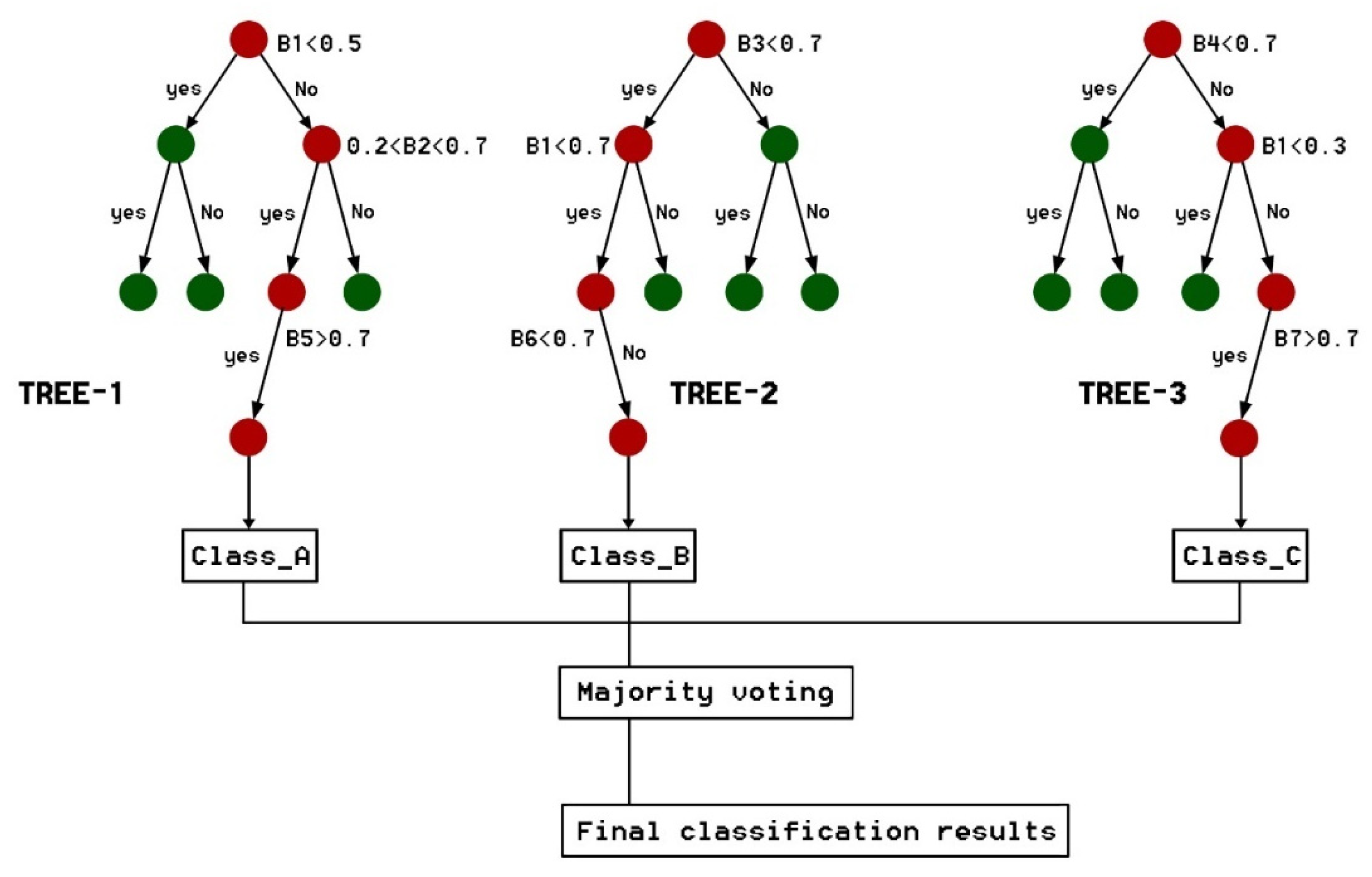
3.2.2. RF and Parametric Optimization Scheme
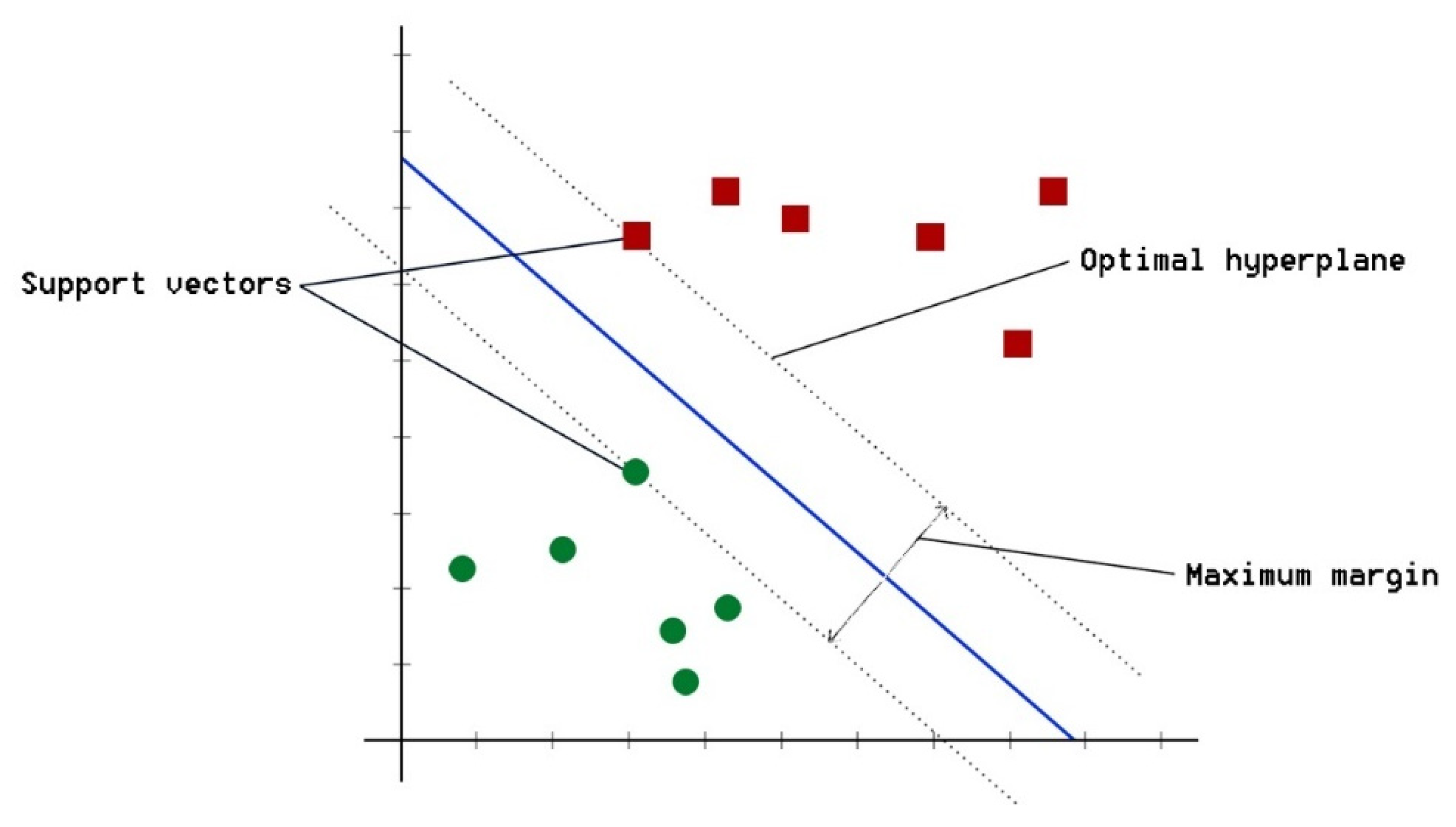
3.2.3. SVM and Parametric Optimization Scheme
- Polynomial kernel:where is the polynomial order and and are artificially defined parameters.
- Radial basis function (RBF) kernel:where is greater than 0 and defined manually.
- SIGmoID kernel.where is the upsilon, a manually defined parameter.
3.3. Verification Methods
4. Results and Analysis
4.1. Accuracy Assessment
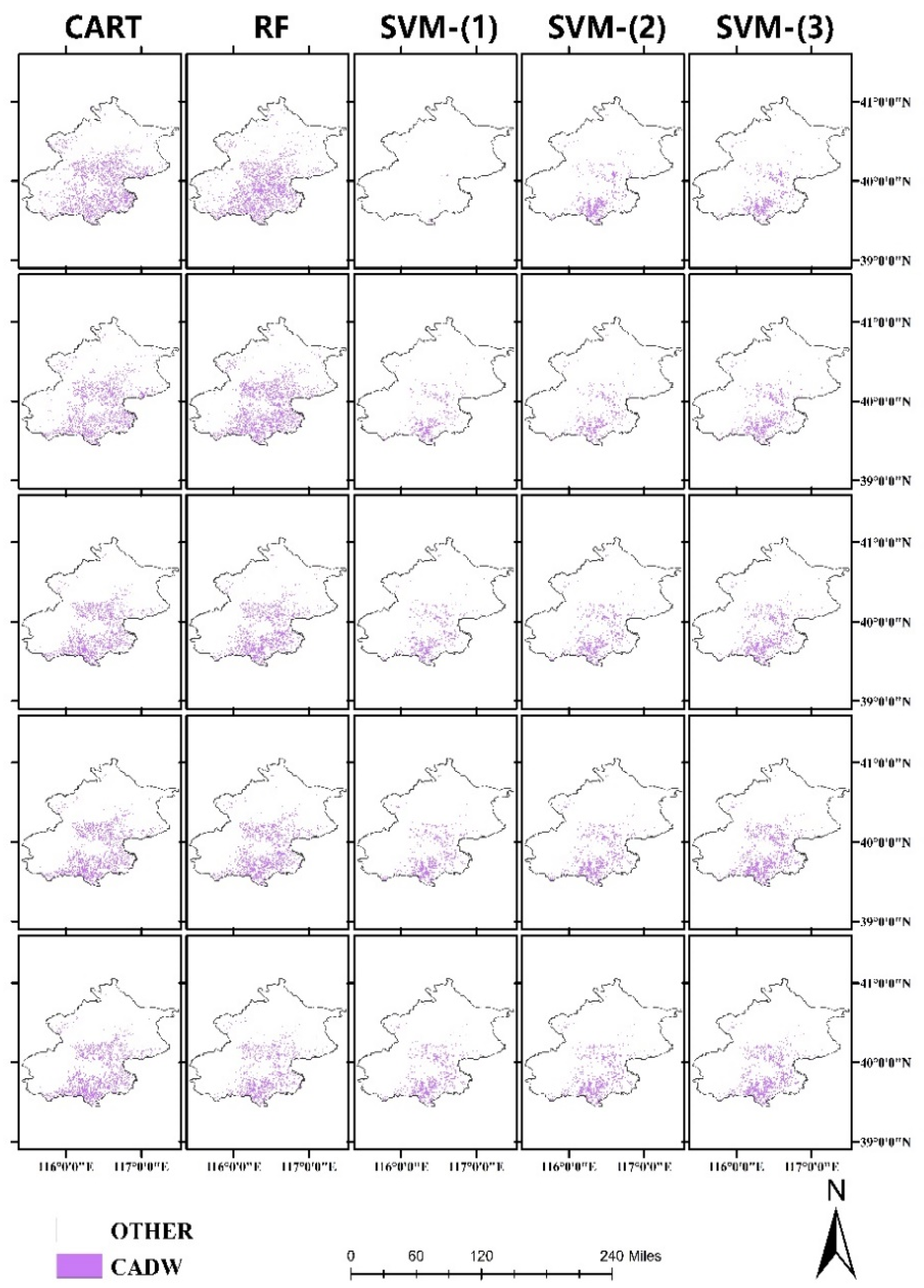
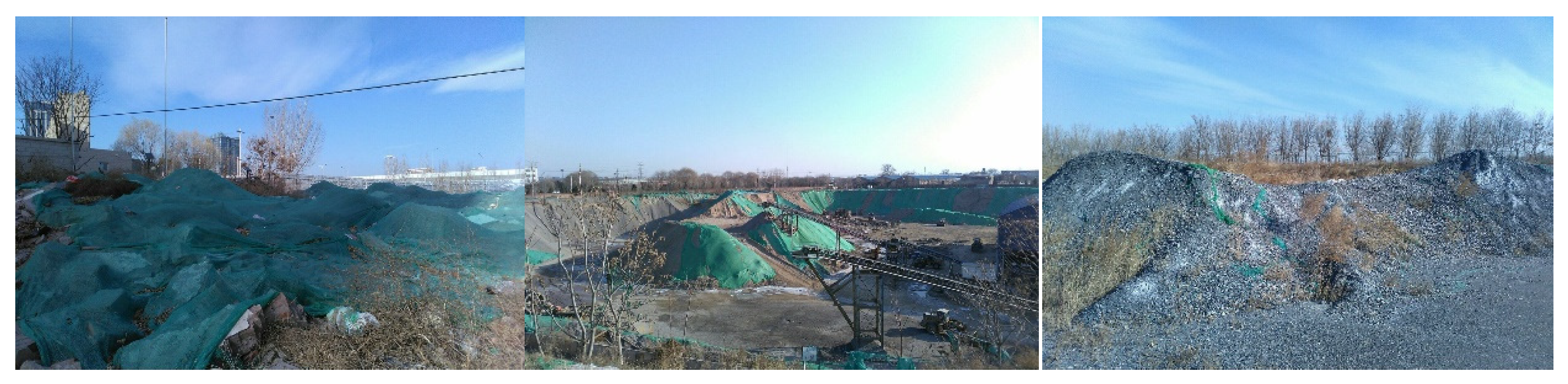
4.2. Ground Verification
5. Discussion and Conclusions
Supplementary Materials
Author Contributions
Funding
Acknowledgments
Conflicts of Interest
References
- Zhou, W.; Chen, J.; Lu, H. Status And Countermeasures Of Domestic Construction Waste Resources. Archit. Technol. 2009, 40, 741–744. [Google Scholar]
- Huang, B.; Wang, X.; Kua, H.; Geng, Y.; Bleischwitz, R.; Ren, J. Construction and demolition waste management in China through the 3R principle. Resour. Conserv. Recycl. 2018, 129, 36–44. [Google Scholar] [CrossRef]
- Zhou, Z.H.; Su, Z. Current Situation and Measures of Construction Waste Treatment. Sci. Technol. Innov. 2019, 07, 114–115. [Google Scholar]
- Yazdani, M.; Kabirifar, K.; Frimpong, B.E.; Shariati, M.; Mirmozaffari, M.; Boskabadi, A. Improving construction and demolition waste collection service in an urban area using a simheuristic approach: A case study in Sydney, Australia. J. Clean. Prod. 2021, 280, 124138. [Google Scholar] [CrossRef]
- Ma, M.; Tamm, V.W.Y.; Le, K.N. Challenges in current construction and demolition waste recycling: A China study. Waste Manag. 2020, 118, 610–625. [Google Scholar] [CrossRef]
- Oh, D.; Noguchi, T.; Kitagaki, R.; Choi, H. Proposal of demolished concrete recycling system based on performance evaluation of inorganic building materials manufactured from waste concrete powder. J. Renew. Sustain. Energy Rev. 2021, 135, 110147. [Google Scholar] [CrossRef]
- Cristelo, N.; Vieira, C.S.; Lopes, M.L. Geotechnical and Geoenvironmental Assessment of Recycled Construction and Demolition Waste for Road Embankments. Procedia Eng. 2016, 143, 51–58. [Google Scholar] [CrossRef] [Green Version]
- Yu, D.; Duan, H.; Song, Q.; Li, X.; Zhang, H.; Zhang, H.; Liu, Y.; Shen, W.; Wang, J. Characterizing the environmental impact of metals in construction and demolition waste. Environ. Sci. Pollut. Res. Int. 2018, 25, 13823–13832. [Google Scholar]
- Khajuria, A.; Matsui, T.; Machimura, T.; Morioka, T. Decoupling and Environmental Kuznets Curve for municipal solid waste generation: Evidence from India. J. Int. J.Environ. Sci. 2012, 2, 1670–1674. [Google Scholar]
- Wang, H. Technology and Demonstration Project of Construction Wast in- situ Treatment in the Northern Part of Haidian District, Beijing. Build. Energy Effic. 2016, 44, 84–88. [Google Scholar]
- Biluca, J.; Aguiar, C.R.; Trojan, F. Sorting of suitable areas for disposal of construction and demolition waste using GIS and ELECTRE TRI. Waste Manag. 2020, 114, 307–320. [Google Scholar] [CrossRef]
- Lin, Z.; Xie, Q.; Feng, Y.; Zhang, P.; Yao, P. Towards a robust facility location model for construction and demolition waste transfer stations under uncertain environment: The case of Chongqing. Waste Manag. 2020, 105, 73–83. [Google Scholar] [CrossRef] [PubMed]
- Nissim, S.; Portnov, A.B. Identifying areas under potential risk of illegal construction and demolition waste dumping using GIS tools. Waste Manag. 2018, 75, 22–29. [Google Scholar]
- Zhang, F.; Ju, Y.; Dong, P.; Gonzalez, E.D.S. A fuzzy evaluation and selection of construction and demolition waste utilization modes in Xi’an, China. Waste Manag Res. 2020, 38, 792–801. [Google Scholar] [CrossRef]
- Yalan, L.; Yuhuan, R.; Chengjie, W.; Gaihua, W.; Huizhen, Z.; Yaobin, C. Study on monitoring of informal open-air solid waste dumps based on Beijing-1 images. J. Remote Sens. 2009, 13, 320–326. [Google Scholar]
- Wu, W.W.; Liu, J. The Application of Remote Sensing Technology on the Distribution Investigation of the Solid Waste in Beijing. Environ. Sanit. Eng. 2000, 8, 76–78. [Google Scholar]
- Kuritcyn, P.; Anding, K.; Linß, E.; Latyev, S.M. Increasing the Safety in Recycling of Construction and Demolition Waste by Using Supervised Machine Learning. J. Phys. Conf. Ser. 2015, 588, 012035. [Google Scholar] [CrossRef] [Green Version]
- Ku, Y.; Yang, J.; Fang, H. Researchers at Huaqiao University Release New Data on Robotics (Deep Learning of Grasping Detection for a Robot Used In Sorting Construction and Demolition Waste). J. Robot. Mach. Learn. 2020, 23, 84–95. [Google Scholar]
- Gu, X.; Gao, X.; Ma, H.; Shi, F.; Liu, X.; Cao, X. Comparison of Machine Learning Methods for Land Use/Land Cover Classification in the Complicated Terrain Regions. Remote Sens. Technol. Appl. 2019, 34, 57–67. [Google Scholar]
- Xiao, W.; Yang, J.; Fang, H.; Zhuang, J.; Ku, Y. A robust classification algorithm for separation of construction waste using NIR hyperspectral system. Waste Manag. 2019, 90, 1–9. [Google Scholar] [CrossRef]
- Xiao, W.; Yang, J.; Fang, H.; Zhuang, J.; Ku, Y. Classifying construction and demolition waste by combining spatial and spectral features. Proc. Inst. Civil Eng.—Waste Resour. Manag. 2020, 173, 79–90. [Google Scholar] [CrossRef]
- Ge, G.; Shi, Z.; Zhu, Y.; Yang, X.; Hao, Y. Land use/cover classification in an arid desert-oasis mosaic landscape of China using remote sensed imagery: Performance assessment of four machine learning algorithms. Glob. Ecol. Conserv. 2020, 22, e00971. [Google Scholar] [CrossRef]
- Fang, P.; Zhang, X.; Wei, P.; Wang, Y.; Zhang, H.; Liu, F.; Zhao, J. The Classification Performance and Mechanism of Machine Learning Algorithms in Winter Wheat Mapping Using Sentinel-2 10 m Resolution Imagery. Appl. Sci. 2020, 10, 5075. [Google Scholar] [CrossRef]
- Tharwat, A. Parameter investigation of support vector machine classifier with kernel functions. Knowl. Inform. Syst. 2019, 61, 1269–1302. [Google Scholar] [CrossRef]
- Shaharum, N.S.N.; Shafri, H.Z.M.; Ghani, W.A.W.A.K.; Samsatli, S.; Al-Habshi, M.M.A.; Yusuf, B. Oil palm mapping over Peninsular Malaysia using Google Earth Engine and machine learning algorithms. Remote Sens. Appl. Soc. Environ. 2020, 17, 100287. [Google Scholar] [CrossRef]
- Gorelick, N.; Hancher, M.; Dixon, M.; Ilyushchenko, S.; Thau, D.; Moore, R. Google Earth Engine: Planetary-scale geospatial analysis for everyone. Remote Sens. Environ. 2017, 202, 18–27. [Google Scholar] [CrossRef]
- Sidhu, N.; Pebesma, E.; Câmara, G. Using Google Earth Engine to detect land cover change: Singapore as a use case. Eur. J. Remote Sens. 2018, 51, 486–500. [Google Scholar] [CrossRef]
- Thieme, A.; Yadav, S.; Oddo, P.C.; Fitz, J.M.; McCartney, S.; King, L.; Keppler, J.; McCarty, G.W.; Hively, W.D. Using NASA Earth observations and Google Earth Engine to map winter cover crop conservation performance in the Chesapeake Bay watershed. Remote Sens. Environ. 2020, 248, 111943. [Google Scholar] [CrossRef]
- Dehai, Z.; Yiming, L.; Quanlong, F.; Cong, O.; Hao, G.; Jiantao, L. Spatial-temporal Dynamic Changes of Agricultural Greenhouses in Shandong Province in Recent 30 Years Based on Google Earth Engine. Trans. Chin. Soc. Agric. Mach. 2020, 51, 168–175. [Google Scholar]
- Goldblatt, R.; You, W.; Hanson, G.; Khandelwal, A. Detecting the Boundaries of Urban Areas in India: A Dataset for Pixel-Based Image Classification in Google Earth Engine. Remote Sens. 2016, 8, 634. [Google Scholar] [CrossRef] [Green Version]
- Gumma, M.K.; Thenkabail, P.S.; Teluguntla, P.G.; Oliphant, A.; Xiong, J.; Giri, C.; Pyla, V. Agricultural cropland extent and areas of South Asia derived using Landsat satellite 30-m time-series big-data using random forest machine learning algorithms on the Google Earth Engine cloud. Giscience Remote Sens. 2020, 57, 302–322. [Google Scholar] [CrossRef] [Green Version]
- Zhou, B.; Okin, G.S.; Zhang, J. Leveraging Google Earth Engine (GEE) and machine learning algorithms to incorporate in situ measurement from different times for rangelands monitoring. Remote Sens. Environ. 2020, 236, 111521. [Google Scholar] [CrossRef]
- Hongwei, Z.; Bingfang, W.; Shuai, W.; Walter, M.; Fuyou, T.; Eric, M.Z.; Nitesh, P.; Mavengahama, S. A Synthesizing Land-cover Classification Method Based on Google Earth Engine: A Case Study in Nzhelele and Levhuvu Catchments, South Africa. Chin. Geogr. Sci. 2020, 30, 397–409. [Google Scholar]
- Pang, S.; Bi, J.; Luo, Z. Annual Report on Public Service of Beijing (2017–2018); Social Sciences Academic Press(CHINA): Beijing, China, 2018. [Google Scholar]
- Xu, J.; Miao, W.; Mao, J.; Lu, J.; Xia, L. Research and Practice on Resource Utilization Technology of Construction and Demolition Debris in Beijing under Venous Industry Model. Environ. Sanit. Eng. 2020, 28, 22–25. [Google Scholar]
- Han, J.; Mao, K.; Xu, T.; Guo, J.; Zuo, Z.; Gao, C. A soil moisture estimation framework based on the CART algorithm and its application in China. J. Hydrol. 2018, 563, 65–75. [Google Scholar] [CrossRef]
- Qi, L.; Yue, C. Remote Sensing Image Classification Based on CART Decision Tree Method. For. Inventory Plan. 2011, 36, 62–66. [Google Scholar]
- El-Alem, A.; Chokmani, K.; Laurion, I.; El-Adlouni, S. An Adaptive Model to Monitor Chlorophyll-a in Inland Waters in Southern Quebec Using Downscaled MODIS Imagery. Remote Sens. 2014, 6, 6446–6471. [Google Scholar] [CrossRef] [Green Version]
- Du, L.; Feng, Y.; Lu, W.; Kong, L.; Yang, Z. Evolutionary game analysis of stakeholders’ decision-making behaviours in construction and demolition waste management. Environ. Impact Assess. Rev. 2020, 84, 106408. [Google Scholar] [CrossRef]
- Rodriguez-Galiano, V.F.; Ghimire, B.; Rogan, J.; Chica-Olmo, M.; Rigol-Sanchez, J.P. An assessment of the effectiveness of a random forest classifier for land-cover classification. J. Photogramm. Remote Sens. 2011, 67, 93–104. [Google Scholar] [CrossRef]
- Lu, L.; Tao, Y.; Di, L. Object-Based Plastic-Mulched Landcover Extraction Using Integrated Sentinel-1 and Sentinel-2 Data. Remote Sens. 2018, 10, 1820. [Google Scholar] [CrossRef] [Green Version]
- Wang, K.; Cheng, L.; Yong, B. Spectral-Similarity-Based Kernel of SVM for Hyperspectral Image Classification. Remote Sens. 2020, 12, 2154. [Google Scholar] [CrossRef]
- Guohe, F. Parameter optimizing for Support Vector Machines classification.Computer Engineering and Applications. Comput. Eng. Appl. 2011, 47, 123–124+128. [Google Scholar]
- Chen, W.; Li, X.; Wang, L. Fine Land Cover Classification in an Open Pit Mining Area Using Optimized Support Vector Machine and WorldView-3 Imagery. Remote Sens. 2019, 12, 82. [Google Scholar] [CrossRef] [Green Version]
- Zoghi, M.; Kim, S. Dynamic Modeling for Life Cycle Cost Analysis of BIM-Based Construction Waste Management. Sustainability 2020, 12, 2483. [Google Scholar] [CrossRef] [Green Version]
- Maxwell, A.E.; Warner, T.A.; Fang, F. Implementation of machine-learning classification in remote sensing: An applied review. Int. J. Remote Sens. 2018, 39, 2784–2817. [Google Scholar] [CrossRef] [Green Version]


| Name | Scale | Pixel Size | Description |
|---|---|---|---|
| B1 | 0.0001 | 60 m | Aerosols |
| B2 | 0.0001 | 10 m | Blue |
| B3 | 0.0001 | 10 m | Green |
| B4 | 0.0001 | 10 m | Red |
| B5 | 0.0001 | 20 m | Red Edge 1 |
| B6 | 0.0001 | 20 m | Red Edge 2 |
| B7 | 0.0001 | 20 m | Red Edge 3 |
| B8 | 0.0001 | 10 m | NIR |
| QA10 | - | 10 m | Always empty |
| QA20 | - | 20 m | Always empty |
| QA60 | - | 60 m | Cloud mask |
| Code | Type of Objects | Feature Extraction | Sample Size |
|---|---|---|---|
| 0 | Building | Land for construction, such as for houses and roads | 120 |
| 1 | Vegetation | Urban greening and other evergreen vegetation | 100 |
| 2 | Water | Water bodies such as rivers, lakes, and swamps | 100 |
| 3 | C&DW | Bare or strained-covered construction and demolition waste | 100 |
| 4 | Crops | Non-green crops | 100 |
| Total | 520 |
| Parameters | OA | CA | PA | Kappa | |
|---|---|---|---|---|---|
| CART | Min leaf population: 6 | 73.12% | 65.22% | 50% | 65.22% |
| RF | Number of trees: 50 | 98.05% | 100% | 96.67% | 98.38% |
| SVM | Kernel type: RBF Gamma: 16 Cost: 34 | 85.62% | 85.71% | 60% | 78.78% |
| CART | RF | SVM | |
|---|---|---|---|
| A | 326 | 336 | 339 |
| B | 256 | 247 | 283 |
| C | 118 | 114 | 145 |
| D | 316 | 331 | 332 |
Publisher’s Note: MDPI stays neutral with regard to jurisdictional claims in published maps and institutional affiliations. |
© 2021 by the authors. Licensee MDPI, Basel, Switzerland. This article is an open access article distributed under the terms and conditions of the Creative Commons Attribution (CC BY) license (http://creativecommons.org/licenses/by/4.0/).
Share and Cite
Zhou, L.; Luo, T.; Du, M.; Chen, Q.; Liu, Y.; Zhu, Y.; He, C.; Wang, S.; Yang, K. Machine Learning Comparison and Parameter Setting Methods for the Detection of Dump Sites for Construction and Demolition Waste Using the Google Earth Engine. Remote Sens. 2021, 13, 787. https://0-doi-org.brum.beds.ac.uk/10.3390/rs13040787
Zhou L, Luo T, Du M, Chen Q, Liu Y, Zhu Y, He C, Wang S, Yang K. Machine Learning Comparison and Parameter Setting Methods for the Detection of Dump Sites for Construction and Demolition Waste Using the Google Earth Engine. Remote Sensing. 2021; 13(4):787. https://0-doi-org.brum.beds.ac.uk/10.3390/rs13040787
Chicago/Turabian StyleZhou, Lei, Ting Luo, Mingyi Du, Qiang Chen, Yang Liu, Yinuo Zhu, Congcong He, Siyu Wang, and Kun Yang. 2021. "Machine Learning Comparison and Parameter Setting Methods for the Detection of Dump Sites for Construction and Demolition Waste Using the Google Earth Engine" Remote Sensing 13, no. 4: 787. https://0-doi-org.brum.beds.ac.uk/10.3390/rs13040787