
Intercomparison of Global Sea Surface Salinity from Multiple Datasets over 2011–2018


1
First Institute of Oceanography, and Key Laboratory of Marine Science and Numerical Modeling, Ministry of Natural Resources, Qingdao 266061, China
2
Laboratory for Regional Oceanography and Numerical Modeling, Pilot National Laboratory for Marine Science and Technology, Qingdao 266237, China
3
Shandong Key Laboratory of Marine Science and Numerical Modeling, Qingdao 266061, China
*
Author to whom correspondence should be addressed.
Remote Sens. 2021, 13(4), 811; https://0-doi-org.brum.beds.ac.uk/10.3390/rs13040811
Submission received: 9 December 2020
/
Revised: 12 February 2021
/
Accepted: 20 February 2021
/
Published: 23 February 2021
(This article belongs to the Special Issue Moving Forward on Remote Sensing of Sea Surface Salinity)
Abstract
:The variability in sea surface salinity (SSS) on different time scales plays an important role in associated oceanic or climate processes. In this study, we compare the SSS on sub-annual, annual, and interannual time scales among ten datasets, including in situ-based and satellite-based SSS products over 2011–2018. Furthermore, the dominant mode on different time scales is compared using the empirical orthogonal function (EOF). Our results show that the largest spread of ten products occurs on the sub-annual time scale. High correlation coefficients (0.6~0.95) are found in the global mean annual and interannual SSSs between individual products and the ensemble mean. Furthermore, this study shows good agreement among the ten datasets in representing the dominant mode of SSS on the annual and interannual time scales. This analysis provides information on the consistency and discrepancy of datasets to guide future use, such as improvements to ocean data assimilation and the quality of satellite-based data.
1. Introduction
Sea surface salinity (SSS) is widely used as an indicator for monitoring the hydrological cycle [1,2,3,4], oceanic processes (such as sea-level changes [5], instability waves [6,7], and Rossby waves [8]), and climate variability [9,10,11,12,13,14,15]. An accurate representation of SSS, especially its variations, is highly dependent on observational data. Salinity observations have undergone dramatic changes over recent decades. Before the 2000s, salinity observations were generally obtained from research vessels and moorings. These observations were generally sparse in both space and time. After 2004–2005, hundreds of Argo profilers were released [16]. Until recently, Argo profilers covered only one 3° grid every 10 days [17]. In the last decade, SSS measurements from space have become possible due to improved methods depending on L-band sensors [18,19,20]. The advantage of retrieving SSS from space is that it provides global coverage of surface salinity every three days with a spatial resolution of >40 km for most satellites [21,22].
SSS maps that are based on different observational methods have unique strengths and limitations. For example, some in situ-based SSS products can reveal the SSS near the coast and ice. However, uncertainties in satellite SSS measurements near coastal or marginal sea-ice regions are large due to L-band contamination [23,24]. Satellite SSS measurements can provide a quasi-simultaneous map over the global ocean, while in situ-based products still have relatively low spatial and temporal resolutions compared to satellite-based SSS products. Furthermore, the penetration depth of a satellite in the L-band is generally 1~2 cm. Thus, satellite SSS measurements can provide only the “skin SSS”, which is different from in situ-based SSS measurements. The in situ-based SSS maps mostly provide salinity below 1 m, and this type of SSS is called bulk SSS. The difference between the skin SSS and bulk SSS is determined by multiple processes. For example, during precipitation events, the persistence of related “skin” surface freshening can strongly vary depending on local conditions (e.g., winds); their spatial pattern is also likely related to rain cells, thus not necessarily reflecting “bulk” upper ocean features [21,25]. Therefore, a large difference exists between the satellite-based and in situ-based SSSs [26,27,28]. Furthermore, these differences also can be attributed to mapping techniques, baseline climatological values, and other factors [29].
Even though gridded products based on satellites, in situ measurements, or both provide fruitful and invaluable information on SSS, how the information should be handled remains an open question. The basis for retrieving useful SSS information from multiple observational products is to understand how different types (satellite and in situ-based) of SSSs differ. A few analyses have provided an intercomparison of the performance of salinity products; however, several aspects remain to be resolved. Most of the previous analyses (e.g., Reagan et al. [30]; Bao et al. [31]; Liu et al. [28]; Stammer et al. [17]) provided assessments of the mean state or one or two selected time scales for SSS products. A comprehensive comparison of salinity on different time scales among multiple in situ-based and satellite-based products over the global ocean is still lacking.
Questions associated with SSS variability remain open, including on which time scale the SSS shows the largest variance over a long period and how the sub-annual/interannual variability in SSS is distributed over the global ocean. In this analysis, we intend to offer an intercomparison of SSS from six in situ-based datasets, three satellite-based products, and one combined satellite-in situ product to assess the SSS variance on all available time scales. The in situ and satellite-based SSS products differ in terms of temporal coverage, temporal resolution, and spatial coverage (Table 1). The temporal coverage of the satellite SSS data is generally shorter than that of in situ products. The satellite-based SSS products derived from Laboratoire d’Océanographie et du Climat: Expérimentations et Approches Numériques (LOCEAN) cover from January 2010 to September 2019, and the satellite-based SSS products from Barcelona Expert Center (BEC) cover 2011 to 2019. For consistency, the period from 2011–2018 is chosen for all SSS fields to be used in the analysis. The in situ datasets are provided on a monthly basis. SSS maps from Soil Moisture Ocean Salinity (SMOS) LOCEAN are given every four days, and those from SMOS BEC are provided on a daily basis. The LOCEAN and BEC SSSs are reconstructed on a monthly basis. The comparison in this analysis is based on monthly gridded data, indicating that we cannot analyze SSS variances that are shorter than 30 days. Thus, daily to weekly variability is excluded in this analysis. Few in situ SSS observation are available in seasonally ice-covered regions (60°S to 65°N [32]). SSS retrievals in cold water at high latitudes show large uncertainty [33] and are not commonly validated [34]. Thus, the focus of this analysis is the open ocean between 50°S and 50°N. The topmost layers from in situ-based salinity data differ between products. Furthermore, the SSS derived from satellites generally penetrates 1~2 cm, far above the in situ-based product. To remain consistent for the intercomparison, all in situ-based products are extrapolated to the 0 m isobar.
The purpose of this analysis is to identify the consistent and robust features of SSS variability among the ten products and discuss the discrepancies in SSS among products. An intercomparison among SSS products is presented in three steps. The first step is to examine the total SSS variance from 2011 to 2018. The second step is to identify the sub-annual (>1 month and <12 months), annual (i.e., seasonal cycle), and interannual variability in the SSS and quantify their contributions to the total SSS variances. The third is to examine the dominant spatiotemporal pattern of the SSS variations on different time scales and quantify the leading SSS mode. This paper is organized as follows. A description of the ten SSS products used and the analytical method is given in Section 2. Section 3 examines the temporal and spatial variabilities in the SSS data from ten products. A discussion is included in Section 4, and a summary is provided in Section 5.
2. Materials and Methods
Six in situ-based SSS products, three satellite-based SSS products and one combined satellite and in situ SSS product were used in this study. Links to access the data are provided in the data availability. A brief description of each dataset is shown in Table 1 as follows.
2.1. SMOS Satellite-Based Product
2.1.1. SMOS LOCEAN
The SMOS SSS maps (http://www.catds.fr/ (accessed on 20 February 2021)) are produced by the LOCEAN/IPSL (UMR CNRS/UPMC/IRD/MNHN) laboratory and ACRI-ST company, which participates in the Ocean Salinity Expertise Center (CECOS) of the CNES-IFREMER Centre Aval de Traitement des Donnees SMOS (CATDS). This product is distributed by CECOS of CATDS. The SMOS LOCEAN applies systematic corrections to the SSS retrieved by CATDS RE05 (version) [43] derived from the self-consistency across swaths to reduce coastal and latitudinal biases [34]. The 7-year median of “In situ-Sea Surface Salinity gridded fields” (ISAS SSS, https://www.seanoe.org/data/00444/55600/ (accessed on 20 February 2021)) is introduced in the correction algorithm for calibration of the absolute value of the SMOS in each pixel. The ISAS SSS does not influence the variability in the SMOS SSS. The level 3 debiased version 4 of the 18-day running mean maps is used in this analysis. This product has a horizontal resolution of 25 km and temporal sampling every 4 days.
2.1.2. SMOS BEC
The level 3 version 2 of BEC SSS maps are used in this analysis. SMOS BEC data [40] employ a non-Bayesian SSS retrieval algorithm and systematically correct the SSS from individual brightness temperatures (TBs) obtained from SMOS MIRAS L1B TBs v620 by the Earth Observation CFI v3.x branch (http://eop-cfi.esa.int/index.php/mission-cfi-software/eocfi-software/branch-3-x (accessed on 20 February 2021)). The absolute value of the SMOS SSS is adjusted by the climatological SSS derived from the World Ocean Atlas 2013. The running 9-day objectively analyzed SSS maps are obtained in this analysis. These data provide daily SSS maps with a horizontal resolution of 0.25° × 0.25°.
2.1.3. ESA CCI SSS
The SSS maps of the European Space Agency Climate Change Initiative (ESA CCI) are produced by the ACRI-ST company and the LOCEAN laboratory. Version 2.31 is used in this analysis (https://climate.esa.int/en/projects/sea-surface-salinity/data/ (accessed on 20 February 2021)). The ESA CCI SSS products [44] are generated from all available satellite L-band radiometer measurements, including SMOS Level 2 products, the SMAP Level 2 v3.0 product, and Aquarius Level 3 v5.0 products. The main processing steps are available at https://climate.esa.int/en/projects/sea-surface-salinity/key-documents/ (accessed on 20 February 2021). The ESA CCI produces weekly and monthly SSS maps. The meridional spacing is approximately 0.26°, and the zonal spacing is approximately 0.2° near the equator and gradually increases to 1.5° at high latitudes.
2.1.4. CMEMS SSS
The European Copernicus Marine Environment Monitoring Services (CMEMS) SSS was developed by Consiglio Nazionale delle Ricerche (CNR) and distributed by E.U. Copernicus Marine Service Information. The CMEMS SSS is obtained from a multivariate optimal interpolation method [41,42] using SMOS and in situ salinity measurements. The in situ salinity measurements are derived from the Coriolis In situ Analysis System (ISAS) distributed by the European CMEMS. The E.U. Copernicus Marine Service Information offers a weekly and monthly SSS map with a horizontal resolution of 0.25° × 0.25°.
2.2. In Situ-Based SSS Products
2.2.1. EN4
The EN4 product is provided by the Met Office Hadley Center [35], and version 4.2.1 is used in this analysis. The dataset offers monthly gridded salinity and temperature data comprising in situ temperature and salinity profiles, including the Global Temperature and Salinity Profile Program (GTSPP), Argo datasets, World Ocean Database 2013, and others (details are available at https://www.metoffice.gov.uk/hadobs/en4/en4-0-2-data-sources.html (accessed on 20 February 2021)). Salinity data are obtained by an optimal interpolation method. Hence, the results from EN4 are highly dependent on its first guess, search region, and uncertainty associated with the observations. The horizontal resolution is 1° × 1°, and the topmost layer is 5.02 m below the sea surface.
2.2.2. JAMSTEC Argo
The JAMESTEC Argo [36] data are also called the “Grid Point Value of the Monthly Objective Analysis using the Argo data” (MOAA GPV). These data are released by the Japan Agency for Marine-Earth Science and Technology (http://www.jamstec.go.jp/ARGO/argo_web/argo/?page_id=83&lang=en (accessed on 20 February 2021)). The data comprise Argo profilers, the Triangle Trans-Ocean Buoy Network, and available conductivity-temperature-depth casts. Details of the source for JAMESTEC are provided in Hosoda et al. [36]. Gridded salinity data are obtained by the optimal interpolation method. The horizontal resolution is 1° × 1°.
2.2.3. IAP
The Institute of Atmospheric Physics (IAP) ocean gridded products provide global salinity data at a resolution of 1° × 1° and 41 vertical levels from 1 m to 2000 m [37]. The salinity field was released by the IAP, Chinese Academy of Science (http://159.226.119.60/cheng (accessed on 20 February 2021)). The gridded salinity product is sourced from the World Ocean Database 2018, and all available instruments, including Argo, Bottle, and CTD, are used. The salinity fields are reconstructed from simulations of the CMIP5 models [45] using an ensemble optimal interpolation approach.
2.2.4. IPRC
The International Pacific Research Center (IPRC) dataset provides monthly temperature and salinity data (http://apdrc.soest.hawaii.edu/projects/argo/ (accessed on 20 February 2021)). The source of IPRC for salinity data is mainly Argo profilers. The IPRC is derived from the variational interpolation algorithm, which is based on minimizing the misfit between the predefined grid and the irregularly distributed data. The data are available in 1° × 1° squares. The topmost layer is at 0 m.
2.2.5. SIO
The Scripps Institution of Oceanography (SIO) Argo [32] data are released by the Scripps Institution of Oceanography (http://sio-argo.ucsd.edu/RG_Climatology.html (accessed on 20 February 2021)). Version 2019 is used in this analysis. These data provide gridded salinity data in 1° × 1° grids. The SIO data are based solely on Argo floats and use a weighted least-squares fit to the nearest 100 Argo profiles within a given range to estimate the background fields (first guess). Salinity is produced by using the optimal interpolation method. The topmost layer is at 2.5 m.
2.2.6. BOA
The Global Ocean Argo Gridded datasets (also named as BOA) is distributed by the China Argo Real-time Data Center (CARDC, http://www.argo.org.cn (accessed on 20 February 2021)) [38]. The gridded salinity is interpolated by using the Barnes successive correction method from Argo profiles. The salinity is gridded in a 1° box with 58 levels. The topmost layer is at 0 m.
2.3. Methods
The satellite-based salinity measured at 1~2 cm are compared with in situ-based salinity at 0 m. The IPRC and BOA provide salinity at 0 m, and they are directly used in the intercomparison. However, Salinity from JAMSTEC, SIO, EN4, and IAP provide topmost salinity at a depth deeper than 1 m. In these products, we used the linear extrapolation based on salinity profile at each grid points to construct salinity at 0 m. Most of the salinity products at top layers from the four products are built from salinity profiles at 5~10 m. One exception is IAP. IAP provides salinity at 1 m, 5 m, and 10 m. The 1m salinity is constructed from salinity shallower than 5 m, which is independent of salinity at 5~10 m. To be consistent with results from other datasets, we have extrapolated salinity from IAP using the salinity from 5 m and below.
To identify the consistency and difference among SSS products, the ensemble mean SSS fields and their spread are introduced in this analysis. At each grid point, the ensemble mean SSS () and ensemble spread of SSS () are calculated as follows:
where N is the total number of SSS products, and represents the salinity from different products. The ensemble mean SSS fields infer the median SSS values based on different products, and the ensemble spread of SSS denotes the deviations from the mean fields or uncertainties that are induced by the different data sources, the mapping methods, and the first guess for fill-in when a data gap is encountered. A small value indicates good agreement among datasets and vice versa. Notably, the ensemble mean values of SSS should not be considered as the “true” fields for SSS due to uncertainties, including discrepancies in measured depths for satellite- and in situ-based SSS and errors induced by objective analysis methods in SSS mapping.
The temporal variability in SSS at each grid point was divided into three components: the sub-annual (the period between 1 month and 11 months, including the semiannual signal), the annual cycle (i.e., the seasonal cycle or seasonality), and the interannual SSS variations. The first step is to calculate the annual cycle of SSS based on annual harmonics least-square fitting [46]. The annual cycle of SSS is calculated as follows:
where is the climatological SSS, t is the time, A is the amplitude of the annual cycle, and denotes the phases. The annual frequencies are denoted by = 2π/12. Then, we subtract the annual cycle of SSS from the original time series. We named the remaining signal . The sub-annual cycle was estimated by applying a high-pass Hanning filter to the to remove signals longer than 12 months. The interannual variability was derived from applying a 12-month low-pass Hanning filter to . One standard deviation (STD) was applied to SSS signals with different time scales as a measure of SSS variability. The STD mainly shows the magnitude of the variance excluding information about the leading pattern or the sign of the variations. We used an empirical orthogonal function (EOF) analysis to extract the main feature and its spatial loadings from the SSS matrix on different time scales [47]. The EOF analysis decomposes the temporal and spatial signatures and reveals the internal variability in the specific field.
3. Results
3.1. Mean State and Variability
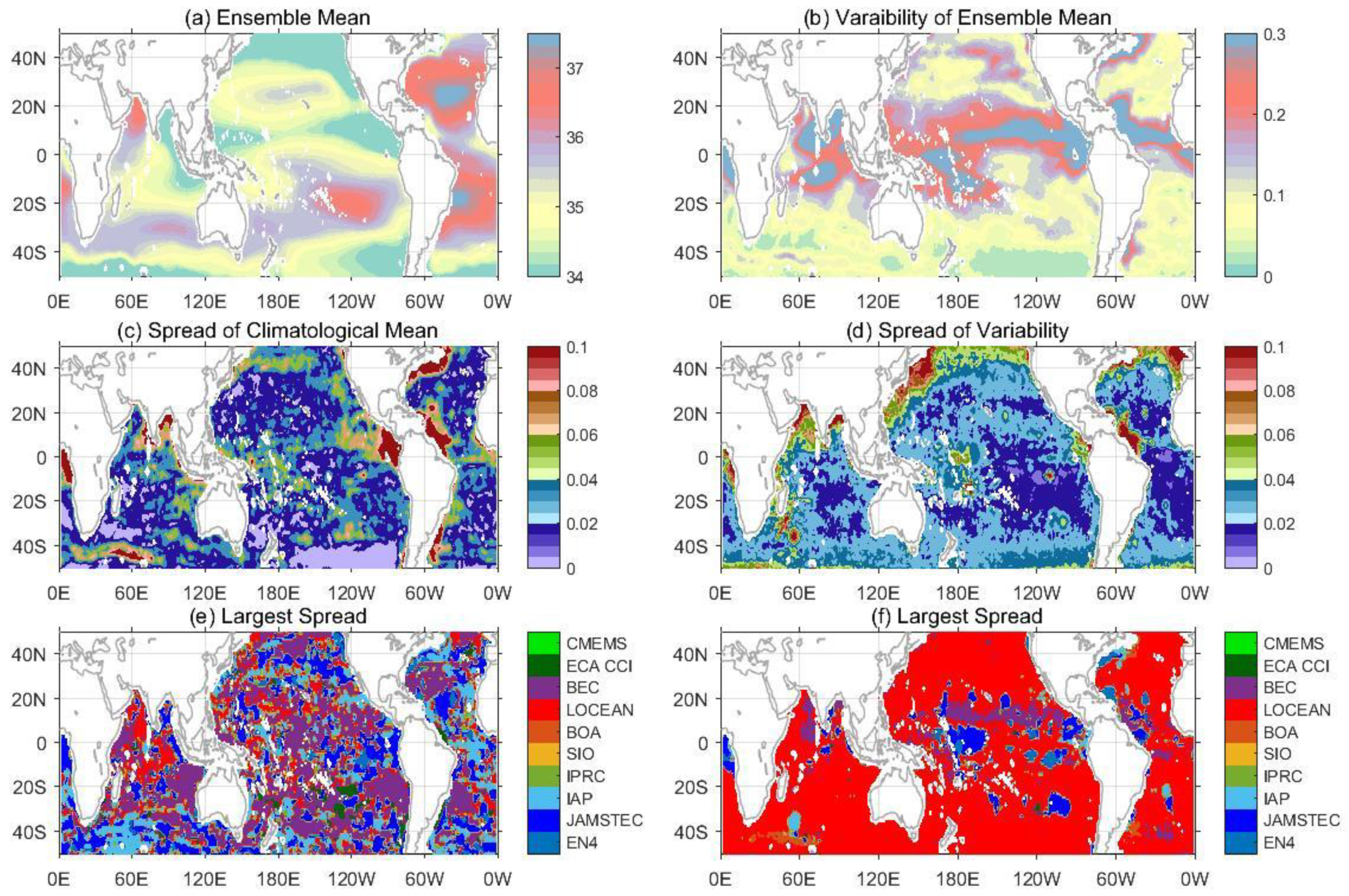
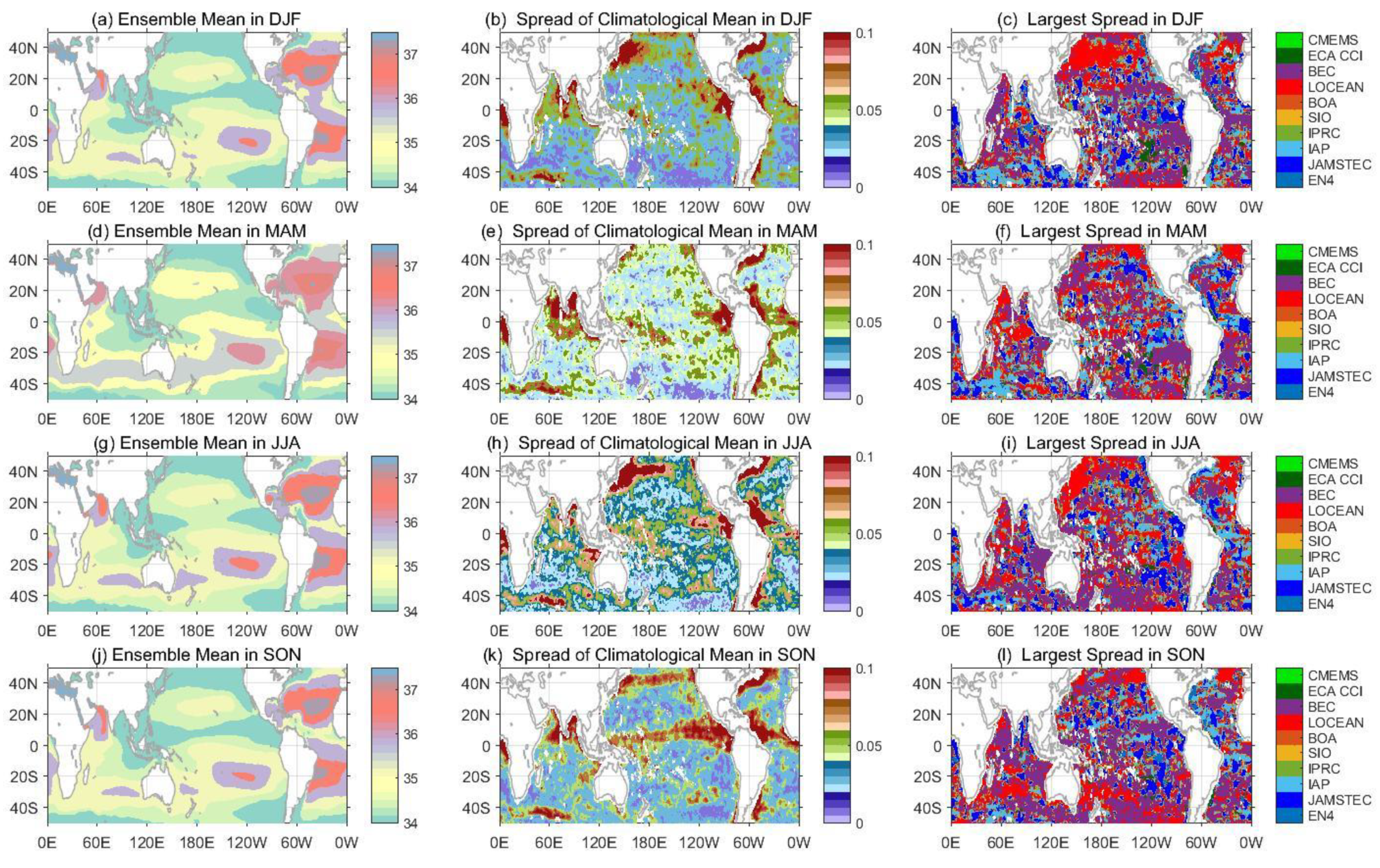
The ensemble-averaged SSS derived from ten products (Figure 1) shows an overall consistent pattern with surface freshwater fluxes [48,49]: salty surface waters mostly occur within subtropical gyres due to excessive evaporation, and fresh waters are located over tropical and subpolar regions (Figure 1a) due to overwhelming precipitation or river discharge. The SSS patterns from the ten products agree well over the open oceans, and notable differences (>0.1 g/kg, Figure 1c) occur near some coastal regions and some of the boundary currents or their extensions. JAMSTEC, BEC, IAP, and LOCEAN SSSs make larger contributions to the spread of the ensemble mean SSS over the global ocean than the SSSs from other datasets. The spread of the long-term mean SSS varies among seasons. For example, the SSS in June-July-August (JJA, Figure 1A) shows a large difference (>0.1 g/kg) over the 40~50°N region of the Pacific Ocean.
The STDs of the monthly mean SSS over 2011–2018 derived from the ensemble mean fields (Figure 1b) show the largest values (>0.3 g/kg) over the Intertropical Convergence Zone (ITCZ) and South Pacific Convergence Zone (SPCZ) regions, the Arabian Sea and the Bay of Bengal, on the southern flanks of the grand banks of Newfoundland, and in the vicinity of Rio de la Plata. Small SSS STDs (<0.05 g/kg) are mostly located over the supergyre in the Southern Hemisphere, where the variability of SSS caused by ocean dynamics and surface fluxes is small over all time scales [50]. The spread of STDs among the ten products is relatively small over the low-latitude open ocean. A large difference (>0.1 g/kg) in SSS variability occurs in the vicinity of the Kuroshio/Oyashio current and gulf streams, the northern Bay of Bengal and the Arabian Sea, the southern sections of Madagascar, and in the vicinity of the tropical Pacific Ocean. The largest spread of the SSS variability is caused by the LOCEAN SSS, which dominates the variability over most of the world (Figure 1f), indicating that it contributes most to the spread of the SSS variability between products. JASMTEC and BEC SSS cause the spread between products over the tropical Pacific.
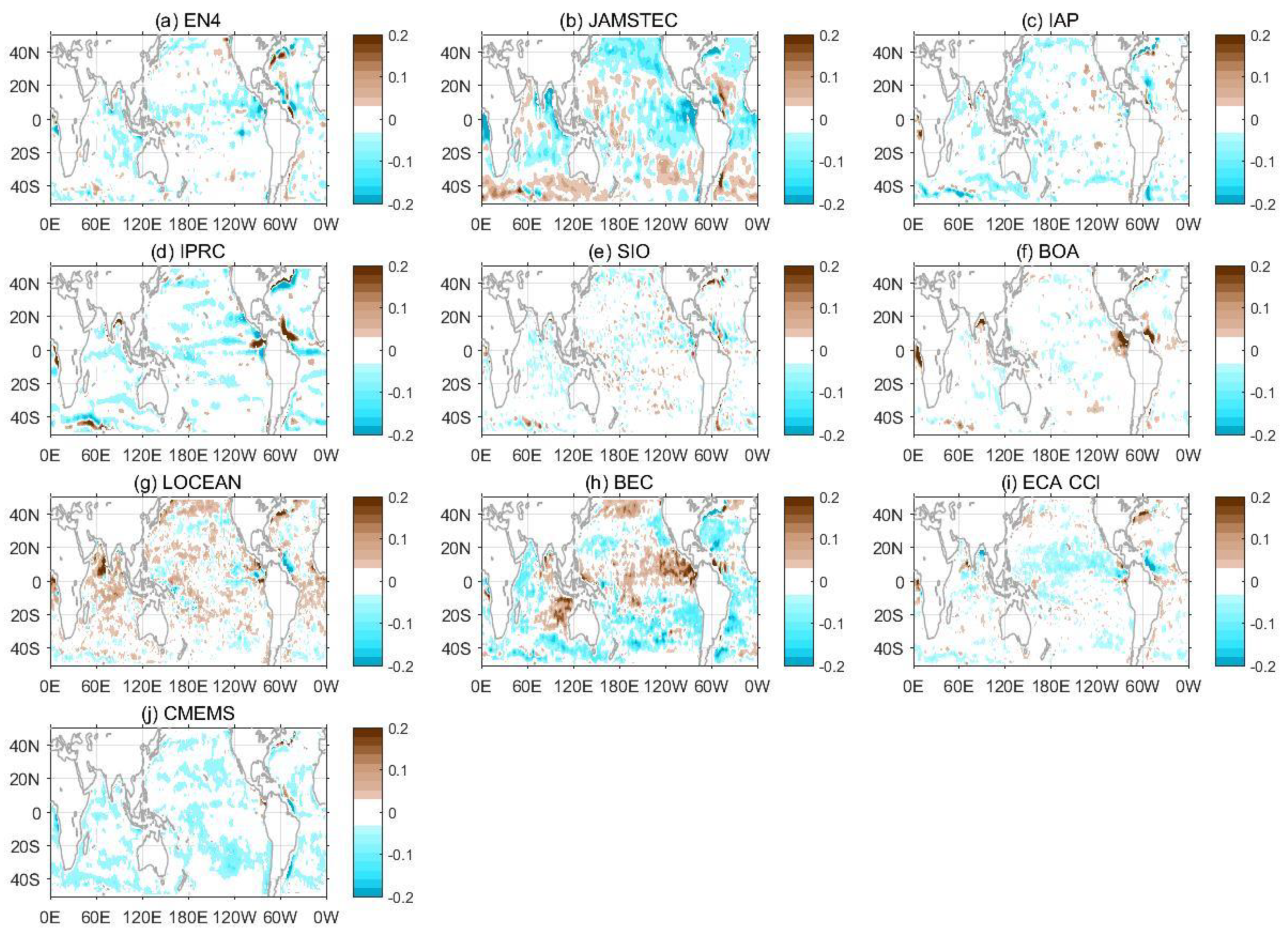
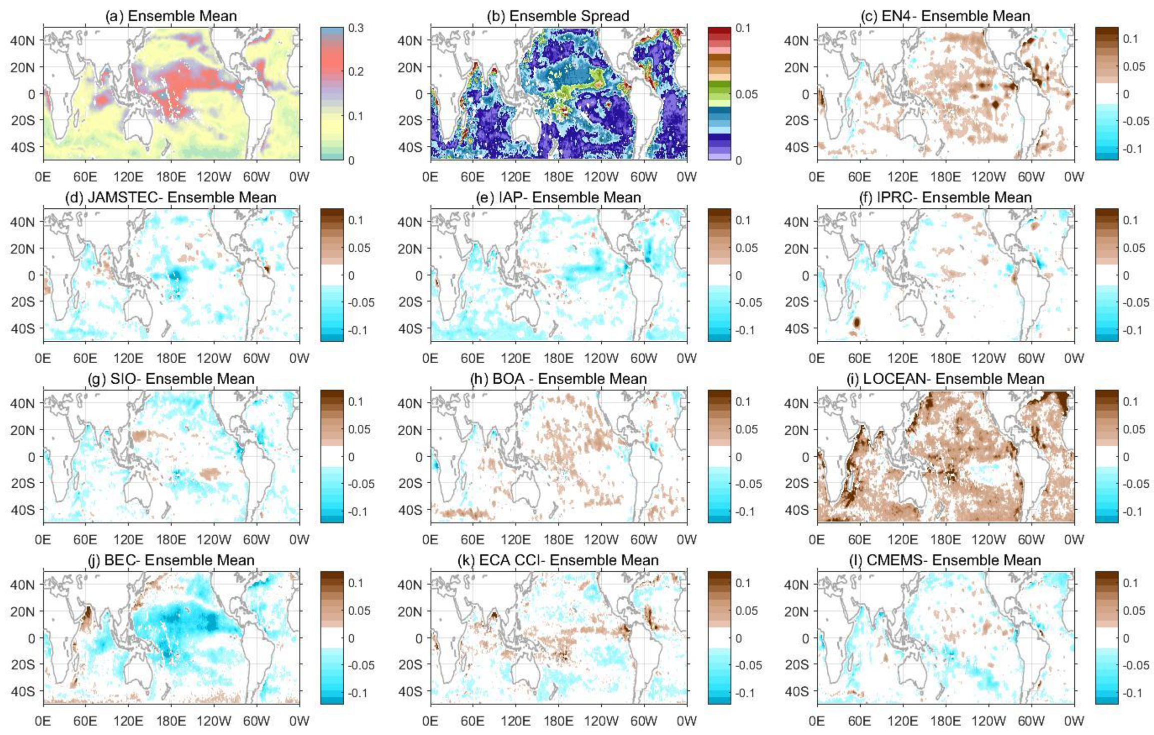
To further illustrate the difference in SSS between each product, the differences in the climatological mean and variability in the SSS between an individual product and ensemble mean fields are presented in Figure 2 and Figure 3, respectively. EN4, IAP, SIO, BOA, ECA CCI, and CMEMS show good agreement in representing the ensemble mean fields of the climatological SSS (Figure 2). The differences are generally less than 0.02 g/kg except for coastal regions and gulf streams. These localized differences are possibly related to the lack of Argo floats over the coastal region, where different underlying data sources are used to fill in data gaps in only Argo-based data products (e.g., SIO, BOA) and CTD/mooring and Argo combined data products (e.g., IAP, EN4). The JAMSTEC displays negative anomalies relative to the ensemble mean fields over most of the subtropical gyre with a magnitude of less than 0.1 g/kg. Positive anomalies (<0.2 g/kg) occur over the tropical Atlantic Ocean, the tropical Indian Ocean, and the western tropical Pacific Ocean and between 40°S and 50°S in the South Atlantic and South Indian Oceans. Anomalies in the IPRC show zonal patterns because the dynamic height model is used for the mapping method [28], in which the position of zonal currents probably influences the spatial distribution of the grid. The magnitude of the anomalies from the IPRC is greater than 0.2 g/kg near the eastern tropical Pacific Ocean, the western tropical Atlantic Ocean, and the southern side of Madagascar. The residual SSS from LOCEAN shows poor agreement with the ensemble mean SSS in the Arabian Sea, near the western tropical Atlantic Ocean, and the gulf stream. The residual SSS from BEC shows a positive sign over the tropical Pacific Ocean, the subpolar North Pacific Ocean, and the eastern tropical Indian Ocean, with magnitudes of 0.05~0.2 g/kg. Aside from these locations, the BEC is generally fresher than the ensemble mean SSS fields.
The JAMSTEC, IAP, IPRC, SIO, and CMEMS show consistent SSS variability (Figure 3). The magnitude of the residual from the ensemble mean SSS variability derived from those products is less than 0.02 g/kg. EN4, BOA and ECA CCI show strong variability in the tropical Pacific Ocean, the tropical Atlantic Ocean, the tropical Indian Ocean, from 40–45°N in the North Pacific Ocean, and from 40–50°S in the south Indian Ocean, with magnitudes between 0.02 and 0.2 g/kg. SMOS LOCEAN shows strong variability (i.e., positive sign of residuals) over most of the global ocean. The SMOS BEC shows strong variability near the Kuroshio current, in the northern Arabian Sea, and over the band of 40°S–50°S. Over the tropical oceans, the BEC generally shows weak variability.
3.2. Sub-Annual SSS Variability
The STD of the 11-month high-pass SSS time series is used here to measure the magnitude of the sub-annual variability in SSS (Figure 4). Most of the large STDs (>0.3 g/kg) are observed near the major river outlets [51]. For example, large sub-annual SSS variations are located near the Congo plume area, the Rio de la Plata Estuary, and near the Ganges, Brahmaputra/Irrawaddy and Salween Rivers. Large STDs are also observed in the eastern tropical Pacific Ocean, which is strongly impacted by rainfall. Thus, all the regions with high sub-annual SSS variability are in direct response to freshwater fluxes originating from river discharge or rainfall, highlighting the important role of freshwater fluxes in modulating the sub-annual SSS variability. Oceanic circulation also plays a role. For example, large sub-annual SSS variations are found to the north of the Amazon River mouth due to strong northward flows. Other important causes of the sub-annual SSS variations could be sub-annual changes in the wind stress. For example, Li et al. [52] reported that wind stress-forced ocean processes driven by Madden-Julian oscillations are the main driver of sub-annual SSS variability in the tropical Indo-Pacific Ocean.
Considerable differences (>0.08 g/kg) between products (Figure 4b) also occur where the STDs (Figure 4a) are relatively large (i.e., near the eastern and western tropical Atlantic Ocean or the northern Bay of Bengal). This difference is expected because these locations are mainly near the coastal region, where satellite SSS is affected by land-sea contamination [34], and only Argo-based products is biased because the number of Argo profilers is low. Thus, insufficient data sources also contribute to the large spread among datasets. Good agreement in the STDs among products occurs in the tropical and subtropical open ocean, where the spread is generally less than 0.04 g/kg.
For individual products, BOA, and ECA CCI are generally consistent with the ensemble mean sub-annual SSS variations over most of the global ocean. An exception occurs near the strong current regions in BOA, which shows a large magnitude in the SSS sub-annual variations. EN4, IAP, SIO, IPRC, and CMEMS generally show weaker sub-annual variabilities in SSSs than the ensemble mean STDs at each grid point. There are exceptions. For example, in the IPRC product, high STDs with anomalies larger than 0.1 g/kg are found on the southeastern side of Madagascar. The relationships between JAMSTEC, and BEC and the ensemble mean SSS STDs vary depending on location. JAMSTEC shows the largest STDs among the ten products near the dateline in the tropical Pacific Ocean, but small STDs occur in the subpolar region. BEC shows small STDs over the tropical ocean but large STDs in the subpolar region. LOCEAN shows stronger sub-annual SSS variability than the ensemble mean value over most of the global ocean. The largest difference (>0.1 g/kg) occurs near the eastern tropical Pacific, in the western tropical western Atlantic, in the western North Pacific, and over the subpolar gyre, and all the above locations are consistent with regions with large spreads of the STDs (Figure 4b). Therefore, LOCEAN contributes most to the spread of STDs on the sub-annual time scale.
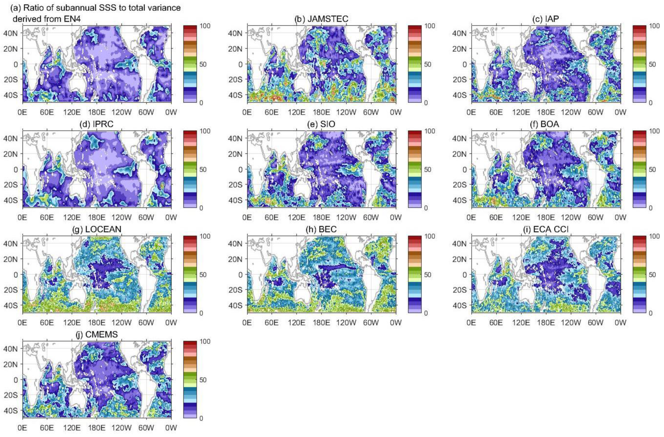
The ratio of the square of the sub-annual SSS STD to the total variance (Figure 5) is used here to assess to what degree the sub-annual SSS is representative of the total signal in each product. The contribution of sub-annual variability to the total variance is generally between 0% and 20% in EN4 and IPRC. In IAP, SIO, BOA, and CMEMS, the contribution of the sub-annual SSS to the total SSS variations is 0–20% over the tropical Pacific Ocean and 20–40% over most of the Atlantic and Indian Oceans. In JAMSTEC, LOCEAN, BEC, and ECA CCI, the contributions are 20–50% for most regions worldwide. The sub-annual SSS in LOCEAN, BEC, and ECA CCI can explain 20–60% of the variance in the SSS signal in the subtropical and subpolar gyres and 0–20% in the tropical Pacific Ocean and the tropical Indian Ocean. Thus, all ten products show a consistent pattern over the tropical Indian and tropical Pacific Oceans, in which the sub-annual variability accounts for only 0~20% of the total variance. The largest contribution made by the sub-annual signal to the total SSS variance is generally observed from satellite data rather than in situ-based data, which is due to the low temporal sampling resolution of in situ observations. However, this difference is not always the case. For example, for JAMSTEC, most of the grid points in the section poleward of 20°S sometimes show larger contributions to the total variance made by sub-annual SSS than those from LOCEAN and BEC. These regions with a high percentage of sub-annual SSSs compared with the total variances (Figure 5b) are generally associated with high STDs (Figure 4d) in JAMSTEC.
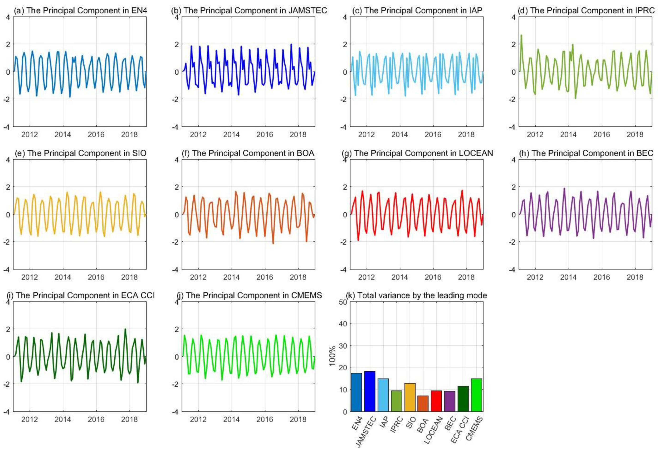
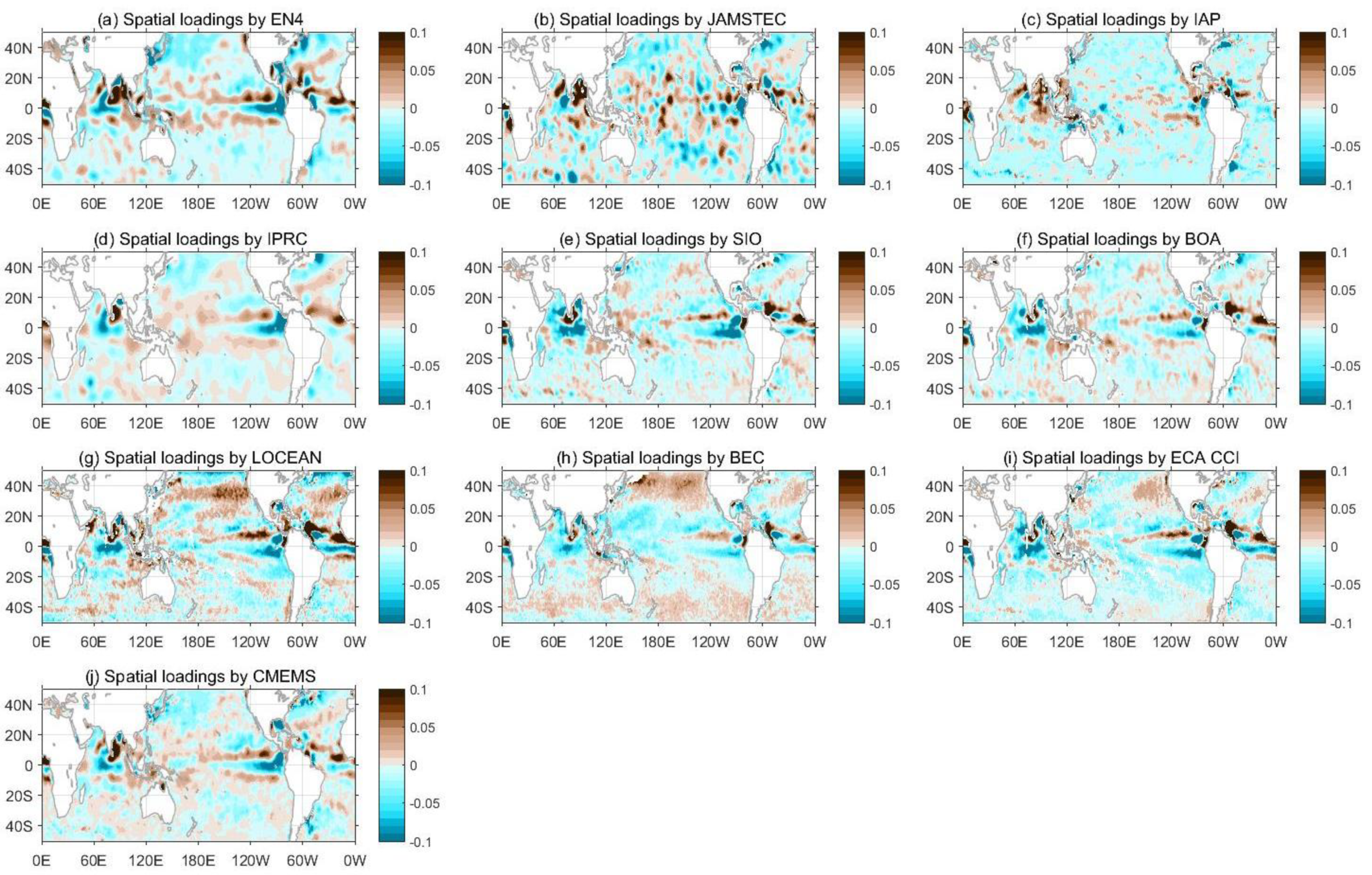
To further explore the characteristics of the sub-annual SSS variability over the globe, an EOF is performed for the ten products. There are two cycles in one year in for most of the products (Figure 6), indicating that the semiannual cycle is the leading mode of the sub-annual SSS variances. However, the two cycles in one year show different amplitude, indicating an higher frequency variability contributes to the first mode of the sub-annual SSS. The exceptions are the EN4 (Figure 6b) and IAP (Figure 6c). The EN4 shows one dominant peak and two troughs in one year, and IAP shows multiple peaks and troughs in one year. EN4, IPRC, SIO, BOA, LOCEAN, BEC, ECA CCI, and CMEMS show similar spatial patterns of the first mode by EOF over the tropical oceans (Figure 7). In IAP, negative anomalies spread over extratropical oceans. The first leading mode can account for less than 20% of the total sub-annual SSS variance from each product (Figure 6k), with the largest contribution found in IAP (18%). As mentioned above, the differences in the temporal and spatial patterns of the first leading modes for the sub-annual SSS between products are possibly attributed to the differences among products, including temporal sampling, underlying data, and mapping methods.
3.3. The Annual Cycle of SSS
The STDs of the estimated annual harmonics (Figure 8a) in the ensemble mean fields show the regions with large seasonal variations (>0.3 g/kg) in the ITCZ and SPCZ and strong salinity gradient regions (Figure 2 from Yu [48]), including the eastern Arabian Sea, the western and northern Bay of Bengal, the central tropical Indian Ocean, the eastern side of Japan, and the western coast of the North Atlantic. The results are consistent with those from Bingham et al. [53], which were derived from in situ profiles before 2010, and agree with the results from Yu et al. [54], which were derived from 4 satellite products and two gridded in situ datasets from 2016 to 2018. The seasonal SSS variability in the tropical ocean is dominated by evaporation-minus-precipitation (EMP), especially precipitation [53]. Ocean dynamics, including horizontal advection and diffusion, play an important role in the establishment of the seasonality of surface salinity over extratropical regions [50].
The regions of the pronounced SSS annual cycle are also regions of large spread from the ensemble mean (>0.05 g/kg). The maximum spread (>0.1 g/kg) occurs over the eastern Arabian Sea, the northern Bay of Bengal, to the eastern side of Japan, the eastern tropical Pacific, along the gulf streams, the western tropical Atlantic, and the western subtropical South Atlantic (near 40°S). Most of the regions in which the largest spread occurs are caused by strong annual SSS variability from LOCEAN (especially at tropical Atlantic and North Pacific). Exceptions include the eastern tropical Pacific Ocean, the western tropical South Pacific Ocean, the subpolar gyres of the North Pacific and South Indian Oceans, the eastern Arabian Sea, and along the gulf streams, where LOCEAN shows a weak annual cycle. The BEC shows the smallest variances over most of the subtropical and tropical oceans among the ten products. Hence, a major difference in annual SSS variability exists between the two SMOS-based satellite SSSs. This finding indicates that the annual SSS variability in satellite SSS data is highly dependent on the difference between bias correction methods. The ECA CCI shows a larger annual variance than the ensemble mean over the tropical ocean. The horizontal distribution of the annual cycle of SIO, CMEMS and BOA SSS generally agrees well with that of the ensemble mean with a difference smaller than 0.02 g/kg over most of the global ocean. Relatively large STDs (between 0.02 and 0.1 g/kg) are found in EN4, JAMSTEC, and IPRC over tropical oceans.
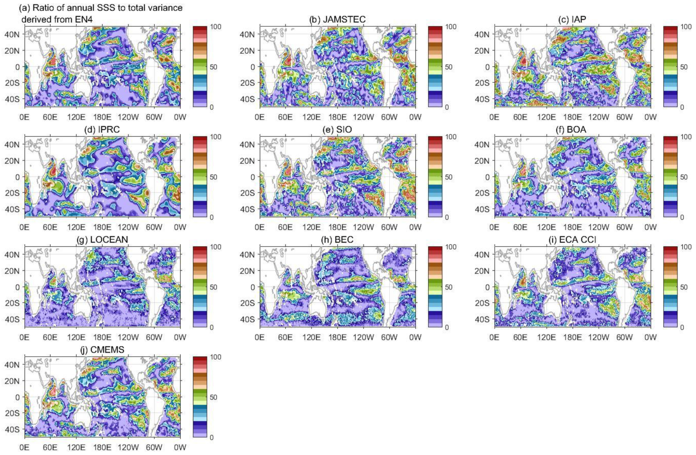
The contribution of the annual SSS variance to the total variance (Figure 9) for most of the SSS products is relatively small, with a magnitude of 0~0.4 over most of the Pacific Ocean. A large ratio of annual SSS variation to the total variance (>60%) occurs over the Arabian Sea, the western tropical Indian Ocean, in the vicinity of the Kuroshio extension, over the eastern tropical and subtropical South Pacific, the eastern subtropical North Atlantic, the tropical Atlantic Ocean, and the central/eastern subtropical South Atlantic. Our results show a smaller percentage of the total variance than those shown in Yu et al. [54]. Yu et al.’s results are based on a short period from 2016 to 2018, while our coverages are from 2011 to 2018. Thus, the difference could be due to a difference in the low-frequency variability, which is not present in Yu et al.’s result, or a difference in the magnitude of high-frequency variability between before 2016 and after 2016.
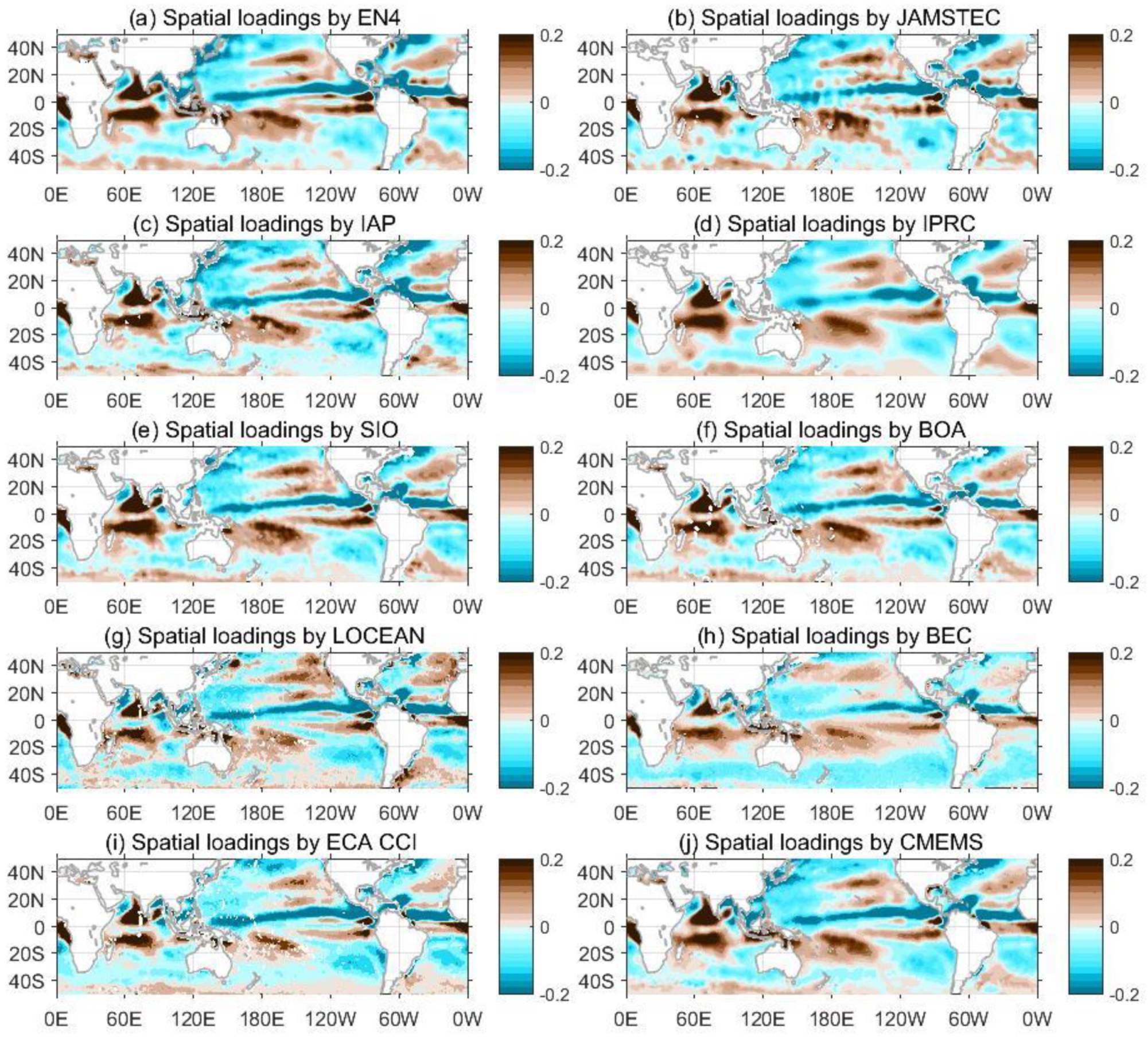
The leading spatial loadings and their principal components derived from the annual SSS time series show consistency among the ten products (Figure 10, and Appendix A Figure A2). The times series of the principal components derived from individual product are aligned with each other (Figure 10a). The maximum SSS occurs in September for the ten SSS products, and the minimum SSS occurs in March for all products. The principal components account for 55~75% of the seasonality. The results are consistent with those from Boyer and Levitus [55] and Bingham et al. [53]. The spatial loadings for the leading annual SSS mode derived from individual products are consistent with each other (Figure A2). The ensemble mean of spatial loading for the leading annual SSS mode shows that positive anomalies generally occur over the central and eastern North Pacific and North Atlantic Oceans, the central to eastern tropical South Pacific and South Atlantic Oceans, the western tropical South Pacific Ocean, the central and western tropical Indian Ocean, and the eastern Arabian Sea. Negative anomalies occur elsewhere.
3.4. Interannual Variability in SSS
The maximum in the interannual SSS variability (>0.2 g/kg) from the ensemble mean fields occurs over the tropical Pacific Ocean, the northeastern North Pacific Ocean, the northern Bay of Bengal, the eastern tropical Indian Ocean, and the western tropical Atlantic Ocean (Figure 11). The large interannual SSS variability in the tropical Indian Ocean and the northern Bay of Bengal can be attributed to the Indian Ocean dipole [56,57,58]. The interannual SSS variations over the tropical Atlantic and Pacific are caused by the interannual meridional displacements of the ITCZ [59], which are probably associated with ENSO in the Pacific Ocean [60] or the Atlantic Meridional Dipole in the Atlantic. In the eastern tropical South Atlantic Ocean and the northeastern North Pacific Ocean, relatively strong interannual variabilities with magnitudes of 0.15 g/kg~0.25 g/kg are observed. The SSS variations are attributed to changes in the discharge of the Congo River [61]. The cause of the interannual SSS variability in the northeastern North Pacific Ocean is probably associated with changes in the ocean dynamic processes (Figure 2 from [50]), but the key force is still an open question. Over other regions, the interannual SSS variability is generally between 0 and 0.1 g/kg.
The largest spread (>0.06 g/kg) occurs over the tropical Pacific Ocean (Figure 11b), the northern Bay of Bengal and the Arabian Sea, to the north of the Amazon River plume, over the eastern subpolar gyre in the North Atlantic Ocean and to the southeastern section of Madagascar (60°E and 40°S). The JAMSTEC, IAP, IPRC, SIO, BOA, ECA CCI, and CMEMS show consistent interannual variations with the ensemble mean over most of the global ocean. The large spread in the interannual SSS variations mainly results from two SMOS satellite-based products. The interannual SSS variability from LOCEAN displays large variances over most of the global ocean, and BEC displays a smaller variance than the ensemble means in the tropical Pacific Ocean.
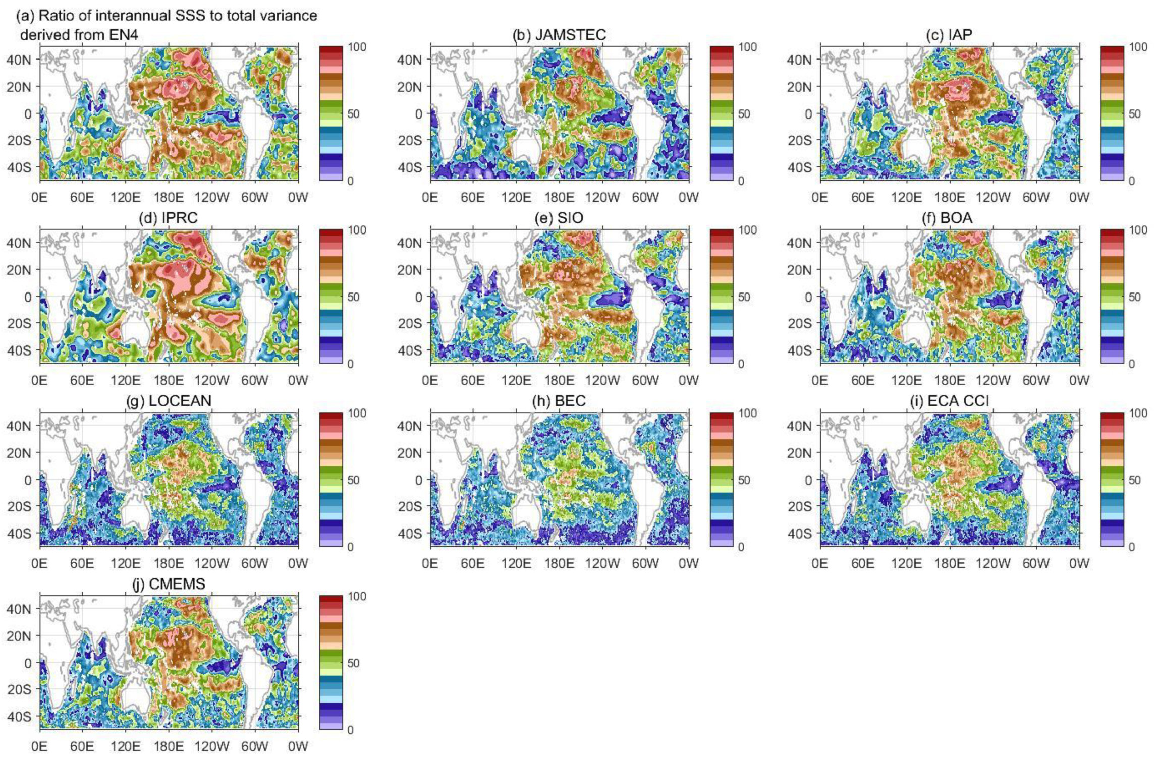
The regions with large interannual SSS variability also make a large contribution to the total SSS variance (Figure 12). The regions in which the interannual SSS accounts for over 60% of the total variance are in most of the Pacific Ocean and the northeastern Atlantic Ocean. The ratio of interannual SSS to the total SSS variance from in situ-based products (40~90%) is generally larger than those observed from only satellite-based products (20~80% for LOCEAN, BEC, and ECA CCI) over most of the Pacific Ocean. This result could be partially explained by the larger high-frequency variability observed from satellite data than those observed from in situ-based products (Figure 5), which leads to a small contribution of the low-frequency variances to the total variance.
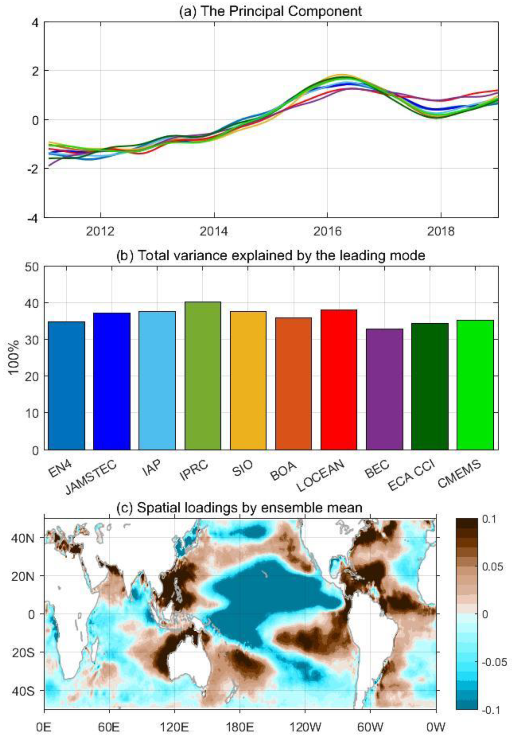
The first leading (Figure 13) mode can generally account for approximately 33% to 40% of the total interannual SSS variability. The time series of the first leading mode of the interannual SSS shows consistent variations in ten products: a steady increase from 2011 to 2016 followed by a sharp decrease from 2016 to 2018 (Figure 13a). These changes are consistent with the ENSO signal, in which extremely strong El Niño events occurred in 2015–2016 and La Niña events occurred in 2018–2019. The spatial distribution of the first mode shows consistent variations among the ten products (Figure 3A). The spatial pattern of the first mode of the interannual SSS derived from the ensemble mean in the Pacific shows horseshoe-like patterns in the tropical Pacific Ocean: positive anomalies stretch from the west coast to the northeast/southwest in the Northern/Southern hemisphere (Figure 13c). Positive anomalies are also found over the northeastern North Pacific Ocean, the eastern South Pacific Ocean, the eastern Indian Ocean, the tropical Atlantic Ocean, and the western subtropical South/North Atlantic Ocean. SSS shows contrasting variations between the eastern and western Maritime Continent (MC), which is probably associated with a change in the Walker circulation [62].
3.5. The Dominant SSS Signal
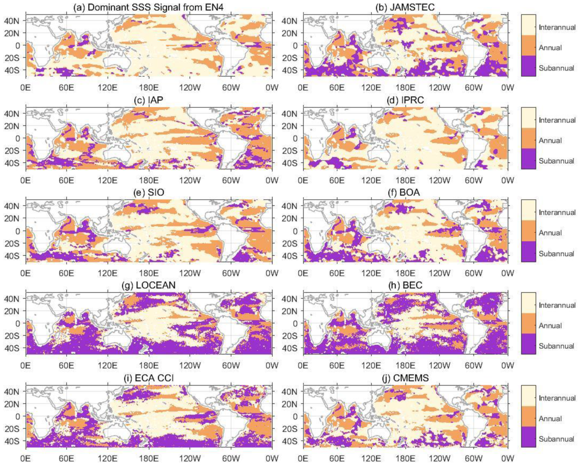
This section evaluates the largest SSS STDs among different time scales for ten products over the global ocean (Figure 14). We emphasize that this section compares SSS STDS over the 2011–2018. Results will change if a different period is chosen, For EN4, JASMTEC, IAP, IPRC, SIO, BOA, and CMEMS SSS products, the interannual and annual SSSs play the dominant roles over most of the global oceans. Over most of the Pacific Ocean, the interannual SSS plays the dominant role in the total variances. In the northwestern North Pacific, the eastern South Pacific, under the ITCZ, and some regions in the tropical Indian Ocean, the SSS variability is dominated by the annual signal. In the Atlantic Ocean, the annual SSS shows a larger horizontal extent than others on different time scales for EN4, JASMTEC, IAP, IPRC, SIO, BOA, and CMEMS. The dominance in total variances from sub-annual SSS are mostly found on the southern side of 30°S, some places in the Bay of Bengal, and subpolar North Atlantic and North Pacific Ocean for EN4, JASMTEC, IAP, IPRC, SIO, BOA, and CMEMS.
For only satellite-based SSS products (LOCEAN, BEC, and ECA CCI), the sub-annual SSS displays a wider horizontal extent in SSS variance than the other products. For LOCEAN and BEC, the sub-annual SSS variability plays the leading role over the high latitude regions in the Southern Hemisphere, the northern subpolar gyre in the North Pacific Ocean, and the central and western North Atlantic Oceans. Over the western tropical Pacific Ocean, the interannual SSS variabilities from LOCEAN, BEC, and ECA CCI play the leading role, agreeing with the results from EN4, JASMTEC, IAP, IPRC, SIO, BOA, and CMEMS (Figure 14). Over some areas in the eastern tropical and subtropical South Pacific Ocean and the tropical Indian and Atlantic (excluding regions near 0°S) Oceans, the annual SSS plays the primary role in the SSS variance, which is also consistent with the results from the other products in Figure 14.
3.6. The Statistical Summary
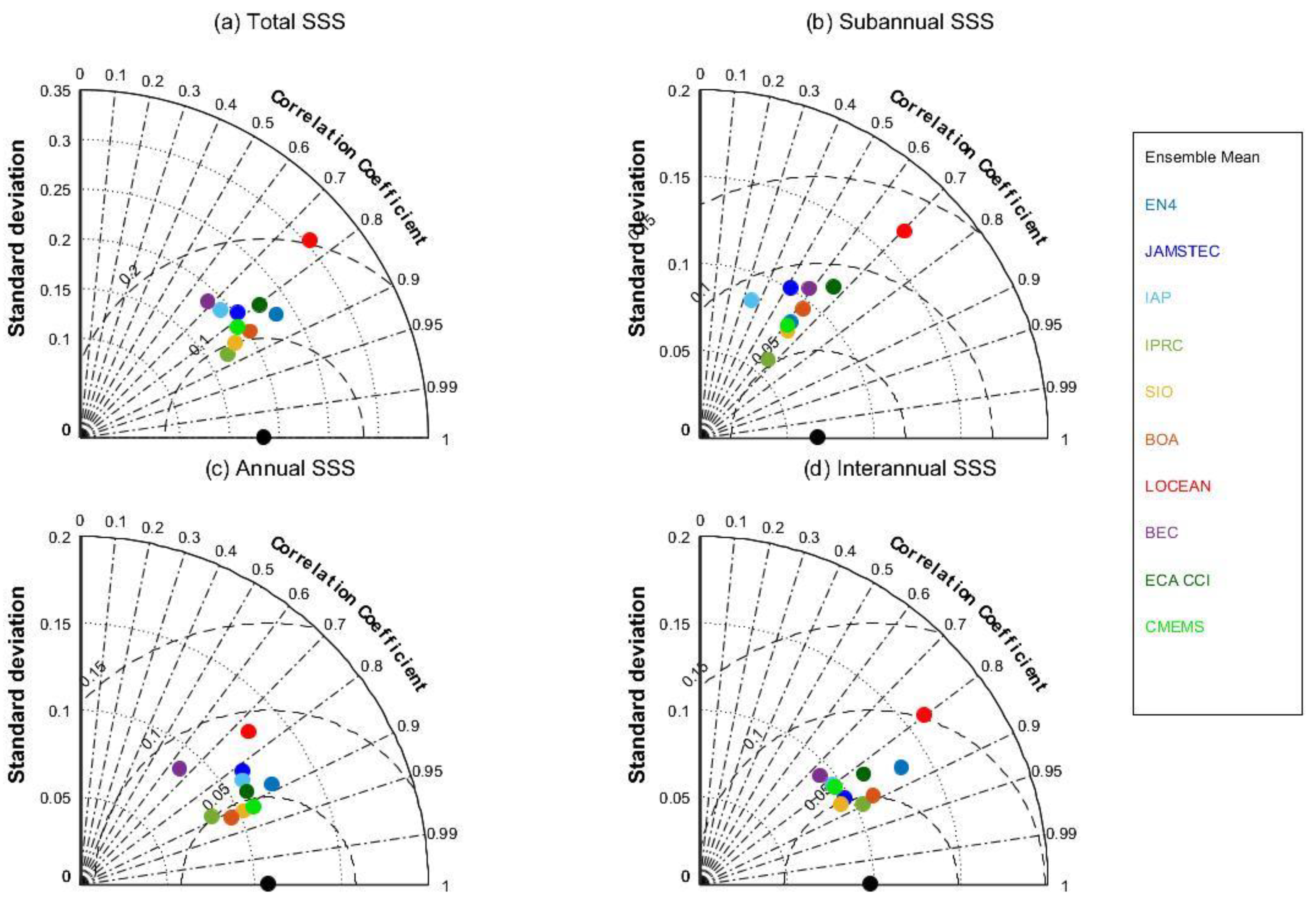
Based on the previous analysis, we summarize the intercomparison of SSS products using a Taylor diagram (Figure 15). The global mean ECA CCI SSS maps most closely resemble the ensemble mean fields on the original, sub-annual, and interannual time scales. On the annual time scale, SIO, BOA, and CMEMS show a better match with the ensemble mean fields than the other products. On all of the time scales, the global mean SSS variations from LOCEAN show the smallest resemblance with those from the ensemble mean fields.
The global mean STD of the ensemble mean SSS variations is 0.18 g/kg (Figure 15a). LOCEAN shows larger global mean STDs than the other products on most of the time scales, except for the annual cycle. The global mean total SSS variations from LOCEAN are over 0.3 g/kg, and those from the other products are between 0.15 and 0.25 g/kg. The largest STD of the decomposed SSS signal for the ensemble mean over the period between 2011 and 2018 occurs on the annual time scale (Figure 15c), with a magnitude of 0.11 g/kg. The global mean STD of the interannual SSS for the ensemble mean is 0.1 g/kg, and the STD of the sub-annual variability is 0.07 g/kg. At subannual, annual and interannual time scales, the STDs of SSS variations from most of the products (except for LOCEAN) are generally between 0.05 and 0.15 g/kg.
The correlation coefficients for the sub-annual time scale between each product and ensemble mean are generally small, with magnitudes of 0.3~0.7 (satisfying the 90% confidence level). On the annual time scale, the correlation coefficients are significant, and the magnitude is between 0.6 and 0.95. On the interannual time scale, the correlation coefficients are between 0.7 and 0.9, also satisfying the 90% confidence level. Therefore, the annual and interannual SSS variations are more consistent among products than the sub-annual SSS variations. Thus, the patterns of the sub-annual SSS variations are more likely to vary depending on different products.
4. Discussion
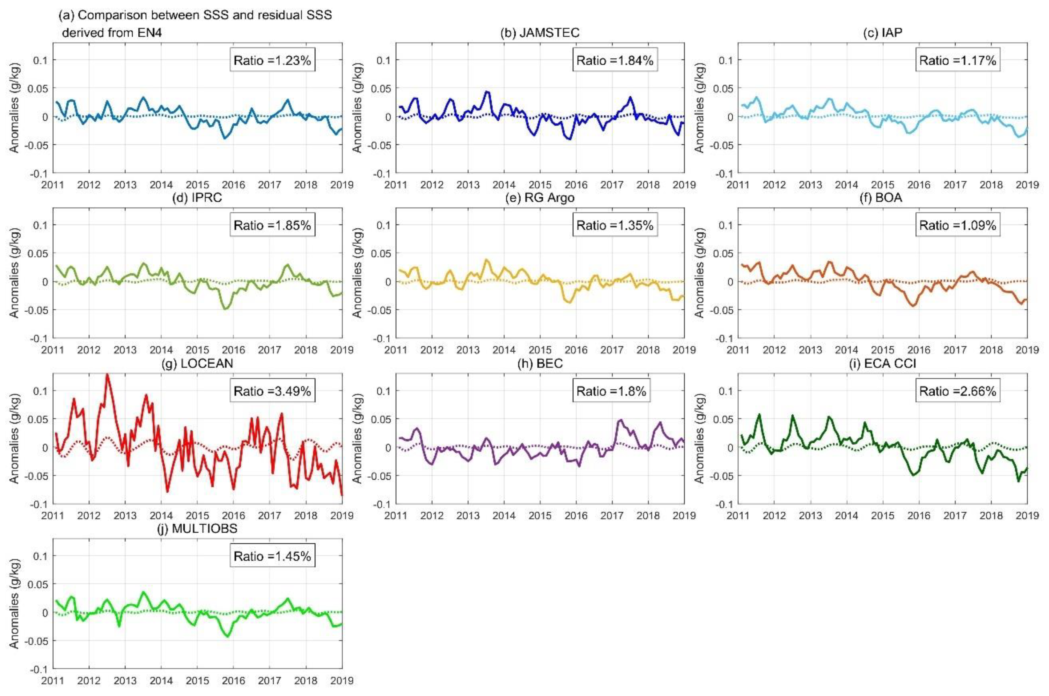
In this analysis, the time series of SSS is decomposed into three components. To evaluate the performance of the decomposition, we analyze the residuals derived from subtracting the time series of SSS from the sum of the sub-annual, annual and interannual signals. We use the ratio of the residual variation to the total SSS variance as a measurement of the uncertainty due to the decomposition in our analysis. From the global mean SSS perspective, the residual SSS accounts for less than 4% of the total variance (Figure A4). At each grid point over the global ocean, the ratio of the residual SSS variance to the total SSS variance is generally less than 10% (Figure A5). Thus, the residual is small compared to the original signal, and our methods of decomposition can capture most of the SSS variance.
This analysis applies the 12th-order Hanning filter to SSS data to derive variations on different time scales. The same filter has also been applied in the eastern tropical Pacific to derive spatial patterns in SSS variability [63]. Other filters, such as Butterworth, are also commonly used in research on SSS changes. For example, Subrahmanyam et al. [64] and Trott et al. [65] applied the fourth Butterworth filter to SSS in the Bay of Bengal to analyze the high-frequency SSS variability. Hasson et al. [66] applied the fourth Butterworth filter to SSS to analyze the link between SSS variability and mesoscale eddies. The running mean is also broadly applied in the analysis to derive low-frequency variability [28]. For example, an 18-month running mean was applied by Durack and Wijffels [3] to analyze the decadal variability in SSS over the globe. To assess the sensitivity of our results to the different methods applied, we calculate the STDs of SSS from the ensemble mean on different time scales (Table 2). We use the 12th-order Hanning/Butterworth filter to calculate the SSS variability on different time scales. For the comparison of the low-frequency SSS variability, we also calculate the STD by using the 13-month running mean. The SSS variabilities on different time scales by different methods agree with each other. The temporal coverage in this analysis is relatively short. To assess the method reliability of the temporal coverage, we also apply the EOF method to the SSS over the 2005–2018 from EN4, JAMSTEC, IAP, IPRC, SIO, and BOA. We find consistent spatial and temporal patterns of the leading mode on three different time scale with results in the previous section. Thus, the derivations of SSS variabilities on different time scales are robust. Furthermore, the salinity at 10m from EN4, JAMSTEC, IAP, IPRC, SIO, and BOA are also examined in this analysis. The temporal and spatial variabilities of dominant mode of salinity on sub-annual, annual and interannual time scales show consistent results with salinity at 0m. Hence, results here will not change if 10m from in situ-based products are used.
Notably, the results in this analysis are sensitive to the calculation procedures. This analysis derives the SSS variations by subtracting the annual cycle of SSS as the first step and applying the filters to as the second step. If the first step is eliminated and only the second step is applied to the series to derive the high/low-frequency variability, there would be some signal leaked from the annual cycle, which would contaminate the results.
Although multiple efforts have been made in previous research to increase the representation of the spatiotemporal variability in the SSS, a large discrepancy still exists among different products. The difference could be caused by the differences in sampling [21,22] and mapping methods [29] and systematic errors when retrieving salinity data [24,34]. The possibility of identifying the “true value” of the SSS fields is low due to the large discrepancy among products over certain regions. Further effort should be made to improve the estimation of the observed SSS variations. Such efforts should include salinity budget analysis using satellite-based variables on multiple time scales, identification of the difference in skin SSS and near-surface SSS over the global ocean, and a comprehensive analysis combining satellite retrieval and in situ-based analysis.
5. Conclusions
In this study, we provide a comprehensive and detailed intercomparison of SSS variability on multiple time scales between ten SSS products over 2011–2018. First, we calculate the STDs of the total SSS variations over 2011–2018 from the ensemble mean fields and each product. By comparison of individual products to the ensemble mean SSS maps, we found that the global mean ECA CCI SSS maps show the best resemblance to the ensemble mean fields on the sub-annual and interannual time scales. On the annual time scale, SIO, LOCEAN, and CMEMS show a better match with the ensemble mean fields than the other products. The global mean SSS variations from LOCEAN show the least resemblance with the ensemble mean fields at all frequencies.
Details of the findings on each time scale are summarized as follows.
On the sub-annual time scale, STDs from LOCEAN show larger values than the ensemble means over most of the global ocean. The sub-annual variability can generally explain 0~40% of the total variance over most of the global ocean among the ten products. JAMSTEC, LOCEAN, BEC, and ECA CCI generally show a higher percentage of sub-annual variability in the total variances than those in the six other products. The leading mode of the sub-annual SSS signal from most of the products is the semiannual mode, which shows two peaks/troughs in one year. However, the leading mode can account for less than 20% of the total sub-annual variances for all products, indicating that other variances also play a role in regulating the sub-annual SSS.
The uncertainties in the annual cycle of SSS among the ten products are mainly associated with the two SMOS-based products. LOCEAN shows stronger variability than the ensemble mean fields over most of the tropical Atlantic and North Pacific, and BEC shows weaker variability than the ensemble means over subtropical and tropical oceans. Most SSS products show a ratio of the annual SSS variance to the total variance with a magnitude of 0~0.4 over the Pacific Ocean. However, in other ocean basins, a ratio of >0.6 is observed in most of the products. The temporal and spatial distributions of the leading mode for the annual SSS show consistency among the ten products. The maximum SSS occurs in September, and the minimum SSS occurs in March for the leading mode.
The percentage of interannual changes to the total SSS variance is larger from in situ-based products (40~90%) than those observed from only satellite-based products (20~80%, LOCEAN, BEC, and ECA CCI). Good agreement in the temporospatial variability in the dominant mode for interannual SSS is reached among the ten products.
In summary, our results offer a detailed intercomparison of the variability on different time scales from ten products. High correlation coefficients (0.6~0.95) are found in the global mean annual and interannual SSSs between individual products and the ensemble mean. Furthermore, this study shows good agreement among the ten datasets in representing the dominant mode of SSS on the annual and interannual time scales. The results enhance our confidence in using in situ-based and satellite-based SSS products for low-frequency and climate-related research.
Author Contributions
Both authors H.L. and Z.W. contributed equally to all aspects of this study and the writing of this manuscript. All authors have read and agreed to the published version of the manuscript.
Funding
This research was funded by the National Key Research and Development Program of China (No. 2017YFC1404201), the National Natural Science Foundation of China (42006005, 41821004), the Postdoctoral Innovation Research Program of Shandong Province (SDSBSH202002), and the Qingdao Postdoctoral Applied Research Project (QDBSH202004).
Institutional Review Board Statement
Not applicable.
Informed Consent Statement
Not applicable.
Data Availability Statement
The ten SSS data presented in this study are openly and freely available. EN4 is available at https://www.metoffice.gov.uk/hadobs/en4/en4-0-2-data-sources.html (accessed on 20 February 2021), JASMTEC is available at http://www.jamstec.go.jp/ARGO/argo_web/argo/?page_id=83&lang=en (accessed on 20 February 2021), IAP is available at http://159.226.119.60/cheng (accessed on 20 February 2021), IPRC is available at http://apdrc.soest.hawaii.edu/projects/argo/ (accessed on 20 February 2021), SIO is available at http://sio-argo.ucsd.edu/RG_Climatology.html (accessed on 20 February 2021), and BOA is available at http://www.argo.org.cn/ (accessed on 20 February 2021). The SMOS SSS data produced by the LOCEAN/IPSL (UMR CNRS/UPMC/IRD/MNHN) la-boratory and ACRI-st company is available at http://www.catds.fr/ (accessed on 20 February 2021) [http://0-doi-org.brum.beds.ac.uk/10.17882/52804#69293 (accessed on 20 February 2021)] and the SMOS SSS produced from BEC is available at http://bec.icm.csic.es/bec-ftp-service/ (accessed on 20 February 2021). The ECA CCI SSS is available at https://climate.esa.int/en/projects/sea-surface-salinity/data/ (accessed on 20 February 2021) [DOI:10.5285/9ef0ebf847564c2eabe62cac4899ec41]. The CMEMS is available at https://resources.marine.copernicus.eu (accessed on 20 February 2021).
Acknowledgments
We appreciate access to all the freely available products that made this study possible. These products include gridded salinity products from EN4, JASMTEC, IAP, IPRC, SIO, and BOA. The satellite SSS data includes products released by the LOCEAN/IPSL (UMR CNRS/UPMC/IRD/MNHN) laboratory and ACRI-st company, the Barcelona Expert Center, the ESA climate office, and the E.U. Copernicus Marine Service Information.
Conflicts of Interest
The authors declare that they have no conflicts of interest.
Appendix A
Figure A1.
The horizontal distribution of the (a,d,g,j) ensemble means, (b,e,h,k) STD, and (c,f,i,l) largest spread of seasonal SSS derived from ten products averaged over 2011–2018.
Figure A1.
The horizontal distribution of the (a,d,g,j) ensemble means, (b,e,h,k) STD, and (c,f,i,l) largest spread of seasonal SSS derived from ten products averaged over 2011–2018.

Figure A2.
The spatial pattern of the leading mode of the annual SSS variations from ten products. The units are in g/kg.
Figure A2.
The spatial pattern of the leading mode of the annual SSS variations from ten products. The units are in g/kg.

Figure A3.
The spatial pattern of the leading mode of the interannual SSS variations from ten products. The units are in g/kg.
Figure A3.
The spatial pattern of the leading mode of the interannual SSS variations from ten products. The units are in g/kg.

Figure A4.
Time series of global mean SSS anomalies (solid lines) and the residual of the decomposed SSS signal (dotted lines) derived from ten SSS products. The ratio of the residual SSS variance to the total SSS variance is listed in the northeastern corner of each plot. The units for SSS anomalies are g/kg.

Figure A5.
The ratio of residual SSS variance to the total SSS variance in ten products. The residual SSS is derived from the subtraction of the original SSS signal from the sum of sub-annual, annual and interannual SSS time series. The units are %.
Figure A5.
The ratio of residual SSS variance to the total SSS variance in ten products. The residual SSS is derived from the subtraction of the original SSS signal from the sum of sub-annual, annual and interannual SSS time series. The units are %.

References
- Schmitt, R. Salinity and the Global Water Cycle. Oceanography 2008, 21, 12. [Google Scholar] [CrossRef]
- Helm, K.P.; Bindoff, N.L.; Church, J.A. Changes in the global hydrological-cycle inferred from ocean salinity. Geophys. Res. Lett. 2010, 37, 37. [Google Scholar] [CrossRef]
- Durack, P.J.; Wijffels, S.E. Fifty-year trends in global ocean salinities and their relationship to broad-scale warming. J. Clim. 2010, 23, 4342–4362. [Google Scholar] [CrossRef]
- Skliris, N.; Marsh, R.; Josey, S.A.; Good, S.A.; Liu, C.; Allan, R.P. Salinity changes in the World Ocean since 1950 in relation to changing surface freshwater fluxes. Clim. Dyn. 2014, 43, 709–736. [Google Scholar] [CrossRef]
- Wang, G.; Cheng, L.; Boyer, T.P.; Li, C. Halosteric Sea Level Changes during the Argo Era. Water 2017, 9, 484. [Google Scholar] [CrossRef]
- Lee, T.; Lagerloef, G.; Gierach, M.M.; Kao, H.Y.; Yueh, S.; Dohan, K. Aquarius reveals salinity structure of tropical instability waves. Geophys. Res. Lett. 2012, 39, 39. [Google Scholar] [CrossRef]
- Yin, X.; Boutin, J.; Reverdin, G.; Lee, T.; Arnault, S.; Martin, N. SMOS S ea S urface S alinity signals of tropical instability waves. J. Geophys. Res. Oceans 2014, 119, 7811–7826. [Google Scholar] [CrossRef] [Green Version]
- Menezes, V.V.; Vianna, M.L.; Phillips, H.E. Aquarius sea surface salinity in the South Indian Ocean: Revealing annual-period planetary waves. J. Geophys. Res. Oceans 2014, 119, 3883–3908. [Google Scholar] [CrossRef]
- Delcroix, T. Observed surface oceanic and atmospheric variability in the tropical Pacific at seasonal and ENSO timescales: A tentative overview. J. Geophys. Res. Oceans 1998, 103, 18611–18633. [Google Scholar] [CrossRef]
- Ballabrera-poy, J.; Murtugudde, R.; Busalacchi, A.J. On the potential impact of sea surface salinity observations on ENSO predictions. J. Geophys. Res. 2002, 107, 8007. [Google Scholar] [CrossRef]
- Maes, C.; Picaut, J.; Belamari, S. Salinity barrier layer and onset of El Nino in a Pacific coupled model. Geophys. Res. Lett. 2002, 29, 59. [Google Scholar] [CrossRef]
- Zhu, J.; Huang, B.; Zhang, R.-H.; Hu, Z.-Z.; Kumar, A.; Balmaseda, M.A.; Marx, L.; Kinter III, J.L. Salinity anomaly as a trigger for ENSO events. Sci. Rep. 2014, 4, 6821. [Google Scholar] [CrossRef] [PubMed] [Green Version]
- Qu, T.; Yu, J.-Y. ENSO indices from sea surface salinity observed by Aquarius and Argo. J. Oceanogr. 2014, 70, 367–375. [Google Scholar] [CrossRef] [Green Version]
- Reverdin, G.; Kestenare, E.; Frankignoul, C.; Delcroix, T. Surface salinity in the Atlantic Ocean (30 S–50 N). Prog. Oceanogr. 2007, 73, 311–340. [Google Scholar] [CrossRef]
- Friedman, A.R.; Reverdin, G.; Khodri, M.; Gastineau, G. A new record of Atlantic sea surface salinity from 1896 to 2013 reveals the signatures of climate variability and long-term trends. Geophys. Res. Lett. 2017, 44, 1866–1876. [Google Scholar] [CrossRef] [Green Version]
- Argo. Argo Float Data and Metadata from Global Data Assembly Centre (Argo GDAC). Available online: https://www.seanoe.org/data/00311/42182/ (accessed on 10 February 2021).
- Stammer, D.; Martins, M.S.; Köhler, J.; Köhl, A. How good do we know ocean salinity and its changes? Prog. Oceanogr. 2020, 109, 102478. [Google Scholar]
- Lagerloef, G.S.; Swift, C.T.; Le Vine, D.M. Sea surface salinity: The next remote sensing challenge. Oceanography 1995, 8, 44–50. [Google Scholar] [CrossRef]
- Droppleman, J.; Mennella, R.; Evans, D. An airborne measurement of the salinity variations of the Mississippi River outflow. J. Geophys. Res. 1970, 75, 5909–5913. [Google Scholar] [CrossRef]
- Font, J.; Lagerloef, G.S.; Le Vine, D.M.; Camps, A.; Zanife, O.-Z. The determination of surface salinity with the European SMOS space mission. IEEE Trans. Geosci. Remote Sens. 2004, 42, 2196–2205. [Google Scholar] [CrossRef] [Green Version]
- Reul, N.; Grodsky, S.; Arias, M.; Boutin, J.; Catany, R.; Chapron, B.; d’Amico, F.; Dinnat, E.; Donlon, C.; Fore, A. Sea surface salinity estimates from spaceborne L-band radiometers: An overview of the first decade of observation (2010–2019). Remote Sens. Environ. 2020, 242, 111769. [Google Scholar] [CrossRef]
- Vinogradova, N.; Lee, T.; Boutin, J.; Drushka, K.; Fournier, S.; Sabia, R.; Stammer, D.; Bayler, E.; Reul, N.; Gordon, A. Satellite salinity observing system: Recent discoveries and the way forward. Front. Mar. Sci. 2019, 6, 243. [Google Scholar] [CrossRef]
- Boutin, J.; Waldteufel, P.; Martin, N.; Caudal, G.; Dinnat, E. Surface salinity retrieved from SMOS measurements over the global ocean: Imprecisions due to sea surface roughness and temperature uncertainties. J. Atmos. Ocean. Technol. 2004, 21, 1432–1447. [Google Scholar] [CrossRef]
- Dinnat, E.P.; Le Vine, D.M.; Boutin, J.; Meissner, T.; Lagerloef, G. Remote sensing of sea surface salinity: Comparison of satellite and in situ observations and impact of retrieval parameters. Remote Sens. 2019, 11, 750. [Google Scholar] [CrossRef] [Green Version]
- Boutin, J.; Chao, Y.; Asher, W.E.; Delcroix, T.; Drucker, R.; Drushka, K.; Kolodziejczyk, N.; Lee, T.; Reul, N.; Reverdin, G. Satellite and in situ salinity: Understanding near-surface stratification and subfootprint variability. Bull. Am. Meteorol. Soc. 2016, 97, 1391–1407. [Google Scholar] [CrossRef] [Green Version]
- Shi, L.; Alves, O.; Wedd, R.; Balmaseda, M.; Chang, Y.; Chepurin, G.; Ferry, N.; Fujii, Y.; Gaillard, F.; Good, S. An assessment of upper ocean salinity content from the Ocean Reanalyses Inter-comparison Project (ORA-IP). Clim. Dyn. 2017, 49, 1009–1029. [Google Scholar] [CrossRef] [Green Version]
- Carton, J.A.; Penny, S.G.; Kalnay, E. Temperature and salinity variability in the SODA3, ECCO4r3, and ORAS5 ocean reanalyses, 1993–2015. J. Clim. 2019, 32, 2277–2293. [Google Scholar] [CrossRef]
- Liu, C.; Liang, X.; Chambers, D.P.; Ponte, R.M. Global Patterns of Spatial and Temporal Variability in Salinity from Multiple Gridded Argo Products. J. Clim. 2020, 33, 8751–8766. [Google Scholar] [CrossRef]
- Boyer, T.; Domingues, C.M.; Good, S.A.; Johnson, G.C.; Lyman, J.M.; Ishii, M.; Gouretski, V.; Willis, J.K.; Antonov, J.; Wijffels, S. Sensitivity of global upper-ocean heat content estimates to mapping methods, XBT bias corrections, and baseline climatologies. J. Clim. 2016, 29, 4817–4842. [Google Scholar] [CrossRef]
- Reagan, J.; Boyer, T.; Antonov, J.; Zweng, M. Comparison analysis between Aquarius sea surface salinity and World Ocean Database in situ analyzed sea surface salinity. J. Geophys. Res. Oceans 2014, 119, 8122–8140. [Google Scholar] [CrossRef]
- Bao, S.; Wang, H.; Zhang, R.; Yan, H.; Chen, J. Comparison of Satellite-Derived Sea Surface Salinity Products from SMOS, Aquarius, and SMAP. J. Geophys. Res. Oceans 2019, 124, 1932–1944. [Google Scholar] [CrossRef]
- Roemmich, D.; Gilson, J. The 2004–2008 mean and annual cycle of temperature, salinity, and steric height in the global ocean from the Argo Program. Prog. Oceanogr. 2009, 82, 81–100. [Google Scholar] [CrossRef]
- Swift, C.T.; Mcintosh, R.E. Considerations for microwave remote sensing of ocean-surface salinity. IEEE Trans. Geosci. Remote Sens. 1983, 4, 480–491. [Google Scholar] [CrossRef]
- Boutin, J.; Vergely, J.-L.; Marchand, S.; d’Amico, F.; Hasson, A.; Kolodziejczyk, N.; Reul, N.; Reverdin, G.; Vialard, J. New SMOS Sea Surface Salinity with reduced systematic errors and improved variability. Remote Sens. Environ. 2018, 214, 115–134. [Google Scholar] [CrossRef] [Green Version]
- Good, S.A.; Martin, M.J.; Rayner, N.A. EN4: Quality controlled ocean temperature and salinity profiles and monthly objective analyses with uncertainty estimates. J. Geophys. Res. Oceans 2013, 118, 6704–6716. [Google Scholar] [CrossRef]
- Hosoda, S.; Suga, T.; Shikama, N.; Mizuno, K. Global surface layer salinity change detected by Argo and its implication for hydrological cycle intensification. J. Oceanogr. 2009, 65, 579–586. [Google Scholar] [CrossRef]
- Cheng, L.; Trenberth, K.E.; Gruber, N.; Abraham, J.P.; Fasullo, J.T.; Li, G.; Mann, M.E.; Zhao, X.; Zhu, J. Improved estimates of changes in upper ocean salinity and the hydrological cycle. J. Clim. 2020, 33, 10357–10381. [Google Scholar] [CrossRef]
- Li, H.; Xu, F.; Zhou, W.; Wang, D.; Wright, J.S.; Liu, Z.; Lin, Y. Development of a global gridded A rgo data set with B arnes successive corrections. J. Geophys. Res. Oceans 2017, 122, 866–889. [Google Scholar] [CrossRef]
- Boutin, J.; Vergely, J.; Thouvenin-Masson, C.; Supply, A.; Khvorostyanov, D. SMOS SSS L3 Maps Generated by CATDS CEC LOCEAN; Debias V4.0; Seanoe: Ancona, Italy, 2019. [Google Scholar]
- Olmedo, E.; Martínez, J.; Turiel, A.; Ballabrera-Poy, J.; Portabella, M. Debiased non-Bayesian retrieval: A novel approach to SMOS Sea Surface Salinity. Remote Sens. Environ. 2017, 193, 103–126. [Google Scholar] [CrossRef]
- Nardelli, B.B.; Droghei, R.; Santoleri, R. Multi-dimensional interpolation of SMOS sea surface salinity with surface temperature and in situ salinity data. Remote Sens. Environ. 2016, 180, 392–402. [Google Scholar] [CrossRef]
- Droghei, R.; Nardelli, B.B.; Santoleri, R. Combining in situ and satellite observations to retrieve salinity and density at the ocean surface. J. Atmos. Ocean. Technol. 2016, 33, 1211–1223. [Google Scholar] [CrossRef]
- Boutin, V.A. SMOS OS Level 3: The Algorithm Theoretical Basis Document (v300). CATDS. 2017. Available online: http://0-doi-org.brum.beds.ac.uk/10.17882/52804#69293 (accessed on 10 February 2021).
- Boutin, J.; Vergely, J.; Reul, N.; Catany, R.; Koehler, J.; Martin, A.; Rouffi, F.; Arias, M.; Chakroun, M.; Corato, G.; et al. ESA Sea Surface Salinity Climate Change Initiative (Sea_Surface_Salinity_cci): Weekly and Monthly Sea Surface Salinity Products, v2. 31, for 2010 to 2019. Available online: https://catalogue.ceda.ac.uk/uuid/4ce685bff631459fb2a30faa699f3fc5 (accessed on 7 September 2020).
- Cheng, L.; Zhu, J. Benefits of CMIP5 multimodel ensemble in reconstructing historical ocean subsurface temperature variations. J. Clim. 2016, 29, 5393–5416. [Google Scholar] [CrossRef]
- Bingham, F.M.; Foltz, G.R.; McPhaden, M.J. Seasonal cycles of surface layer salinity in the Pacific Ocean. Ocean Sci. 2010, 6, 775–787. [Google Scholar] [CrossRef] [Green Version]
- Lorenz, E.N. Empirical Orthogonal Functions and Statistical Weather Prediction. Available online: https://eapsweb.mit.edu/sites/default/files/Empirical_Orthogonal_Functions_1956.pdf (accessed on 10 February 2021).
- Yu, L. A global relationship between the ocean water cycle and near-surface salinity. J. Geophys. Res. Oceans 2011, 116, 116. [Google Scholar] [CrossRef]
- Gordon, A.L.; Giulivi, C.F.; Busecke, J.; Bingham, F.M. Differences among subtropical surface salinity patterns. Oceanography 2015, 28, 32–39. [Google Scholar] [CrossRef] [Green Version]
- Vinogradova, N.T.; Ponte, R.M. Clarifying the link between surface salinity and freshwater fluxes on monthly to interannual time scales. J. Geophys. Res. Oceans 2013, 118, 3190–3201. [Google Scholar] [CrossRef]
- Kang, Y.; Pan, D.; Bai, Y.; He, X.; Chen, X.; Chen, C.-T.A.; Wang, D. Areas of the global major river plumes. Acta Oceanol. Sin. 2013, 32, 79–88. [Google Scholar] [CrossRef]
- Li, Y.; Han, W.; Lee, T. Intraseasonal sea surface salinity variability in the equatorial I ndo-P acific O cean induced by M adden-J ulian oscillations. J. Geophys. Res. Oceans 2015, 120, 2233–2258. [Google Scholar] [CrossRef] [Green Version]
- Bingham, F.M.; Foltz, G.; McPhaden, M. Characteristics of the seasonal cycle of surface layer salinity in the global ocean. Ocean Sci. 2012, 8, 915–929. [Google Scholar] [CrossRef] [Green Version]
- Yu, L.; Bingham, F.M.; Dinnat, E.; Fournier, S.; Lee, T.; Melnichenko, O. Seasonality in Sea Surface Salinity Revisited. J. Geophys.Res. Ocean. 2020. in review. [Google Scholar]
- Boyer, T.P.; Levitus, S. Harmonic analysis of climatological sea surface salinity. J. Geophys. Res. Oceans 2002, 107, SRF 7-1–SRF 7-14. [Google Scholar] [CrossRef]
- Durand, F.; Alory, G.; Dussin, R.; Reul, N. SMOS reveals the signature of Indian Ocean Dipole events. Ocean Dyn. 2013, 63, 1203–1212. [Google Scholar] [CrossRef] [Green Version]
- Zhang, Y.; Du, Y.; Qu, T. A sea surface salinity dipole mode in the tropical Indian Ocean. Clim. Dyn. 2016, 47, 2573–2585. [Google Scholar] [CrossRef]
- Chaitanya, A.V.S.; Durand, F.; Mathew, S.; Gopalakrishna, V.V.; Papa, F.; Lengaigne, M.; Vialard, J.; Kranthikumar, C.; Venkatesan, R. Observed year-to-year sea surface salinity variability in the Bay of Bengal during the 2009–2014 period. Ocean Dyn. 2015, 65, 173–186. [Google Scholar] [CrossRef]
- Tchilibou, M.; Delcroix, T.; Alory, G.; Arnault, S.; Reverdin, G. Variations of the tropical Atlantic and Pacific SSS minimum zones and their relations to the ITCZ and SPCZ rain bands (1979–2009). J. Geophys. Res. Oceans 2015, 120, 5090–5100. [Google Scholar] [CrossRef]
- Boutin, J.; Martin, N.; Kolodziejczyk, N.; Reverdin, G. Interannual anomalies of SMOS sea surface salinity. Remote Sens. Environ. 2016, 180, 128–136. [Google Scholar] [CrossRef]
- Chao, Y.; Farrara, J.D.; Schumann, G.; Andreadis, K.M.; Moller, D. Sea surface salinity variability in response to the Congo river discharge. Cont. Shelf Res. 2015, 99, 35–45. [Google Scholar] [CrossRef]
- Du, Y.; Zhang, Y.; Feng, M.; Wang, T.; Zhang, N.; Wijffels, S. Decadal trends of the upper ocean salinity in the tropical Indo-Pacific since mid-1990s. Sci. Rep. 2015, 5, 16050. [Google Scholar] [CrossRef] [Green Version]
- Melnichenko, O.; Hacker, P.; Bingham, F.M.; Lee, T. Patterns of SSS variability in the eastern tropical pacific. Oceanography 2019, 32, 20–29. [Google Scholar] [CrossRef]
- Subrahmanyam, B.; Trott, C.B.; Murty, V. Detection of intraseasonal oscillations in SMAP salinity in the Bay of Bengal. Geophys. Res. Lett. 2018, 45, 7057–7065. [Google Scholar] [CrossRef]
- Trott, C.B.; Subrahmanyam, B.; Roman-Stork, H.L.; Murty, V.; Gnanaseelan, C. Variability of intraseasonal oscillations and synoptic signals in sea surface salinity in the Bay of Bengal. J. Clim. 2019, 32, 6703–6728. [Google Scholar] [CrossRef]
- Hasson, A.; Farrar, J.T.; Boutin, J.; Bingham, F.; Lee, T. Intraseasonal variability of surface salinity in the eastern tropical Pacific associated with mesoscale eddies. J. Geophys. Res. Oceans 2019, 124, 2861–2875. [Google Scholar] [CrossRef]
Figure 1.
The horizontal distribution of (a) the ensemble mean (), (c) STD ( ), and (e) largest spread of the climatological SSS derived from ten products averaged over 2011–2018. (b), (d) and (f) are the same as (a), (c), and (e) but for the variability in SSS estimated by STD over 2011–2018. Blank regions denote that no existing data were available for at least one product.

Figure 2.
The difference in the climatological mean SSS between each gridded product and the ensemble mean fields. The units for salinity anomalies are g/kg.
Figure 2.
The difference in the climatological mean SSS between each gridded product and the ensemble mean fields. The units for salinity anomalies are g/kg.

Figure 3.
Same as in Figure 2 but for salinity variability, which is denoted by one standard deviation of the monthly fields.
Figure 3.
Same as in Figure 2 but for salinity variability, which is denoted by one standard deviation of the monthly fields.

Figure 4.
(a) The STD of the ensemble mean of SSS on the sub-annual time scale. (b) The spread of the STD of the sub-annual SSS time series based on ten products. (c–j) The difference between the STDs of the sub-annual SSS signal from individual products and the ensemble mean. The blue lines in (a–l) denote the major rivers worldwide.

Figure 5.
Percentage of the total SSS variance explained by sub-annual variability.

Figure 6.
(a–j) The principal components for sub-annual SSS time series and (k) their contributions to the total variability in the sub-annual SSS signal. The dark blue bar in (k) denote EN4, blue represents JAMSTEC, light blue represents IAP, green represents IPRC, yellow represents SIO, orange represents BOA, red represents LOCEAN, purple represents BEC, dark green denotes ECA CCI and bright green denotes CMEMS.

Figure 7.
The spatial loadings of the first EOF modes for the sub-annual SSS derived from an individual product.
Figure 7.
The spatial loadings of the first EOF modes for the sub-annual SSS derived from an individual product.

Figure 8.
(a) The STD of the ensemble mean of annual SSS. (b) The spread of the STD of the annual SSS time series based on ten products. (c–j) The difference between the STD of the annual SSS signal from individual products and the ensemble mean.
Figure 8.
(a) The STD of the ensemble mean of annual SSS. (b) The spread of the STD of the annual SSS time series based on ten products. (c–j) The difference between the STD of the annual SSS signal from individual products and the ensemble mean.

Figure 9.
Percentage of total SSS variance explained by annual variability.

Figure 10.
(a) The principal components for the annual SSS time series derived from individual product and (b) their contributions to the total variability in the annual SSS signal. The dark blue line/bar in (a) and (b) denotes EN4, blue represents JAMSTEC, light blue represents IAP, green represents IPRC, yellow represents SIO, orange represents BOA, red represents LOCEAN, purple represents BEC, dark green denotes ECA CCI and bright green denotes CMEMS. (c) The ensemble mean for the spatial loadings of the first EOF modes.

Figure 11.
(a) The STD of the ensemble mean of the interannual SSS. (b) The spread of STD of the interannual SSS time series based on ten products. (c–j) The difference between the STD of the interannual SSS signal from individual products and the ensemble mean.
Figure 11.
(a) The STD of the ensemble mean of the interannual SSS. (b) The spread of STD of the interannual SSS time series based on ten products. (c–j) The difference between the STD of the interannual SSS signal from individual products and the ensemble mean.

Figure 12.
Percentage of the total SSS variance explained by interannual variability.

Figure 13.
(a) The principal components for the interannual SSS time series and (b) their contributions to the total variability in the interannual SSS signal. The dark blue line/bar in (a) and (b) denotes EN4, blue represents JAMSTEC, light blue represents IAP, green represents IPRC, yellow represents SIO, orange represents BOA, red represents LOCEAN, purple represents BEC, dark green denotes ECA CCI and bright green denotes CMEMS. (c) The ensemble mean for the spatial loadings of the first EOF modes.

Figure 14.
Horizontal distribution of the leading SSS mode over the global ocean.

Figure 15.
Taylor diagrams comparing ten SSS products on different time scales averaged over the global ocean. The black circle denotes the ensemble mean, dark blue denotes EN4, blue represents JAMSTEC, light blue represents IAP, green represents IPRC, yellow represents SIO, orange represents BOA, red represents LOCEAN, purple represents BEC, dark green denotes ECA CCI and bright green denotes CMEMS.


Table 1.
Characteristics of the ten products used in this analysis.
| SSS Product | Data Source | First Guess | Objective Analysis or Correction Method | Temporal Coverage | Domain | Reference |
|---|---|---|---|---|---|---|
| EN4 | ARGO, GTSPP, others | WOA98 | Optimal interpolation (OI) algorithm | 1900–2019 | 83°S–89°N 180°W–180°E | Good et al. [35] |
| JAMSTEC Argo | Argo, CTD, and moorings | WOA01 | OI algorithm | 2001–2019 | 60.5°S–70.5°N 180°W–180°E | Hosoda et al. [36] |
| IAP | Argo, CTD, and Bottles | An ensemble of CMIP5 simulations | Ensemble OI algorithms | 1940–2019 | 89°S–89°N 180°W–180°E | Cheng et al. [37] |
| IPRC | Argo, Dynamic Height | WOA01 | Variational interpolation | 2005–2020.4 | 62.5°S–63.5°N 180°W–180°E | http://apdrc.soest.hawaii.edu/projects/argo (accessed on 20 February 2021) |
| SIO | Argo | Argo | OI algorithm | 2004–2019 | 64.5°S–79.5°N 180°W–180°E | Roemmich and Gilson [32] |
| BOA | Argo | Argo | Barnes successive correction method | 2004–2019 | 79.5°S–79.5°N 180°W–180°E | Li et al. [38] |
| SMOS LOCEAN | Satellite | In situ-sea surface salinity gridded fields (ISAS) | Ocean target transformation | 2010–2019.9 | 83.5°S–83.5°N 180°W–180°E | Boutin et al. [39] |
| SMOS BEC | Satellite | WOA 2013 | Non-Bayesian retrieval of SSS | 2011–2019 | 89°S–89°N, 180°W–180°E | Olmedo et al. [40] |
| ESA CCI | Satellite | None | Multiple error corrections steps | 2010–2019 | 83.5°S–83.5°N 180°W–180°E | https://climate.esa.int/ (accessed on 20 February 2021) |
| CMEMS | Satellite CTD, and Argo | “MULTIOBS_GLO_PHY_REP_015_002” from CMEMS | Multidimensional OI algorithm | 1993–2019 | 89.875°S–89.875°N, 0.125–359.875°E | Nardelli et al. [41]; Droghei et al. [42] |
Table 2.
The STDs of SSS on different time scales using different methods averaged over the globe.
| Methods | Sub-Annual (g/kg) | Interannual (g/kg) |
|---|---|---|
| Hanning | 0.068 ± 0.029 | 0.098 ± 0.022 |
| Butterworth | 0.078 ± 0.031 | 0.109 ± 0.025 |
| Running Mean | none | 0.095 ± 0.022 |
Publisher’s Note: MDPI stays neutral with regard to jurisdictional claims in published maps and institutional affiliations. |
© 2021 by the authors. Licensee MDPI, Basel, Switzerland. This article is an open access article distributed under the terms and conditions of the Creative Commons Attribution (CC BY) license (http://creativecommons.org/licenses/by/4.0/).
Share and Cite
MDPI and ACS Style
Liu, H.; Wei, Z. Intercomparison of Global Sea Surface Salinity from Multiple Datasets over 2011–2018. Remote Sens. 2021, 13, 811. https://0-doi-org.brum.beds.ac.uk/10.3390/rs13040811
AMA Style
Liu H, Wei Z. Intercomparison of Global Sea Surface Salinity from Multiple Datasets over 2011–2018. Remote Sensing. 2021; 13(4):811. https://0-doi-org.brum.beds.ac.uk/10.3390/rs13040811
Chicago/Turabian StyleLiu, Hao, and Zexun Wei. 2021. "Intercomparison of Global Sea Surface Salinity from Multiple Datasets over 2011–2018" Remote Sensing 13, no. 4: 811. https://0-doi-org.brum.beds.ac.uk/10.3390/rs13040811
Note that from the first issue of 2016, this journal uses article numbers instead of page numbers. See further details here.