
Bio-Inspired Hybridization of Artificial Neural Networks: An Application for Mapping the Spatial Distribution of Soil Texture Fractions

 ,
, 
 and
and
Abstract
:
1. Introduction
2. Materials and Methods
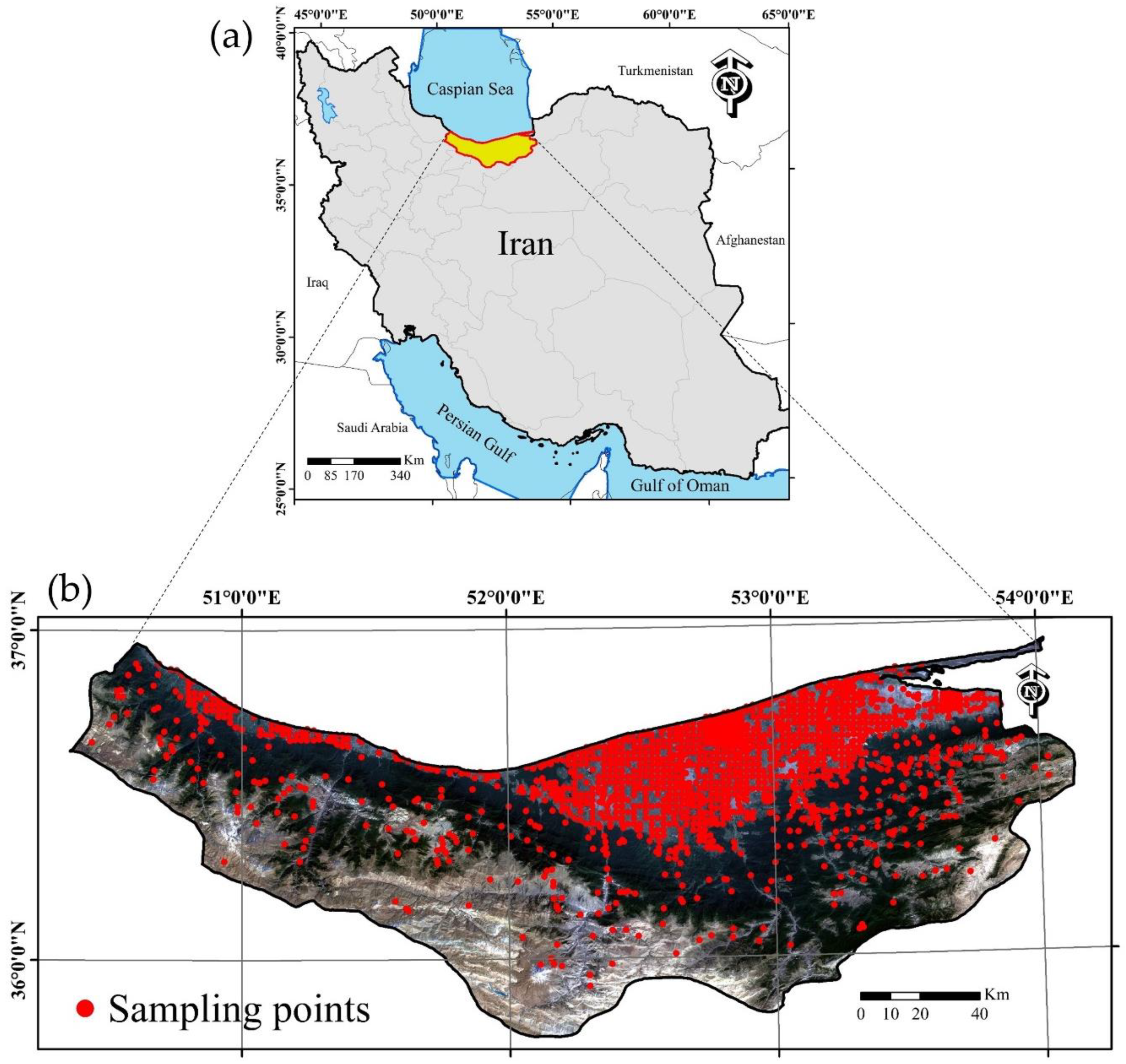
2.1. Study Area
2.2. Soil Data
2.3. Environmental Covariates
Selection of Environmental Covariates
2.4. Predictive Models
2.4.1. Backpropagation (BP) Algorithm
2.4.2. Genetic Algorithm (GA)
2.4.3. Particle Swarm Optimization (PSO)
2.4.4. Bat Algorithms (BAT)
2.4.5. Monarch Butterfly Optimization (MBO) Algorithm
2.5. Accuracy Assessment and Uncertainty Analysis
3. Results
3.1. Summary Statistics
3.2. Accuracy Assessment and Uncertainty Analysis
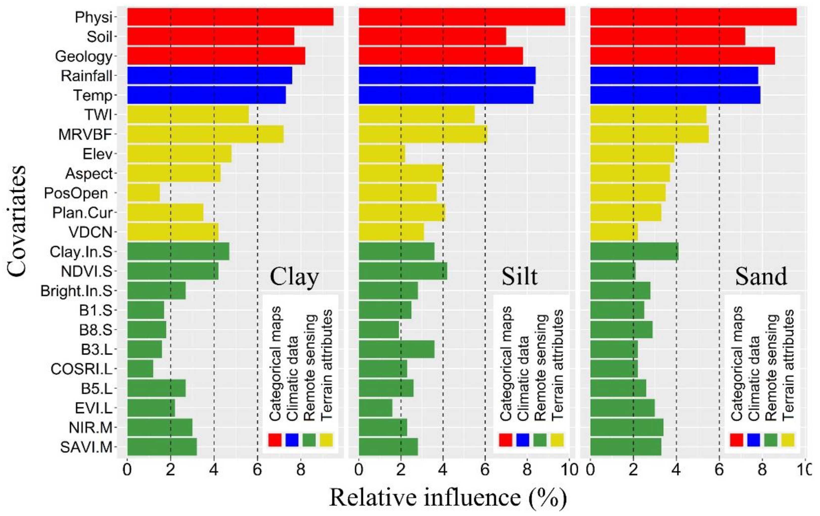
3.3. Covariate Importance
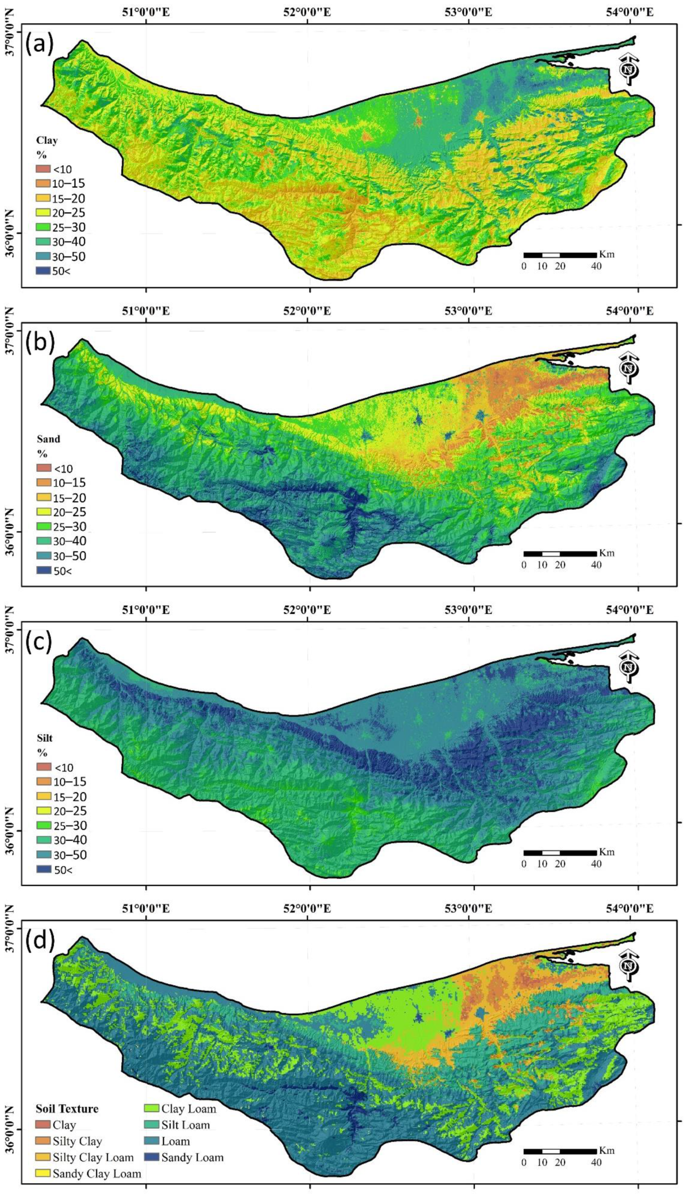
3.4. Spatial Prediction of Soil PSFs
4. Discussion
4.1. Environmental Covariates
4.2. Performance of Hybridized Models and Output Maps
5. Conclusions
Supplementary Materials
Author Contributions
Funding
Informed Consent Statement
Data Availability Statement
Acknowledgments
Conflicts of Interest
Appendix A

| No. | Covariates | Code | Definition |
|---|---|---|---|
| 1 | Geology map | Geology | Polygon map prepared by SWRI |
| 2 | Soil map | Soil | Polygon map prepared by SWRI |
| 3 | Physiography map | Physi | Polygon map prepared by SWRI |
| 4 | Annual rainfall (mm) | Rainfall | It is derived from the monthly rainfall values |
| 5 | Mean annual temperature (°C) | Temp | It is derived from the monthly temperature values |
| 6 | Aspect (°C) | Aspect | The compass direction of the maximum rate of change |
| 7 | Catchment area | Cat.Area | Area from which rainfall flows into a river |
| 8 | Catchment slope (degrees) | Cat.Slo. | Average gradient above flow path |
| 9 | Channel networks base level | CNBL | The interpolated channel network base level elevations |
| 10 | Elevation (m) | Elev | Height above sea level |
| 11 | Flow accumulation (number of cells) | Fl.Ac | Calculates accumulated flow |
| 12 | Multi-resolution Valley Bottom Flatness Index | MRVBF | Measure of flatness and lowness |
| 13 | Openness | NegOpen | How wide a landscape can be viewed from any position |
| 14 | Openness | PosOpen | How wide a landscape can be viewed from any position |
| 15 | Plan curvature (radians / m) | Plan.Cur | The curvature of a contour line |
| 16 | Relative Slope Position | Re.Slope.Posi | The position of one point relative to the ridge and valley of a slope |
| 17 | Slope Length factor | LS factor | Slope Length and Steepness factor |
| 18 | Topographic Wetness index | TWI | ln (specific catchment area/slope angle) |
| 19 | Total Insolation (kWh / m2) | To.In | Calculate the total incoming solar radiation |
| 20 | Upslope Curvature | Ups.Cur | The distance weighted average local curvature |
| 21 | Valley Depth (m) | Va.Dep | The vertical distance to a channel network base level |
| 22 | Vertical distance to channel networks (m) | VDCN | The altitude above the channel network |
| 23 | Wind Effect | WE | The Wind Effect is a dimensionless index |
| 24 | Coastal aerosol of Sentinel-2 | B1.S | Wavelength of 0.442 μm |
| 25 | Blue band of Sentinel-2 | B2.S | Wavelength of 0.492 μm |
| 26 | Green band of Sentinel-2 | B3.S | Wavelength of 0.559 μm |
| 27 | Red band of Sentinel-2 | B4.S | Wavelength of 0.664 μm |
| 28 | Vegetation Red Edge of Sentinel-2 | B5.S | Wavelength of 0.704 μm |
| 29 | Vegetation Red Edge of Sentinel-2 | B6.S | Wavelength of 0.740 μm |
| 30 | Vegetation Red Edge of Sentinel-2 | B7.S | Wavelength of 0.782 μm |
| 31 | Near-infra red of Sentinel-2 | B8.S | Wavelength of 0.832 μm |
| 32 | Shortwave IR-1 band of Sentinel-2 | B9.S | Wavelength of 0.945 μm |
| 33 | Shortwave IR-2 band of Sentinel-2 | B10.S | Wavelength of 1.373 μm |
| 34 | Normalized Difference Vegetation Index | NDVI.S | (NIR−GREEN / NIR + GREEN) |
| 35 | Enhanced Vegetation Index of Sentinel-2 | EVI.S | (2.5 × (Band4 − Band3)/(Band4 + 6× Band 3–7.7 × Band1 + 1) |
| 36 | Transformed vegetation index of Sentinel-2 | TVI.S | (Band5 − Band3/ Band5 + Band3) |
| 37 | Soil Adjusted Vegetation Index of Sentinel-2 | SAVI.S | (Band4 − Band3/ Band4 + Band3 + 0.5) × (1 + 0.5)) |
| 38 | Land Surface Water Index of Sentinel-2 | LSWI.S | (NIR − shortwave infrared)/ (NIR+shortwave infrared) |
| 39 | Brightness Index of Sentinel-2 | Bright.In.S | ((RED)2 + (NIR)2)0.5 |
| 40 | Clay Index of Sentinel-2 | Clay.In.S | (SWIR-1 / SWIR-2) |
| 41 | Normalized Difference Salinity Index of Sentinel-2 | Salin.In.S | (Red-NIR)/(Red + NIR) |
| 42 | Carbonate Index of Sentinel-2 | Carbonat.In.S | (RED / GREEN) |
| 43 | Gypsum index of Sentinel-2 | Gypsum.In.S | (SWIR-1 − NIR) / (SWIR-1 + NIR) |
| 44 | Blue band of Landsat-8 | B1.L | Wavelength of 0.450–0.515 μm of Landsat 8 spectral band |
| 45 | Green band of Landsat-8 | B2.L | Wavelength of 0.525–0.600 μm of Landsat 8 spectral band |
| 46 | Red band of Landsat-8 | B3.L | Wavelength of 0.630–0.680 μm of Landsat 8 spectral band |
| 47 | Near infrared band of Landsat-8 | B4.L | Wavelength of 0.845–0.885 μm of Landsat 8 spectral band |
| 48 | Shortwave Infrared-1 band of Landsat-8 | B5.L | Wavelength of 1.560–1.660 μm of Landsat 8 spectral band |
| 49 | Shortwave Infrared-2 band of Landsat-8 | B6.L | Wavelength of 2.100–2.300 μm of Landsat 8 spectral band |
| 50 | Normalized Difference Vegetation Index of Landsat-8 | NDVI.L | (NIR − RED) / (NIR + RED) |
| 51 | Enhanced Vegetation Index of Landsat-8 | EVI.L | (NIR − RED) / (NIR + C1 × RED−C2 × BLUE + L) |
| 52 | Soil Adjusted Vegetation Index of Landsat-8 | SAVI.L | (1 + L) × (NIR − RED) / (NIR + RED + L) |
| 53 | Normalized difference moisture index of Landsat-8 | NDMI.L | (Band4 − Band5/ Band4 + Band5) |
| 54 | Combined spectral response index of Landsat-8 | COSRI.L | [Blue + Green)/(Red + NIR)] × NDVI.L |
| 55 | Brightness Index of Landsat-8 | Bright.In.L | ((RED)2 + (NIR)2)0.5 |
| 56 | Clay Index of Landsat-8 | Clay.In.L | (SWIR-1/SWIR-2) |
| 57 | Salinity Index of Landsat-8 | Salinity.In.L | Band 3/Band 4 |
| 58 | Carbonate Index of Landsat-8 | Carbon.In.L | (RED / GREEN) |
| 59 | Gypsum index of Landsat-8 | Gypsum.In.L | (SWIR-1 − NIR) / (SWIR-1 + NIR) |
| 60 | MODIS Night Temperature | Temp.M | Land Surface Temperature/Emissivity Daily L3 Global 1km |
| 61 | MODIS Near Infrared | NIR.M | Wavelength of 0.841–0.876 μm of MODIS spectral band |
| 62 | Normalized Difference Vegetation Index of MODIS | NDVI.M | (NIR – GREEN / NIR+ GREEN) |
| 63 | Soil Adjusted Vegetation Index of MODIS | SAVI.M | (1 + L) × ( NIR − RED) / (NIR + RED + L) |
| 64 | Brightness Index of MODIS | Brigh.Index.M | ((MODIS RED)2 + (MODIS NIR)2)0.5 |
References
- Kome, G.K.; Enang, R.K.; Tabi, F.O.; Yerima, B.P.K. Influence of Clay Minerals on Some Soil Fertility Attributes: A Review. Open J. Soil Sci. 2019, 9, 155–188. [Google Scholar] [CrossRef] [Green Version]
- Morgan, R.; Quinton, J.; Smith, R.; Govers, G.; Poesen, J.; Auerswald, K.; Chisci, G.; Torri, D.; Styczen, M. The European Soil Erosion Model (EUROSEM): A dynamic approach for predicting sediment transport from fields and small catchments. Earth Surf. Process. Landf. J. Br. Geomorphol. Group 1998, 23, 527–544. [Google Scholar] [CrossRef]
- Poggio, L.; Gimona, A. 3D mapping of soil texture in Scotland. Geoderma Reg. 2017, 9, 5–16. [Google Scholar] [CrossRef]
- Wang, W.J.; Dalal, R.C.; Moody, P.W.; Smith, C.J. Relationships of soil respiration to microbial biomass, substrate availability and clay content. Soil Biol. Biochem. 2003, 35, 273–284. [Google Scholar] [CrossRef]
- Koseva, I.S.; Watmough, S.A.; Aherne, J. Estimating base cation weathering rates in Canadian forest soils using a simple texture-based model. Biogeochemistry 2010, 101, 183–196. [Google Scholar] [CrossRef]
- Ghiri, M.N.; Abtahi, A. Factors affecting potassium fixation in calcareous soils of southern Iran. Arch. Agron. Soil Sci. 2012, 58, 335–352. [Google Scholar] [CrossRef]
- Goli-Kalanpa, E.; Roozitalab, M.; Malakouti, M. Potassium availability as related to clay mineralogy and rates of potassium application. Commun. Soil Sci. Plant Anal. 2008, 39, 2721–2733. [Google Scholar] [CrossRef]
- Vaughan, E.; Matos, M.; Ríos, S.; Santiago, C.; Marín-Spiotta, E. Clay and climate are poor predictors of regional-scale soil carbon storage in the US Caribbean. Geoderma 2019, 354, 113841. [Google Scholar] [CrossRef]
- Xu, H.; Liu, K.; Zhang, W.; Rui, Y.; Zhang, J.; Wu, L.; Colinet, G.; Huang, Q.; Chen, X.; Xu, M. Long-term fertilization and intensive cropping enhance carbon and nitrogen accumulated in soil clay-sized particles of red soil in South China. J. Soils Sediments 2020, 20, 1824–1833. [Google Scholar] [CrossRef]
- Bockheim, J.; Hartemink, A. Distribution and classification of soils with clay-enriched horizons in the USA. Geoderma 2013, 209, 153–160. [Google Scholar] [CrossRef]
- Amirian-Chakan, A.; Minasny, B.; Taghizadeh-Mehrjardi, R.; Akbarifazli, R.; Darvishpasand, Z.; Khordehbin, S. Some practical aspects of predicting texture data in digital soil mapping. Soil Tillage Res. 2019, 194, 104289. [Google Scholar] [CrossRef]
- Wadoux, A.M.C. Using deep learning for multivariate mapping of soil with quantified un-certainty. Geoderma 2019, 351, 59–70. [Google Scholar] [CrossRef] [Green Version]
- Wang, Z.; Shi, W. Mapping soil particle-size fractions: A comparison of compositional kriging and log-ratio kriging. J. Hydrol. 2017, 546, 526–541. [Google Scholar] [CrossRef]
- Walvoort, D.J.; de Gruijter, J.J. Compositional kriging: A spatial interpolation method for compositional data. Math. Geol. 2001, 33, 951–966. [Google Scholar] [CrossRef]
- Pahlavan-Rad, M.R.; Akbarimoghaddam, A. Spatial variability of soil texture fractions and pH in a flood plain (case study from eastern Iran). Catena 2018, 160, 275–281. [Google Scholar] [CrossRef]
- Taghizadeh-Mehrjardi, R.; Toomanian, N.; Khavaninzadeh, A.; Jafari, A.; Triantafilis, J. Predicting and mapping of soil particle-size fractions with adaptive neuro-fuzzy inference and ant colony optimization in central I ran. Eur. J. Soil Sci. 2016, 67, 707–725. [Google Scholar] [CrossRef]
- Zhao, Z.; Chow, T.L.; Rees, H.W.; Yang, Q.; Xing, Z.; Meng, F.-R. Predict soil texture distributions using an artificial neural network model. Comput. Electron. Agric. 2009, 65, 36–48. [Google Scholar] [CrossRef]
- Song, X.-D.; Liu, F.; Zhang, G.-L.; Li, D.-C.; Zhao, Y.-G. Estimation of Soil Texture at a Regional Scale Using Local Soil-Landscape Models. Soil Sci. 2016, 181, 435–445. [Google Scholar] [CrossRef]
- Wu, W.; Li, A.-D.; He, X.-H.; Ma, R.; Liu, H.-B.; Lv, J.-K. A comparison of support vector machines, artificial neural network and classification tree for identifying soil texture classes in southwest China. Comput. Electron. Agric. 2018, 144, 86–93. [Google Scholar] [CrossRef]
- Ding, X.; Zhao, Z.; Yang, Q.; Chen, L.; Tian, Q.; Li, X.; Meng, F.-R. Model prediction of depth-specific soil texture distributions with artificial neural network: A case study in Yunfu, a typical area of Udults Zone, South China. Comput. Electron. Agric. 2020, 169, 105217. [Google Scholar] [CrossRef]
- Khanbabakhani, E.; Torkashvand, A.M.; Mahmoodi, M.A. The possibility of preparing soil texture class map by artificial neural networks, inverse distance weighting, and geostatistical methods in Gavoshan dam basin, Kurdistan Province, Iran. Arab. J. Geosci. 2020, 13, 1–14. [Google Scholar] [CrossRef]
- Wang, Z.; Shi, W.; Zhou, W.; Li, X.; Yue, T. Comparison of additive and isometric log-ratio transformations combined with machine learning and regression kriging models for mapping soil particle size fractions. Geoderma 2020, 365, 114214. [Google Scholar] [CrossRef]
- Greve, M.H.; Kheir, R.B.; Greve, M.B.; Bøcher, P.K. Quantifying the ability of environmental parameters to predict soil texture fractions using regression-tree model with GIS and LIDAR data: The case study of Denmark. Ecol. Indic. 2012, 18, 1–10. [Google Scholar] [CrossRef]
- Akpa, S.I.; Odeh, I.O.; Bishop, T.F.; Hartemink, A.E. Digital mapping of soil particle-size fractions for Nigeria. Soil Sci. Soc. Am. J. 2014, 78, 1953–1966. [Google Scholar] [CrossRef] [Green Version]
- Mehrabi-Gohari, E.; Matinfar, H.R.; Jafari, A.; Taghizadeh-Mehrjardi, R.; Triantafilis, J. The Spatial Prediction of Soil Texture Fractions in Arid Regions of Iran. Soil Syst. 2019, 3, 65. [Google Scholar] [CrossRef] [Green Version]
- Heung, B.; Ho, H.C.; Zhang, J.; Knudby, A.; Bulmer, C.E.; Schmidt, M.G. An overview and comparison of machine-learning techniques for classification purposes in digital soil mapping. Geoderma 2016, 265, 62–77. [Google Scholar] [CrossRef]
- Vaheddoost, B.; Guan, Y.; Mohammadi, B. Application of hybrid ANN-whale optimization model in evaluation of the field capacity and the permanent wilting point of the soils. Environ. Sci. Pollut. Res. 2020, 27, 13131–13141. [Google Scholar] [CrossRef] [PubMed]
- Nabipour, N.; Dehghani, M.; Mosavi, A.; Shamshirband, S. Short-Term Hydrological Drought Forecasting Based on Different Nature-Inspired Optimization Algorithms Hybridized With Artificial Neural Networks. IEEE Access 2020, 8, 15210–15222. [Google Scholar] [CrossRef]
- Taghavifar, H.; Khalilarya, S.; Jafarmadar, S. Diesel engine spray characteristics prediction with hybridized artificial neural network optimized by genetic algorithm. Energy 2014, 71, 656–664. [Google Scholar] [CrossRef]
- Termeh, S.V.R.; Kornejady, A.; Pourghasemi, H.R.; Keesstra, S. Flood susceptibility mapping using novel ensembles of adaptive neuro fuzzy inference system and metaheuristic algorithms. Sci. Total Environ. 2018, 615, 438–451. [Google Scholar] [CrossRef]
- Liu, Y.; Xie, S.; Zheng, L.; Li, T.; Sun, Y.; Ma, L.; Lin, Z.; Grathwohl, P.; Lohmann, R. Air-soil diffusive exchange of PAHs in an urban park of Shanghai based on polyethylene passive sampling: Vertical distribution, vegetation influence and diffusive flux. Sci. Total Environ. 2019, 689, 734–742. [Google Scholar] [CrossRef] [Green Version]
- Moayedi, H.; Gör, M.; Khari, M.; Foong, L.K.; Bahiraei, M.; Bui, D.T. Hybridizing four wise neural-metaheuristic paradigms in predicting soil shear strength. Measurement 2020, 156, 107576. [Google Scholar] [CrossRef]
- Dehghani, M.; Montazeri, Z.; Dehghani, A.; Malik, O.P.; Morales-Menendez, R.; Dhiman, G.; Nouri, N.; Ehsanifar, A.; Guerrero, J.M.; Ramirez-Mendoza, R.A. Binary Spring Search Algorithm for Solving Various Optimization Problems. Appl. Sci. 2021, 11, 1286. [Google Scholar] [CrossRef]
- Mohammadi, B.; Guan, Y.; Aghelpour, P.; Emamgholizadeh, S.; Pillco Zolá, R.; Zhang, D. Simulation of Titicaca Lake Water Level Fluctuations Using Hybrid Machine Learning Technique Integrated with Grey Wolf Optimizer Algorithm. Water 2020, 12, 3015. [Google Scholar] [CrossRef]
- Zhou, N.; Lau, L.; Bai, R.; Moore, T. A Genetic Optimization Resampling Based Particle Filtering Algorithm for Indoor Target Tracking. Remote Sens. 2021, 13, 132. [Google Scholar] [CrossRef]
- De Martonne, E. Une nouvelle function climatologique: L’indice d’aridité. Meteorologie 1926, 2, 449–459. [Google Scholar]
- Emadi, M.; Shahriari, A.R.; Sadegh-Zadeh, F.; Jalili Seh-Bardan, B.; Dindarlou, A. Geostatistics-based spatial distribution of soil moisture and temperature regime classes in Mazandaran province, northern Iran. Arch. Agron. Soil Sci. 2016, 62, 502–522. [Google Scholar] [CrossRef]
- Emadi, M.; Baghernejad, M.; Bahmanyar, M.A.; Morovvat, A. Changes in soil inorganic phosphorous pools along a precipitation gradient in northern Iran. Int. J. For. Soil Eros. (IJFSE) 2012, 2, 143–147. [Google Scholar]
- Khormali, F.; Ghergherechi, S.; Kehl, M.; Ayoubi, S. Soil formation in loess-derived soils along a subhumid to humid climate gradient, Northeastern Iran. Geoderma 2012, 179, 113–122. [Google Scholar] [CrossRef]
- Gee, G.W.; Bauder, J.W. Particle-size analysis. Methods Soil Anal. 1986, 5, 383–411. [Google Scholar]
- Gerakis, A.; Baer, B. A computer program for soil textural classification. Soil Sci. Soc. Am. J. 1999, 63, 807–808. [Google Scholar] [CrossRef]
- McBratney, A.B.; Mendonça Santos, M.L.; Minasny, B. On digital soil mapping. Geoderma 2003, 117, 3–52. [Google Scholar] [CrossRef]
- Gallant, J.C.; Dowling, T.I. A multiresolution index of valley bottom flatness for mapping depositional areas. Water Resour. Res. 2003, 39, 1347. [Google Scholar] [CrossRef]
- Wang, Z.; Shi, W. Robust variogram estimation combined with isometric log-ratio transformation for improved accuracy of soil particle-size fraction mapping. Geoderma 2018, 324, 56–66. [Google Scholar] [CrossRef]
- Mutanga, O.; Skidmore, A.K. Narrow band vegetation indices overcome the saturation problem in biomass estimation. Int. J. Remote Sens. 2004, 25, 3999–4014. [Google Scholar] [CrossRef]
- Escadafal, R. Soil spectral properties and their relationships with environmental parameters-examples from arid regions. In Imaging Spectrometry—A Tool for Environmental Observations; Springer: Dordrecht, The Netherlands, 1994; pp. 71–87. [Google Scholar]
- Serrano, J.; Shahidian, S.; Marques da Silva, J. Evaluation of normalized difference water index as a tool for monitoring pasture seasonal and inter-annual variability in a Mediterranean agro-silvo-pastoral system. Water 2019, 11, 62. [Google Scholar] [CrossRef] [Green Version]
- Xiao, X.; Hollinger, D.; Aber, J.; Goltz, M.; Davidson, E.A.; Zhang, Q.; Moore III, B. Satellite-based modeling of gross primary production in an evergreen needleleaf forest. Remote Sens. Environ. 2004, 89, 519–534. [Google Scholar] [CrossRef]
- Dogan, O.K.; Akyurek, Z.; Beklioglu, M. Identification and mapping of submerged plants in a shallow lake using quickbird satellite data. J. Environ. Manag. 2009, 90, 2138–2143. [Google Scholar] [CrossRef]
- Khan, N.M.; Rastoskuev, V.V.; Sato, Y.; Shiozawa, S. Assessment of hydrosaline land degradation by using a simple approach of remote sensing indicators. Agric. Water Manag. 2005, 77, 96–109. [Google Scholar] [CrossRef]
- Nield, S.; Boettinger, J.; Ramsey, R. Digitally mapping gypsic and natric soil areas using Landsat ETM data. Soil Sci. Soc. Am. J. 2007, 71, 245–252. [Google Scholar] [CrossRef] [Green Version]
- Boettinger, J.; Ramsey, R.; Bodily, J.; Cole, N.; Kienast-Brown, S.; Nield, S.; Saunders, A.; Stum, A. Landsat spectral data for digital soil mapping. In Digital Soil Mapping with Limited Data; Springer: Dordrecht, The Netherlands, 2008; pp. 193–202. [Google Scholar]
- Fick, S.E.; Hijmans, R.J. WorldClim 2: New 1-km spatial resolution climate surfaces for global land areas. Int. J. Climatol. 2017, 37, 4302–4315. [Google Scholar] [CrossRef]
- Karegowda, A.G.; Manjunath, A.; Jayaram, M. Comparative study of attribute selection using gain ratio and correlation based feature selection. Int. J. Inf. Technol. Knowl. Manag. 2010, 2, 271–277. [Google Scholar]
- Hall, D.B. Zero-inflated Poisson and binomial regression with random effects: A case study. Biometrics 2000, 56, 1030–1039. [Google Scholar] [CrossRef]
- Haykin, S. Neural Networks: A Comprehensive Foundation; Prentice Hall PTR: Upper Saddle River, NJ, USA, 1998. [Google Scholar]
- Lazzús, J.; Vega-Jorquera, P.; Palma-Chilla, L.; Stepanova, M.; Romanova, N. D st Index Forecast Based on Ground-Level Data Aided by Bio-Inspired Algorithms. Space Weather 2019, 17, 1487–1506. [Google Scholar] [CrossRef] [Green Version]
- Zhang, W.; Goh, A.T. Multivariate adaptive regression splines and neural network models for prediction of pile drivability. Geosci. Front. 2016, 7, 45–52. [Google Scholar] [CrossRef] [Green Version]
- Abeyrathna, K.D.; Jeenanunta, C. Training Artificial Neural Networks With Improved Particle Swarm Optimization: Case of Electricity Demand Forecasting in Thailand. In Handbook of Research on Advancements of Swarm Intelligence Algorithms for Solving Real-World Problems; IGI Global: Hershey, PA, USA, 2020; pp. 63–77. [Google Scholar]
- Sarangi, P.K.; Singh, N.; Swain, D.; Chauhan, R.; Singh, R. Short term load forecasting using neuro genetic hybrid approach: Results analysis with different network architectures. J. Theor. Appl. Inf. Technol. 2009, 5, 109–116. [Google Scholar]
- Eberhart, R.; Kennedy, J. A new optimizer using particle swarm theory. In Proceedings of the MHS’95, Sixth International Symposium on Micro Machine and Human Science, Nagoya, Japan, 4–6 October 1995; pp. 39–43. [Google Scholar]
- Shariati, M.; Mafipour, M.S.; Mehrabi, P.; Bahadori, A.; Zandi, Y.; Salih, M.N.; Nguyen, H.; Dou, J.; Song, X.; Poi-Ngian, S. Application of a hybrid artificial neural network-particle swarm optimization (ANN-PSO) model in behavior prediction of channel shear connectors embedded in normal and high-strength concrete. Appl. Sci. 2019, 9, 5534. [Google Scholar] [CrossRef] [Green Version]
- Yang, X.-S. A new metaheuristic bat-inspired algorithm. In Nature Inspired Cooperative Strategies for Optimization (NICSO 2010); Springer: Berlin/Heidelberg, Germany, 2010; pp. 65–74. [Google Scholar]
- Dong, J.; Wu, L.; Liu, X.; Li, Z.; Gao, Y.; Zhang, Y.; Yang, Q. Estimation of daily dew point temperature by using bat algorithm optimization based extreme learning machine. Appl. Therm. Eng. 2020, 165, 114569. [Google Scholar] [CrossRef]
- Devikanniga, D.; Raj, R.J.S. Classification of osteoporosis by artificial neural network based on monarch butterfly optimisation algorithm. Healthc. Technol. Lett. 2018, 5, 70–75. [Google Scholar] [CrossRef] [PubMed]
- Wang, G.-G.; Deb, S.; Cui, Z. Monarch butterfly optimization. Neural Comput. Appl. 2019, 31, 1995–2014. [Google Scholar] [CrossRef] [Green Version]
- Hitziger, M.; Ließ, M. Comparison of three supervised learning methods for digital soil mapping: Application to a complex terrain in the Ecuadorian Andes. Appl. Environ. Soil Sci. 2014, 2014, 809495. [Google Scholar] [CrossRef]
- Wilding, L. Spatial variability: Its documentation, accomodation and implication to soil surveys. In Proceedings of the Soil Spatial Variability, Las Vegas NV, USA, 30 November–1 December 1984; pp. 166–194. [Google Scholar]
- Kiani-Harchegani, M.; Sadeghi, S.H.; Asadi, H. Comparing grain size distribution of sediment and original soil under raindrop detachment and raindrop-induced and flow transport mechanism. Hydrol. Sci. J. 2018, 63, 312–323. [Google Scholar] [CrossRef]
- Lazzús, J.; Vega, P.; Rojas, P.; Salfate, I. Forecasting the Dst index using a swarm-optimized neural network. Space Weather 2017, 15, 1068–1089. [Google Scholar] [CrossRef]
- Khormali, F.; Kehl, M. Micromorphology and development of loess-derived surface and buried soils along a precipitation gradient in Northern Iran. Quat. Int. 2011, 234, 109–123. [Google Scholar] [CrossRef]
- Akpa, S.I.; Odeh, I.O.; Bishop, T.F.; Hartemink, A.E.; Amapu, I.Y. Total soil organic carbon and carbon sequestration potential in Nigeria. Geoderma 2016, 271, 202–215. [Google Scholar] [CrossRef]
- Law-Ogbomo, K.; Nwachokor, M. Variability in selected soil physic-chemical properties of five soils formed on different parent materials in southeastern Nigeria. Res. J. Agric. Biol. Sci 2010, 6, 14–19. [Google Scholar]
- Wang, D.-C.; Zhang, G.-L.; Zhao, M.-S.; Pan, X.-Z.; Zhao, Y.-G.; Li, D.-C.; Macmillan, B. Retrieval and mapping of soil texture based on land surface diurnal temperature range data from MODIS. PLoS ONE 2015, 10, e0125814. [Google Scholar] [CrossRef] [PubMed]
- Gomez, C.; Dharumarajan, S.; Féret, J.-B.; Lagacherie, P.; Ruiz, L.; Sekhar, M. Use of sentinel-2 time-series images for classification and uncertainty analysis of inherent biophysical property: Case of soil texture mapping. Remote Sens. 2019, 11, 565. [Google Scholar] [CrossRef] [Green Version]
- Luo, H.; Zheng, Y. The camparison of citrus canopy spectral characteristics obtained by the HJ-1A/HSI and ASD field spectrometer. In Proceedings of the 2012 9th International Conference on Fuzzy Systems and Knowledge Discovery, Chongqing, China, 29–31 May 2012; pp. 1977–1980. [Google Scholar]
- Bousbih, S.; Zribi, M.; Pelletier, C.; Gorrab, A.; Lili-Chabaane, Z.; Baghdadi, N.; Ben Aissa, N.; Mougenot, B. Soil texture estimation using radar and optical data from Sentinel-1 and Sentinel-2. Remote Sens. 2019, 11, 1520. [Google Scholar] [CrossRef] [Green Version]
- Lagacherie, P. Digital soil mapping: A state of the art. In Digital Soil Mapping with Limited Data; Springer: Dordrecht, The Netherlands, 2008; pp. 3–14. [Google Scholar]
- Shahriari, M.; Delbari, M.; Afrasiab, P.; Pahlavan-Rad, M.R. Predicting regional spatial distribution of soil texture in floodplains using remote sensing data: A case of southeastern Iran. Catena 2019, 182, 104149. [Google Scholar] [CrossRef]
- De Carvalho Junior, W.; Lagacherie, P.; da Silva Chagas, C.; Calderano Filho, B.; Bhering, S.B. A regional-scale assessment of digital mapping of soil attributes in a tropical hillslope environment. Geoderma 2014, 232, 479–486. [Google Scholar] [CrossRef] [Green Version]
- Liao, K.; Xu, S.; Wu, J.; Zhu, Q. Spatial estimation of surface soil texture using remote sensing data. Soil Sci. Plant Nutr. 2013, 59, 488–500. [Google Scholar] [CrossRef]
- Gholizadeh, A.; Žižala, D.; Saberioon, M.; Borůvka, L. Soil organic carbon and texture retrieving and mapping using proximal, airborne and Sentinel-2 spectral imaging. Remote Sens. Environ. 2018, 218, 89–103. [Google Scholar] [CrossRef]
- Da Silva Chagas, C.; de Carvalho Junior, W.; Bhering, S.B.; Calderano Filho, B. Spatial prediction of soil surface texture in a semiarid region using random forest and multiple linear regressions. Catena 2016, 139, 232–240. [Google Scholar] [CrossRef]
- Bishop, T.; McBratney, A. A comparison of prediction methods for the creation of field-extent soil property maps. Geoderma 2001, 103, 149–160. [Google Scholar] [CrossRef]
- Adhikari, K.; Kheir, R.B.; Greve, M.B.; Bøcher, P.K.; Malone, B.P.; Minasny, B.; McBratney, A.B.; Greve, M.H. High-resolution 3-D mapping of soil texture in Denmark. Soil Sci. Soc. Am. J. 2013, 77, 860–876. [Google Scholar] [CrossRef]
- Muzzamal, M.; Huang, J.; Nielson, R.; Sefton, M.; Triantafilis, J. Mapping soil particle-size fractions using additive log-ratio (ALR) and isometric log-ratio (ILR) transformations and proximally sensed ancillary data. Clays Clay Miner. 2018, 66, 9–27. [Google Scholar] [CrossRef]
- Gasmi, A.; Gomez, C.; Lagacherie, P.; Zouari, H. Surface soil clay content mapping at large scales using multispectral (VNIR–SWIR) ASTER data. Int. J. Remote Sens. 2019, 40, 1506–1533. [Google Scholar] [CrossRef]
- Mulder, V.L.; Lacoste, M.; Richer-de-Forges, A.; Arrouays, D. GlobalSoilMap France: High-resolution spatial modelling the soils of France up to two meter depth. Sci. Total Environ. 2016, 573, 1352–1369. [Google Scholar] [CrossRef] [PubMed]
- Hengl, T.; Heuvelink, G.B.; Kempen, B.; Leenaars, J.G.; Walsh, M.G.; Shepherd, K.D.; Sila, A.; MacMillan, R.A.; de Jesus, J.M.; Tamene, L. Mapping soil properties of Africa at 250 m resolution: Random forests significantly improve current predictions. PLoS ONE 2015, 10, e0125814. [Google Scholar] [CrossRef]
- Kouchami-Sardoo, I.; Shirani, H.; Esfandiarpour-Boroujeni, I.; Besalatpour, A.; Hajabbasi, M. Prediction of soil wind erodibility using a hybrid Genetic algorithm–Artificial neural network method. Catena 2020, 187, 104315. [Google Scholar] [CrossRef]
- Mohamad, E.T.; Faradonbeh, R.S.; Armaghani, D.J.; Monjezi, M.; Majid, M.Z.A. An optimized ANN model based on genetic algorithm for predicting ripping production. Neural Comput. Appl. 2017, 28, 393–406. [Google Scholar] [CrossRef]
- Abeyrathna, K.D.; Jeenanunta, C. Hybrid particle swarm optimization with genetic algorithm to train artificial neural networks for short-term load forecasting. Int. J. Swarm Intell. Res. (IJSIR) 2019, 10, 1–14. [Google Scholar] [CrossRef] [Green Version]


| Bio-Inspired Algorithms | Hyper-Parameters | Defined Parameters |
|---|---|---|
| GA | Population size | 50 |
| Crossover rate | 0.75 | |
| Cost function | RMSE | |
| Learning algorithm | Levenberg-Marquardt | |
| Activation function | Tangent-sigmoid | |
| Selection method | Roulette Wheel | |
| Generation number | 100 | |
| Chromosome size | 9 | |
| Mutation rate | 0.06 | |
| PSO | Acceleration constants | 2.1 |
| Inertia weights | 0.9–0.6 | |
| BAT | Loudness | 0.5 |
| Pulse rate | 0.5 | |
| Frequency minimum | 0 | |
| Frequency maximum | 1 | |
| MBO | Population size | 50 |
| Maximum number of generations | 100 | |
| Max walk step (Smax) | 1.0 | |
| BAR | 5/12 | |
| Migration period (peri) | 1.2 | |
| Migration ratio (p) | 5/12 | |
| Activation function | Hyperbolic tangent |
| Min | Max | Mean | Median | SD | CV | Skewness | Kurtosis | |
|---|---|---|---|---|---|---|---|---|
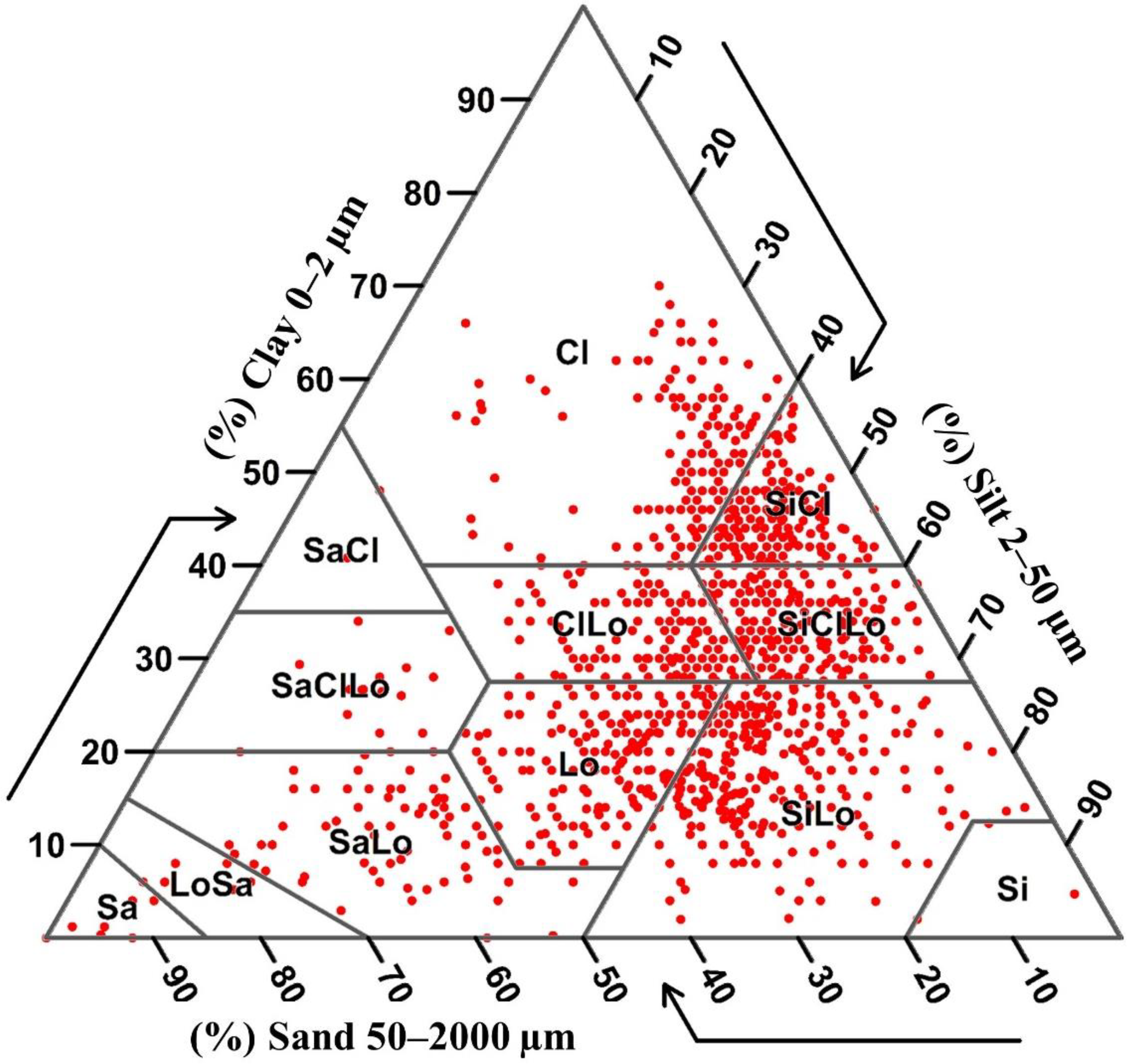
| Clay (%) | 0.2 | 70.0 | 31.4 | 31.3 | 12.51 | 39.84 | 0.13 | −0.57 |
| Silt (%) | 6.0 | 84.0 | 45.2 | 46.0 | 11.21 | 24.80 | −0.27 | 1.04 |
| Sand (%) | 1.0 | 86.0 | 23.4 | 20.0 | 14.68 | 62.73 | 1.21 | 1.50 |
| ANN Models | Clay | Silt | Sand | |||||||||
|---|---|---|---|---|---|---|---|---|---|---|---|---|
| MAE | RMSE | R2 | CCC | MAE | RMSE | R2 | CCC | MAE | RMSE | R2 | CCC | |
| BP-ANN | 6.54 | 8.10 | 0.50 | 0.51 | 5.76 | 7.34 | 0.32 | 0.25 | 6.50 | 8.70 | 0.45 | 0.49 |
| GA-ANN | 5.76 | 6.71 | 0.65 | 0.68 | 4.87 | 6.68 | 0.60 | 0.63 | 5.79 | 6.58 | 0.69 | 0.70 |
| PSO-ANN | 5.78 | 6.77 | 0.57 | 0.62 | 5.01 | 6.70 | 0.58 | 0.60 | 5.88 | 6.85 | 0.59 | 0.63 |
| BAT-ANN | 5.80 | 6.60 | 0.63 | 0.66 | 5.14 | 6.78 | 0.49 | 0.51 | 5.88 | 6.77 | 0.61 | 0.63 |
| MBO-ANN | 5.60 | 6.46 | 0.68 | 0.69 | 4.81 | 6.60 | 0.62 | 0.65 | 5.74 | 6.59 | 0.70 | 0.71 |
| ANN Models | Clay | Silt | Sand | ||||||
|---|---|---|---|---|---|---|---|---|---|
| Inside CI | Outside CI | Inside CI | Outside CI | Inside CI | Outside CI | ||||
| 5 to 95% | <5% | >95% | 5 to 95% | <5% | >95% | 6.50 | <5% | >95% | |
| BP-ANN | 78 | 12.4 | 9.6 | 72 | 14.8 | 13.2 | 81 | 10.5 | 8.5 |
| GA-ANN | 81 | 8.7 | 10.3 | 78 | 9.8 | 12.2 | 84 | 6.4 | 9.6 |
| PSO-ANN | 81 | 9.0 | 10.0 | 75 | 13.0 | 12.0 | 83 | 8.5 | 8.5 |
| BAT-ANN | 82 | 7.2 | 10.8 | 74 | 11.4 | 14.6 | 86 | 8.4 | 5.6 |
| MBO-ANN | 85 | 8.0 | 7.0 | 83 | 7.9 | 9.1 | 88 | 6.4 | 5.6 |
| Covariates | Clay | Silt | Sand | ||||||||||
|---|---|---|---|---|---|---|---|---|---|---|---|---|---|
| W | Sl | M | St | W | Sl | M | St | W | Sl | M | St | ||
| RS-based covariates | Sentinel-2 | 2 | 1 | 2 | - | 1 | 3 | 1 | - | - | 4 | 1 | - |
| Landsat-8 | 2 | 2 | - | - | 1 | 3 | - | - | - | 4 | - | - | |
| MODIS | - | 2 | - | - | - | 2 | - | - | - | 2 | - | - | |
| Terrain-based covariates | 1 | 1 | 4 | 1 | - | 3 | 3 | 1 | - | 5 | 2 | - | |
| Climatic data | - | - | - | 2 | - | - | - | 2 | - | - | - | 2 | |
| Categorical data | - | - | - | 3 | - | - | - | 3 | - | - | - | 3 | |
Publisher’s Note: MDPI stays neutral with regard to jurisdictional claims in published maps and institutional affiliations. |
© 2021 by the authors. Licensee MDPI, Basel, Switzerland. This article is an open access article distributed under the terms and conditions of the Creative Commons Attribution (CC BY) license (http://creativecommons.org/licenses/by/4.0/).
Share and Cite
Taghizadeh-Mehrjardi, R.; Emadi, M.; Cherati, A.; Heung, B.; Mosavi, A.; Scholten, T. Bio-Inspired Hybridization of Artificial Neural Networks: An Application for Mapping the Spatial Distribution of Soil Texture Fractions. Remote Sens. 2021, 13, 1025. https://0-doi-org.brum.beds.ac.uk/10.3390/rs13051025
Taghizadeh-Mehrjardi R, Emadi M, Cherati A, Heung B, Mosavi A, Scholten T. Bio-Inspired Hybridization of Artificial Neural Networks: An Application for Mapping the Spatial Distribution of Soil Texture Fractions. Remote Sensing. 2021; 13(5):1025. https://0-doi-org.brum.beds.ac.uk/10.3390/rs13051025
Chicago/Turabian StyleTaghizadeh-Mehrjardi, Ruhollah, Mostafa Emadi, Ali Cherati, Brandon Heung, Amir Mosavi, and Thomas Scholten. 2021. "Bio-Inspired Hybridization of Artificial Neural Networks: An Application for Mapping the Spatial Distribution of Soil Texture Fractions" Remote Sensing 13, no. 5: 1025. https://0-doi-org.brum.beds.ac.uk/10.3390/rs13051025