Article

Sea Level Fusion of Satellite Altimetry and Tide Gauge Data by Deep Learning in the Mediterranean Sea

1
School of Geodesy and Geomatics, Wuhan University, Wuhan 430079, China
2
MOE Key Laboratory of Geospace Environment and Geodesy, Wuhan University, Wuhan 430079, China
3
Chinese Academic of Surveying and Mapping, Beijing 100830, China
4
Helmholtz Centre Potsdam–GFZ German Research Centre for Geosciences, 14473 Potsdam, Germany
*
Author to whom correspondence should be addressed.
Submission received: 15 January 2021 / Revised: 16 February 2021 / Accepted: 25 February 2021 / Published: 28 February 2021
(This article belongs to the Special Issue Satellite Altimetry: Technology and Application in Geodesy)

Abstract

:
Satellite altimetry and tide gauges are the two main techniques used to measure sea level. Due to the limitations of satellite altimetry, a high-quality unified sea level model from coast to open ocean has traditionally been difficult to achieve. This study proposes a fusion approach of altimetry and tide gauge data based on a deep belief network (DBN) method. Taking the Mediterranean Sea as the case study area, a progressive three-step experiment was designed to compare the fused sea level anomalies from the DBN method with those from the inverse distance weighted (IDW) method, the kriging (KRG) method and the curvature continuous splines in tension (CCS) method for different cases. The results show that the fusion precision varies with the methods and the input measurements. The precision of the DBN method is better than that of the other three methods in most schemes and is reduced by approximately 20% when the limited altimetry along-track data and in-situ tide gauge data are used. In addition, the distribution of satellite altimetry data and tide gauge data has a large effect on the other three methods but less impact on the DBN model. Furthermore, the sea level anomalies in the Mediterranean Sea with a spatial resolution of 0.25° × 0.25° generated by the DBN model contain more spatial distribution information than others, which means the DBN can be applied as a more feasible and robust way to fuse these two kinds of sea levels.

Graphical Abstract

1. Introduction

Sea level rise, which is mainly caused by increasing ocean heat content and melting ice [1], has already become one of the most harmful climate change consequences. Its impacts include life-threatening natural disasters and adverse effects on harbor management, agriculture and even the whole ecosystem. Recent research shows that without coastal protection or adaptation and with a mean Representative Concentration Pathway 8.5 (RCP8.5) scenario, an additional 48% of the world’s land area, 52% of the global population and 46% of global assets will be at risk of flooding by 2100 as a result of the global sea level rise [2]. Thus, monitoring and even predicting sea level change is becoming more and more necessary and important, especially in coastal areas.
Tide gauges and satellite altimetry are two main technologies used to measure the sea level variation. However, each technique has its own advantages and limitations. The difficulties in building a reliable trend of sea level rise are mainly due to the sampling shortcomings of these two datasets [3]. On the one hand, the limitations of satellite altimetry have led to a lack of high-accuracy absolute sea level measurements in the near-shore areas. On the other hand, the relative sea level anomalies determined by tide gauges, the reference frame of which is different from satellite altimetry, can only represent the land boundary areas as a result of coarse spatial resolution. Thus, the sea level information in the global near-shore regions is limited, or at least, the accuracy and resolution (spatial and temporal) need to be further improved.
There are two feasible ways to solve this problem. One is to update measurement modes with new technologies; another is further mining of existing data, i.e., the fusion of multiple ocean observations. Both tide gauges and satellite altimetry have accumulated a large number of observations, but the sea level anomaly (SLA) from tide gauges should be corrected for the vertical land motion (VLM) to be consistent with that from satellite altimetry. Based on TOPEX/Poseidon and 114 globally-distributed tide gauge observations, Nerem and Mitchum [4] estimated of the rate of vertical crustal motion, but the accuracy of the vertical rates is about 1–2 mm/year for nearly half of the tide gauges. Kuo et al. [5] presented an adjustment algorithm combining satellite altimetry and tide gauge data to obtain improved estimates of absolute VLM at tide gauges. In order to provide homogeneous and high-quality estimates of the vertical motion, the International Global Navigation Satellite System (GNSS) Service Tide Gauge Benchmark Monitoring Working Group was established and showed that GNSS corrections can markedly improve the quality of sea level reconstruction, as well as the trend [6]. Gharineiat and Deng [7] employed a state-of-the-art approach of multi adaptive regression splines to provide a consistent view of sea levels by combining multi-satellite altimetry and tide gauges, and predict sea levels, which showed an improved sea level prediction compared with multiple regression. Using the least squares method, Avsar et al. [8] obtained the consistent sea level trend along the Black Sea coast using multi-satellite altimetry and tide gauge data corrected with VLM. Based on 18 high-quality tide gauges along the Mediterranean Sea coast, Taibi and Haddad [9] estimated of the sea level trend using seasonal Sen’s approach, and the rates ranged from 1.48 to 8.72 mm/a for the period 1993–2015, furthermore, the magnitude of sea level rise at the location of these tide gauges obtained from satellite altimetry measurements agreed well with those from the tide-gauge data analysis. Using multi-altimetry, tide gauge and GNSS data, Grgić et al. [10] evaluated the precision of sea level fusion with ten classic interpolation methods in the Mediterranean Sea, and found that the inverse distance weighting (IDW) method has the best performance.
Deep learning, which is considered to be the second generation of neural networks [11], has been widely used in remote sensing, such as image recognition [12], target detection [13] and feature fusion [14]. Recently, it has also emerged in climate, meteorological and oceanographic fields. For example, based on a super resolution convolution neural network (CNN), Ducournau and Fablet [15] pointed out the relevance of CNNs for satellite-derived SST data with clear improvement over the bicubic interpolation and also over state-of-the-art traditional geophysical downscaling methods like empirical orthogonal functions and support vector regression. Braakmann-Folgmann et al. [16] combined a CNN and a recurrent neural network to predict sea level rise, revealing that adding a CNN can improve the prediction accuracy. Neural networks have also successfully been used to estimate global coastal sea level extremes [17].
The deep belief network (DBN) is an important model in deep learning. It not only has the advantages of traditional neural networks but also has a strong ability for information fusion [18]. Wang et al. [19] studied a deep wind speed prediction framework and an intelligent approach based on a DBN, which can improve the precision and efficiency of wind speed prediction. Huang et al. [20] applied a regression-based DBN method to predict the sound quality of vehicle interior noise. Experimental verification and comparisons demonstrated that the DBN model exhibited better prediction and stability than the multiple linear regression, back propagation neural network and support vector machine models. Using a DBN model, Ji et al. [21] fused images from the Chinese ocean color and temperature scanner and coastal zone imager onboard HaiYang-1C satellite to generate 50-m, eight-band, and three-day observations for coastal waters. The results indicated that the DBN was better than Gram–Schmidt transformation and inversion-based fusion algorithms. To better represent the relationship between aerosol optical depths and PM2.5 (particulate matter), based on a DBN, Li et al. [22] developed a geo-intelligent deep learning model, which introduced a layer-by-layer pretraining technique to the satellite remote sensing assessment of PM2.5 and achieved superior estimation accuracy at a national scale. Therefore, DBNs are widely used and have better accuracy in the application of interpolation, extrapolation and prediction but haven’t been used in the fusion of satellite altimetry and tide gauge measurements.
Meanwhile, so far, the gridded SLAs from satellite altimetry and tide gauges is usually constructed by traditional interpolation methods, such as the IDW method which showed better performance in SLA fusion [10], the kriging (KRG) method [23], and the curvature continuous splines in tension (CCS) method [24]. Here, taking the Mediterranean Sea as a case, the skills of the DBN method is assessed by compared with these traditional methods on the SLA fusion from coast to open ocean by combining monthly satellite altimetry and tide gauge measurements in this study.

2. Materials and Methods

Satellite-altimetry-derived SLAs and tide gauge observed SLAs including VLM corrections were used to build the unified SLA model for the Mediterranean Sea. Since the precision evaluation of estimated SLAs based on the DBN method was the main purpose of this study, only 10 years of data from 2002 to 2012 were used. Beyond the precision evaluation, a lot of work, including data collection and editing, is required to obtain fused SLAs for a longer time series.

2.1. Satellite-Altimetry-Derived SLA Datasets

Two SLA datasets were used to evaluate the precision of different methods between altimetry and tide-gauge-derived SLAs. One was the gridded monthly mean SLA product, and the other was the along-track SLA data.
The SSALTO/DUACS gridded monthly mean SLA product in delayed time with a spatial resolution of 0.25° × 0.25° from 2002 to 2012 was used. A mapping procedure using optimal interpolation with realistic correlation functions was applied to produce SLAs at a given date. The procedure generates a combined map merging measurements from all available altimeter missions [25]. The sea surface heights were processed, including input data quality control to use only the most accurate altimeter data, global multi-mission crossover minimization for orbit error reduction, optimal interpolation for long wavelength error reduction and the reduction of large scale biases and discrepancies between various data. The SLA was calculated with the reference mean profile from 1993 to 2012, or the CNES-CLS 2011 mean sea surface height, which is also referenced with the mean profile from 1993 to 2012 [26].
Along-track SLA data were generated by using Jason-1 and Jason-2 data from the Radar Altimeter Database System developed by Delft University of Technology, NOAA Laboratory for Satellite Altimetry and EUMETSAT [27]. The sea surface height was calculated by accounting for the ERA Interim dry troposphere correction, radiometer wet troposphere correction, smoothed dual-frequency ionosphere correction, MOG2D inverse barometer correction, GOT4.8 ocean tide and load tide, solid earth tide, pole tide, CLS non-parametric sea state bias and the reference frame offset. The along-track SLA was then achieved after subtracting the CNES_CLS2011 mean sea surface height. As the Jason-1/2 satellites sample the sea level every 10 days, the SLAs were averaged for each month to be compatible with monthly tide gauge observations.

2.2. Tide Gauge Data and VLM Corrections

Monthly revised local reference (RLR) tide gauge observations from the Permanent Service for Mean Sea Level (PSMSL) were selected to derive the coastal relative SLA [28]. Their distribution is shown in Figure 1. The sea level calculated from tide gauge observations is related to the local benchmarks or tide gauge zero, while satellite altimetry measures the absolute sea level and refers to the ellipsoid. As a result, the differences between them are the possible VLM at the tide gauge stations and the datum bias between the local benchmarks and the reference ellipsoid. Therefore, tide-gauge-derived SLAs should be corrected for VLM and systematic datum biases. The main VLMs come from the Système d’Observation du Niveau des Eaux Littorales (SONEL) database [29], which provides vertical crustal velocities from the continuous GNSS data at or near the tide gauge stations. Furthermore, to retain more tide gauges, as a supplement, the VLMs of GNSS stations from the EUREF Permanent Network are used [30]. All of these GNSS stations are shown in Figure 1 and marked as red triangles.
Since the quality of tide gauge observations is diverse, firstly, all records were visually inspected to detect the outliers and the signature of nonlinear processes such as earthquakes or river discharges. To make sure the similar signals were captured by tide-gauge- and altimetry-derived SLAs at the same location, tide gauge observations were selected and edited as follows: (1) the tide-gauge-derived SLAs were corrected with VLM, those with no GNSS-derived VLM within a distance of 100 km were deleted; (2) the tide-gauge-derived SLAs were as continuous as possible, and continuous lengths (without any breaks) of which of less than 10 years were deleted; (3) since the altimetry-derived SLA was corrected for inverted barometer correction, the tide gauge observations were corrected with dynamic atmosphere correction consisting of low frequency inverted barometer correction as well as short-term wind and pressure effects [31]; (4) taking each tide gauge as the center, the altimetry-derived SLAs after removing the datum bias were averaged in the box of 1° × 1° and used to calculate the correlation between the corresponding tide-gauge-derived SLA in every 12 months. The tide gauges with correlations of less than 0.7 were deleted to make sure that similar signals were captured [29,32]. Finally, 24 tide gauges were selected. Their distribution is shown in Figure 5.

2.3. SLA Estimation Model Based on DBN Method

The DBN method is one of the most representative deep learning models [21,22,33,34] and consists of multiple restricted Boltzmann machine (RBM) layers and a back propagation (BP) structure [11,35]. Lower layers of DBN can extract low-level features and the upper layers are used to represent more abstract characteristics of the input data [36]. There are two learning strategies of DBN: unsupervised learning in the pre-training stage and supervised learning in the fine-tuning stage. In the first stage, the RBM layers are pretrained step by step in a greedy way, and in the second stage, the whole network is fine-tuned to adjust the parameters for achieving an ideal performance. It can be used to estimate SLAs as a result of its strong ability for data fusion.
The structure of the SLA estimation model based on the DBN method is presented in Figure 2. The input variables are longitude and latitude, and three hidden layers (three RBMs) were used. The RBMs are stacked one by one, namely, the hidden layer of the prior RBM is the visible layer of the next RBM, to transfer the input signals to the higher layer. The output layer is a BP layer, which has a single node of SLA. The activation function of the hidden layers is the rectified linear unit (ReLU) function, and a tanh function is used for the last layer. Finally, an Adam solver [37] is used to minimize the training error between the estimated SLA and observed SLA based on mean square error (MSE) loss function. Due to the long SLA time series, this configuration was lightly tuned on one-year time series of tide gauges and altimetry measurements (namely, a few combinations of the number of hidden layers, number of neurons and type of activation function) and then applied to the full set (2002–2012) without further adjustment.
The RBM is one of the most common components in the deep probability model [38]. Taking the first RBM (RBM1) as an example, the brief training process of RBM can be divided into three parts, i.e., (1) with a certain mapping relationship, the activation probability H1 of the hidden layer is generated from the visible layer activation probability V; (2) from H1, the visible layer activation probability is reconstructed as V(2), and H 1 ( 2 ) is then recalculated by V(2) as well; (3) based on V, H1, V(2) and H 1 ( 2 ) , the connection weights W1 between the visible layer and hidden layer can be updated. The details are as follows [39]:
(1) From the visible layer (V) to the hidden layer (H1)
p ( h i | V ) = f ( c i + j = 1 m w i j × v j )
where V is the activation probability of the visible layer, which is equal to the normalized input variables (longitude and latitude), V = (v1, v2, …, vj); m is the quantity of visible layer neurons, here m = 2 as the input data are two-dimensional; hi is the ith neuron activation probability of the hidden layer, H = (h1, h2, …, hj); wij is the weight between the ith neuron of the hidden layer and the jth neuron of the visible layer, W = (w11,w12,…,wij); ci indicates the ith neuron bias of hidden layer, and weights and bias are generally initialized with random small values following a standard normal distribution; f(x) is the ReLU activation function max(0, x) and p(hi|V) means the activation probability of the ith neuron of the hidden layer when V is given.
(2) After H 1 ( 1 ) is generated from V using Equation (1), the activation probability of the visible layer neurons is reconstructed from the hidden layer as V(2) by the following equation:
p ( v j | H 1 ( 1 ) ) = f ( b j + i = 1 n w i j × h i )
where n is the quantity of hidden layer neurons, and bj indicates the jth neuron bias of the visible layer.
(3) The connection weights between the visible layer and hidden layer are updated as:
W 1 ( t + 1 ) = W 1 ( t ) + λ ( p ( H 1 ( t )   |   V ( t ) ) [ V ( t ) ] T p ( H 1 ( t + 1 ) | V ( t + 1 ) ) [ V ( t + 1 ) ] T )
where λ is the learning rate, H 1 ( t + 1 ) is generated from V(t+1) using Equation (1) and t means the tth iteration.
The whole DBN estimation process from geographic coordinates (longitude and latitude) to SLA can be described as three steps:
(1) Pretraining: Based on the training process of RBM mentioned above, from the activation probability of the visible layer of RBM1, V, which is equal to the normalized input variables (longitude and latitude), the value of hidden layer H1 can be obtained. Then H1 becomes the visible layer of RBM2; thus, RBM layers are stacked one by one and trained in an unsupervised way, and the extracted features of input data are transferred from the prior layer to the next layer. Thus, the further relationships of geographic coordinates and corresponding SLAs can be captured by deeper RBM layer.
(2) Fine-tuning: After pretraining, the weights and biases of the multilayer neural network are updated. Based on them and the input data, the predictions of the SLA can be created by this model, but in order to obtain better prediction results, a supervised process is necessary. That is, the MSE between model estimated SLAs and observed SLAs is calculated and sent backward to fine-tune the bias and weights of all layers based on the back-propagation algorithm. The process is iterated, and in order to avoid overfitting, a strategy named “early stopping” is used, namely returning the weight and biases when the errors are not reduced within 10 consecutive iterations.
(3) Prediction: Through the above two steps, the relationship between the geographic coordinates and corresponding SLAs is ”learnt” by the DBN model, and it can then be used to predict SLAs by giving the longitude and latitude coordinates for those locations with no SLA observations.
To evaluate the model performance, three statistics were considered for the difference between the observed SLA and the estimated SLA: correlation coefficient (CORR), root mean square error (RMSE) and standard deviation (STD):
C O R R = i = 1 k ( S L A o , i S L A o ¯ ) ( S L A e , i S L A e ¯ ) i = 1 k ( S L A o , i S L A o ¯ ) 2 i = 1 k ( S L A e , i S L A e ¯ ) 2
R M S E = i = 1 k ( S L A o , i S L A e , i ) 2 k
S T D = i = 1 k ( ( S L A o , i S L A e , i ) ( S L A o S L A e ) ¯ ) 2 k
where, k is the number of validation data, and SLAo and SLAe are the observed SLA and estimated SLA, respectively. Based on these statistics, the skills of the DBN to fuse the tide-gauge- and altimetry-derived SLAs can be evaluated. This model was implemented under the TensorFlow framework with Python.

3. Results

To evaluate the precision of the DBN model and compare it with the IDW, KRG and CCS methods, a progressive three-step experiment with different training and validation datasets was designed, and the CORR, RMSE and STD were calculated. In addition, the performance of the IDW method mainly depended on the parameter power, which reflects the magnitude of weight variation following the change of distance. For KRG, the type, drift and variogram represent different interpolation assumption conditions, and the CCS method overcomes the limitation of the minimum curvature method by introducing the stress parameter T ∈ [0,1). Thus, after a pretest, the optimal parameters for each method were determined: IDW (power = 2), KRG (type = block, drift = quadratic, variogram = exponential), CCS (T = 0.25).
Since the quantity and distribution of training data have possible effects on the precision of SLA fusion for all methods, the altimetry and tide-gauge-derived SLAs were separated into training and validation datasets in several steps for the DBN method. In the first step, to evaluate the effect when no tide gauges were used as external control, only some of altimetry-derived gridded SLAs were selected as training data, and the remaining gridded SLAs were used as validation data. In the second step, to evaluate the effect when tide gauges are included but the deviation between tide gauge and altimetry is ignored, the gridded SLAs within 20 km from the coast were used as virtual tide gauge SLAs, some of the altimetry-derived gridded SLAs further than 20 km from the coast and virtual tide gauge SLAs were selected as training data and the remaining virtual tide gauge SLAs were used as validation data. In the third step, to evaluate the effects of quantity and distribution of input altimetry and tide gauge data, some of the altimetry and in-situ tide-gauge-derived SLAs were designed as training data in several schemes, and the remaining in-situ tide gauge SLAs were used as validation data. For the other three methods, the above training data were used as input data, and the validation data were the same.
Furthermore, for the DBN method, in each step, the percentage of altimetry and tide-gauge-derived SLAs used in training data was changed to evaluate the effects of quantities, and for a given percentage, 10 random runs were performed, and the results were averaged to make the evaluation more robust.

3.1. Step One: Training Without Tide Gauge Data

This step involved the evaluation of the fusion precision of the DBN model when the altimetry-derived SLA was only used as the training data without the help of tide gauges. In this step, sub-datasets with percentages from 10% to 90% of altimetry-derived gridded SLA data were selected as training data for the DBN model and as the input data for the three traditional methods. The remaining gridded SLA data were used as validation data to investigate the precision of predicted SLAs from four methods. The distribution of the situation with 10% of gridded SLA training data are shown in Figure 3a.
The statistics of different percentages of grid SLAs are shown in Figure 3b–d. With the increased quantity of training data and input data, CCS, KRG and IDW show small improvements for the CORR, RMSE and STD. However, for the DBN method, compared with the other three methods, the CORR increases rapidly, and the RMSE and STD decrease quickly. When the percentage of gridded SLAs is greater than 20% as the training data, the RMSE and STD of the DBN method get much smaller than other methods and can be reduced up to 75%, which indicates that the DBN model with multi-hidden layers has the best fusion precision if 20% of altimetry-derived gridded SLAs is used.

3.2. Step Two: Training with Virtual Tide Gauges

This step involved the evaluation of the precision of the DBN model when altimetry-derived gridded SLAs and virtual tide gauge SLAs with no additional error related to altimetry were used. The gridded SLAs within 20 km from the coast were used as virtual tide gauge SLAs. Then, sub-datasets of combining virtual tide gauge SLAs and remaining gridded SLAs further than 20 km from the coast were used as training data to build the DBN model, and the remaining virtual tide gauge SLAs were regarded as validation data. The design of training data was as follows. First, taking 10% of the remaining gridded SLAs as one part of the training data and keeping them unchanged, 10% to 90% of the virtual tide gauge SLAs were then added to the training data as the external controls to build the DBN model, and the residual virtual tide gauge SLAs were used as validation data. Second, taking 10% of the virtual tide gauge SLAs as the external controls in the training data and keeping them unchanged, 10% to 90% of the remaining gridded SLAs were then added to the training data to build the DBN model, and the remaining virtual tide gauge SLAs were regarded as validation data. All the same training and validation data were used with the other three methods.
For the first training design, when the percentage of gridded SLAs used as training data is fixed, the increased quantity of virtual tide gauge SLAs in training data improves the precision of the four methods, but their disparity is nearly the same, while the results of IDW are slightly worse than the others (Figure 4a–c). For the second training design, when the percentage of virtual tide gauge SLAs added in training data is fixed, with the increased quantity of gridded SLAs in training data, the precision of IDW and KRG changes slightly and even get slightly worse for the KRG method, but the precision of the CCS and DBN models improves significantly. The RMSE and STD of the CCS and DBN are reduced up to 66% compared to that of IDW and KRG. When the percentage of gridded SLAs in training data increases to 50%–60%, the precision of the DBN becomes better than that of CCS (Figure 4d–f).

3.3. Step Three: Training with In-Situ Tide Gauges

This step involved the evaluation of the precision of the DBN model when altimetry-derived gridded or along-track SLAs and in-situ tide gauge SLAs were used. In this step, several training schemes were designed to evaluate the effects of distribution of altimetry-derived SLAs and the in-situ tide gauge SLAs. Firstly, two schemes were designed to evaluate the effects of distribution of altimetry-derived SLAs. Ten evenly distributed tide gauges in the training data were used as external control points in schemes (a) and (b), and the remaining 14 tide gauges were regarded as validation data. Furthermore, 10% randomly sampled altimetry-derived gridded SLAs (nearly 400 points) were used as additional training data in scheme (a), and 20% randomly sampled Jason-1/2-derived along-track SLAs (nearly 400 points as well) were used as additional training data in scheme (b). Their distributions are shown in Figure 5. All training and validation data were used as the inputs of the other three methods.
The results of the four methods with gridded SLAs in scheme (a) and along-track SLAs in scheme (b) are shown in Table 1 and Table 2, respectively. It can be concluded that the precision of the DBN is better than that of the other three methods whether using gridded SLAs or along-track SLAs. Additionally, there is very little difference of the DBN in the two schemes. For the other three methods, the distribution of altimetry-derived SLAs has a large effect on the RMSE but has less of an effect on the STD, which indicates that system bias could be introduced. It demonstrates that the DBN model is more robust than the other three methods when the distribution of input altimetry-derived SLAs is changed. Thus, it is feasible to fuse a unified SLA with high robustness from altimetry-derived along-track SLAs and tide-gauge-derived SLAs by using the DBN method.
As an extension, five other schemes with different distributions of tide gauge as external control were designed as training data to evaluate their effects on the four methods as shown in Table 3 and Figure 6, with the same altimetry-derived along-track SLAs in scheme (b) as the additional training data and the remaining tide gauge SLAs as validation data. Including scheme (b), the results of the four methods are compared, and the CORRs, STDs and RMSE for the six schemes are shown in Table 4.
From Table 4, the mean CORR, STD and RMSE of the DBN are better than those of CCS, KRG and IDW by about 9%, 18% and 21% respectively. In general, the DBN model is the best, especially when no tide gauge is used as training data in scheme (g) and the spatial distribution of tide gauges in training data is uneven (schemes d, e and f). As a result of the even distribution of tide gauges (schemes b and c), the precision of CCS, KRG and IDW is improved. Generally, however, the biggest limitation of tide gauge data is the coarse and uneven distribution around the world, which means it is difficult to ensure that there are as many available and evenly distributed tide gauges in regions other than the Mediterranean Sea.

4. Discussion

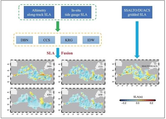
4.1. The Capability of Describing the Spatial Characteristics

Through the above three-step experiment and comparison, the results indicate that SLA estimation based on the DBN method is more feasible and robust than the other three traditional methods. Furthermore, regarding the capability of each method to describe the spatial characteristics of fused SLAs, using training scheme (b), the SLAs were fused in January 2002 and January 2012 with a spatial resolution of 0.25° × 0.25° as shown in Figure 7. Additionally, keeping the selected tide gauges for external control unchanged in scheme (b), the 20% randomly sampled Jason-1/2-derived along-track SLAs were substituted by all the along-track SLAs as the additional training data to evaluate the precision of CCS and the DBN, and the results are shown in Figure 7 with notes for CCS+ and DBN+. All these fused SLAs were compared with the gridded SLA product provided by SSALTO/DUACS, which is merged with multi-satellite altimetry data using the optimal interpolation method.
From Table 4 and Figure 7, using a better external control with evenly distributed tide gauges in scheme (b), the spatial characteristics of the four methods are diverse. Compared with the SLAs using optimal interpolation with multi-altimetry data, the result for the DBN shows the most details and has the best agreement, while the result of KRG shows fewer details, and the result of CCS shows more details than that of IDW. Theoretically, the more altimetry-derived SLAs are used as training data, the more spatial change details can be captured by fusion methods. From Figure 7, it can be seen that the improvement of CCS is limited, but that of the DBN model is significant, showing more consistency with the result of optimal interpolation with multi-altimetry data. That is to say, the DBN method is not only able to improve the precision of SLA time series estimation but is also capable of capturing more spatial characteristics than the other three methods.

4.2. Other Potential Deep Learning Methods

The DBN model is not the only deep learning method, and other methods may be introduced and compared in the future. Such as the long-short term memory (LSTM) network [40] and the temporal convolutional network (TCN) [41,42].
The LSTM network performs exceptionally well in analyzing time-series data. It has a significant advantage over the traditional recurrent neural network, the forget gate, which determines what information is discarded from cellular state. Sun et al. [43] combined the seasonal autoregressive integrated moving average (SARIMA) model and a LSTM model to increase the sea level prediction accuracy, and the performance was superior in predicting sea level changes with a minimum root mean square error of 1.155 cm and a maximum determination coefficient of 0.89 during the testing period. Fan et al. [44] compared the LSTM significant wave height prediction results with that from a back propagation neural network, extreme learning machine, support vector machine, residual network, and random forest algorithm. The results demonstrated that the LSTM can achieve stable prediction effects, with accurate 1-h predictions and satisfactory 6-h predictions. Liu et al. [45] proposed a LSTM network-based SLA Intelligent Inversion model to fit the SLA model based on the traditional gravest empirical mode (GEM) field and the relative error of network was less than 0.15% when compared with traditional GEM.
A general architecture for a predictive sequences model by convolutional and recurrent architecture on sequence modeling tasks, the TCN, was proposed in recent year [41,42]. The typical characteristics of TCN includes: (1) It can take a sequence of any length and output it as a sequence of the same length with the input, just like using a recurrent neural network; and (2) the convolution is a causal convolution, which means that there is no information “leakage” from future to past. Based on TCN, Hewage et al. [46] developed a novel and location specific weather forecasting system. The experiments showed that the model using TCN produced better forecasting compared to other classic machine learning approaches. As the El Niño-Southern Oscillation (ENSO) prediction accuracy of current popular numerical methods was not high, Yan et al. [47] proposed an ensemble empirical mode decomposition and TCN hybrid approach to obtain ENSO prediction results and the correlation coefficient between the worst predicted southern oscillation index and the actual value reached 0.64.
The successful applications of the LSTM network and the TCN in these studies indicate that maybe they can be used to fuse satellite altimetry and tide gauge observations as they consider time dependence. In future research, the LSTM- or TCN-based SLA fusion method will be developed and assessed.

5. Conclusions

In this study, a deep learning method, the DBN model, was used to fuse altimetry and tide-gauge-derived SLAs. Taking the Mediterranean Sea as the case study and using the IDW, KRG and CCS methods for comparison, a progressive experiment was designed to evaluate the precision of the DBN method on SLA fusion. The results indicate that DBN method is more adaptable and stable than the other three methods. With the altimetry-derived along-track SLAs and in-situ tide gauge observed SLAs, the precision of the DBN method was verified to be approximately 20% higher than the others in the different distributions of control tide gauge data, especially when the quantity of control tide gauges was limited and their spatial distribution was uneven. Furthermore, the precision of the DBN model was certified to be less affected than the other methods by the distribution of training data from altimetry-derived SLAs (gridded or along-track). Most importantly, the fused SLAs of the DBN model had more spatial details and were more consistent with the results of optimal interpolation with multi-altimetry data.
Due to the limitations of satellite altimetry, a high-quality unified sea level model from coast to open ocean has traditionally been difficult to achieve, even when waveform retracking is used to improve the accuracy of altimetry-derived sea level in the near-shore areas. On the other hand, with the development of multi-techniques, there are a growing number of new observation technologies (such as GNSS-R) in-situ sea level measurements, so it is necessary to fuse these accumulated data with altimeter sea levels to generate more useful and reliable unified SLAs. After comparison with several commonly used methods, it was proven that deep learning can be applied as a more feasible and robust way to reduce the fusion gaps and gain more spatial details, especially when the external condition is inadequate and complex.

Author Contributions

T.J. conceived the experiment process, wrote the revised version of the paper; L.Y. realized the deep learning method, made further processing of experiment data and analysis, and wrote the initial version of paper; M.X. helped to analyze the traditional methods; X.G. made initial processing of the along-track altimeter data; H.W., T.S. and H.H. helped on the analysis and revision. All authors have read and agreed to the published version of the manuscript.

Funding

This research was funded by National Natural Science Foundation of China under Grants 41721003 and 41974020; The Major Project of High-resolution Earth Observation System under Grants 42-Y20A09-9001-17/18; DAAD Thematic Network Project under Grant 57173947; National Key R&D Program of China under Grant 2016YFB0501702.

Data Availability Statement

The tide gauge data is provided by PSMSL (http://www.psmsl.org/data/obtaining/ (accessed on 15 January 2021)). The gridded global mean sea level anomalies product is provided by AVISO (https://www.aviso.altimetry.fr/en/data/products/sea-surface-height-products/global.html (accessed on 15 January 2021)). The Jason-1 and Jason-2 data is achieved from Radar Altimeter Database System (http://rads.tudelft.nl/rads/ (accessed on 15 January 2021)). The GNSS vertical land motions are available from SONEL (https://www.sonel.org (accessed on 15 January 2021)) and the EUREF Permanent Network (http://www.epncb.oma.be/_productsservices/coordinates/ (accessed on 15 January 2021)).

Acknowledgments

All the respectable reviewers and editors are acknowledged for their fruitful comments and suggestions about the paper.

Conflicts of Interest

The authors declare no conflict of interest.

References

  1. Church, J.A.; White, N.J. A 20th century acceleration in global sea-level rise. Geophys. Res. Lett. 2006, 33. [Google Scholar] [CrossRef]
  2. Kirezci, E.; Young, I.R.; Ranasinghe, R.; Muis, S.; Nicholls, R.J.; Lincke, D.; Hinkel, J. Projections of global-scale extreme sea levels and resulting episodic coastal flooding over the 21st Century. Sci. Rep. 2020, 10, 11629. [Google Scholar] [CrossRef] [PubMed]
  3. Bonaduce, A.; Pinardi, N.; Oddo, P.; Spada, G.; Larnicol, G. Sea-level variability in the Mediterranean Sea from altimetry and tide gauges. Clim. Dyn. 2016, 47, 2851–2866. [Google Scholar] [CrossRef] [Green Version]
  4. Nerem, R.S.; Mitchum, G.T. Estimates of vertical crustal motion derived from differences of TOPEX/POSEIDON and tide gauge sea level measurements. Geophys. Res. Lett. 2002, 29, 40–44. [Google Scholar] [CrossRef]
  5. Kuo, C.Y.; Shum, C.K.; Braun, A.; Miteovica, J.X. Vertical crustal motion determined by satellite altimetry and tide gauge data in Fennoscandia. Geophys. Res. Lett. 2004, 31. [Google Scholar] [CrossRef] [Green Version]
  6. Schöne, T.; Schön, N.; Thaller, D. IGS Tide Gauge Benchmark Monitoring Pilot Project (TIGA): Scientific benefits. J. Geod. 2009, 83, 249–261. [Google Scholar] [CrossRef]
  7. Gharineiat, Z.; Deng, X. Application of the Multi-Adaptive Regression Splines to Integrate Sea Level Data from Altimetry and Tide Gauges for Monitoring Extreme Sea Level Events. Mar. Geod. 2015, 38, 261–276. [Google Scholar] [CrossRef]
  8. Avsar, N.B.; Jin, S.; Kutoglu, H.; Gurbuz, G. Sea level change along the Black Sea coast from satellite altimetry, tide gauge and GPS observations. Geod. Geodyn. 2016, 7, 50–55. [Google Scholar] [CrossRef] [Green Version]
  9. Taibi, H.; Haddad, M. Estimating trends of the Mediterranean Sea level changes from tide gauge and satellite altimetry data (1993–2015). J. Oceanol. Limnol. 2019, 37, 1176–1185. [Google Scholar] [CrossRef]
  10. Grgić, M.; Nerem, R.S.; Bašić, T. Absolute Sea Level Surface Modeling for the Mediterranean from Satellite Altimeter and Tide Gauge Measurements. Mar. Geod. 2017, 40, 239–258. [Google Scholar] [CrossRef]
  11. Hinton, G.E.; Osindero, S.; Teh, Y.-W. A fast learning algorithm for deep belief nets. Neural Comput. 2006, 18, 1527–1554. [Google Scholar] [CrossRef] [PubMed]
  12. Fu, Y.; Aldrich, C. Flotation froth image recognition with convolutional neural networks. Miner. Eng. 2019, 132, 183–190. [Google Scholar] [CrossRef]
  13. Liu, N.; Xu, Y.; Tian, Y.; Ma, H.; Wen, S. Background classification method based on deep learning for intelligent automotive radar target detection. Future Gener. Comput. Syst. 2019, 94, 524–535. [Google Scholar] [CrossRef]
  14. Du, Y.; Song, W.; He, Q.; Huang, D.; Liotta, A.; Su, C. Deep learning with multi-scale feature fusion in remote sensing for automatic oceanic eddy detection. Inf. Fusion 2019, 49, 89–99. [Google Scholar] [CrossRef] [Green Version]
  15. Ducournau, A.; Fablet, R. Deep learning for ocean remote sensing: An application of convolutional neural networks for super-resolution on satellite-derived SST data. In Proceedings of the 2016 9th IAPR Workshop on Pattern Recogniton in Remote Sensing (PRRS), Cancun, Mexico, 4 December 2016; pp. 1–6. [Google Scholar]
  16. Braakmann-Folgmann, A.; Roscher, R.; Wenzel, S.; Uebbing, B.; Kusche, J. Sea Level Anomaly Prediction using Recurrent Neural Networks. arXiv 2017, arXiv:1710.07099. [Google Scholar]
  17. Bruneau, N.; Polton, J.; Williams, J.; Holt, J. Estimation of global coastal sea level extremes using neural networks. Environ. Res. Lett. 2020, 15, 074030. [Google Scholar] [CrossRef]
  18. Zhu, S.-B.; Li, Z.-L.; Zhang, S.-M.; Ying, Y.; Zhang, H.-F. Deep belief network-based internal valve leakage rate prediction approach. Measurement 2019, 133, 182–192. [Google Scholar] [CrossRef]
  19. Wang, H.Z.; Wang, G.B.; Li, G.Q.; Peng, J.C.; Liu, Y.T. Deep belief network based deterministic and probabilistic wind speed forecasting approach. Appl. Energy 2016, 182, 80–93. [Google Scholar] [CrossRef]
  20. Huang, H.B.; Li, R.X.; Yang, M.L.; Lim, T.C.; Ding, W.P. Evaluation of vehicle interior sound quality using a continuous restricted Boltzmann machine-based DBN. Mech. Syst. Signal Process. 2017, 84, 245–267. [Google Scholar] [CrossRef] [Green Version]
  21. Ji, H.; Tian, L.; Li, J.; Tong, R.; Guo, Y.; Zeng, Q. Spatial-spectral Fusion of HY-1C COCTS/CZI Data for Coastal Water Remote Sensing Using Deep Belief Network. IEEE J. Sel. Top. Appl. Earth Obs. Remote Sens. 2020. [Google Scholar] [CrossRef]
  22. Li, T.; Shen, H.; Yuan, Q.; Zhang, X.; Zhang, L. Estimating Ground-Level PM2.5 by Fusing Satellite and Station Observations: A Geo-Intelligent Deep Learning Approach. Geophys. Res. Lett. 2017, 44, 11, 985–911, 993. [Google Scholar] [CrossRef] [Green Version]
  23. Krige, D.G. A statistical approach to some basic mine valuation problems on the Witwatersrand. J. South Afr. Inst. Min. Metall. 1951, 52, 119–139. [Google Scholar]
  24. Smith, W.; Wessel, P. Gridding with continuous curvature splines in tension. Geophysics 1990, 55, 293–305. [Google Scholar] [CrossRef]
  25. Ducet, N.; Le Traon, P.Y.; Reverdin, G. Global high-resolution mapping of ocean circulation from TOPEX/Poseidon and ERS-1 and -2. J. Geophys. Res. Ocean. 2000, 105, 19477–19498. [Google Scholar] [CrossRef]
  26. AVISO. SSALTO/DUACS User Handbook: (M) SLA and (M) ADT Near-Real Time and Delayed Time Products; CNES: Ile-de-France, France, 2014. [Google Scholar]
  27. Scharroo, R.; Leuliette, E.; Lillibridge, J.; Byrne, D.; Naeije, M.; Mitchum, G. RADS: Consistent multi-mission products. In Proceedings of the 20 Years of Progress in Radar Altimatry, Venice, Italy, 24–29 September 2012. [Google Scholar]
  28. Holgate, S.J.; Matthews, A.; Woodworth, P.L.; Rickards, L.J.; Tamisiea, M.E.; Bradshaw, E.; Foden, P.R.; Gordon, K.M.; Jevrejeva, S.; Pugh, J. New Data Systems and Products at the Permanent Service for Mean Sea Level. J. Coast. Res. 2012, 29, 493–504. [Google Scholar] [CrossRef]
  29. Santamaría-Gómez, A.; Gravelle, M.; Wöppelmann, G. Long-term vertical land motion from double-differenced tide gauge and satellite altimetry data. J. Geod. 2014, 88, 207–222. [Google Scholar] [CrossRef]
  30. Bruyninx, C.; Habrich, H.; Söhne, W.; Kenyeres, A.; Stangl, G.; Völksen, C. Enhancement of the EUREF permanent network services and products. In Geodesy for planet Earth; Springer: Berlin/Heidelberg, Germany, 2012; pp. 27–34. [Google Scholar]
  31. Carrère, L.; Lyard, F. Modeling the barotropic response of the global ocean to atmospheric wind and pressure forcing-comparisons with observations. Geophys. Res. Lett. 2003, 30. [Google Scholar] [CrossRef] [Green Version]
  32. Wöppelmann, G.; Marcos, M. Coastal sea level rise in southern Europe and the nonclimate contribution of vertical land motion. J. Geophys. Res. Ocean. 2012, 117. [Google Scholar] [CrossRef] [Green Version]
  33. Shen, H.; Li, T.; Yuan, Q.; Zhang, L. Estimating Regional Ground-Level PM2. 5 Directly From Satellite Top-Of-Atmosphere Reflectance Using Deep Belief Networks. J. Geophys. Res. Atmos. 2018, 123, 13, 875–813, 886. [Google Scholar] [CrossRef] [Green Version]
  34. Yuan, Q.; Shen, H.; Li, T.; Li, Z.; Li, S.; Jiang, Y.; Xu, H.; Tan, W.; Yang, Q.; Wang, J. Deep learning in environmental remote sensing: Achievements and challenges. Remote Sens. Environ. 2020, 241, 111716. [Google Scholar] [CrossRef]
  35. Mohamed, A.-R.; Dahl, G.E.; Hinton, G. Acoustic modeling using deep belief networks. IEEE Trans. Audio Speech Lang. Process. 2011, 20, 14–22. [Google Scholar] [CrossRef]
  36. Chen, Z.; Li, W. Multisensor Feature Fusion for Bearing Fault Diagnosis Using Sparse Autoencoder and Deep Belief Network. IEEE Trans. Instrum. Meas. 2017, 66, 1693–1702. [Google Scholar] [CrossRef]
  37. Kingma, D.P.; Ba, J. Adam: A method for stochastic optimization. arXiv 2014, arXiv:1412.6980. [Google Scholar]
  38. Smolensky, P. Information Processing in Dynamical Systems: Foundations of Harmony Theory; Colorado University at Boulder Department of Computer Science: Boulder, CO, USA, 1986. [Google Scholar]
  39. Hinton. A Practical Guide to Training Restricted Boltzmann Machines. In Neural Networks: Tricks of the Trade; Springer: Berlin/Heidelberg, Germany, 2012; pp. 599–619. [Google Scholar]
  40. Hochreiter, S.; Schmidhuber, J. Long Short-Term Memory. Neural Comput. 1997, 9, 1735–1780. [Google Scholar] [CrossRef] [PubMed]
  41. Bai, S.; Kolter, J.Z.; Koltun, V. An empirical evaluation of generic convolutional and recurrent networks for sequence modeling. arXiv 2018, arXiv:1803.01271. [Google Scholar]
  42. Lea, C.; Flynn, M.D.; Vidal, R.; Reiter, A.; Hager, G.D. Temporal Convolutional Networks for Action Segmentation and Detection. In Proceedings of the IEEE Conference on Computer Vision and Pattern Recognition, Honolulu, HI, USA, 21–26 July 2017; pp. 156–165. [Google Scholar]
  43. Sun, Q.; Wan, J.; Liu, S. Estimation of sea level variability in the China Sea and its vicinity using the SARIMA and LSTM models. IEEE J. Sel. Top. Appl. Earth Obs. Remote Sens. 2020, 13, 3317–3326. [Google Scholar] [CrossRef]
  44. Fan, S.; Xiao, N.; Dong, S. A novel model to predict significant wave height based on long short-term memory network. Ocean Eng. 2020, 205, 107298. [Google Scholar] [CrossRef]
  45. Liu, H.; He, B.; Qin, P.; Zhang, X.; Guo, S.; Mu, X. Sea level anomaly intelligent inversion model based on LSTM-RBF network. Meteorol. Atmos. Phys. 2020, 1–15. [Google Scholar] [CrossRef]
  46. Hewage, P.; Behera, A.; Trovati, M.; Pereira, E.; Ghahremani, M.; Palmieri, F.; Liu, Y. Temporal convolutional neural (TCN) network for an effective weather forecasting using time-series data from the local weather station. Soft Comput. 2020, 24, 16453–16482. [Google Scholar] [CrossRef] [Green Version]
  47. Yan, J.; Mu, L.; Wang, L.; Ranjan, R.; Zomaya, A.Y. Temporal convolutional networks for the advance prediction of ENSO. Sci. Rep. 2020, 10, 1–15. [Google Scholar] [CrossRef]
Figure 1. The distribution of initial tide gauge stations (blue dots) and GNSS stations (red triangles).
Remotesensing 13 00908 g001
Figure 2. The structure of the SLA estimation model based on DBN method.
Remotesensing 13 00908 g002
Figure 3. The distribution of training data (red) and validation data (blue) without tide gauges (a), and the correlation coefficients (b), RMSE (c) and STD (d) for four methods. The horizontal coordinates of (bd) are percentages of gridded SLAs (%).
Remotesensing 13 00908 g003
Figure 4. The correlation coefficients (a,d), RMSE (b,e) and STD (c,f) of the four methods with virtual tide gauges.
Remotesensing 13 00908 g004
Figure 5. The distribution of altimetry-derived SLAs in the training data (blue dots) and the in-situ tide gauge training data (blue triangles) as well as validation data (red dots) in schemes (a,b).
Remotesensing 13 00908 g005
Figure 6. The distribution of in-situ tide gauges used as external control for different schemes and altimetry-derived along-track SLAs in training data. Scheme (b) is shown in Figure 5; scheme (c) in Table 3 is not shown; scheme (g) represents no tide gauge selected as external control.
Remotesensing 13 00908 g006
Figure 7. The spatial characteristics of the fused SLAs in January 2002 (A) and January 2012 (B) from KRG (d), CCS (b,c), DBN (e,f) and IDW (g) methods, as well as the product from SSALTO/DUACS (a).
Remotesensing 13 00908 g007
Table 1. Statistics of the four methods with altimetry-derived gridded SLAs in schemes (a) (m).
Tide Gauge
Number
DBNCCSKRGIDW
CORRSTDRMSECORRSTDRMSECORRSTDRMSECORRSTDRMSE
3 0.877 0.040 0.040 0.914 0.036 0.044 0.862 0.043 0.053 0.820 0.048 0.059
6 0.796 0.038 0.038 0.652 0.046 0.064 0.781 0.038 0.052 0.785 0.037 0.052
7 0.872 0.041 0.041 0.846 0.045 0.056 0.843 0.045 0.057 0.810 0.049 0.061
8 0.939 0.024 0.025 0.775 0.043 0.056 0.811 0.040 0.053 0.800 0.041 0.054
10 0.790 0.039 0.039 0.643 0.047 0.065 0.759 0.040 0.053 0.769 0.039 0.053
11 0.904 0.034 0.034 0.895 0.037 0.048 0.879 0.039 0.052 0.832 0.044 0.057
12 0.893 0.032 0.034 0.866 0.035 0.049 0.857 0.036 0.049 0.861 0.035 0.050
13 0.943 0.023 0.025 0.775 0.043 0.057 0.824 0.039 0.052 0.823 0.039 0.052
17 0.859 0.038 0.040 0.838 0.041 0.055 0.842 0.041 0.054 0.847 0.040 0.053
18 0.933 0.025 0.028 0.833 0.035 0.049 0.825 0.036 0.049 0.833 0.035 0.048
19 0.922 0.029 0.031 0.855 0.040 0.050 0.865 0.039 0.049 0.848 0.041 0.051
20 0.901 0.037 0.037 0.852 0.045 0.060 0.862 0.044 0.058 0.846 0.047 0.060
21 0.886 0.050 0.051 0.846 0.057 0.064 0.833 0.059 0.068 0.798 0.064 0.073
24 0.864 0.038 0.039 0.765 0.047 0.055 0.772 0.046 0.057 0.769 0.046 0.057
Mean0.884 0.035 0.036 0.811 0.043 0.055 0.830 0.042 0.054 0.817 0.043 0.056
Table 2. Statistics of the four methods with altimetry-derived along-track SLAs in scheme (b) (m).
Tide Gauge
Number
DBNCCSKRGIDW
CORRSTDRMSECORRSTDRMSECORRSTDRMSECORRSTDRMSE
3 0.869 0.041 0.041 0.859 0.034 0.034 0.866 0.042 0.043 0.813 0.049 0.050
6 0.883 0.029 0.029 0.737 0.036 0.056 0.836 0.033 0.034 0.812 0.036 0.037
7 0.860 0.043 0.043 0.844 0.042 0.044 0.853 0.044 0.046 0.855 0.044 0.046
8 0.929 0.025 0.026 0.802 0.041 0.048 0.794 0.041 0.045 0.797 0.041 0.044
10 0.908 0.026 0.026 0.835 0.040 0.041 0.865 0.031 0.032 0.833 0.034 0.035
11 0.892 0.036 0.036 0.872 0.039 0.040 0.846 0.042 0.044 0.804 0.047 0.048
12 0.881 0.033 0.034 0.826 0.039 0.042 0.859 0.035 0.038 0.862 0.035 0.038
13 0.933 0.025 0.025 0.865 0.034 0.041 0.811 0.040 0.044 0.816 0.039 0.043
17 0.857 0.038 0.039 0.835 0.041 0.044 0.853 0.039 0.042 0.858 0.039 0.042
18 0.916 0.027 0.029 0.843 0.035 0.038 0.846 0.035 0.036 0.839 0.035 0.037
19 0.907 0.032 0.034 0.909 0.030 0.031 0.896 0.034 0.034 0.875 0.036 0.037
20 0.886 0.040 0.040 0.755 0.055 0.061 0.814 0.050 0.053 0.800 0.051 0.054
21 0.868 0.054 0.054 0.829 0.054 0.054 0.848 0.057 0.059 0.788 0.065 0.067
24 0.870 0.036 0.037 0.791 0.046 0.048 0.793 0.044 0.049 0.790 0.045 0.050
Mean0.890 0.035 0.035 0.829 0.040 0.044 0.841 0.040 0.043 0.824 0.043 0.045
Table 3. Details of the six schemes of external control tide gauges.
SchemeTG Stations Used as Training DataSpatial Distribution Characteristics
b[ 1,2,4,5,9,14,15,16,22,23]Evenly distributed
c[ 2,3,4,6,8,14,17,20,21,24]Evenly distributed
d[ 2,11,12,14,16,17,18,19,20,22]Inside
e[ 1,3,5,6,7,8,9,10,13,15,21]Upper left corner
f[ 4,12,14,17,18,19,22,23,24]Bottom right corner
g[ ]No tide gauge is selected
Table 4. Statistics of the four methods in six schemes with altimetry-derived along-track SLAs (m).
SchemeDBNCCSKRGIDW
CORRSTDRMSECORRSTDRMSECORRSTDRMSECORRSTDRMSE
b0.890 0.035 0.035 0.829 0.040 0.044 0.841 0.040 0.043 0.824 0.043 0.045
c0.907 0.031 0.032 0.859 0.034 0.036 0.853 0.038 0.040 0.844 0.039 0.041
d0.863 0.039 0.040 0.776 0.052 0.057 0.793 0.047 0.050 0.786 0.047 0.050
e0.885 0.036 0.037 0.817 0.047 0.050 0.820 0.044 0.047 0.821 0.044 0.047
f0.846 0.042 0.042 0.765 0.056 0.062 0.763 0.050 0.052 0.758 0.050 0.052
g0.861 0.039 0.040 0.761 0.052 0.057 0.786 0.047 0.050 0.785 0.047 0.050
Mean0.875 0.037 0.038 0.801 0.047 0.051 0.809 0.044 0.047 0.803 0.045 0.047
Publisher’s Note: MDPI stays neutral with regard to jurisdictional claims in published maps and institutional affiliations.

