
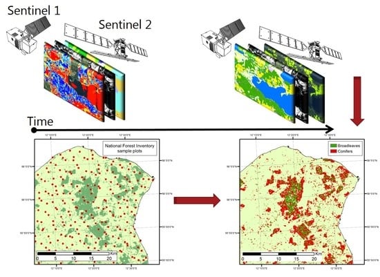
Classification of Nemoral Forests with Fusion of Multi-Temporal Sentinel-1 and 2 Data


1
SLA, 2300 Copenhagen S, Denmark
2
Department of Geosciences and Natural Resource Management (IGN), University of Copenhagen, 1958 Frederiksberg C, Denmark
*
Author to whom correspondence should be addressed.
Remote Sens. 2021, 13(5), 950; https://0-doi-org.brum.beds.ac.uk/10.3390/rs13050950
Submission received: 11 January 2021
/
Revised: 23 February 2021
/
Accepted: 25 February 2021
/
Published: 3 March 2021
(This article belongs to the Special Issue Forest Monitoring in a Multi-Sensor Approach)
Abstract
:Mapping forest extent and forest cover classification are important for the assessment of forest resources in socio-economic as well as ecological terms. Novel developments in the availability of remotely sensed data, computational resources, and advances in areas of statistical learning have enabled the fusion of multi-sensor data, often yielding superior classification results. Most former studies of nemoral forests fusing multi-sensor and multi-temporal data have been limited in spatial extent and typically to a simple classification of landscapes into major land cover classes. We hypothesize that multi-temporal, multi-sensor data will have a specific strength in the further classification of nemoral forest landscapes owing to the distinct seasonal patterns in the phenology of broadleaves. This study aimed to classify the Danish landscape into forest/non-forest and further into forest types (broadleaved/coniferous) and species groups, using a cloud-based approach based on multi-temporal Sentinel 1 and 2 data and a random forest classifier trained with National Forest Inventory (NFI) data. Mapping of non-forest and forest resulted in producer accuracies of 99% and 90%, respectively. The mapping of forest types (broadleaf and conifer) within the forested area resulted in producer accuracies of 95% for conifer and 96% for broadleaf forest. Tree species groups were classified with producer accuracies ranging 34–74%. Species groups with coniferous species were the least confused, whereas the broadleaf groups, especially Quercus species, had higher error rates. The results are applied in Danish national accounting of greenhouse gas emissions from forests, resource assessment, and assessment of forest biodiversity potentials.
1. Introduction
Forests produce a wide range of socio-economic goods for the owners of forest lands as well as for the surrounding society. Many of these goods are closely related to the spatial distribution of forests and tree species. Different tree species are managed differently, may be used for producing different products, and are sold at different prices yielding widely different economic profiles for the forest owner. In relation to climate change, different species accumulate different amounts of carbon in widely different temporal patterns [1], thereby contributing differently to climate change mitigation. The interception and evaporation of precipitation in tree crowns differ between tree species and results in different rates of ground water formation as well as in different ground water quality [2,3,4]. Furthermore, different forest tree species produce different habitats and therefore contribute differently to biodiversity conservation in general [5]. The future provision of the goods provided by forests are largely dependent on their spatial arrangement, since different tree species will be affected differently by climate change, depending on complex interactions with the local site conditions as well as with other trees [6].
Due to the intrinsic relationship between the spatial forest and forest tree species distribution and the provision of socio-economic goods, mapping of forests and forest tree species provide a possibility to assess the provision of such goods. Consequently, mapping of forests as part of management planning has been detailed and widely used since the beginning of the 19th century [7]. However, previous methods of forest resource mapping were time consuming, expensive, and hardly feasible in today’s society. Meeting the society’s needs for detailed and at the same time cost-effective mapping of forest characteristics based on remote sensing (RS) commenced in the early 1970s [8] and began a rapid development in the mapping of forest ecosystem services, including forest resources [9,10,11,12,13], carbon storage [14,15], biological diversity [16,17,18], habitats [19,20,21], and forest recreation [22].
In recent decades, the possibility to map forests and forest tree species distributions has increased dramatically due to improvements in the temporal and spatial resolution of remotely sensed data, the combination of multiple sensor systems, increasing processing capacity as well as advances in areas of statistical learning. A prominent feature of recent advances in classification is the fusion of multi-sensor data [23,24,25]. Different sensors vary in terms of spatial and temporal resolution as well as in the properties of data collected. Therefore, combining different sensors may overcome shortcomings of individual sensors, providing improved classification results [26].
A vast number of studies have used the fusing of various sources of RS data for different aspects of land use and land cover classification [27,28]. In an analysis including 32 studies reviewing the advantages of fusing optical and radar data for land use analysis, the vast majority concluded that the fusion of RS data improved forest classification compared to using a single source [29]. The fusion of data from different sensor systems may provide means to characterize other elements of the forest environment. For example, combining multispectral images containing specific reflectance attributes of plants and Light Detection and Ranging (LiDAR) data providing understanding of structural canopy properties may be used for characterizing forest habitats [30,31,32], while the combination of synthetic aperture radar (SAR) and LiDAR may yield accurate estimates of biophysical quantities, such as biomass [33].
Adding a temporal dimension, the fusion of multi-temporal acquisitions of RS data provide opportunities to detect changes in, for example, forest cover over time [34]. However, in the nemoral forest zone, multi-temporal data may further detect seasonal variation in spectral signature and radiometric backscatter specific to e.g., individual tree species or forest types. With a common denominator of detecting seasonal changes in spectral signatures, several studies have used multi-temporal data for mapping forest types, growing stocks or habitats [35,36,37,38,39]. However, until recently, factors unrelated to forest properties such as weather and ground conditions caused anomalies in annual signal variations, inhibiting applications such as land cover typing [40].
In recent years, the high acquisition frequencies of dual synthetic aperture radar (SAR) Sentinel-1 (S-1) and optical Sentinel-2 (S-2) has provided novel opportunities for the classification of forested landscapes from multi-temporal data. In a study aiming to classify deciduous and coniferous forests as well as individual species in Switzerland, multi-temporal S-1 C-band backscatter was applied for the classification of forest types and tree species [41]. In this study, a timespan of only 24 days between individual composites from January 2015 to May 2017 was used to observe seasonal changes in backscatter related to phenotypical changes in foliage. The study clearly demonstrated seasonal changes in vertical–horizontal (VH) backscatter for both forest types; coniferous forests had stronger backscatter in summer and lower at the end of winter, whereas deciduous forests showed the opposite trend. Similar behavior was observed for individual species, although differences were less pronounced between the two broadleaved species. The temporal changes in backscatter were instrumental in obtaining high accuracies in the classification of forest types with the random forest classifier (OA = 0.86) and clearly demonstrated the advantages of using multi-temporal data for the classification of nemoral forests. Similarly, Dostalova et al. [40] performed forest area estimation and forest type classification in the nemoral (Austria) and boreal (Sweden) zone, resting on the assumption that S-1 time series data would produce a distinct seasonal backscatter signature aiding the differentiation of vegetation types. The study demonstrated that high accuracies in the classification of forest types were possible in the nemoral zone, yielding an overall accuracy of 0.85, whereas the accuracy dropped to 0.65 in the boreal zone. This was attributed to the lack of seasonal variation of leaf-cover in the boreal zone, underpinning the underlying rationale for using multi-temporal data in the classification.
A novel but intuitive step from multi-sensor and multi-temporal approaches to classification is expanding the concept to include both multi-sensor and multi-temporal data. A study aiming to map forest–agriculture mosaics across highly different landscapes in Spain and Brazil by combining multi-temporal sets of S-1 and S-2 with a random forest classifier demonstrated that overall, the combination of sensors increased accuracy compared to those obtained from the single sensors [42]. However, the study also demonstrated differences in the number and types of features that yielded superior classification depending on the landscape considered. This indicates that the combination of multi-temporal data from several sensors may yield results that are more consistent across a range of landscapes. Supporting this notion, a study using a similar combination of multi-temporal S-1 and S-2 data for forest/non-forest classification in Germany and South Africa yielded overall accuracies exceeding 0.90 in both landscapes [43]. The combination of sensors with a random forest classifier yielded robust results and was superior to using the single sensors only. Expanding the concept even further, a study on the classification of eight different forest types in Wuhan, China included both mono-temporal S-1, S-2, and digital elevation (DEM) data and multi-temporal Landsat-8 data [44]. As in the other studies, the highest overall accuracy (0.83) was obtained when fusing data from several sensors. This effort demonstrates that the use of multi-temporal and multi-sensor data consistently performs well across a wide range of landscapes and classification tasks.
Most former studies conducted on nemoral forest resources were limited in spatial extent and/or focused on a simple classification of landscapes into major land cover classes. However, we hypothesize that multi-temporal, multi-sensor data will have a specific strength in the further classification of nemoral forest landscapes into forest types or even individual species owing to the distinct seasonal patterns of the phenology of nemoral broadleaved forests. Based on this notion, this study aims to classify the Danish landscape (43,000 km2) into forest/non-forest and further into forest types (broadleaved/coniferous) and species groups. This is achieved by the semi-automatic classification of multi-temporal S-1 and S-2 images using a random forest classifier trained with samples from the National Forest Inventory (NFI).
2. Materials and Methods
The presented methodology comprises the preprocessing of multi-temporal S-1 and S-2 data from the Copernicus Programme, the acquisition of suitable reference information from the National Forest Inventory (NFI), and machine learning-based model building and classification including performing tuning and validation procedures.
To get a representation of the main phenological changes in the landscape during a year, two sets of image composites were created; a set representing the winter period after the senescence of deciduous trees and a set representing the summer period after the foliation of deciduous trees. A summary of all 33 feature layers included in the models and their mean and standard deviation is provided in Appendix Table A1. All initial pre-processing of satellite images were performed in the Google Earth Engine (GEE) code environment [45] (see Section 2.1 and Section 2.2).
2.1. Preparation of Optical Data
Multispectral optical features were generated from a series of S-2 Level-2A BOA (bottom-of-atmosphere) satellite images covering the study area. The Level-2A BOA products were generated from Level-1C TOA (top-of-atmosphere) images using the Sen2Cor processor [46]. According to a study of the atmospheric correction accuracy, root mean square error (RMSE) between Sen2Cor BOA reflectance and in situ measurements ranges from 0.002 to 0.005 [47]. After the activation of the Global Reference Image (GRI) geometric refinement, the geometric accuracy of S-2 multi-temporal co-registration is now better than 0.3 pixel (at 2σ confidence level) [48]. The winter collection of optical images comprised a series of 1325 S-2 images acquired on 118 distinct dates between 1 November 2018 and 27 February 2019, while the summer collection comprised a series of 1381 S-2 images acquired on 121 distinct days between 15 May and 14 September 2019.
The cloud-masking and compositing procedures suggested by Hird et al. [49] were applied to produce per-pixel, cloud-free multispectral composites for the winter and summer period, respectively. The procedure includes identifying and masking out flagged cloud and cirrus pixels based on the S-2 Band QA60 as well as the application of a Band 1 threshold cut-off of ≥1500 to mask out remaining clouds and aerosols. With the applied two-stage procedure of masking and mosaicking of dense temporal image collections, we minimized the risk of cloud-covered pixels in the final composites. Further to this end, true-color (RGB) composites of the area of interest were visually inspected for any obvious cloud or haze issues.
The normalized difference vegetation index (NDVI) was calculated for all images and added to the set. Finally, a cloud-free composite of each spectral band and the NDVI covering the entire land surface of Denmark was derived by applying a median compositing function on the winter and summer images, respectively. The median composite function removes any anomalous dark pixels (shadows) as well as bright, saturated pixels. All bands with a resolution of 10–20 m were selected, including bands within the visible (band 2–4), near infrared (NIR, band 5–8), and short wave infrared (SWIR, band 10–12) parts of the electromagnetic spectrum. The 20 m resolution bands were resampled (nearest neighbor) to 10 m resolution, and all 22 feature layers (11 winter and 11 summer composites) were exported as GeoTif-files.
To add a textural component to the image set, seven rotation-invariant Haralick texture features were calculated and added using a 3 × 3 window on the NDVI summer composite, including mean, variance, homogeneity, contrast, dissimilarity, entropy, and second moment [50].
2.2. Preparation of SAR Data
SAR features were generated from a series of C-band S-1 Level-1 Ground Range Detected images with a pixel size of 10 m. Each S-1 frame had a size of 29,600 × 21,900 pixels. The data were recorded in Interferometric Wide swath mode (IW), with incidence angels between 30 and 45 degrees (both ascending and descending) and delivered in dual polarization, both vertical–vertical (VV) and vertical–horizontal (VH). The images were pre-processed using the S-1 Toolbox [51], including thermal noise removal, radiometric calibration, and terrain correction.
The winter collection comprised a series of 554 S-1 images acquired on 119 distinct dates between 1 November 2018 to 26 February 2019, while the summer collection comprised a series of 513 S-1 images acquired on 123 distinct days between 15 May and 13 September 2019. The images in each collection (summer and winter) were mosaicked to a composite for each of the two polarizations (VV and VH) of the area of interest by applying a mean function on the winter and summer collection, respectively. The final four composite images (two summer and two winter composites) were smoothened with a 3 × 3 window mean filter and exported as GeoTif files.
2.3. National Forest Inventory Data
Sample plot measurements from the Danish National Forest Inventory (NFI) were applied as ground-truth reference data for training of the classifiers and validation of the classification output. The NFI is a sample-based inventory with a partial replacement of sample plots and is carried out on a yearly basis [52]. The sample plots are structured in a 2 × 2 km grid covering the whole country. Each sample plot (viz. primary sampling units or PSU for short) is composed of four circular subplots (viz. secondary sampling units or SSU for short) with a radius of 15 m and centered on the corners of a 200 × 200 m square. A total of ≈43,000 SSUs are included in the sampling design but only a representative subsample of 1/5 covering the entire country is measured every year of a 5-year cycle. Prior to each year’s measurements, the presence/absence of forest within SSU is identified on the most recent aerial photographs (typically updated every year, [53]), and only forest covered plots are measured in the field. The SSU may be subdivided into tertiary sampling units (TSU), when covering several land use classes or forest stands.
The SSUs are located in the field using a Trimble GPS Pathfinder Pro XRS receiver mounted with a Trimble Hurricane antenna. The precision of the equipment is expected to be sub-one meter. The SSUs have a nested design composed of three concentric circles with a radius of 3.5, 10, and 15 m respectively. In the 3.5-m circle, the diameter of all trees is measured (single calipered) at breast height (1.3 m). In the 10-m circle, trees with a diameter >10 cm are measured, and only trees with a diameter >40 cm are measured on the full SSU. Total height is measured on a random sample of 2–6 trees inside the plot. Further recordings of relevance for this study include the registration of tree species and crown cover. The crown cover in percent is estimated visually on temporary SSUs (2/3 of the sample) and using a densiometer on permanent SSUs (1/3 of the sample). Total crown cover is aggregated as the area weighted average of the TSU level estimates.
The individual SSU is designated a forest type (broadleaf, conifer, or mixed) based on the proportion of the basal area of the measured trees. If broadleaves represent more than 75% of the basal area, the plot is characterized as broadleaf and vice versa for conifers. If these criteria are not met, the plot is characterized as mixed forest.
Preparation of NFI Data
The forest definition applied in the NFI follows the definition of the Global Forest Resource Assessment [54], i.e., a minimum area of 0.5 ha wider than 20 m with a minimum crown cover of 10% with trees with a minimum height of 5 m. The definition includes areas where the vegetation has the potential of reaching the aforementioned criteria as well as temporarily unstocked areas and permanently unstocked areas designated to forest management. The definitions exclude areas dominated by agricultural or urban land uses such as orchards, cottage areas, and city parks.
The use of NFI sample plots for the pixel-based classification of remotely sensed imagery may be problematic when labeling is obtained from the 706 m2 large circular sample plots, but the classification is subsequently trained and evaluated on 100 m2 (10 × 10 m) pixels [55]. In this case, the labeling obtained from the entire plot may not apply to the individual pixels encompassed (i.e., when one sample plot spans several land cover classes), leading to poorer training of the classifier. This is contrasting the common practice of selecting a statistical sample for classification or evaluation from an already classified map commonly derived from data with similar or finer resolution than the resulting map, where all pixels may be uniquely classified [56]. To reduce ambiguity at the pixel level in the reference data, a stricter definition of forest was applied, aiming to reduce instances were pixels may be wrongly labeled e.g., for SSUs only partly covered by forest. Consequently, an SSU was labeled as forest if more than 75% was characterized as forest and with a crown cover of more than 10%. An SSU was labeled as non-forest if 0% of the plot was characterized as forest and the estimated crown cover equals 0%. SSUs falling between these thresholds were labeled as ambiguous and removed from the reference data (Table 1).
Similar to the classification of forest cover, the overall labeling of forest types obtained from the NFI plots may, in the case of mixed forests, not adhere to the smaller individual pixels within the plot. Individual tree crowns may exceed the pixel-size used in our study, and hence, pixels will commonly represent one particular forest type rather than the mixture of species present on the NFI plot. Since the spatial arrangement of tree crowns within the plots is unknown, we had no possibility to correct the classification of individual pixels within the plot. Consequently, for classification into forest types (conifer/broadleaf), only SSUs either dominated by coniferous or broadleaved species respectively, (i.e., constituting a basal area of more than 75% of the plot) were included in the reference data (Table 1). All other SSUs were disregarded in the analysis.
For tree species classification, six distinct classes were defined based on the morphological similarities and prevalence in the Danish forest area. A class can both consist of a single predominant species, a genus, or ensembles of minor important species grouped together. Hereafter, species, genera, and species groups are referred to as tree species. The six classes include the following:
(1) Fagus, comprising European beech (Fagus sylvatica).
(2) Quercus, comprising pedunculate oak (Quercus robur), sessile oak (Quercus petaea), and red oak (Quercus rubra).
(3) Other broadleaves, comprising European ash (Fraxinus excelsior), birch (Betula sp.), sycamore maple (Acer pseudoplatanus), as well as broadleaves of minor importance such as alder (Alnus sp.), willow (Salix sp.), and hornbeam (Carpinus betulus).
(4) Picea, comprising Norway spruce (Picea abies) and Sitka spruce (Picea sitchensis).
(5) Pinus, comprising Scotts pine (Pinus sylvestris) as wells as minor important pine species such as Austrian pine (Pinus nigra) and mountain pine (Pinus mugo ssp. mugo).
(6) Other conifers, comprising species of fir (Abies sp.), Douglas fir (Pseudotsuga menziesii), as well as conifers of miner importance such as western red cedar (Thuja plicata) and Lawson cypress (Chamaecyparis lawsoniana).
As for forest type classification, only SSUs that were dominated (>75% of basal area) by one of the species of the defined classes were included in the reference data.
The training dataset was restricted to SSUs measured in the field season of 2018 to reduce the temporal span between field measurements and image acquisition, resulting in a total of 8586 SSUs. Post classification, erroneous classification caused by the temporal displacement between field measurements and image acquisition, i.e., when changes in canopy cover occurred between data collections, was detected manually from high-resolution aerial images [53]. Plots where changes occurred between data acquisitions were removed and the classification process was iteratively re-run. Only a very limited number of forest plots were subject to change between time of acquisition and measurement.
The training data were created by stacking all 33 input layers (both optical and SAR) into one raster brick and subsequently sampling all band values from pixels with a centroid covered by a 10-m circular buffer of every labeled SSU center coordinate. This resulted in a total of 24,584 (corresponding to an average of three pixel samples per SSU), 2220, and 1812 pixel samples for forest cover classification, tree type classification, and species classification, respectively.
The evaluation data were based on SSUs measured in the field seasons of 2017 and 2019 keeping the maximum temporal span between the field data collection and the recording of satellite images at approximately one year and avoiding spatial correlation with the training data. The evaluation dataset included a total of 17,020 reference SSUs.
2.4. Model Building and Evaluation Framework
The three different classification tasks (forest cover, forest type, and tree species) were performed in a hierarchical procedure. First, the forest area was delineated by the forest cover classification model. Secondly and thirdly, the delineated forest mask was classified into forest type (conifer-/broadleaf-dominated) and tree species. In all cases, the output was in 10 × 10 m resolution.
To escape rigid assumptions regarding model form and issues with overfitting related to the often large number of variables involved, we applied the non-parametric Random Forest (RF) algorithm [57] for the supervised classification of pixels. The RF classifier is a decision tree-based ensemble classifier, building on the idea of bagging. Bagging applies bootstrapping, i.e., iteratively resampling with replacement of the original reference dataset, to create a collection of candidate decision trees, which are then aggregated by majority vote. Each decision tree extends from the roots to leaves under a set of conditions and restrictions. The roots represent the full variation of the sample and the leaves represent the terminal nodes (i.e., the final number of classes). At each node within the tree, a randomly selected subset of predictors available are considered for binary splitting into decisions based on a decision rule. From the user-defined number of trees (the “forest”), classification decision is based on the most popular voted class from all the decision trees in the forest to stabilize predictions, reduce bias, and avoid overfitting.
RF differs from ordinary bagging by using a random subset of the total amount of predictors available when constructing the individual trees. The randomness in feature selection helps de-correlate the individual trees, thereby improving the variance reduction introduced by the bagging procedure. The relatively few assumptions attached to RF make data preparation and model parameterization less challenging. Consequently, RF has been applied successfully for a variety of remote sensing-based forestry applications [58,59,60,61].
Model tuning and training of the RF classifiers were performed in the CARET package in R [62]. The models were trained on all 33 input features (Table A1) without prior scaling and with no restrictions on tree depth. The hyper-parameters were tuned using resampling by repeated 10-fold cross-validation to stabilize predictions and were optimized with respect to the overall accuracy (OA). The optimal settings of the hyper-parameters, i.e., the number of trees and the number of variables to be selected and tested for the best split when growing the trees, may vary between the individual classifiers and are reported in the results section for each of the three classifiers.
To estimate the area proportions of the mapped land cover classes and the corresponding standard errors, a “good practice” workflow for error-adjusted area estimation was subsequently applied [63]. This involves the use of confusion matrix information in which the accuracy assessment of individual classes provides information on the magnitude of the classification errors that allows an adjustment to be made in the area estimator [64].
The classification performance was evaluated based on the independent evaluation dataset by the confusion matrix including overall accuracy (OA) as well as producer’s (PA) and user’s accuracy (UA) for the different classes. Feature importance was analyzed using a RF-based wrapper algorithm implemented in the Boruta package in R [65]. The algorithm works by creating permuted copies of the included features called shadow features. Subsequently, an RF classifier is trained with respect to the response of interest on the extended set of features, and the importance measured in mean decrease accuracy is logged for every feature. Each feature is iteratively checked against the best performing shadow feature in terms of Z-score and either rejected or confirmed based on the relative importance. The algorithm was configured to perform 1000 iterations.
2.5. Post Classification Filtering
To close part of the gap between the land-use definition of forest comprised by the NFI and the strict land cover definition used in the classification, two post-classification filtering procedures were applied. To comply with the minimum mapping unit criteria of the NFI, all clusters of coherent forest pixels less than 50 corresponding to an area of 0.5 ha was masked out. To comply with at least some of the land-use criteria in the NFI, areas mapped as low build-up in the GeoDanmark mapping [66] were masked out. The low build-up polygons include amongst others cottage areas, gardens, playgrounds, lawns, parks, and parking lots.
3. Results
3.1. Forest Cover Model
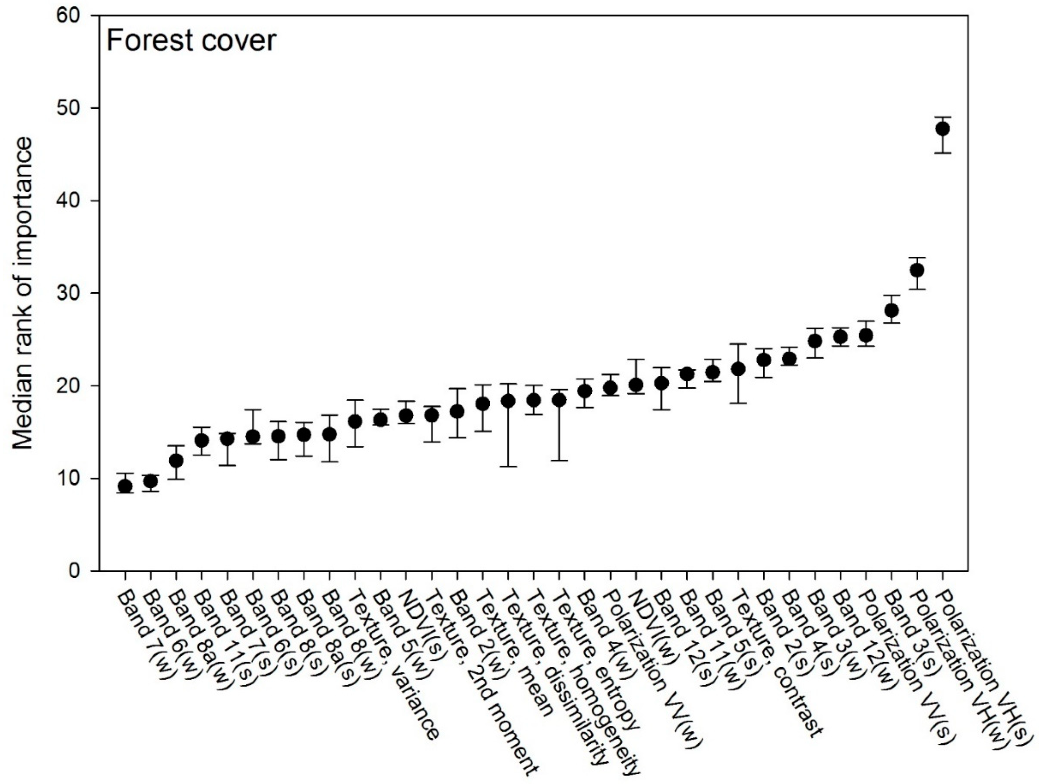
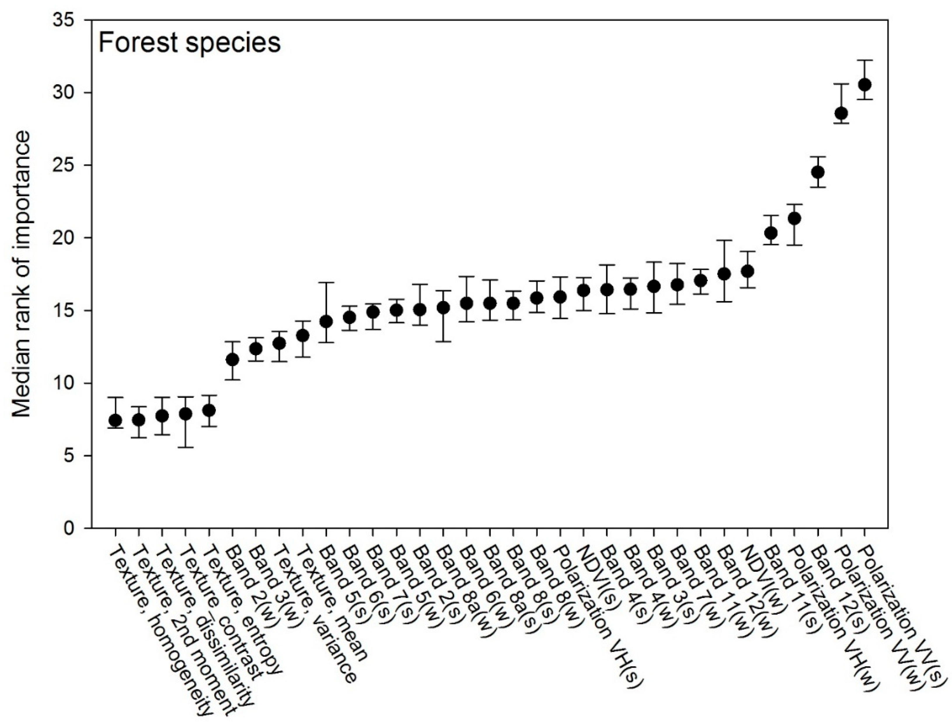
The training procedure for the RF classification of forest cover resulted in 500 trees and seven splitting features per tree node. Based on the Boruta simulations, all 33 input features were significant when classifying forest and non-forest (Figure 1). The most important features in predicting forest cover were the summer and winter SAR images in VH polarization (VHs and VHw). The most important features of the optical data were the green band of the summer composite (B3s) and the SWIR band of the winter composite (B12w). In general, the most important features for classification of forest/non-forest were obtained from the S-1 SAR images (three out of the four most important features). When considering the individual types of data (i.e., optical bands, SAR polarizations, etc.), the summer image was nearly always more important for the classification than the winter image. Textural features from the optical data were shown to have a moderate importance when using classification forest vs. non-forest.
The forest mapping resulted in an overall accuracy of 98%, with a 99% correct classification of non-forest (PA) and a 90% correct classification of forest (PA) (Figure 2, Table 2). Producer and user accuracies were fairly balanced, indicating that errors of commission/omission were in the same order of magnitude. The raw forest cover mapping resulted in a forest area of 637,290 ha (±10,402 ha) corresponding to a forest fraction of 14.8%. Adjusting the area estimate by the classification errors in accordance with the “good practice” workflow for error-adjusted area estimation only changed the forest proportion marginally, yielding a forest area of 638,750 ha.
The raw forest cover map was post-processed by the application of the minimum mapping unit (MMU) filter removing forest areas of less than 0.5 ha and low build-up filter removing cottage areas, gardens, playgrounds, lawns, etc. After filtering, the mapping resulted in 100% correct classification of non-forest and a 90% correct classification of forest (Table 2). The resulting map reported a forest area of 597,980 ha (±8573) corresponding to a forest fraction of 13.9%. The error-adjusted estimate was 636,079 ha corresponding to a forest fraction of 14.8%.
3.2. Forest Type Model
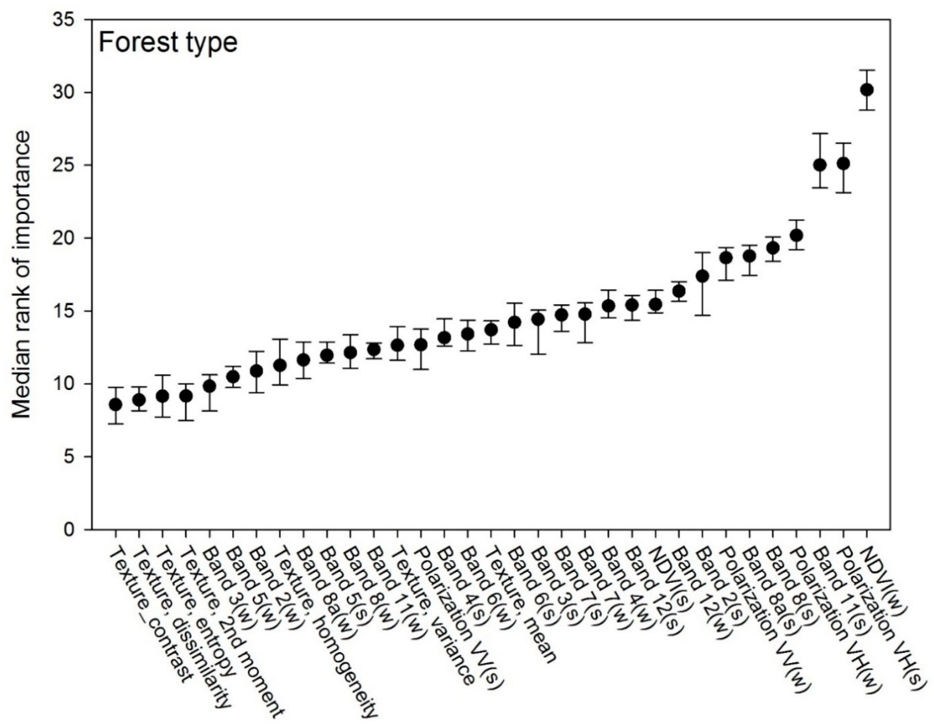
For the forest type classification, the RF model training resulted in 500 trees and 11 splitting features per tree node. Based on the Boruta simulations, all 33 input features were found to be significant (Figure 3). The most important feature in predicting tree type was the winter NDVI image (NDVIw) followed by the SAR VH polarization summer image (VHs) and the band 11 SWIR summer image (B11s). The SAR VH polarization winter image (VHw) comes out as the fourth most important feature. When considering the individual type of data, the summer image was in most cases markedly more important for the classification than the winter image. Most of the textural features were less important for this type of classification.
The mapping of forest types (broadleaf and conifer) resulted in an overall accuracy of 95% in the correct classification of 95% (PA) of conifer and 96% (PA) of broadleaf forest (Table 3). As for the forest vs. non-forest classification, the forest type classification revealed a balanced level of commission/omission errors. The estimated conifer forest area adjusted for classification errors was 268,824 ha (±7247 ha), corresponding to a fraction 45.0% of the forest area. The adjusted broadleaf forest area was estimated to 329,156 ha (±7247 ha), corresponding to 55.0% of the forest area.
3.3. Tree Species Model
The training of the RF tree species classification model resulted in 500 trees and four splitting features per tree node. Based on the Boruta simulations, all 33 input features were found to be significant. The most important feature in predicting tree species was the summer SAR image in VV polarization (VVs) followed by the winter VV image (VVw) and the band 12 SWIR summer image (B12s) (Figure 4). The SAR VH polarization winter image (VHw) is shown to be the fourth most important feature. As for the other classifications, the S-1 SAR features were generally important for the classification of individual species, but we found no particular pattern in the importance of summer vs. winter features for the classification. As for the forest type model, the textural features from the optical imagery were less important for the species type classification.
The tree species were classified with an overall accuracy of 63%. Producer accuracies were ranging from 34% to 73% (Table 4), with the Quercus species showing noticeable lower accuracies than the remaining species and the Pinus species performed the best. The species groups consisting of coniferous species were the least confused, whereas the broadleaf groups (especially Quercus species) had a higher error rate. The error-adjusted estimated area proportions and their confidence intervals are reported in Table 4.
4. Discussion
4.1. Forest Cover Classification
Our study demonstrated that the use of multi-temporal data combining optical and SAR data from S-1 and S-2 led to very high classification accuracies of forest/non-forest. We found the overall most important features for classifying forest cover to be the S-1 VH polarization (summer and winter composite). The total backscatter from a forest at wavelengths of 5.6 cm (C-band) comes primarily from leaves or needles and twigs of the upper canopy and their interactions, allowing the identification of forest/non-forest areas [67,68]. The importance of the dual-polarization (VH) information over single-polarization (VV) for non-forest vs. forest cover classification aligns well with the well-known higher sensitivity of VH microwave backscatter to total above-ground biomass than VV [68]. The importance of VH information over spectral signatures from optical instruments for forest extent mapping contrasts other studies fusing S-1 and S-2 data, who have found optical data features from the S-2 to be superior in areas covering temperate dense mixed forests, open savanna woody vegetation, and forest plantations as well as forest–agriculture mosaics [42,43]. However, Heckel et al. [43] found that S-1 SAR data were better at predicting tree cover in highly fragmented landscapes, which apply to the intensively cultivated Danish landscape. It is well known that SAR-derived land cover classification is imposed by topographic relief, and here, the flat terrain of all Danish landscapes makes an ideal case for optimal signal-to-noise in the use of S-1 data. The highest ranking S-2 optical features were Band 3 (green) summer composite and Band 12 (SWIR) winter composite, which were also amongst the top predictors in [43].
The total forest area resulting from the final map was very close to the forest area of 598,186 ha (excluding unstocked areas) reported by the Danish NFI [69] with a deviation of less than 0.1%. A comparison of the mapped forest area to the land use map resulting from the national emissions inventory [70] demonstrated that the differences mainly included temporarily unstocked forest and auxiliary areas included in the forest definition such as fire breaks, forest roads, etc.
The obtained accuracies for the forest cover classification correspond to a mapping accuracy similar to that obtained in other studies using combinations of S-1 and S-2 data [42] and to the accuracy obtained for land classification with multi-seasonal Landsat Thematic Mapper-5 images [71]. The accuracy obtained in our study should be viewed in the context of the small-scale variation typical for the Danish landscape but also recognizing that we in this study distinguished only between forest and non-forest, where the studies above distinguished between up to eight different land cover types. Even higher accuracies of classifying only forest/non-forest (OA = 99%) were obtained in relation to a study of forest type classification in Wuhan, China when fusing S-2 and DEM images obtained from the Shuttle Radar Topography Mission (SRTM) [44]. In countries with very small differences in elevation, such as Denmark where the highest point is 171 m a.s.l., it is unlikely that the inclusion of a DEM would improve classification results. However, wall-to-wall airborne laser scanning campaigns in Denmark have provided canopy height models, which in future efforts could be used to improve forest/non-forest classification [72].
4.2. Forest Type Classification
The classification of the forested landscape into forest types (i.e., broadleaved and coniferous forest) had similar classification accuracy to the forest/non-forest classification with an overall of accuracy of 95%. Not surprisingly, given the phenological differences between the two forest types, NDVI obtained from winter images had the highest mean rank of importance among the variables used in the classification. The use of dual-polarization SAR data (VH) was also found to perform well in discriminating between broadleaved and coniferous forests, which is likely caused by the intrinsic nature of SAR backscatter responding to the structure of the forest (forest-type specific volume scattering from different interaction with leaves versus needles and twigs of the upper canopy).
The classification accuracy of forest types obtained in this study was higher than that obtained in a study by Dostálová, et al. [40], reporting an overall accuracy of 85% when classifying the forest type (between non-forest, coniferous, and broadleaf forest classes) in temperate forest from the use of multi-temporal S-1 only. In their study, the VH polarization was found to contain most of the information necessary to perform a forest-type classification. In a study by Rüetschi et al. [41], an overall accuracy of 86% was achieved in classifying deciduous and coniferous species, using S-1 in Northern Switzerland. Other studies of forest type classification with the fusion of images from different sensors include the classification of eight different forest types in Wuhan, China from multiple sources of RS data including S-1, S-2, DEM, and Landsat 8 images [44] and the classification of 11 subtropical forest types in Guangxi Zhuang, China from ZiYuan-3, S-2, and Landsat 8 images [73]. In the study by Liu et al. [44], the highest accuracy (83%) was achieved when using the fusion of S-2, DEM, S-1 (VV polarization), and Landsat 8 images, and the authors concluded that that elevation and multi-temporal data contributed the most to forest type identification. Similarly, Yu et al. [73] found the highest classification accuracy (84%) when using both spectral and topographical data. As with the classification of forest/non-forest, it is unlikely that the inclusion of terrain differences would improve classification results in a flat country, such as Denmark, as also observed by Strahler et al. [74]. However, as with the classification of forest/non-forest, airborne laser scanning in Denmark has provided canopy height models that may provide additional information relevant to the classification of forest types [72].
The resulting forest type distribution was very similar to that obtained from the Danish NFI (51% broadleaved forest and 49% conifer forest) [69]. Some of the differences between observed and predicted forest type was due to misclassification of larch (≈1% of the forest area [69]), which was likely due to phenological changes across seasons similar to broadleaves.
4.3. Tree Species Classification
Our classification of individual tree species showed lower accuracy than the classification of forest types with an overall accuracy of 63% and producer accuracies ranging 34–74% for individual species and species groups. The features of highest importance for the classification of tree species in the nemoral forests in our study were primarily the S-1 SAR images in VV polarization obtained during summer and winter, contrasting the classification of forest and forest type, where the SAR images in VH polarization performed better. The obtained accuracy was lower than the one obtained in a much similar study using multi-temporal optical S-2 images for species classification in Central Sweden [75]. Using four S-2 from April, May, June, and October, Persson et al. [75] reported an overall accuracy of 88% for the area-based classification of five different tree species. The most important classifiers in the study op. cit. included the red edge bands 2 and 3 as well as the narrow NIR (near-infrared) band 8a, which were all obtained on 27 May.
Although we found a different set of potential variables to be more important in the classification, we speculate that higher species classification accuracy may generally be obtained if including several images around the time of flushing of the nemoral species in April–June and during the peak of autumn colors in October–November. The possibility for successfully doing so depends on the cloud cover during this critical time of the growing cycle. Another option would be to make use of the full temporal resolution of the S-1 and S-2 data to produce per-pixel phenological metrics such as start, end, and length of growing season that have otherwise proven useful in land cover classification [76,77,78]. Other approaches for the classification of single tree species are typically based on remote sensing data sources (LiDAR and other very high resolution (VHR) data) not currently offered as cloud-based date sources facilitating national-scale wall-to-wall coverage analysis of no cost [79,80] or the fusion of S-2 data and Airborne Laser Scanning data [81].
Noticeably, in our study, the groups of conifers were more accurately classified than the broadleaves. Especially, Quercus species were poorly classified. We speculate that the differences in results may be related to differences in crown size, as also pointed out in a comprehensive review on tree species classification from remotely sensed data [82]. In the predominant management systems in Denmark, Quercus species are often open grown and obtain large crowns compared to most conifers commonly managed with dense stocking to avoid wind throw. With a pixel size of 10 m in the present study, each pixel may cover several conifer crowns, but for older trees of Quercus and Fagus, they cover less than a tree crown. Another feature of Quercus species management that may affect the result is the common use of understory crops to prevent the formation of epicormics branches, which may influence the reflected radiation from other trees [83,84], which is often too small to be captured by the design of NFI plots.
Finally, in our study, species groups were formed with respect to the prevalence of the individual species and their seeming similarities rather than based on a study of their spectral reflectance. We believe that improvements to the classification would be possible if forming species groups based on an analysis of similarities in spectral reflectance for different tree species such as those presented by Persson et al. [75].
4.4. Use of NFI Data in Area-Based Classification
A prominent feature of our study was the use of NFI sample plots (0.0706 ha) covering all land cover classes across the entire country area for both training and as reference in the evaluation of prediction accuracy. The classification of the individual plots into forest/non-forest relies on a visual interpretation of high-resolution (12.5 cm pixel-size) aerial photographs, which is subsequently validated for all plots with possible forest or other wooded land (OWL) cover. The subsequent classification of forested land into forest types and tree species relied on manual measurements of the trees inside the plot. This approach contrasts most other studies, commonly using existing maps or manual discrimination of polygons from aerial photographs [42,43,71] or the classification of coarse resolution pixels from high-resolution RS data [85].
Our choice of reference features a number of advantages over alternative approaches. The sample was freely available and collected in accordance with established and internationally acknowledged procedures [86]. Furthermore, the sample available for training is large, unbiased, and represents the entire landscape rather than small test sites as often the case in similar studies [82]. Finally, the information available on the individual plots has a high degree of accuracy based on actual field measurements. However, the NFI design also posed a number of challenges when used for area-based mapping of forest cover. Although the Danish NFI use a sample plot size larger than most countries [86], the sample plots often cover more than one land use, forest type, and tree species. We elected to discard sample plots if a contrasting class covered more than 25% of the sample area, and although this approach may be practical, it inevitably reduces the samples and ignore obvious variability. Another issue is related to the use of concentric circles for measuring different size trees. Individual sample plots may be dominated by tree crowns of trees that are not measured when they are placed outside the concentric circle in which they should be measured. It is likely that some of the explanation for the poor performance of tree species classification is related to this issue.
5. Conclusions
In this study, we used freely available multi-source data for wall-to-wall classification of the Danish forest landscape using Google Earth Engine (GEE) cloud computing and a Random Forest machine-learning classifier. Substantiating previous research, the fusion of multi-temporal and multi-sensor Sentinel 1 and 2 data yielded robust estimates with high accuracies of both forest/non-forest and forest type classification. However, the classification of individual tree species performed less well and remains the most challenging classification task within nemoral forest landscape inventorying. With reference to studies on classification with hyper-temporal data, we suggest future studies to increase the temporal depth in the Sentinel 1 and 2 data usage, which might overcome this limitation of our study by better capturing distinct seasonal patterns in the spectral signature of the nemoral tree species. A prominent feature of our study was the use of National Forest Inventory (NFI) data for labeling pixels used to train and evaluate the classification algorithm. The NFI data provided an unbiased sample covering the entire domain, controlled in the field, and readily available to the user. However, plots with ambiguous land cover or tree species characteristics posed a specific challenge in relation to labeling samples for the training and validation of the Sentinel 1 and 2-based classification, representing a smaller mapping unit (10 m resolution) than the NFI data. We recommend that future research be devoted to handling the often equivocal labeling of the reference sample with particular reference to NFI sample plots, which provide unparalleled opportunities for cost-efficient bridging of the gap between point-based estimates obtained from the NFI and local to national scale wall-to-wall estimates of forest landscapes relevant to e.g., forest owners and administers.
Author Contributions
Conceptualization, K.S.B., T.N.-L.; methodology, K.S.B., T.N.-L., R.F.; software, K.S.B.; validation, K.S.B., T.N.-L.; formal analysis, K.S.B.; investigation, K.S.B., T.N.-L.; resources, K.S.B., T.N.-L.; data curation, K.S.B.; writing—original draft preparation, K.S.B., T.N.-L.; writing—review and editing, K.S.B., T.N.-L., R.F.; visualization, K.S.B.; supervision, T.N.-L.; project administration, T.N.-L.; funding acquisition, T.N.-L. All authors have read and agreed to the published version of the manuscript.
Funding
This research received no external funding.
Institutional Review Board Statement
Not applicable.
Informed Consent Statement
Not applicable.
Data Availability Statement
Not applicable.
Conflicts of Interest
The authors declare no conflict of interest. The funders had no role in the design of the study; in the collection, analyses, or interpretation of data; in the writing of the manuscript, or in the decision to publish the results.
Appendix A

Table A1.
Feature layers included in the models and their mean and standard deviation. All features except the texture features comes in a summer (s) and a winter (w) version.
Table A1.
Feature layers included in the models and their mean and standard deviation. All features except the texture features comes in a summer (s) and a winter (w) version.
| Layer (Summer/Winter) | Abbreviations (Features) | Mean (Summer) | Stdv (Summer) | Mean (Winter) | Stdv (Winter) |
|---|---|---|---|---|---|
| Optical data | |||||
| Raw electromagnetic bands (BOA reflectance value x 10,000) | |||||
| Band 2 | B2s/B2w | 493.49 | 179.88 | 531.34 | 156.43 |
| Band 3 | B3s/B3w | 725.78 | 205.71 | 622.60 | 190.95 |
| Band 4 | B4s/B4w | 590.64 | 266.30 | 543.47 | 220.51 |
| Band 5 | B5s/B5w | 1131.30 | 279.24 | 1008.45 | 278.03 |
| Band 6 | B6s/B6w | 2583.70 | 593.68 | 1958.57 | 802.36 |
| Band 7 | B7s/B7w | 3097.74 | 745.61 | 2214.70 | 923.49 |
| Band 8 | B8s/B8w | 3257.64 | 798.44 | 2398.27 | 994.51 |
| Band 8A | B8As/B8Aw | 3374.79 | 788.27 | 2418.02 | 946.46 |
| Band 11 | B11s/B11w | 1807.18 | 449.32 | 1484.68 | 436.14 |
| Band 12 | B12s/B12w | 1027.51 | 369.10 | 925.03 | 308.94 |
| Vegetation index | |||||
| Normalized Difference Vegetation Index | NDVIs/NDVIw | 0.65 | 0.17 | 0.57 | 0.20 |
| Haralick Texture features (only on NDVIs) | |||||
| Mean | - | 0.86 | 0.09 | - | - |
| Variance | - | 721.16 | 140.91 | - | - |
| Homogeneity | - | 0.76 | 0.17 | - | - |
| Dissimilarity | - | 0.56 | 0.51 | - | - |
| Contrast | - | 1.07 | 1.71 | - | - |
| Entropy | - | 1.08 | 0.60 | - | - |
| Second moment | - | 0.45 | 0.27 | - | - |
| SAR data (Radar image reflectance values) | |||||
| Vertical-Vertical polarization | VVs/VVw | −10.84 | 2.40 | −10.36 | 2.42 |
| Vertical-Horizontal polarization | VHs/VHw | −17.51 | 2.59 | −18.19 | 2.99 |
References
- Nord-Larsen, T.; Pretzsch, H. Biomass production dynamics for common forest tree species in Denmark—Evaluation of a common garden experiment after 50 years of measurements. For. Ecol. Manag. 2017, 400, 645–654. [Google Scholar] [CrossRef]
- Rothe, A. Tree Species Management and Nitrate Contamination of Groundwater: A Central European Perspective. In Tree Species Effects on Soils: Implications for Global Change; Springer: Dordrecht, The Netherlands, 2005; pp. 71–83. [Google Scholar]
- Salazar, O.; Hansen, S.; Abrahamsen, P.; Hansen, K.; Gundersen, P. Water Balance in Afforestation Chronosequences of Common Oak and Norway Spruce on Former Arable Soils in Denmark as Evaluated Using the DAISY Model. Procedia Environ. Sci. 2013, 19, 217–223. [Google Scholar] [CrossRef] [Green Version]
- Christiansen, J.R.; Vesterdal, L.; Callesen, I.; Elberling, B.; Schmidt, I.K.; Gundersen, P. Role of six European tree species and land-use legacy for nitrogen and water budgets in forests. Glob. Chang. Biol. 2010, 16, 2224–2240. [Google Scholar] [CrossRef]
- Quine, C.P.; Humphrey, J.W. Plantations of exotic tree species in Britain: Irrelevant for biodiversity or novel habitat for native species? Biodivers. Conserv. 2010, 19, 1503–1512. [Google Scholar] [CrossRef]
- Dyderski, M.K.; Paź, S.; Frelich, L.E.; Jagodziński, A.M. How much does climate change threaten European forest tree species distributions? Glob. Chang. Biol. 2018, 24, 1150–1163. [Google Scholar] [CrossRef]
- Loetsch, F.; Haller, K. Forest Inventory; BLV Verlagsgesellschaft: München, Germany, 1964; Volume I. [Google Scholar]
- Roth, W.; Olson, C. Multispectral Sensing of Forest Tree Species. Photogramm. Eng. 1972, 38, 1209–1215. [Google Scholar]
- Boyd, D.; Danson, F. Satellite remote sensing of forest resources: Three decades of research development. Prog. Phys. Geogr. 2005, 29, 1–26. [Google Scholar] [CrossRef]
- Nord-Larsen, T.; Schumacher, J. Estimation of forest resources from a country wide laser scanning survey and national forest inventory data. Remote Sens. Environ. 2012, 119, 148–157. [Google Scholar] [CrossRef]
- Næsset, E.; Gobakken, T.; Holmgren, J.; Hyyppä, H.; Hyyppä, J.; Maltamo, M.; Nilsson, M.; Olsson, H.; Persson, Å.; Söderman, U. Laser scanning of forest resources: The Nordic experience. Scand. J. For. Res. 2004, 19, 482–499. [Google Scholar] [CrossRef]
- Næsset, E. Practical large-scale forest stand inventory using a small-footprint airborne scanning laser. Scand. J. For. Res. 2004, 19, 164–179. [Google Scholar] [CrossRef]
- Næsset, E. Accuracy of forest inventory using airborne laser scanning: Evaluating the first nordic full-scale operational project. Scand. J. For. Res. 2004, 19, 554–557. [Google Scholar] [CrossRef]
- Akujärvi, A.; Lehtonen, A.; Liski, J. Ecosystem services of boreal forests—Carbon budget mapping at high resolution. J. Environ. Manag. 2016, 181, 498–514. [Google Scholar] [CrossRef] [PubMed]
- Mononen, L.; Vihervaara, P.; Repo, T.; Korhonen, K.T.; Ihalainen, A.; Kumpula, T. Comparative study on biophysical ecosystem service mapping methods—A test case of carbon stocks in Finnish Forest Lapland. Ecol. Ind. 2017, 73, 544–553. [Google Scholar] [CrossRef]
- Lehtomäki, J.; Tomppo, E.; Kuokkanen, P.; Hanski, I.; Moilanen, A. Applying spatial conservation prioritization software and high-resolution GIS data to a national-scale study in forest conservation. For. Ecol. Manag. 2009, 258, 2439–2449. [Google Scholar] [CrossRef]
- Räsänen, A.; Lensu, A.; Tomppo, E.; Kuitunen, M. Comparing Conservation Value Maps and Mapping Methods in a Rural Landscape in Southern Finland. Landsc. Online 2015, 44, 1–21. [Google Scholar] [CrossRef]
- Johannsen, V.K.; Rojas, S.K.; Brunbjerg, A.K.; Schumacher, J.; Bladt, J.; Nyed, P.K.; Moeslund, J.E.; Nord-Larsen, T.; Ejrnæs, R. Udvikling af et High. Nature Value—HNV-Skovkort for Danmark; Institut for Geovidenskab og Naturforvaltning, Københavns Universitet: Frederiksberg, Denmark, 2015. [Google Scholar]
- Vatka, E.; Kangas, K.; Orell, M.; Lampila, S.; Nikula, A.; Nivala, V. Nest site selection of a primary hole-nesting passerine reveals means to developing sustainable forestry. J. Avian Biol. 2014, 45. [Google Scholar] [CrossRef]
- McDermid, G.J.; Franklin, S.E.; LeDrew, E.F. Remote sensing for large-area habitat mapping. Prog. Phys. Geogr. 2005, 29, 449–474. [Google Scholar] [CrossRef]
- McDermid, G.J.; Hall, R.J.; Sanchez-Azofeifa, G.A.; Franklin, S.E.; Stenhouse, G.B.; Kobliuk, T.; LeDrew, E.F. Remote sensing and forest inventory for wildlife habitat assessment. For. Ecol. Manag. 2009, 257, 2262–2269. [Google Scholar] [CrossRef]
- Jusoff, K.; Hassan, H.M. Forest recreation planning in Langkawi Island, Malaysia, using landsat TM. Int. J. Remote Sens. 1996, 17, 3599–3613. [Google Scholar] [CrossRef]
- Wolter, P.P.; Townsend, P.A. Multi-sensor data fusion for estimating forest species composition and abundance in northern Minnesota. Remote Sens. Environ. 2011, 115, 671–691. [Google Scholar] [CrossRef]
- Fortin, J.A.; Cardille, J.A.; Perez, E. Multi-sensor detection of forest-cover change across 45 years in Mato Grosso, Brazil. Remote Sens. Environ. 2020, 238, 111266. [Google Scholar] [CrossRef]
- Lu, M.; Chen, B.; Liao, X.; Yue, T.; Yue, H.; Ren, S.; Li, X.; Nie, Z.; Xu, B. Forest Types Classification Based on Multi-Source Data Fusion. Remote Sens. 2017, 9, 1153. [Google Scholar] [CrossRef] [Green Version]
- Poortinga, A.; Tenneson, K.; Shapiro, A.; Nquyen, Q.; San Aung, K.; Chishtie, F.; Saah, D. Mapping Plantations in Myanmar by Fusing Landsat-8, Sentinel-2 and Sentinel-1 Data along with Systematic Error Quantification. Remote Sens. 2019, 11, 831. [Google Scholar] [CrossRef] [Green Version]
- Zhang, J. Multi-source remote sensing data fusion: Status and trends. Int. J. Image Data Fusion 2010, 1, 5–24. [Google Scholar] [CrossRef] [Green Version]
- Mahyouba, S.; Fadilb, A.; Mansour, E.; Rhinanea, H.; Al-Nahmia, F. Fusing of optical and synthetic aperture radar (SAR) remote sensing data: A systematic literature review (SLR). Int. Arch. Photogramm. Remote Sens. Spat. Inf. Sci. 2019, 42, 127–138. [Google Scholar] [CrossRef] [Green Version]
- Joshi, N.; Baumann, M.; Ehammer, A.; Fensholt, R.; Grogan, K.; Hostert, P.; Jepsen, M.R.; Kuemmerle, T.; Meyfroidt, P.; Mitchard, E.T.A.; et al. A Review of the Application of Optical and Radar Remote Sensing Data Fusion to Land Use Mapping and Monitoring. Remote Sens. 2016, 8, 70. [Google Scholar] [CrossRef] [Green Version]
- Asner, G.P.; Martin, R.E.; Anderson, C.B.; Knapp, D.E. Quantifying forest canopy traits: Imaging spectroscopy versus field survey. Remote Sens. Environ. 2015, 158, 15–27. [Google Scholar] [CrossRef]
- Martin, R.E.; Chadwick, K.D.; Brodrick, P.G.; Carranza-Jimenez, L.; Vaughn, N.R.; Asner, G.P. An Approach for Foliar Trait Retrieval from Airborne Imaging Spectroscopy of Tropical Forests. Remote Sens. 2018, 10, 199. [Google Scholar] [CrossRef]
- Dutta, D.; Wang, K.; Lee, E.; Goodwell, A.; Woo, D.K.; Wagner, D.; Kumar, P. Characterizing Vegetation Canopy Structure Using Airborne Remote Sensing Data. IEEE Trans. Geosci. Remote Sens. 2017, 55, 1160–1178. [Google Scholar] [CrossRef]
- Treuhaft, R.N.; Law, B.E.; Asner, G.P. Forest attributes from radar interferometric structure and its fusion with optical remote sensing. BioScience 2004, 54, 561–571. [Google Scholar] [CrossRef] [Green Version]
- Brovelli, M.A.; Sun, Y.; Yordanov, V. Monitoring Forest Change in the Amazon Using Multi-Temporal Remote Sensing Data and Machine Learning Classification on Google Earth Engine. ISPRS Int. J. Geo-Inf. 2020, 9, 580. [Google Scholar] [CrossRef]
- Ahern, F.J.; Leckie, D.J.; Drieman, J.A. Seasonal changes in relative C-band backscatter of northern forest cover types. IEEE Trans. Geosci. Remote Sens. 1993, 31, 668–680. [Google Scholar] [CrossRef]
- Pulliainen, J.T.; Kurvonen, L.; Hallikainen, M.T. Multitemporal behavior of L- and C-band SAR observations of boreal forests. IEEE Trans. Geosci. Remote Sens. 1999, 37, 927–937. [Google Scholar] [CrossRef]
- Sharma, R.; Leckie, D.; Hill, D.; Crooks, B.; Bhogal, A.S.; Arbour, P.; D’eon, S. Hyper-temporal radarsat SAR data of a forested terrain. In Proceedings of the International Workshop on the Analysis of Multi-Temporal Remote Sensing Images, Biloxi, MS, USA, 16–18 May 2005; pp. 71–75. [Google Scholar]
- Santoro, M.; Fransson, J.E.S.; Eriksson, L.E.B.; Magnusson, M.; Ulander, L.M.H.; Olsson, H. Signatures of ALOS PALSAR L-Band Backscatter in Swedish Forest. IEEE Trans. Geosci. Remote Sens. 2009, 47, 4001–4019. [Google Scholar] [CrossRef] [Green Version]
- Guyot, G.; Guyon, D.; Riom, J. Factors affecting the spectral response of forest canopies: A review. Geocarto Int. 1989, 4, 3–18. [Google Scholar] [CrossRef]
- Dostálová, A.; Wagner, W.; Milenković, M.; Hollaus, M. Annual seasonality in Sentinel-1 signal for forest mapping and forest type classification. Int. J. Remote Sens. 2018, 39, 7738–7760. [Google Scholar] [CrossRef]
- Rüetschi, M.; Schaepman, M.E.; Small, D. Using Multitemporal Sentinel-1 C-band Backscatter to Monitor Phenology and Classify Deciduous and Coniferous Forests in Northern Switzerland. Remote Sens. 2018, 10, 55. [Google Scholar] [CrossRef] [Green Version]
- Mercier, A.; Betbeder, J.; Rumiano, F.; Baudry, J.; Gond, V.; Blanc, L.; Bourgoin, C.; Cornu, G.; Ciudad, C.; Marchamalo, M.; et al. Evaluation of Sentinel-1 and 2 Time Series for Land Cover Classification of Forest-Agriculture Mosaics in Temperate and Tropical Landscapes. Remote Sens. 2019, 11, 979. [Google Scholar] [CrossRef] [Green Version]
- Heckel, K.; Urban, M.; Schratz, P.; Mahecha, M.; Schmullius, C. Predicting Forest Cover in Distinct Ecosystems: The Potential of Multi-Source Sentinel-1 and -2 Data Fusion. Remote Sens. 2020, 12, 302. [Google Scholar] [CrossRef] [Green Version]
- Liu, Y.; Gong, W.; Hu, X.; Gong, J. Forest Type Identification with Random Forest Using Sentinel-1A, Sentinel-2A, Multi-Temporal Landsat-8 and DEM Data. Remote Sens. 2018, 10, 946. [Google Scholar] [CrossRef] [Green Version]
- Mutanga, O.; Kumar, L. Google Earth Engine Applications. Remote Sens. 2019, 11, 591. [Google Scholar] [CrossRef] [Green Version]
- Müller-Wilm, U. Sentinel-2 MSI—Level-2A Prototype Processor Installation and User Manual; Version 2.2; Telespazio VEGA Deutschland GmbH: Darmstadt, Germany, 2016. [Google Scholar]
- Main-Knorn, M.; Pflug, B.; Louis, J.; Debaecker, V.; Ferran Gascon, U.M.-W. Sen2Cor for Sentinel-2. In Proceedings SPIE 10427, Image and Signal Processing for Remote Sensing XXIII; SPIE: Warsaw, Poland, 2017. [Google Scholar]
- Gascon, F.; Bouzinac, C.; Thépaut, O.; Jung, M.; Francesconi, B.; Louis, J.; Lonjou, V.; Lafrance, B.; Massera, S.; Gaudel-Vacaresse, A.; et al. Copernicus Sentinel-2A Calibration and Products Validation Status. Remote Sens. 2017, 9, 584. [Google Scholar] [CrossRef] [Green Version]
- Hird, J.N.; DeLancey, E.R.; McDermid, G.J.; Kariyeva, J. Google Earth Engine, Open-Access Satellite Data, and Machine Learning in Support of Large-Area Probabilistic Wetland Mapping. Remote Sens. 2017, 9, 1315. [Google Scholar] [CrossRef] [Green Version]
- Haralick, R.M.; Shanmugam, K.; Dinstein, I.H. Textural features for image classification. IEEE Trans. Syst. Man Cybern. 1973, SMC-3, 610–621. [Google Scholar] [CrossRef] [Green Version]
- ESA. The Sentinel-1 Toolbox. Available online: https://sentinel.esa.int/web/sentinel/toolboxes/sentinel-1 (accessed on 9 February 2021).
- Nord-Larsen, T.; Johannsen, V.K. Danish National Forest Inventory: Design and Calculations; Department of Geosciences and Natural Resource Management, University of Copenhagen: Frederiksberg, Denmark, 2016. [Google Scholar]
- Kortforsyningen. GeoDanmark Ortofoto. Available online: https://download.kortforsyningen.dk/content/geodanmark-ortofoto-blokinddelt (accessed on 11 February 2021).
- FAO. Global Forest Resources Assessment 2020: Main Report; FAO: Rome, Italy, 2020. [Google Scholar] [CrossRef]
- Foody, G.M. Status of land cover classification accuracy assessment. Remote Sens. Environ. 2002, 80, 185–201. [Google Scholar] [CrossRef]
- Stehman, S.V.; Foody, G.M. Key issues in rigorous accuracy assessment of land cover products. Remote Sens. Environ. 2019, 231, 111199. [Google Scholar] [CrossRef]
- Breiman, L. Random Forests. Mach. Learn. 2001, 45, 5–32. [Google Scholar] [CrossRef] [Green Version]
- Alexander, C.; Bøcher, P.K.; Arge, L.; Svenning, J.-C. Regional-scale mapping of tree cover, height and main phenological tree types using airborne laser scanning data. Remote Sens. Environ. 2014, 147, 156–172. [Google Scholar] [CrossRef]
- Grabska, E.; Hostert, P.; Pflugmacher, D.; Ostapowicz, K. Forest Stand Species Mapping Using the Sentinel-2 Time Series. Remote Sens. 2019, 11, 1197. [Google Scholar] [CrossRef] [Green Version]
- Magdon, P.; Fischer, C.; Fuchs, H.; Kleinn, C. Translating criteria of international forest definitions into remote sensing image analysis. Remote Sens. Environ. 2014, 149, 252–262. [Google Scholar] [CrossRef]
- Ørka, H.O.; Gobakken, T.; Næsset, E.; Ene, L.; Lien, V. Simultaneously acquired airborne laser scanning and multispectral imagery for individual tree species identification. Can. J. Remote Sens. 2012, 38, 125–138. [Google Scholar] [CrossRef]
- Kuhn, M. Building Predictive Models in R Using the caret Package. J. Stat. Softw. 2008, 28, 1–26. [Google Scholar] [CrossRef] [Green Version]
- Olofsson, P.; Foody, G.M.; Herold, M.; Stehman, S.V.; Woodcock, C.E.; Wulder, M.A. Good practices for estimating area and assessing accuracy of land change. Remote Sens. Environ. 2014, 148, 42–57. [Google Scholar] [CrossRef]
- Olofsson, P.; Foody, G.M.; Stehman, S.V.; Woodcock, C.E. Making better use of accuracy data in land change studies: Estimating accuracy and area and quantifying uncertainty using stratified estimation. Remote Sens. Environ. 2013, 129, 122–131. [Google Scholar] [CrossRef]
- Kursa, M.B.; Rudnicki, W.R. Feature Selection with the Boruta Package. J. Stat. Softw. 2010, 36, 13. [Google Scholar] [CrossRef] [Green Version]
- GeoDanmark. GeoDanmark—Det Fælles Datagrundlag. Specifikation 6.0.1. Available online: http://geodanmark.nu/Spec6/HTML5/DK/StartHer.htm (accessed on 11 February 2021).
- Lapini, A.; Pettinato, S.; Santi, E.; Paloscia, S.; Fontanelli, G.; Garzelli, A. Comparison of Machine Learning Methods Applied to SAR Images for Forest Classification in Mediterranean Areas. Remote Sens. 2020, 12, 369. [Google Scholar] [CrossRef] [Green Version]
- Kasischke, E.S.; Melack, J.M.; Craig Dobson, M. The use of imaging radars for ecological applications—A review. Remote Sens. Environ. 1997, 59, 141–156. [Google Scholar] [CrossRef]
- Nord-Larsen, T.; Johannsen, V.K.; Riis-Nielsen, T.; Thomsen, I.M.; Jørgensen, B.B. Skovstatistik 2018: Forest Statistics 2018. (2 udg.); Institut for Geovidenskab og Naturforvaltning, Københavns Universitet: Frederiksberg, Denmark, 2020. [Google Scholar]
- Nielsen, O.-K.; Pejdrup, M.S.; Winther, M.; Nielsen, M.; Gyldenkærne, S.; Mikkelsen, M.H.; Albrektsen, R.; Thomsen, M.; Hjelgaard, K.; Fauser, P.; et al. Denmark’s National Inventory Report 2020. Emission Inventories 1990–2018—Submitted under the United Nations Framework Convention on Climate Change and the Kyoto Protocol; Scientific Report from DCE; Danish Centre for Environment and Energy: Århus, Denmark, 2020; p. 900. [Google Scholar]
- Rodriguez-Galiano, V.F.; Ghimire, B.; Rogan, J.; Chica-Olmo, M.; Rigol-Sanchez, J.P. An assessment of the effectiveness of a random forest classifier for land-cover classification. ISPRS J. Photogramm. Remote Sens. 2012, 67, 93–104. [Google Scholar] [CrossRef]
- Schumacher, J.; Nord-Larsen, T. Wall-to-wall tree type classification using airborne lidar data and CIR images. Int. J. Remote Sens. 2014, 35, 3057–3073. [Google Scholar] [CrossRef]
- Yu, X.; Lu, D.; Jiang, X.; Li, G.; Chen, Y.; Li, D.; Chen, E. Examining the Roles of Spectral, Spatial, and Topographic Features in Improving Land-Cover and Forest Classifications in a Subtropical Region. Remote Sens. 2020, 12, 2907. [Google Scholar] [CrossRef]
- Strahler, A.; Logan, T.; Bryant, N. Improving forest cover classification accuracy from Landsat by incorporating topographic information. In Proceedings of the 12th International Symposium on Remote Sensing of Environment, Manilla, Philippines, 20–26 April 1978. [Google Scholar]
- Persson, M.; Lindberg, E.; Reese, H. Tree Species Classification with Multi-Temporal Sentinel-2 Data. Remote Sens. 2018, 10, 1794. [Google Scholar] [CrossRef] [Green Version]
- Kou, W.; Liang, C.; Wei, L.; Hernandez, A.J.; Yang, X. Phenology-Based Method for Mapping Tropical Evergreen Forests by Integrating of MODIS and Landsat Imagery. Forests 2017, 8, 34. [Google Scholar] [CrossRef]
- Azzari, G.; Lobell, D.B. Landsat-based classification in the cloud: An opportunity for a paradigm shift in land cover monitoring. Remote Sens. Environ. 2017, 202, 64–74. [Google Scholar] [CrossRef]
- Fan, H.; Fu, X.; Zhang, Z.; Wu, Q. Phenology-Based Vegetation Index Differencing for Mapping of Rubber Plantations Using Landsat OLI Data. Remote Sens. 2015, 7, 6041–6058. [Google Scholar] [CrossRef] [Green Version]
- Maschler, J.; Atzberger, C.; Immitzer, M. Individual Tree Crown Segmentation and Classification of 13 Tree Species Using Airborne Hyperspectral Data. Remote Sens. 2018, 10, 1218. [Google Scholar] [CrossRef] [Green Version]
- Sheeren, D.; Fauvel, M.; Josipović, V.; Lopes, M.; Planque, C.; Willm, J.; Dejoux, J.-F. Tree Species Classification in Temperate Forests Using Formosat-2 Satellite Image Time Series. Remote Sens. 2016, 8, 734. [Google Scholar] [CrossRef] [Green Version]
- Plakman, V.; Janssen, T.; Brouwer, N.; Veraverbeke, S. Mapping Species at an Individual-Tree Scale in a Temperate Forest, Using Sentinel-2 Images, Airborne Laser Scanning Data, and Random Forest Classification. Remote Sens. 2020, 12, 3710. [Google Scholar] [CrossRef]
- Fassnacht, F.E.; Latifi, H.; Stereńczak, K.; Modzelewska, A.; Lefsky, M.; Waser, L.T.; Straub, C.; Ghosh, A. Review of studies on tree species classification from remotely sensed data. Remote Sens. Environ. 2016, 186, 64–87. [Google Scholar] [CrossRef]
- Clark, M.L.; Roberts, D.A. Species-Level Differences in Hyperspectral Metrics among Tropical Rainforest Trees as Determined by a Tree-Based Classifier. Remote Sens. 2012, 4, 1820–1855. [Google Scholar] [CrossRef] [Green Version]
- Korpela, I.; Heikkinen, V.; Honkavaara, E.; Rohrbach, F.; Tokola, T. Variation and directional anisotropy of reflectance at the crown scale—Implications for tree species classification in digital aerial images. Remote Sens. Environ. 2011, 115, 2062–2074. [Google Scholar] [CrossRef]
- DeFries, R.S.; Hansen, M.; Townshend, J.R.G.; Sohlberg, R. Global land cover classifications at 8 km spatial resolution: The use of training data derived from Landsat imagery in decision tree classifiers. Int. J. Remote Sens. 1998, 19, 3141–3168. [Google Scholar] [CrossRef]
- Tomppo, E.; Gschwantner, T.; Lawrence, M.; McRoberts, R.E. National Forest Inventories—Pathways for Common Reporting; Springer: Heidelberg, Germany, 2010; p. 614. [Google Scholar] [CrossRef]
Figure 1.
Input features for the classification of forest cover in Denmark 2018 ranked after importance in the Boruta simulations.
Figure 1.
Input features for the classification of forest cover in Denmark 2018 ranked after importance in the Boruta simulations.

Figure 2.
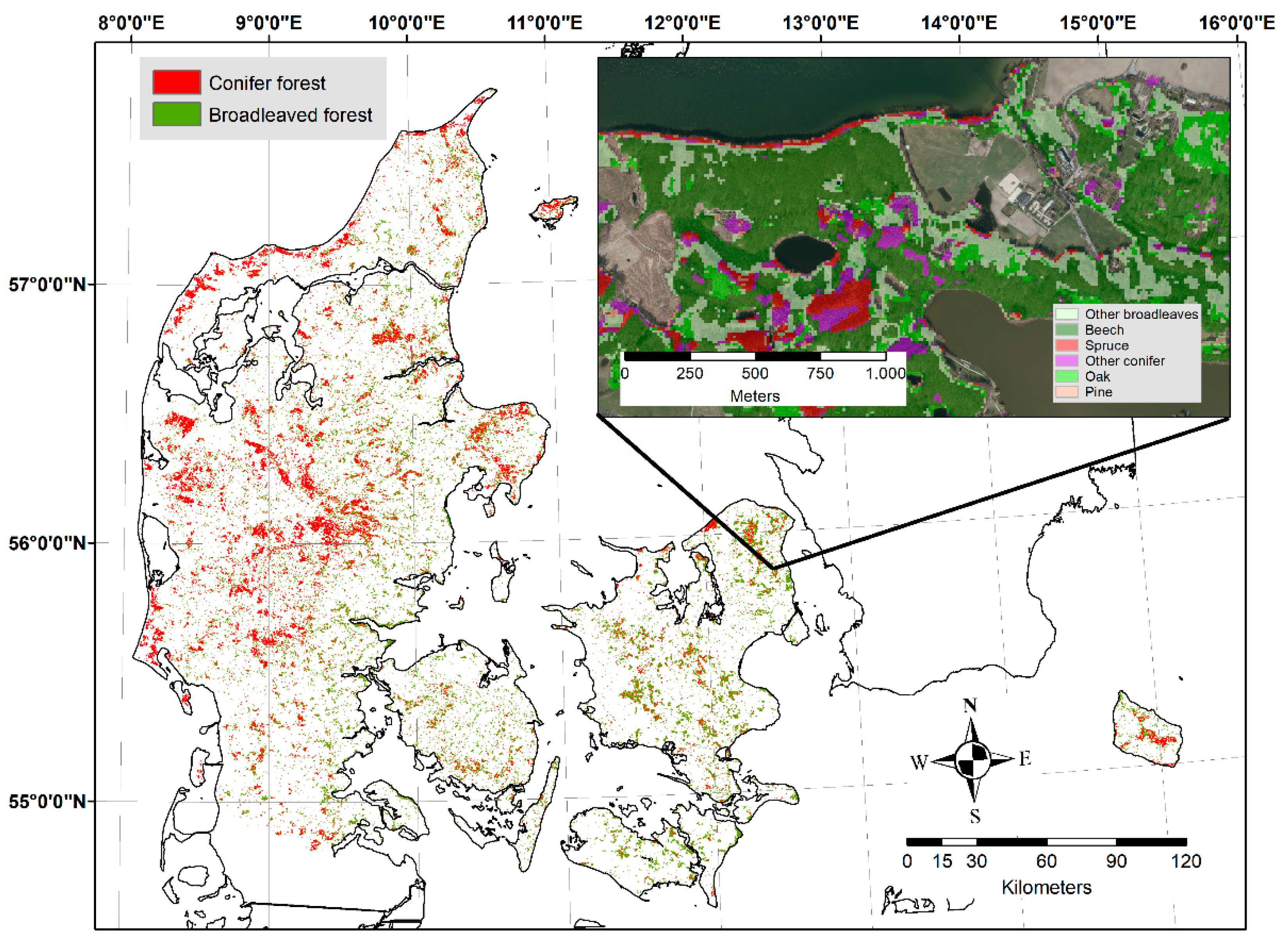
The resulting forest cover map of Denmark 2018 with details (see sections of forest type and species further below) from Frederiksdal Forest District, 17 km north of Copenhagen.
Figure 2.
The resulting forest cover map of Denmark 2018 with details (see sections of forest type and species further below) from Frederiksdal Forest District, 17 km north of Copenhagen.

Figure 3.
Input features for predicting forest type in Denmark 2018 ranked after importance by the Boruta simulations.
Figure 3.
Input features for predicting forest type in Denmark 2018 ranked after importance by the Boruta simulations.

Figure 4.
Input features for predicting tree species ranked after importance by the Boruta simulations.
Figure 4.
Input features for predicting tree species ranked after importance by the Boruta simulations.

Table 1.
Criteria for selecting reference NFI sample plots (SSUs) and number of training/evaluation plots for the different classification tasks, respectively. The fraction of ambiguous plots (i.e., plots that have a forest fraction <75% and/or a crown cover <10%) reflects the fragmented nature of Danish forests.
| Class | Criteria | Training (2018) | Evaluation (2017, 2019) |
|---|---|---|---|
| Forest cover | |||
| Non-forest | Forest fraction = 0% and crown cover = 0% | 6548 | 13,365 |
| Forest | Forest fraction > 75% and Crown cover > 10% | 981 | 1827 |
| Ambiguous | Not meeting above criteria | 965 | 1828 |
| Total | 8586 | 17,020 | |
| Forest type | Conifer/broadleaf species > 75% of basal area | ||
| Conifer | 319 | 532 | |
| Broadleaf | 357 | 650 | |
| Total | 676 | 1182 | |
| Tree species | Species group > 75% of basal area | ||
| Fagus | 75 | 165 | |
| Quercus | 57 | 93 | |
| Other broadleaves | 113 | 180 | |
| Picea | 99 | 203 | |
| Pinus | 74 | 125 | |
| Other conifers | 88 | 146 | |
| Total | 506 | 912 |
Table 2.
Confusion matrix and producer (PA), user (UA), and overall (OA) accuracy statistics for the raw forest cover classification (left) as well as for the post-filtered forest cover classification (right) based on the independent evaluation data. Entries in the matrix represent the number of pixels and proportions in brackets. Post filtering included the removal of forest areas smaller than the minimum mapping unit (0.5 ha) and forest in low build-up areas. The resulting forest areas and 95% confidence intervals (CI 95%) are based on the good practice for error-adjusted area estimation [63,64].
| Forest Cover | Reference | Reference (Post Filtered) | ||||
|---|---|---|---|---|---|---|
| Prediction | Non-Forest | Forest | Total | Non-Forest | Forest | Total |
| Non-forest | 13,236 (87.1%) | 174 (1.1%) | 13,410 | 13,325 (87.7%) | 191 (1.3%) | 13,516 |
| Forest | 129 (0.8%) | 1653 (10.9%) | 1782 | 40 (0.3%) | 1636 (10.8%) | 1676 |
| Total | 13,365 | 1827 | 15,192 | 13,365 | 1827 | 15,192 |
| PA | 0.99 | 0.90 | 1.00 | 0.90 | ||
| UA | 0.99 | 0.93 | 0.99 | 0.98 | ||
| OA | 0.98 | 0.98 | ||||
| Forest area (ha) | 637,290 | 597,980 | ||||
| CI 95% (ha) | ±10,402 | ±8573 | ||||
Table 3.
Confusion matrix and producer (PA), user (UA), and overall (OA) accuracy statistics of the forest type classification based on the independent evaluation data. Entries in the matrix represent the number of pixels and proportions in brackets. Forest area distribution to forest types and the corresponding 95% confidence interval (CI 95%) are based on the post-filtered forest area estimate (Table 2).
| Forest Type | Reference | ||
|---|---|---|---|
| Prediction | Conifer | Broadleaf | Total Pred. |
| Conifer | 503 (42.6%) | 27 (2.3%) | 530 |
| Broadleaf | 29 (2.5%) | 623 (52.7%) | 652 |
| Total ref. | 532 | 650 | 1182 |
| PA | 0.95 | 0.96 | |
| UA | 0.95 | 0.96 | |
| OA | 0.95 | ||
| Area (ha) | 268,824 | 329,156 | |
| CI 95% (ha) | ±7247 | ±7247 | |
Table 4.
Confusion matrix and producer (PA), user (UA), and overall (OA) accuracy statistics of the tree species classification based on the independent evaluation reference data. Entries in the matrix represent the number of pixels. Forest area distribution to forest tree species and the corresponding 95% confidence interval (CI 95%) are based on the post-filtered forest area estimate (Table 2).
| Reference | |||||||
|---|---|---|---|---|---|---|---|
| Prediction | Fagus | Quercus | Other Broadleaves | Picea | Pinus | Other Conifers | Total Pred. |
| Fagus | 104 | 17 | 35 | 2 | 0 | 6 | 164 |
| Quercus | 10 | 32 | 27 | 0 | 0 | 3 | 72 |
| Other broadleaves | 46 | 41 | 107 | 7 | 5 | 9 | 215 |
| Picea | 1 | 2 | 3 | 149 | 15 | 29 | 199 |
| Pinus | 1 | 0 | 4 | 11 | 92 | 4 | 112 |
| Other conifers | 3 | 1 | 4 | 34 | 13 | 95 | 150 |
| Total ref. | 165 | 93 | 180 | 203 | 125 | 146 | 912 |
| PA | 0.63 | 0.34 | 0.59 | 0.73 | 0.73 | 0.65 | |
| UA | 0.63 | 0.44 | 0.50 | 0.75 | 0.82 | 0.63 | |
| OA | 0.63 | ||||||
| Area (ha) | 112,759 | 66,089 | 133,160 | 119,273 | 70,271 | 96,428 | |
| CI 95% (ha) | ±13,423 | ±12,099 | ±15,209 | ±11,371 | ±8468 | ±11,761 | |
Publisher’s Note: MDPI stays neutral with regard to jurisdictional claims in published maps and institutional affiliations. |
© 2021 by the authors. Licensee MDPI, Basel, Switzerland. This article is an open access article distributed under the terms and conditions of the Creative Commons Attribution (CC BY) license (http://creativecommons.org/licenses/by/4.0/).
Share and Cite
MDPI and ACS Style
Bjerreskov, K.S.; Nord-Larsen, T.; Fensholt, R. Classification of Nemoral Forests with Fusion of Multi-Temporal Sentinel-1 and 2 Data. Remote Sens. 2021, 13, 950. https://0-doi-org.brum.beds.ac.uk/10.3390/rs13050950
AMA Style
Bjerreskov KS, Nord-Larsen T, Fensholt R. Classification of Nemoral Forests with Fusion of Multi-Temporal Sentinel-1 and 2 Data. Remote Sensing. 2021; 13(5):950. https://0-doi-org.brum.beds.ac.uk/10.3390/rs13050950
Chicago/Turabian StyleBjerreskov, Kristian Skau, Thomas Nord-Larsen, and Rasmus Fensholt. 2021. "Classification of Nemoral Forests with Fusion of Multi-Temporal Sentinel-1 and 2 Data" Remote Sensing 13, no. 5: 950. https://0-doi-org.brum.beds.ac.uk/10.3390/rs13050950
Note that from the first issue of 2016, this journal uses article numbers instead of page numbers. See further details here.