Article

A Two-Step Integrated MLP-GTWR Method to Estimate 1 km Land Surface Temperature with Complete Spatial Coverage in Humid, Cloudy Regions

1
State Key Laboratory of Urban and Regional Ecology, Research Center for Eco-Environmental Sciences, Chinese Academy of Sciences, Beijing 100085, China
2
Research Center for Eco-Environmental Sciences, Chinese Academy of Sciences, University of Chinese Academy of Sciences, Beijing 100049, China
3
Department of Earth and Planetary Sciences, Johns Hopkins University, 3400 North Charles Street, Baltimore, MD 21218, USA
*
Author to whom correspondence should be addressed.
Submission received: 14 January 2021 / Revised: 18 February 2021 / Accepted: 1 March 2021 / Published: 4 March 2021
(This article belongs to the Special Issue Land Surface Temperature Estimation Using Remote Sensing)

Abstract

:
There is an increasing demand for a land surface temperature (LST) dataset with both fine spatial and temporal resolutions due to the key role of LST in the Earth’s land–atmosphere system. Currently, the technique most commonly used to meet the demand is thermal infrared (TIR) remote sensing. However, cloud contamination interferes with TIR transmission through the atmosphere, limiting the potential of space-borne TIR sensors to provide the LST with complete spatio-temporal coverage. To solve this problem, we developed a two-step integrated method to: (i) estimate the 10-km LST with a high spatial coverage from passive microwave (PMW) data using the multilayer perceptron (MLP) model; and (ii) downscale the LST to 1 km and fill the gaps based on the geographically and temporally weighted regression (GTWR) model. Finally, the 1-km all-weather LST for cloudy pixels was fused with Aqua MODIS clear-sky LST via bias correction. This method was applied to produce the all-weather LST products for both daytime and nighttime during the years 2013–2018 in South China. The evaluations showed that the accuracy of the reproduced LST on cloudy days was comparable to that of the MODIS LST in terms of mean absolute error (2.29–2.65 K), root mean square error (2.92–3.25 K), and coefficients of determination (0.82–0.92) against the in situ measurements at four flux stations and ten automatic meteorological stations with various land cover types. The spatial and temporal analysis showed that the MLP-GTWR LST were highly consistent with the MODIS, in situ, and ERA5-Land LST, with the satisfactory ability to present the LST pattern under cloudy conditions. In addition, the MLP-GTWR method outperformed a gap-filling method and another TIR-PMW integrated method due to the local strategy in MLP and the consideration of temporal non-stationarity relationship in GTWR. Therefore, the test of the developed method in the frequently cloudy South China indicates the efficient potential for further application to other humid regions to generate the LST under cloudy condition.

1. Introduction

Land surface temperature (LST) plays an important role in the land surface energy balance, which influences the meteorological, hydrological, and biophysical processes in the land–atmosphere system of Earth [1,2,3,4,5]. LST data with high spatio-temporal resolution have found valuable application in land surface process models and the monitoring of soil moisture dynamics [6], frozen and burned areas [7,8], crop growth [9], and flash drought [10]. Therefore, LST estimation has been spotlighted by the Earth-observing community in recent years [11].
The development of satellite-based remote sensing (RS) techniques facilitates the long-term LST observations with high accuracy at regional and global scales, and thus the satellite-derived LST has been more widely used in practice than other sources (e.g., ground stations) [12]. One of the most widely used products is the LST dataset derived from the Moderate Resolution Imaging Spectroradiometer (MODIS), since it has high spatial resolution at nearly 1 km, a temporal interval of four times per day, global coverage, a twenty year long duration, and are easily and freely accessible [13]. Unfortunately, there are many large gaps in MODIS or other thermal infrared (TIR) -based LST images, limiting their utilities in related fields at their expected temporal scales [14,15]. This shortcoming is mainly caused by cloud interference, as the TIR sensors cannot penetrate thick cloud layers [16].
Many studies have attempted to recover the missing data in TIR-based LST products by developing a range of reconstruction approaches, which can be grouped into four types. The first type (I) is the gap-filling method. It relies on the spatial and temporal information of the clear neighboring LST pixels or other LST data from different satellites on the same day to create seamless LST datasets by substitution or interpolation [13,17,18,19,20]. These methods are usually not regionally specific and can be applied effectively at global scale. However, the gap-filled LST only represents the pattern under clear-sky conditions, without considering information under cloud cover. Moreover, multistep convolutions and iterations are required to fill large gaps in the gap-filling method, causing considerable accumulative error [13].
The second type of method (II) is based on the surface energy balance (SEB) equation to derive the cloudy-sky LST [12,20,21,22,23]. Generally, its performance depends primarily on the quality of input shortwave radiation (SW) and other complex regional parameterization (e.g., air temperature). Another disadvantage is that the SEB method is not able to be applied at nighttime when spatial variations in LST are not dominated by the SW input.
The third group (III) uses the outputted all-weather LST from the regional climate model (RCM) or land surface model (LSM) blended with the MODIS LST via data fusion approaches [24,25]. The outputs from RCM or LSM generally contain larger systematic bias and deviation compared to ground-based or RS-based observations and further bias correction is needed [25,26]. In addition, the computing demand of RCM or LSM increases exponentially with a finer scale and larger areas, impeding their usability in a fine scale in practice [27].
The fourth type of approach (IV) estimates the missing LST by building an empirical or physical relationship between the LST and its related auxiliary predictors [14,28,29,30,31,32]. Choosing suitable predictors that can indicate the sky condition is the key to achieving the accurate cloudy-sky LST retrieval. One of the widely used variables is the passive microwave (PMW) brightness temperature (BT). Since microwaves transmit through clouds and other sources of atmospheric interference, PMW sensors can provide the LST information under cloudy-sky condition [33]. Among the microwave bands, the Ka band (~37 GHz) is the most commonly used to estimate LST in previous studies [30,32,33,34,35]. Other bands (e.g., K band [28,29,36], X and C band [37]) are also incorporated to obtain the PMW LST.
However, there are some obstacles to integrating TIR and PMW observations to generate all-weather LST products. One clear problem is that PMW-based measurements typically have much coarser spatial resolution (i.e., 0.1°–0.25°) than the TIR-based LST (i.e., <~1 km). In some studies, interpolation is applied to resample the PMW-based BTs directly to match the TIR’s resolution [30,32]. Considering the spatial heterogeneity of LST, some studies have derived the PMW-based LST at the original coarse resolution and then downscaled it to the high resolution rather than resampling [14,28]. Yoo et al. (2020) reported the latter scheme had better performance for cloudy-sky daytime during the day [14]. Meanwhile, Peng et al. (2019) found that a downscaling strategy that considered both the spatial and temporal variabilities of LST outperformed algorithms that neglected the temporal information [38].
A second challenge for PMW-based LST estimation methods is the choice of a scheme between physically based or empirical algorithms [28,32,33]. Compared to physics-based retrieval algorithms, empirical models established between multi-channel PMW BTs and TIR clear-sky LST to estimate the cloudy-sky LST have shown satisfactory accuracy and high efficiency [14,39]. These models include applications of multiple linear regression (MLR) [30], artificial neural networks (ANN) [32], and random forests (RF) [14,39]. However, it remains unclear whether the design of the regression model (e.g., the global or local strategy) in these studies is applicable over multiple geographical environments in terms of the performance stability and computational complexity.
A third challenge to PMW-TIR fusion is that most PMW satellite sensors suffer from non-overlapping swaths, resulting in swath gaps between two adjacent orbits [39]. An extra gap-filling step, which is similar to the type (I) gap-filling method described above, is used to fill up the swath gap in the TIR-PMW integrated product to generate all-weather gap-free high-resolution LST [28,30]. Another feasible method is to generate the gap-free PMW BTs before integrating of the PMW and TIR LST [39].
This study introduces an improved two-step approach (MLP-GTWR) combining the multi-layer perceptron (MLP) with the moving window strategy and the geographically and temporally weighted regression (GTWR) model to better address the issues in TIR-PMW integration methods. We generated the all-weather LST maps with the same spatio-temporal resolution as the MODIS LST (MYD11A1) products over South China for the years 2013–2018, based on multiple remote sensing datasets. The feasibility of the generated all-weather LST for different land cover types were examined with comparisons against the in situ LST observations at four ground flux towers and ten automatic meteorological stations.

2. Study Area and Dataset

2.1. Study Area

The TIR-based RS technique for retrieving LST is particularly limited in humid regions due to the frequent cloud. Therefore, we chose South China as the study area, which mostly belongs to tropical and subtropical humid monsoon regions, with five Köppen–Geiger climate types (‘Am’, ‘Aw’, ‘Cwa’, ‘Cwb’, and ‘Cfa’; large lakes are masked) [40], and is mostly covered by forests and cropland (Figure 1a). This region has a distinct seasonal climate with hot and wet summers and cold and dry winters. In the hottest months (i.e., July and August), the average air temperature can reach 30 °C in the east interior and gradually decrease to 20 °C with increasing elevation in the west. The average air temperature in the coldest months (i.e., January) is mainly dominated by latitude, with 0 °C average temperatures found in the north and 15 °C in the south. Most precipitation occurs during the summer. The coverage of the MODIS LST is quite limited, with mostly less than 40% (Figure 1b). During summer, there are often several continuous weeks without much valid LST in MODIS products over a large region. Therefore, it is of high priority to reconstruct the cloudy-sky LST for South China for many LST applications.

2.2. Satellite-Based Datasets

2.2.1. Moderate Resolution Imaging Spectroradiometer (MODIS) Land Surface Temperature (LST) Data

The TIR LST data used in this study were 1-km MODIS Aqua LST products (MYD11A1, collection 6) with 1 km resolution, which are freely available from the Land Processes Distributed Active Archive Center (LP DAAC). These are derived from two TIR bands, 31 (10.78-11.28 μm) and 32 (11.77-12.27 μm), using the generalized split-window algorithm [41]. Pixels with the MODIS LST filtered by the quality flag (average LST error <=3 K and average emissivity error <=0.04) were identified as the valid clear-sky LST and others were the missing LST under cloudy conditions. This flag allows for much more available MODIS LST for training than the high-quality flag (error <=1 K) over our study area. The 1-km MODIS LST were aggregated to 10-km resolution by data averaging if there were more than 95% valid 1-km pixels in a 10-km AMSR2 grid cell.

2.2.2. Advanced Microwave Scanning Radiometer (AMSR2) Brightness Temperature Data

AMSR2 (Advanced Microwave Scanning Radiometer) is a dual polarized passive microwave radiometer and also the sister successor to AMSR-E. It was launched on the GCOM-W1 satellite in the orbit following Aqua in May 2012 and has observations from July 2012 up to now. The AMSR2 has a close observation time with the Aqua MODIS, allowing the integration of their PMW and TIR derived datasets [28]. It measures BTs at seven different channels (i.e., 6.9, 7.3, 10.7, 18.7, 23.8, 36.5, and 89.0 GHz in both horizontal (H) and vertical (V) polarization), with the spatial resolution varying from approximately 46.6 km at 6.9 GHz to 3.9 km at 89 GHz. This study used the level-3 daily 10-km gridded BTs of the AMSR2 BT data, which are provided by the Japan Aerospace Exploration Agency (JAXA) [42]. AMSR2 BTs at the 7.3, 23.8, and 89 GHz channels were not used in the study because the first was close to 6.9 GHz and the latter two are easily influenced by atmospheric effects [30].

2.2.3. Land Surface Feature Data

The land surface feature data used in this study include the 90-m digital elevation model (DEM) product of Shuttle Radar Topography Mission (SRTM), the 1-km and 10-day leaf area index (LAI), and fraction of vegetation cover (FVC) from version 2 of the COPERNICUS products [42], and the 500-m annual nighttime lights (NL) products of the Visible Infrared Imaging Radiometer Suite Day/Night Band (VIIRS-DNB) [43]. LAI and FVC are closely associated with LST variability due to plant surface properties and evapotranspiration [44], while the NL observations are highly related to the urban artificial surface ratio, which has a large impact on the local LST. All datasets were aggregated to 1-km and 10-km to match up to the MODIS and the AMSR2 spatial grids, respectively. The 10-day LAI and FVC products were also linearly interpolated to daily-scale. The NL were set to 0 or 65 when they were <1 or >65, respectively, to exclude the extremely high values and low background noise [45].

2.3. In Situ Measurements

We collected the surface upward and downward longwave radiation data from four sites of the ChinaFLUX Network [46] (Table 1, Figure 1a) to evaluate the generated all-weather LST. Three sites (Qianyanzhou, Dinghushan, and Xishuangbanna) are mainly covered by forests and the remaining one (Taoyuan) is cropland. High-resolution satellite imagery of the surrounding areas at four stations from Google Earth (Appendix A Figure A1) was used to judge the spatial homogeneity around the station at 1-km and 10-km scales. In addition, based on all available 30-m Landsat 8 clear-sky LST images (see details in Appendix A Table A1) in 2014 [47], the thermal heterogeneity (determined by the mean standard deviation (STD) of all sub-pixel LST within a MODIS pixel) at the four listed stations in Table 1 were calculated, and were found to be 0.84 K, 0.45 K, 0.45 K, and 1.06 K, respectively. These results demonstrate that the in situ LST measurement offers reasonable spatial representation to evaluate the 1-km pixel-scale LST for validation [48].
First, we removed the abnormal measurements with the quality check. The abnormal values were the upward or downward longwave radiation for which the difference was out of three times the standard deviations from their half-hour averaged observation series [49]. Then, the LST with the closest observation time to MODIS was calculated using the following Stefan–Boltzmann law for the validation:
T s = F ( 1 ε b ) F σ ε b 0.25
where Ts is the calculated LST; σ is the Stefan–Boltzmann constant; F and F are upward and downward longwave radiation from in situ measurements, respectively; and εb is surface broadband emissivity and can be estimated from narrowband emissivity [50]:
  ε b = 0.2122 ε 29 + 0.3859 ε 31 + 0.4029 ε 32
where ε29, ε31, and ε32 are the surface narrowband emissivity of MODIS bands 29, 31, and 32, respectively, derived from the MYD11C1 (day/night algorithm).
In order to evaluate the all-weather LST retrievals for more widespread land cover types and spatial coverages, the ground measured 0-cm LST at a total of ten automatic meteorological stations (AMS, see the spatial location in Figure 1b) from 2013 to 2018 from the China Meteorological Administration was also selected as reference data. To qualify for the LST homogeneity validation, these selected stations were required to have low thermal heterogeneity in LST (less than 1 K). The hourly in situ LST (1 a.m./p.m. and 2 a.m./p.m.) were linearly interpolated to match the MODIS view time. The various land cover types (e.g., urban and savannas) at the ten AMS sites can provide better representation to the study region than the four flux stations. However, the spatial scale differences between the pixel-based LST and the point-based AMS observations can lead to systematic bias. To solve this problem, a bias-correction method using polynomial regression [14] was applied to bias-correct the AMS in situ LST before it was used in validation.

2.4. Other Validation Data

The ERA5-Land 0.1° hourly dataset (Copernicus Climate Change Service) was used to evaluate the spatial performance of the generated all-weather LST. ERA5-Land is a replay of the land component of the ERA5 climate reanalysis, but has an enhanced spatial resolution (0.1°, ~9km). The instantaneous land surface temperatures were obtained from Copernicus Climate Change Service (C3S) and linearly interpolated in time to match the MODIS view time.

3. Methods

The multilayer perceptron-geographically and temporally weighted regression (MLP-GTWR) method is composed of three processes (Figure 2). The first process is to predict the 10-km daily all-weather LST by the MLP models; the second process is to downscale the 10-km LST to 1 km and fill the gaps with the GTWR method; and then the 1-km PMW-based gap-free all-weather LST is fused with the MODIS LST via bias correction. The following subsections illustrate the methods and validations in detail.

3.1. Multilayer Perceptron (MLP) Process with Moving Windows to Generate 10-km All-Weather Land Surface Temperature

Similar to the methodology presented in Jiménez et al. (2017) [34], we used the MLP model to establish the non-linear relationships between descriptors and the LST at the 10-km scale:
L S T v = M L P ( B T s , L A I , F V C , D E M ) + ε
where LSTv denotes the MODIS LST at the training stage and the LST prediction at the predicting stage; BTs represents the AMSR2 BTs of the four channels (6.9, 10.7, 18.7, and 36.5 GHz at both H and V polarization); ancillary data including the LAI, FVC, and DEM are involved to enhance the robustness of prediction; and M L P is the nonlinear function learned by the MLP model.
Although the application of one MLP model at global scale in Jiménez’s study showed good performance, we adapted it to a local scale by using a moving window strategy in this study for two reasons. First, a local strategy can more effectively characterize statistical relationships between LST and predictors over highly heterogeneous regions. Second, the representativeness of the training data (i.e., the TIR-based LST) to the overall data (i.e., the all-weather LST) distribution is often weak over a large region due to the differences in cloud frequency (Figure 1b). Thus, adopting local MLP models ensures better representativeness of training data, enabling better model performance. In this study, the window began from the northwestern corner of the region and moved in the direction from north to south and from west to east until it finally covered the entire region. The shape of the window was designed to be square (the upper left side of Figure 2). The length of the window was set to 90 km with a 10-km moving distance, showing the best performance in trial and error (Appendix A Figure A2c). The implemented moving window strategy consisted of four steps:
(1)
Set a square window and create the training data with all available MODIS LST in this window.
(2)
Train an MLP model used only in this window.
(3)
Predict the 10-km LST map using the trained MLP model.
(4)
Slide the window with a distance in the direction of right or down, and repeat steps 1–4 until covering the entire study area.
In the above steps, the moving windows are partially overlapping and a MLP model is trained/run using the pixels in each window. Therefore, the LST value of a pixel would have multiple candidates predicted from all MLP models with their windows including the pixel. The final value is obtained by averaging predictions with the outliers excluded (the difference between outliers and the mean is more than three times the standard deviation of all predictions):
p t ( L S T | ( T B s , L A I , F V C , D E M ) ) = 1 m i = 1 m p i ( L S T | ( B T s , L A I , F V C , D E M ) )
where pt is the final estimate of the missing LST; pi is one of the predictions from multiple MLP models; and m is the number of all accepted outputs. Using Equation (4), the predictions are much more stable and avoid extreme values.
The left side of Figure 2 illustrates the architecture of a MLP network with two hidden layers used in this study. It is composed of the input, two hidden, and output layers, which play the role of inputting predictor variables, solving nonlinear regression fittings, and generating predictions, respectively. Some settings including a rectified linear unit (ReLU) activation function, an adaptive moment estimation (Adam) gradient descent optimizer, and a mean squared error (MSE) loss function are used in training the MLP model. The collected training datasets (MODIS LST BTs, LAI, FVC, DEM) were divided into training (70%), validation (15%), and test (15%) sets randomly, and the final weight coefficients were assigned by the backpropagation (BP) algorithm to achieve the minimum MSE. To balance the performance of the MLP method and the consuming time of training, a grid search method [51] was applied to tune the structure of MLP models and two global parameters (Appendix A Figure A2). The optimal nodes in the first and second layers were 14 and 7. The loss function of each MLP network could easily reach its minimum error before 1000 iterations. The total number of MLP network was 21,760 and all of them could be trained and run in parallel. The MLP process was run in a MATLAB R2018b environment and completed in less than two days for the whole period of 2013–2018 on a computer with a dual-Xeon 24 core CPU.

3.2. Geographically and Temporally Weighted Regression (GTWR) Process to Downscale Land Surface Temperature

Based on the MLP models, daily 10-km LST maps (termed as the MLP LST) under both clear-sky and cloudy conditions were produced. However, the MLP LST does not have full coverage because there are missing BTs data due to the data gaps in AMSR2. To produce the 1-km LST with complete spatial coverage, the GTWR was implemented as a space–time model. This type of model has high predictive power since it uses both spatial and temporal information at a local scale [38,52,53]. In this study, we applied the GTWR model to quantify the association between the LST and four land surface features (DEM, LAI, FVC, and NL). The structure of the GTWR model is expressed as follows:
L S T i = β 0 ( u i , v i , t i ) + β 1 ( u i , v i , t i ) × D E M i + β 2 ( u i , v i , t i ) × L A I i + β 3 ( u i , v i , t i ) × F V C i + β 4 ( u i , v i , t i ) × N L i + ε i
where (ui,vi,ti) denotes the space–time location of a pixel i; β0(ui,vi,ti) is the intercept and β1–β4 are the local coefficients estimated at the pixel i for DEM, LAI, FVC, and NL, respectively; LSTi is the land surface temperature of the pixel i; and εi is the regression residual.
To estimate the β(ui,vi,ti) parameters in the GTWR model, we used the ‘optimization method’ proposed by Huang et al. (2010) [53], which applies the Gaussian distance decay-based functions and the combination of spatial and temporal distance to calculate the weight matrix W. The W accounts for the importance of sample j to sample i in spatial and temporal scale. It is weighted by two parameters: the spatio-temporal bandwidth hST, reflecting a decay of importance with distance, and the scale factor ρ, reflecting the relative influence between space and time. To decrease the computing time of the GTWR process, we fixed hST to 90 km·day, which is the size of the moving window in the MLP process, and selected the optimal value of ρ through the leave-one-out cross-validation method [53,54,55].
After establishing the nonstationary regression relationship between the LST and the four land surface features on the 10-km scale, the parameters (i.e., the intercept and local coefficients β(ui,vi,ti)) were interpolated to 1 km using the ordinary kriging interpolation. The isotropic spherical semi-variogram model was selected, which best fit the relationship between the distance and the experimental semivariogram values. As the kriging interpolation technique was used to downscale and the 10-km pixels were evenly distributed in space, we only used one sector and fixed the maximum neighbors to 20 in the search neighborhood. These parameters satisfied the conditions below: (1) The prediction error (RMSE) was close to the smallest value in cross validation; (2) The kriging weights were mostly positive and larger than 0.01; and (3) The computational cost was acceptable. Based on the assumption that the relationship between variables is much more scale-invariant than the data itself, the 1-km daily all-weather LST (termed as MLP-GTWR LST) for the years 2013–2018 were generated using the four 1-km features as the inputs of the downscaled regression relationship. The GTWR model, meanwhile, can capture the spatial and temporal pattern of the LST space and time series at local scale (Equation (5)), which makes it possible to reconstruct the complete 1-km LST map series without the swath gaps.

3.3. Bias Correction

To make the MLP-GTWR LST closer to the MODIS LST, we used the linear and variance scaling approaches [56,57] to bias-correct the MLP-GTWR LST. The part of the MODIS 1-km LST that was excluded in the aggregation to 10 km and not involved in the MLP-GTWR process was used as the correction target. The systematic biases between the MODIS LST and the MLP-GTWR LST was minimized with equations:
B ias = μ ( L S T M L P G T W R , c l e a r ) μ ( L S T M O D I S , c l e a r )
L S T M L P G T W R bias c o r r e c t e d = L S T M L P G T W R B i a s
L S T M L P G T W R zero m e a n = L S T M L P G T W R b i a s c o r r e c t e d μ ( L S T M L P G T W R b i a s c o r r e c t e d )
L S T M L P G T W R , c o r = μ ( L S T M L P G T W R bias - corrected ) + L S T M L P G T W R z e r o m e a n σ ( L S T M O D I S , c l e a r ) σ ( L S T M L P G T W R , c l e a r z e r o m e a n )
where LSTMLP-GTWR,cor is the MLP-GTWR LST with corrected bias and deviation; μ and σ denote the mean and standard deviation of the corresponding data, respectively; and the subscript ‘clear’ means the part of the data under clear-sky condition.
Through the linear and variance scaling process, it was assumed that the bias and standard deviation for clear-sky pixels remained unvaried for cloudy pixels. Thus, the bias-corrected MLP-GTWR LST (termed as the MLP-GTWR LSTcor) had no systematic bias and deviation with the MODIS LST and its cloudy part can be fused with the MODIS LST to generate the final 1-km gap-free all-weather LST products.

3.4. Evaluation

To evaluate the performance of the MLP-GTWR model, several statistical metrics were used: the bias, mean absolute error (MAE), root mean square error (RMSE), and the coefficient of determination (R2). The MLP-GTWR LST before bias correction was inter-compared with MODIS LST (for pixels not involved in the MLP-GTWR process) to assess the performance of the method for clear pixels. Then, the bias-corrected MLP-GTWR LST was evaluated against in situ measurements at the four flux towers and ten AMS sites under both clear-sky and cloudy-sky conditions to assess the performance of all three stages of the proposed method. The spatial and temporal maps of the MLP-GTWR LSTcor are presented to evaluate consistency with other LST estimates (i.e., the MODIS, in situ, and ERA5-Land). In addition, the MLP-GTWR method is compared with a gap-filling method [19] and another PMW-TIR integrated method [32].

4. Results

4.1. Performance Evaluation of the MLP-GTWR Method Evaluated with MODIS LST

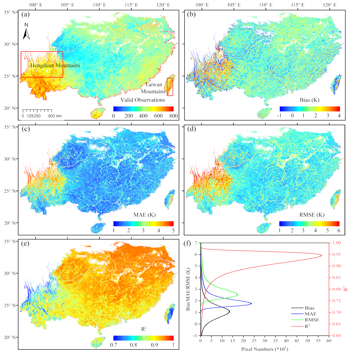
Figure 3 shows the comparison between the MLP-GTWR LST (not bias-corrected) and the 1-km MODIS LST for clear pixels across the entire study area. After the MLP and GTWR processes, the overall mean bias, MAE, RMSE, and R2 between both LSTs were 1.17 K, 2.15 K, 2.99 K, and 0.91, respectively, and the standard deviations of the bias, MAE, RMSE, and R2 were 0.87 K, 0.72 K, 0.85K, and 0.05, respectively. The result that the RMSE was less than 3 K and the R2 was higher than 0.9 in most regions indicates a close agreement between the MLP-GTWR LST and MODIS LST under clear-sky conditions.
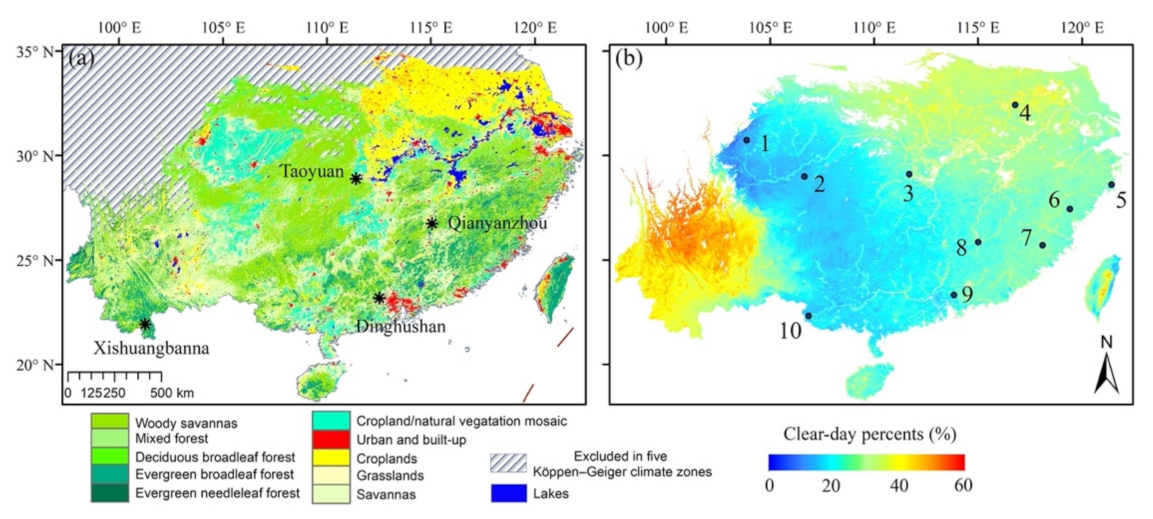
The spatial patterns of the four metrics showed that the performance varied in space in a manner that was not highly related to the clear-day percentage of MODIS LST and the land cover type (Figure 1 and Figure 3). Although satisfactory performance and high correlation existed in most of South China, three regions could be recognized with relatively higher error: the Southwestern Hengduan Mountains, Taiwan Mountains, and the areas near river channels or lakes. Some studies have reported that the strong topographic effects on radiative environment would induce large retrieval bias in PMW BTs over high-mountain regions [58,59]. Additionally, the largest uncertainty in the MODIS LST retrieval (i.e., MYD11A1) was calculated using fixed surface emissivity determined by the land cover type [48]. However, in mountainous regions, the snow and the plant cover are quite dynamic and can have strong seasonality, leading to high uncertainty in estimates of surface emissivity as well as LST.
For land surfaces with a high proportion of water areas (e.g., lakes and flooded soil), the LST retrieval based on the PMW BTs was expected to exhibit weaker performance due to lower BTs and higher polarization differences for water [60]. Therefore, there would be large discrepancies between the AMSR2 and MODIS observations over those three regions, resulting in lower accuracy of the generated MLP-GTWR LST compared to other areas. Therefore, it was necessary to correct the systematic biases of the MLP-GTWR LST using the bias correction method before merging with the MODIS LST.

4.2. Performance Evaluation of the MLP-GTWR Method Evaluated with In Situ Measurements
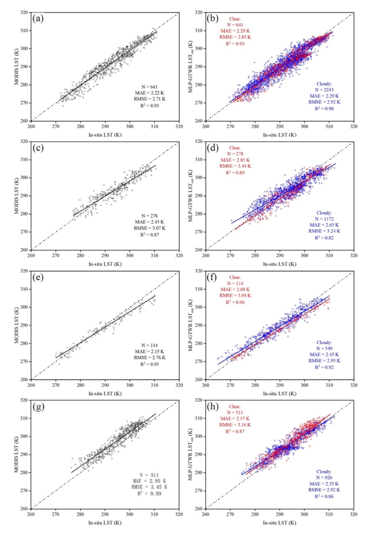
The scatterplots in Figure 4 show the comparison of the MLP-GTWR LSTcor and MODIS LST against the in situ LST measurements at four flux towers. The former all-weather LST was divided into two parts: clear-sky and cloudy-sky, decided by the MODIS clear-sky LST. Overall, the measured in situ LST showed good agreement with the MODIS LST at four sites, with MAE, RMSE, and R2 varying between 2.15–2.95 K, 2.72–3.45 K, and 0.88–0.95, respectively. The metrics of the flux-based in situ LST used in this study were comparable to those from the literature involving the validation of the MODIS LST [25,48], indicating a good spatial representative to evaluate the 1-km gridded LST. For the MLP-GTWR LSTcor under clear-sky conditions, the MAE, RMSE, and R2 varied within the range of 2.29–2.85 K, 2.83–3.44 K, and 0.87–0.96, respectively. These results certify that the performance of the MLP-GTWR LSTcor under clear-sky condition is comparable and similar to that of the MODIS LST at all flux sites.
For the cloudy-sky groups of the MLP-GTWR LSTcor, the MAE, RMSE, and R2 ranged from 2.29 K to 2.65 K, from 2.92 K to 3.24 K, and from 0.82 to 0.92, respectively. Overall, the performance of the all-weather MLP-GTWR LSTcor was generally similar between the clear-sky and cloudy-sky conditions versus the in situ measurements at four flux towers. The RMSE of the MLP-GTWR LSTcor under cloudy-sky condition was slightly lower than that under clear-sky condition at the Dinghushan, Taoyuan, and Xishuangbanna flux stations. This can be attributed to the lower thermal spatial heterogeneity under cloudy-sky conditions on account of lower shortwave radiation. This decreases uncertainty arising from the scale-mismatch between the flux-based observation and a 1-km pixel in validation.
In addition, separate validations of the MLP-GTWR LSTcor for daytime and nighttime on clear and cloudy days would offer a better understanding of the performance of the MLP-GTWR method (Table 2). The statistical metrics for daytime and nighttime are both similar to those shown in Figure 4, supporting the above results that the difference of the accuracy was not significant between the MLP-GTWR LSTcor and the MODIS LST during the day as well as at night.
In addition to this broad area evaluation, the MLP-GTWR LSTcor was compared with the bias-corrected 0-cm temperature at ten AMS sites. Statistics are listed in Table 3. The performance of the MLP-GTWR LSTcor under cloudy-sky condition was worse than that under clear-sky conditions based on the AMS temperature, which was different from the results from three flux stations. It is worth noting that the measurement was sampled at a single point for the AMS instruments, which may fluctuate more than a spatially averaged flux tower footprint or a satellite retrieval if rain, snow, or strong wind is present under cloudy conditions. This effect may exaggerate the scale-mismatch issue between the AMS observations and 1-km LST, causing higher uncertainty in the validation.
Among the AMS sites, seven had RMSE difference between the clear-sky and cloudy-sky condition lower than 0.5 K, while one site covered by the savannas and both urban sites had larger RMSE differences of 0.68 K, 0.66 K, and 1.09 K, respectively. The likely reason is that microwave radiometry usually faces a radio frequency interference (RFI) problem over urban areas, inducing large uncertainty on AMSR2 BTs as well as the MLP-GTWR LSTcor [61]. Combining evaluations against in situ measurements at the four flux towers and ten AMS sites, the result revealed that the proposed MLP-GTWR method could generate all-weather LST estimates reasonably well.
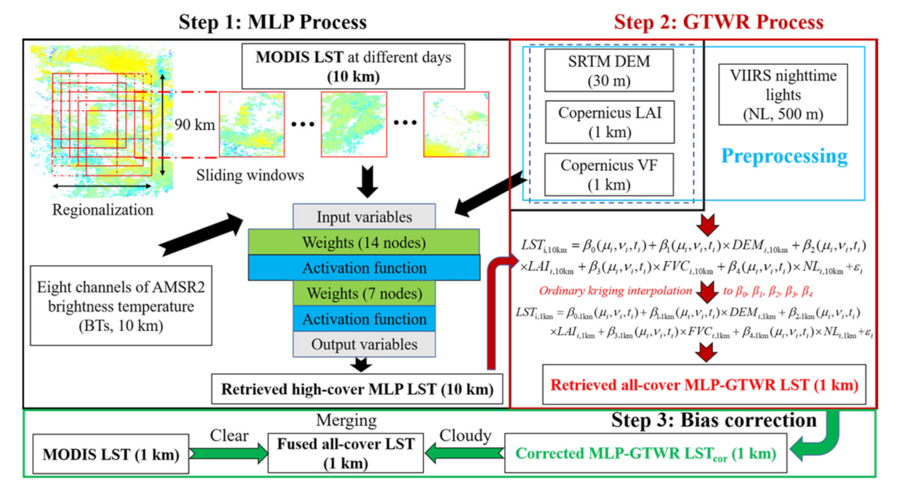
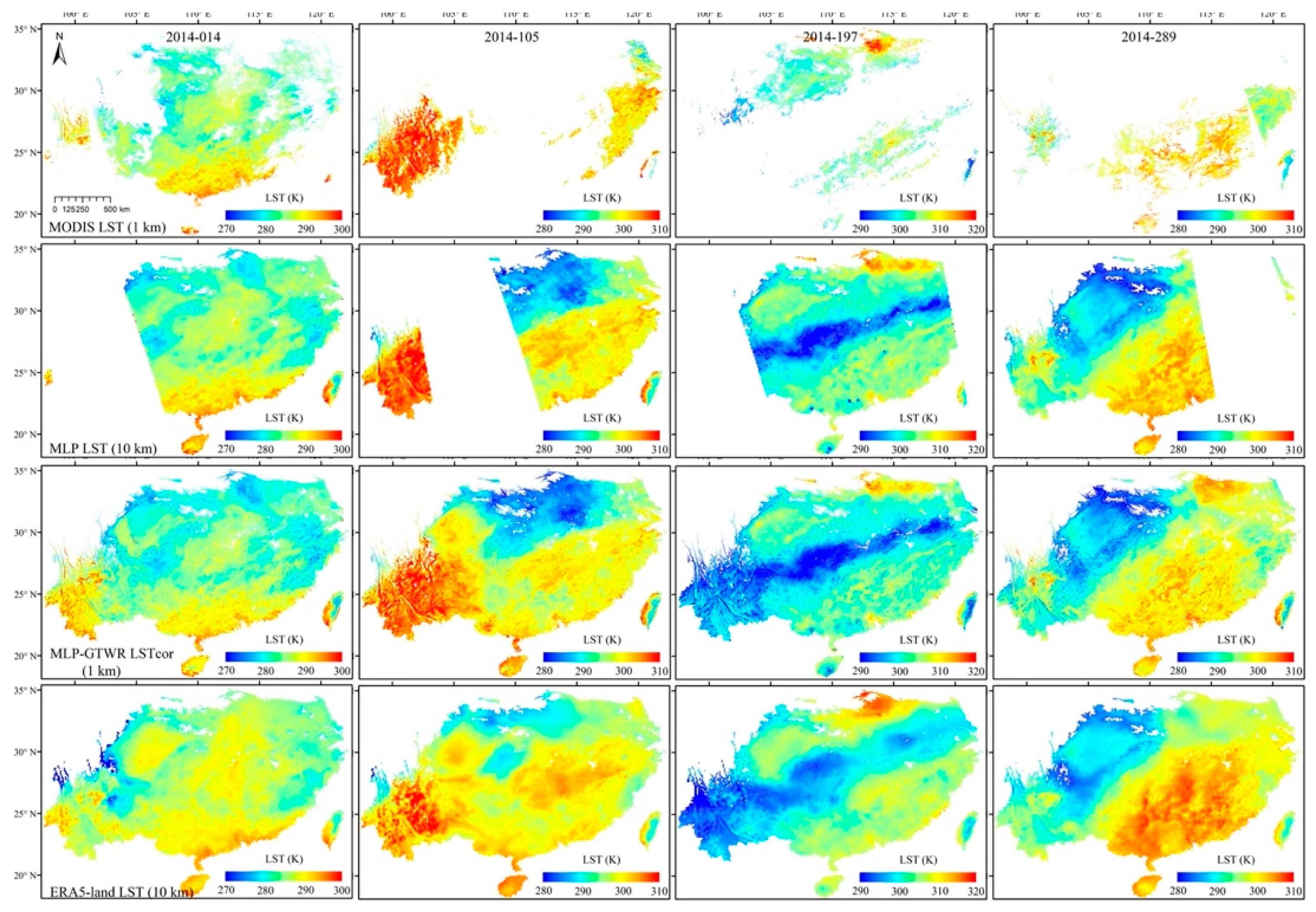
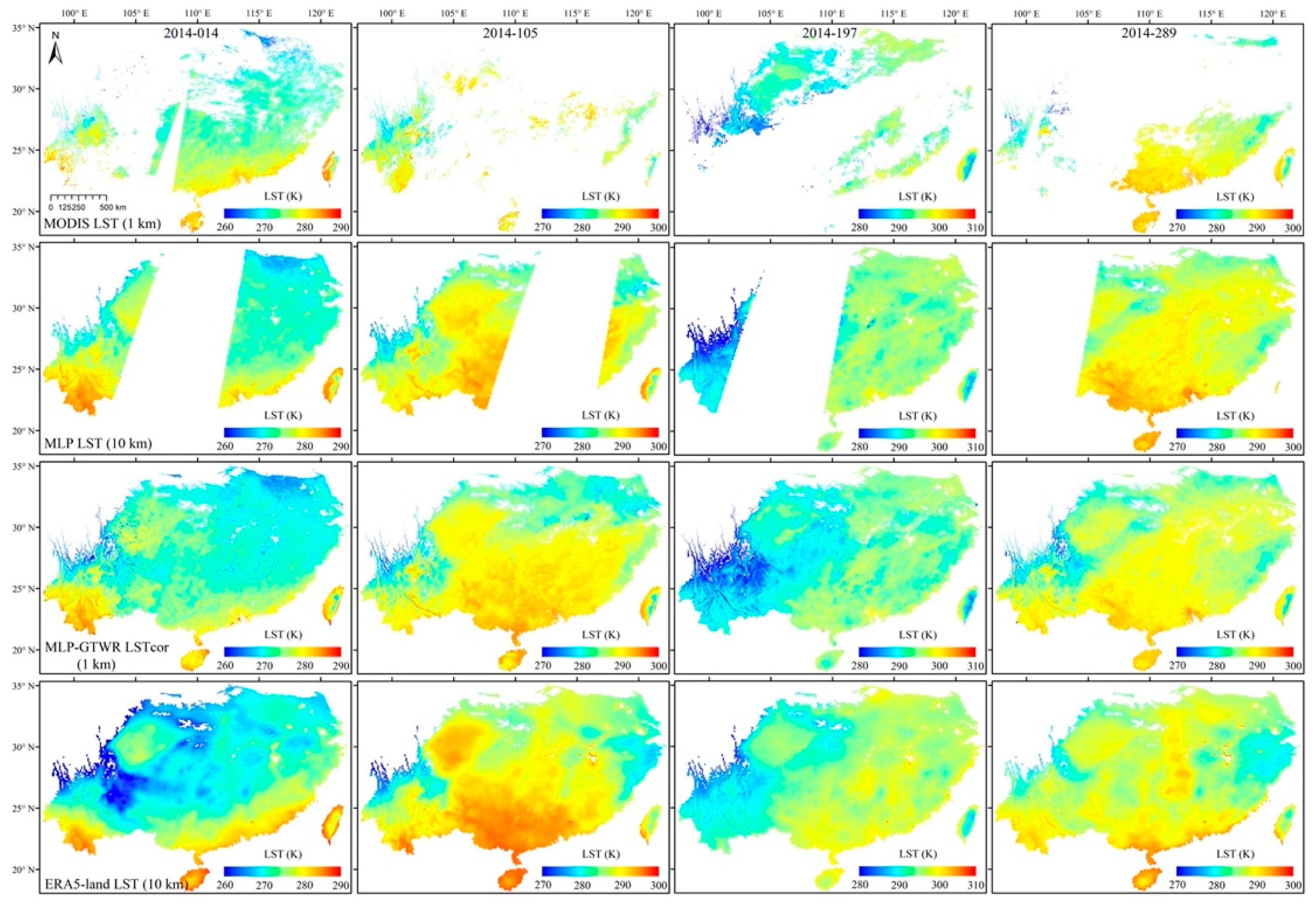
As our proposed method is composed of two major processes (i.e., MLP and GTWR) and one correction step, it produces three LST products with two spatial resolutions: the 10-km MLP LST, 1-km MLP-GTWR LST, and bias-corrected MLP-GTWR LSTcor, sequentially. These LST products were compared against the in situ LST measurements to illustrate the change of errors in different steps (Figure 5). Note that only the in situ LST from four flux towers was used as a comparison object to ensure the better reliability. From the 10-km MODIS LST to the 10-km MLP LST in the MLP process, the MAE, RMSE, and R2 changed from the range of 1.98–2.41 K, 2.43–2.92 K, and 0.90–0.96 to 2.20–2.38 K, 2.77–3.02 K, and 0.88–0.94. Considering the in situ LST may not be suitable for the 10-km LST comparison due to the large spatial scale difference, the 0.1° ERA5-Land LST product was also used as a reference (Table 4). The results against the ERA5-Land LST also showed a similar change in the MAE, RMSE, and R2 from 1.64–3.49 K, 2.11–4.00 K, and 0.88–0.96 to 1.61–3.80 K, 2.14–4.54 K, and 0.84–0.94. It is evident that the MLP LST had a larger error than the MODIS LST. However, considering that the former is under all-weather condition, the increased error is still at an acceptable level with the MLP process.
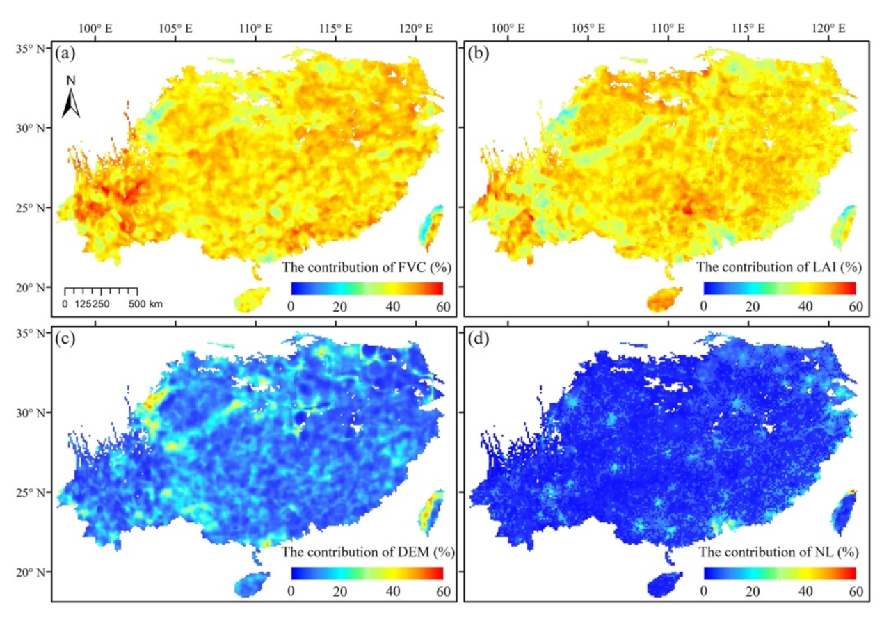
The GTWR process downscaled the 10-km MLP LST to the 1-km MLP-GTWR LST and filled the swath gaps. The comparison showed that this process made non-significant changes in the errors at the Qianyanzhou and Taoyuan sites, while the Dinghushan and Xishuangbanna sites had an increased error, according to the MAE, RMSE, and R2 (Figure 5). Using Dinghushan as an example, the MAE increased from 2.21 K to 2.53 K, the RMSE increased from 2.92 K to 3.10 K, and the R2 decreased from 0.88 to 0.83. Dinghushan and Xishuangbanna are both located at tropical areas and covered with rainforest, which have low variations of FVC and LAI in a year. This may be the reason why the GTWR model performed worse on predicting the fine-scale LST. Overall, the introduced error in the GTWR process was considerably small, indicating the satisfactory performance of the GTWR method in downscaling and gap-filling.
In the bias correction, the MLP-GTWR LST was corrected to the MODIS LST rather than to the in situ data, resulting in the bias of the MLP-GTWR LSTcor closer to that of the MODIS LST (Figure 5). There was nonsignificant improvement within bias correction at the Qianyanzhou, Dinghushan, and Taoyuan sites, perhaps due to the low bias and deviation between the clear-sky LST in Equations (7) and (9) (Figure 3). However, the bias correction aimed to improve the agreement between the MLP-GTWR and MODIS LST over some regions with large discrepancies (see Section 4.1 and Figure 3), especially the Hengduan and Taiwan mountains. It is very challenging to evaluate our approach over these regions due to the lack of suitable in situ measurements with good representativeness to the gridded LST. Moreover, the appliance of the bias correction made it more reasonable to further merge the MLP-GTWR LSTcor and MODIS LST to generate the best 1-km all-weather LST.

4.3. Spatial Variability in the MLP-GTWR LSTcor

To evaluate the spatial variability of the produced LST, the 1-km MODIS LST, 10-km MLP LST, and 1-km MLP-GTWR LSTcor are shown for four days in 2014 (i.e., 14th, 105th, 197th, and 289th), which were the mid-days of four seasons (Figure 6 and Figure 7). The ERA5-Land LST is also displayed to provide the all-weather LST pattern from a LSM. The large irregular gaps existed in the MODIS LST because of the cloud contamination. In contrast, the 10-km MLP LST filled up the missing data except the regular AMSR2 swath gaps. Compared to the MODIS and MLP LST, the MLP-GTWR LSTcor not only had high consistency in matters of the spatial and temporal variations, but also provided the complete spatial details of LST information. A similar consistency was also found from comparison between the MLP-GTWR LSTcor and ERA5-Land product over the cloudy areas. For instance, the daytime LST on the 197th day in the central area was obviously lower than the surrounding area due to heavy precipitation events (Appendix A Figure A3). The MLP-GTWR LSTcor captured this LST pattern correctly with the ERA5-Land. In addition, the MLP-GTWR LSTcor images showed wonderful spatial continuity and ignorable block effects even at the edges of the swath gaps. These results demonstrate the satisfactory efficiency of the GTWR method as the second step in downscaling and gap-filling the coarse-resolution LST to fine-resolution images.

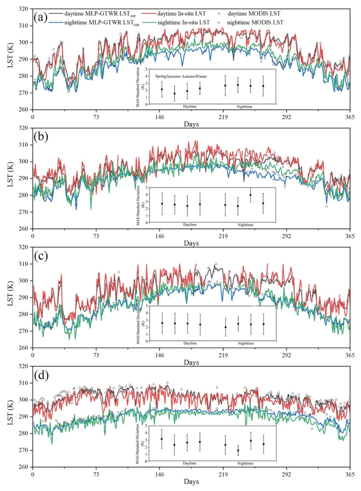
4.4. Temporal Variability in the MLP-GTWR LSTcor

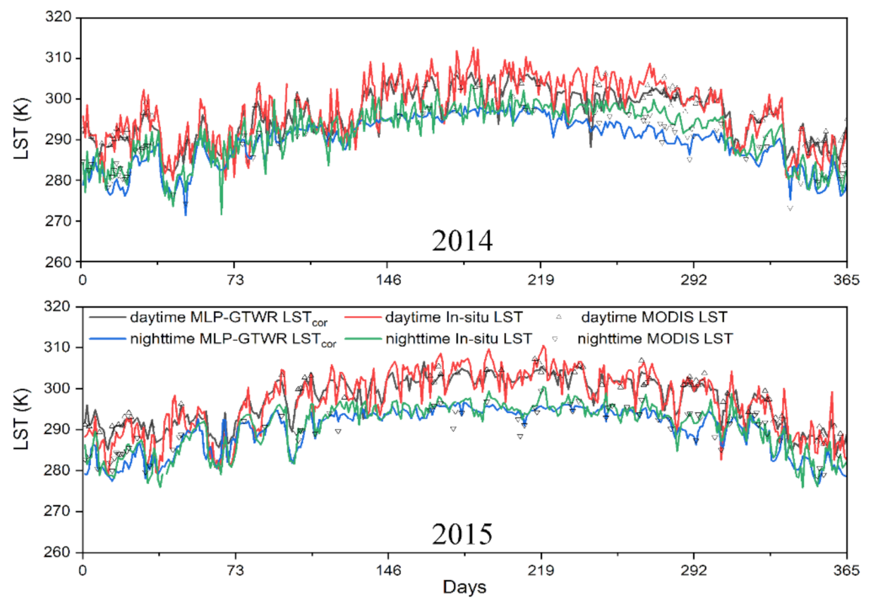
As the observation periods at the four flux stations all included the year 2014, the time series of the MLP-GTWR LSTcor and in situ measurements are shown in 2014 (
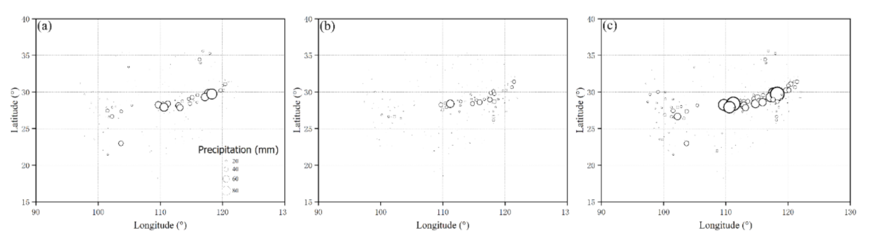
Figure 8). One can see that the MLP-GTWR LSTcor had high similarity in the temporal variation with the in situ measurements and MODIS LST in both daytime and nighttime at different stations. In most cases, the MLP-GTWR LSTcor could capture a sudden LST change following the in situ LST when the MODIS LST was missing, associated with precipitation events. However, when some extreme situations occur, particularly within a single day (e.g., a short-term precipitation occurs and the AMSR2 data are missing), the LST image could exhibit a different pattern with neighboring pixels in space and time. This means that there was not enough information to retrieve the missing LST without introducing more uncertainty. Using the LST or radiation output from an LSM may be an alternative to the MLP LST to achieve better LST retrievals over orbit gaps in these cases.
Furthermore, the performance of the MLP-GTWR LSTcor at daytime and nighttime varied among sites (subplots in Figure 8). For example, the MAE was lower for daytime than nighttime at Qianyanzhou, but the opposite result occurred at Xishuangbanna. In terms of the standard deviations, no evident difference was shown for the accuracy between different seasons in most cases. The performance of the MLP-GTWR LSTcor in summer can be comparable and even better than other seasons, although the MODIS LST had the fewest valid observations during summer. This indicates that the performance of the MLP-GTWR method is less impacted by the uneven temporal distribution of the MODIS LST. Some large biases between the MLP-GTWR LSTcor exist in some sites and in some seasons, for example, in the summer at Qianyanzhou, in the autumn at Dinghushan, or in the autumn/winter at Xishuangbanna in 2014. However, using the clear-sky MODIS LST (the target in this study) as the reference, our modeled LST had smaller bias than the ground LST in most cases. When comparing the remote sensing-based LST with in situ measurements, the monthly/season mean bias between them was variable among sites and time (Duan et al., 2019). In addition, obvious bias was shown between the MLP-GTWR LSTcor and in situ measurements during the 230th to 310th day in the year 2014, but a similar phenomenon was not found in 2015 (Appendix A Figure A4). Overall, the analysis of the spatio-temporal variability of the all-weather MLP-GTWR LSTcor confirms the great stability and reliability of the MLP-GTWR approach over South China.

5. Discussion

5.1. The Advantages of the MLP and GTWR Processes in the Proposed Two-Step Method

The proposed MLP-GTWR method has two main steps, the MLP and GTWR, achieving the retrieval of the coarse-resolution LST and downscaling it to 1 km as well as gap-filling, respectively. The MLP model was chosen in this study rather than other well-documented models (e.g., MLR and RF) [14,30] for two reasons. First, as a type of artificial neural network (ANN), the MLP model is capable of mapping the complex relationship between the LST and PMW BTs better than MLR. Second, the moving window strategy was applied to ensure the representativeness of the training data and improve the performance over heterogenous areas, thus a large number of regression models were trained. The computational cost of the MLP model is relatively low compared to other machine learning algorithms (e.g., RF and deep learning), as it has few hidden layers and nodes. Meanwhile, the method comparison in Dong et al. (2020) suggests that the MLP model can achieve better forecasting efficiency than MLR and RF when using only low-dimension predictor variables [62]. Therefore, the MLP model is pretty ideal for this study to take over the LST prediction considering the trade-off between the robustness and the computation cost.
Theoretically, the GTWR model has the ability to generate the 1-km missing LST without the MLP process (Equation (5)), but some disadvantages limit its practical application for that purpose. Since the MODIS valid LST are usually distributed irregularly in space and time, the GTWR model needs to search the optimal parameter values (i.e., hST and ρ) for each pixel (ui,vi,ti) to elucidate the quantitative association β(ui,vi,ti). The parameter selection involves the usage of a nested-loop, thus consuming large computation time. Moreover, when large gaps exist in the training data, the prediction power of the GTWR method is much weakened. However, to a large extent, using the MLP LST as the training data, instead of the MODIS LST, addresses these shortcomings. The MLP LST is spread much more evenly in space and time (Figure 6 and Figure 7, the second row), allowing a general fixed bandwidth in our study. Our results showed that the performance of the GTWR model using a bandwidth of 90 km·day was robust across South China with the computation cost decreasing dramatically.
To investigate the superiority of the GTWR method in downscaling the LST to the MLP model itself or other regression models (e.g., RF), the MLP model was retrained and rerun with the bilinearly interpolated 1-km AMSR BTs to simulate the 1-km all-weather LST directly (one-step scheme) for 2014. The comparison results between the one-step MLP scheme and two-step MLP-GTWR method against the in situ measurements at four flux towers are listed in Table 5. The two-step method had a better performance than the one-step scheme at the Qianyanzhou, Taoyuan, and Xishuangbanna stations, while the performance was similar at the Dinghushan station. The land cover was relatively homogeneous (Appendix A Figure A1) and the spatial thermal heterogeneity was very low (0.45 K) at Dinghushan, which may explain the similar accuracy between these two methods.
The two-step MLP-GTWR method performed better than the one-step method for at least two reasons. First, the GTWR method can explicitly capture both the spatial and temporal variations in the local-scale relationship [52] from the time series dataset of the LST, the FVC, and the LAI, while other algorithms usually neglect the temporal variations. Peng et al. (2019) demonstrated that the temporal information in the GTWR-based algorithm also helped weaken the smoothing effect and remove the blocking effect [38]. Second, the relationship between LST and other auxiliary variables is more scale-invariant than the data itself, and thus interpolation to the data directly should be avoided. In a word, the proposed two-step MLP-GTWR method combines the advantages and addresses the disadvantages of the two individual methods to improve the performance of all-weather LST products.

5.2. The Relative Importance of the Predictors in the MLP-GTWR Method

To analyze the importance of each variable to the LST predicting accuracy in the MLP process, the permutation importance test was performed by retraining the MLP model with 50 replications independently, where one of the variables is randomly shuffled while others remain constant [63]. The relative importance of a variable is presented by the ratio of the increased RMSE to the sum for all variables (Figure 9). The AMSR2 BTs play the most crucial role (the all contribution >80%) in retrieving the missing 10-km LST. The 36.5 vertical (V) and horizonal (H) channels were identified as the two most important predictors (with a contribution of 25.9% and 14.4%, respectively). Previous studies have commonly used the 36.5 GHz (Ka-band) BT to estimate the LST [30,33], since it has low sensitivity to soil surface parameters and atmospheric effects. Due to the ability to distinguish the land surface’s vegetation cover and soil moisture conditions [37], the 6.9(V) and 18.7(V) channels also had relatively high contributions of 12.9% and 12.5%, respectively. The lower frequencies in the 6.9 and 10.7 GHz channels allowed for observations neglecting the atmospheric effect. However, the coarser spatial resolution and the greater sampling depth of these channels introduced potential errors in describing the pattern of vegetation and veg/soil moisture, thus contributing less in LST retrieval. The land surface features including DEM, FVC, and LAI were also helpful in improving the retrieval accuracy with a total contribution of 10.6%. Overall, the vertical polarization channels were more important than the corresponding horizontal polarization channels. This can be explained by the lower dielectric constant for water and lower sensitivity to changes in soil moisture with the vertically polarized channels [60]. Besides, all variables played a positive role in improving the accuracy of the LST retrievals in the MLP process.
The Pratt index [64], which is the multiplication of the standardized regression coefficient and the Pearson correlation coefficient r between the LST and each variable, was used to assess each feature’s importance in the GTWR model. The four features had different contributions in downscaling the LST across South China, obviously varied in space (Figure 10). The FVC and LAI, which are important indexes to describe the surface vegetation conditions, explain most of the spatio-temporal variance in LST downscaling. This result indicates the validity of the FVC and LAI as the scaling factors in the GTWR model over the study region. The regions with lower significant contribution of the FVC and LAI were the transition zone between high mountains/plateau and flat plain/basin (e.g., the northwest edge of the study region, western Taiwan) and urbanized areas (e.g., the delta of Yangtze/Pearl River, northern Taiwan). The DEM is the main factor dominating the spatial pattern of LST in the former areas, while the strong impact of urban build-up and artificial surface on the LST make a significant contribution over urban areas, which can be identified by the nighttime lights.

5.3. Comparison of the MLP-GTWR Method with a Gap-Filling Method and a Same-Type Method

To evaluate our method, we applied a gap filling method [19] and a same-type PMW-TIR-based integrated method [32] to reconstruct the LST for comparison. Both methods are classic approaches that have been widely used in type (I) and (IV) LST reconstruction methods. For example, Li et al. (2018) used only the MOD/MYD clear-sky LST to reconstruct the hypothetical LST on cloudy-sky days with daily merging and spatio-temporal gap-filling methods. Shwetha and Kumar (2016), in contrast, trained separate ANN models for each land cover class, employing the geolocation information and Julian day as extra inputs. Using the above two methods, we estimated the corresponding 1-km LST under cloudy-sky conditions over the areas (61 km × 61 km) surrounding the four flux towers for the year 2014.
Figure 11 shows the scatterplots of the comparison of the MLP-GTWR LSTcor and the above two reconstructed LST against the in situ measurements at the four flux towers. The metrics at each station are presented in Appendix A Table A2 and Appendix A Table A3 in detail. The results showed a better performance of the MLP-GTWR method than Li’s gap-filling method in terms of the overall MAE (2.49 vs. 3.68 K), RMSE (3.05 vs. 4.85), and R2 (0.89 vs. 0.73). One challenge for the method used by Li et al. (2018) is that the larger the domain of missing values in the MODIS images, the more spatio-temporal gap-filling iterations are required. Since our study area has high-frequency cloud coverage, the uncertainty and accumulative errors were considerable in Li’s gap-filling method. In contrast, by integrating AMSR2 BTs, the MLP-GTWR method resulted in more stable LST estimation over cloudy regions.
The MLP-GTWR method also outperformed Shwetha’s one-step scheme in our study region. Where the Shwetha’s one-step approach uses geolocation and time as predictor variables directly, the MLP-GTWR method exploits this information in two ways. First, the MLP model is locally trained over a moving window region, allowing for improved data representation and better characterization of local relationships. Second, the GTWR model optimizes the synergy of spatial and temporal dimensions in the data to enhance the overall performance and present detailed LST distributions. In addition to the methodological advantages described in Section 5.1 (e.g., two-step vs. one-step method), incorporating multi-channel bands of AMSR2 BTs and a vegetation index into the predictors notably improved performance for this study region (Section 5.2).

5.4. Limitations and Potential for Further Applications

In this study, we used the 10-km AMSR2 BTs to reconstruct the cloudy-sky LST over South China and obtained the all-weather LST with similar accuracy to the MODIS LST. One important reason was the close agreement between the PMW and TIR -derived LST observations over the humid areas with dense vegetation and high surface soil moisture [33,34,65]. The penetration depth of the PMW measurements was small for a wet top-soil layer (e.g., ~1 mm at 37 GHz), close to the depth TIR-derived LST refers to (~50 μm). Over dense vegetated areas, both the PMW and TIR -derived LST are for the canopy layer (Holmes et al., 2009). However, the PMW sampling depth would be larger over arid regions, causing larger uncertainty to the all-weather LST. In addition, previous studies have used single, two, or multi- PMW bands in LST retrieval [14,28,29,30,33,66]. In terms of our study, eight channels in the AMSR2 were applied to guarantee the generalization of LST estimation for the entire South China. For instance, the low-frequency bands (i.e., 6.9 and 10.7 GHz) can provide more information about surface radiation for paddy fields and wetlands, as these bands are less absorbed and scattered by water, but have lower contributions and would increase the model complexity in other land cover types. The value of different combinations of PMW bands for estimating LST over various land cover types warrants further study. Therefore, the impact of the AMSR2 BTs on the performance of the MLP-GTWR model needs to be examined for more regions with different climate and land cover types (especially over the desert).
In addition, the MLP models established under clear-sky conditions were applied to generate the cloudy-sky LST in this study. Considering that the atmospheric conditions and thermal processes are different under clear-sky and cloudy-sky conditions, it may lead to potential systematic bias in the cloudy-sky LST estimation. The result in this study indicates that the assumption that the fitted model under clear-sky conditions could perform well under cloudy conditions with satisfactory accuracy, which agreed with the conclusion in other studies [14,32,39,67]. In the future, with the development of the radiation variables (e.g., incident solar radiation) with fine spatio-temporal resolution, they can be good indicators of the cloud coverage to achieve the better guess of the cloudy-sky LST. Furthermore, the parameters of the ‘moving window’ technique (e.g., the shape and the size of the window, the moving distance of adjacent windows) need to be fully explored to achieve optimal applications in other regions.
The predictor variables and scaling factors chosen in this study (i.e., FVC, LAI, DEM, and NL) are highly related to the LST variations and show effective abilities in retrieving the cloudy-sky LST in this study. As the study region of South China is under a humid climate and has a high percentage of vegetation, we acknowledge that these scaling factors may not be suitable for other different regions such as arid and cold land. To facilitate the global implementation, some additional land surface parameters (e.g., albedo, terrain slope/aspect, snow index, or building index) should be further investigated to improve the reliability of the MLP-GTWR method in other regions. Additionally, the level-3 product of MODIS LST and AMSR2 BTs were applied to generate the all-weather LST datasets since the former two products are extensively used in practical applications. To further improve the accuracy of the final all-weather LST, the level-2 swath datasets should be applied to match up the observation time by removing the data with large time difference or applying temporal calibration to achieve better matching.

6. Conclusions

In this study, we proposed a two-step MLP-GTWR method to generate the all-weather LST based on the MODIS LST, AMSR2 BTs, and four land surface features. This method was applied to retrieval the all-weather LST datasets at both daytime and nighttime across South China, for the years 2013–2018. When validated against in situ measurements from four flux stations, the bias-corrected MLP-GTWR LST had a MAE of 2.29–2.85 K, RMSE of 2.83–3.44 K, and R2 of 0.87–0.96 under the clear-sky conditions, and a MAE of 2.29–2.65 K, RMSE of 2.92–3.24 K, and R2 of 0.82–0.92 under cloudy-sky conditions. Similar results were also concluded when compared to the 0-cm temperature at ten automatic meteorological stations, validating the robustness of the method. The spatial and temporal variability of the MLP-GTWR LSTcor showed high consistency with the MODIS LST, in situ measurements, and ERA5-Land LST, and can present the LST pattern correctly under cloudy conditions. In addition, the MLP-GTWR method outperformed a gap-filling method and a same-type PMW-based method due to the local strategy in the MLP model and the consideration of the spatio-temporal non-stationarity of the relationship between LST and four factors in the GTWR model. Overall, the proposed scheme incorporating four LST-related ancillary variables could generate the all-weather LST with satisfactory quality in South China. The MLP-GTWR method is completely based on satellite remote sensing products and can be easily implemented. Therefore, our method can help produce high spatio-temporal LST images with complete spatial coverage and facilitate research on finer scales in other similar humid areas severely impacted by frequent clouds.

Author Contributions

Conceptualization, Z.G. and Y.H.; Methodology and validation, Z.G. and Y.C.; Writing—original draft preparation: Z.G.; Writing—review and editing, Z.G., Y.H., B.F.Z., and W.C.; Funding acquisition, Y.H. and W.C. All authors have read and agreed to the published version of the manuscript.

Funding

The work is supported by the National Key R&D Program of China (2019YFB2102902 and 2017YFC0505702) and the Chinese Academy of Sciences (QYZDB-SSW-DQC034). Zhen Gao is supported by China Scholarship Council (No. 201904910497).

Institutional Review Board Statement

Not applicable.

Informed Consent Statement

Not applicable.

Data Availability Statement

Publicly available datasets were used in this study. These data can be found here: https://lpdaac.usgs.gov/products/myd11a1v006/ (accessed on 1 March 2021), https://suzaku.eorc.jaxa.jp/GCOM_W (accessed on 6 October), https://www.ngdc.noaa.gov/eog/ (accessed on 1 March 2021), https://cds.climate.copernicus.eu (accessed on 1 March 2021), www.chinaflux.org (accessed on 2 March 2021), http://data.cma.cn/ (accessed on 3 March 2021). The final all-weather LST maps presented in this study in the year 2014 can be accessed from https://drive.google.com/file/d/13ErqW2JSZLZVde14DZ59QfBTR9FDSLHl/view?usp=sharing (accessed on 3 March 2021). The all-weather LST in other years are available upon reasonable request from the author Z.G.

Acknowledgments

We would like to thank Guirui Yu and Zhi Chen from the Institute of Geographic Sciences and Natural Resources Research (Chinese Academy of Sciences), the four ChinaFLUX stations, and CMA meteorological stations that shared the data used for validation in this project.

Conflicts of Interest

The authors declare no conflict of interest.

Appendix A

Figure A1. High-resolution satellite imagery (Google Earth) of the surrounding areas of the four flux stations listed in Tab. 1. The position of the stations is in the center and marked by the black-circle dots. (a,b) Qianyanzhou, (c,d) Dinghushan, (e,f) Taoyuan, and (g,h) Xishuangbanna. The left and right column is at the scale of 10 km and 1 km, respectively. The red rectangles in the left column mark the areas in the right column. The scale legend and north arrow is located at the bottom right corner.
Remotesensing 13 00971 g0a1
Figure A2. Sensitivity analysis of the node numbers of the two-layer multilayer perceptron model and the length of sliding window. (a) Performance change with the first hidden layer with the fixed node 10 in the second hidden layer. (b) Performance change with the second hidden layer with the fixed node 14 in the first hidden layer. (c) Performance change with the window length with the fixed sliding distance 10 km (one grid’s size). The RMSE is calculated from the comparison of the test sets (15% of the training dataset) and their corresponding predictions in the MLP model. Considering the computing time cost, the final nodes in two layers are chosen to be 14 and 7, and the window size is 90 in the MLP process.
Remotesensing 13 00971 g0a2
Figure A3. The precipitation recorded by the ground meteorological stations at the 197th day in 2014 across South China. (a) the total precipitation in the period of 20:00-08:00. (b) the total precipitation in the period of 08:00-20:00. (c) the total precipitation of both (a) and (b). The precipitation data is downloaded from China Meteorological Administration ().
Remotesensing 13 00971 g0a3
Figure A4. Temporal variations in daytime and nighttime MODIS LST, MLP-GTWR LSTcor, and in-situ measurements at Dinghushan station in the year 2014 (top) and 2015 (bottom).
Remotesensing 13 00971 g0a4
Table A1. The number of available Landsat 8 images used to calculate the thermal heterogeneity at four flux sites.
StationTotalSpringSummerAutumnWinter
Qianyanzhou142453
Dinghushan82231
Taoyuan72221
Xishuangbanna114133
Table A2. Comparison of the MLP-GTWR LSTcor and the fused LST from MODIS data using Li’s method [19] against the in-situ measurements at four flux towers. The statistical metrics at each site are shown.
MetricsQianyanzhouDinghushanTaoyuanXishuangbanna
MLP-GTWRLi’s ApproachMLP-GTWRLi’s ApproachMLP-GTWRLi’s ApproachMLP-GTWRLi’s Approach
Bias−0.42−0.85−1.99−1.83−0.94−0.542.162.16
MAE2.254.012.943.112.473.242.502.96
RMSE2.815.263.553.922.994.033.013.80
R20.910.750.870.820.950.850.940.84
Table A3. Comparison of the MLP-GTWR LSTcor and the downscaled LST using Shwetha’s method [32] against the in-situ measurements at four flux towers. The statistical metrics at each site are shown.
MetricsQianyanzhouDinghushanTaoyuanXishuangbanna
MLP-GTWRShwetha ’s ApproachMLP-GTWRShwetha ’s ApproachMLP-GTWRShwetha ’s ApproachMLP-GTWRShwetha ’s Approach
Bias−0.511.62−1.88−1.08−0.931.531.762.69
MAE2.354.332.903.562.413.472.253.33
RMSE2.955.683.514.332.914.642.814.42
R20.890.650.850.690.910.790.900.75

References

  1. Janatian, N.; Sadeghi, M.; Sanaeinejad, S.H.; Bakhshian, E.; Farid, A.; Hasheminia, S.M.; Ghazanfari, S. A statistical framework for estimating air temperature using MODIS land surface temperature data: Estimating air temperature using modis land surface temperature. Int. J. Climatol. 2017, 37, 1181–1194. [Google Scholar] [CrossRef]
  2. Silvestro, F.; Gabellani, S.; Delogu, F.; Rudari, R.; Boni, G. Exploiting remote sensing land surface temperature in distributed hydrological modelling: The example of the Continuum Model. Hydrol. Earth Syst. Sci. 2013, 17, 39–62. [Google Scholar] [CrossRef] [Green Version]
  3. Zhang, Y.; Liang, S. Impacts of land cover transitions on surface temperature in China based on satellite observations. Environ. Res. Lett. 2018, 13, 024010. [Google Scholar] [CrossRef]
  4. Tomlinson, C.J.; Chapman, L.; Thornes, J.E.; Baker, C. Remote sensing land surface temperature for meteorology and climatology: A review. Meteorol. Appl. 2011, 18, 296–306. [Google Scholar] [CrossRef] [Green Version]
  5. Srivastava, P.K.; Han, D.; Ramirez, M.R.; Islam, T. Machine learning techniques for downscaling SMOS satellite soil moisture using MODIS land surface temperature for hydrological application. Water Resour. Manag. 2013, 27, 3127–3144. [Google Scholar] [CrossRef]
  6. Colliander, A.; Fisher, J.B.; Halverson, G.; Merlin, O.; Misra, S.; Bindlish, R.; Jackson, T.J.; Yueh, S. Spatial downscaling of SMAP soil moisture using MODIS land surface temperature and NDVI during SMAPVEX15. IEEE Geosci. Remote Sens. Lett. 2017, 14, 2107–2111. [Google Scholar] [CrossRef]
  7. Hu, T.; Zhao, T.; Shi, J.; Wu, S.; Liu, D.; Qin, H.; Zhao, K. High-resolution mapping of freeze/thaw status in China via fusion of MODIS and AMSR2 data. Remote Sens. 2017, 9, 1339. [Google Scholar] [CrossRef] [Green Version]
  8. Quintano, C.; Fernandez-Manso, A.; Roberts, D.A. Burn severity mapping from landsat MESMA fraction images and land surface temperature. Remote Sens. Environ. 2017, 190, 83–95. [Google Scholar] [CrossRef]
  9. Khanal, S.; Fulton, J.; Shearer, S. An overview of current and potential applications of thermal remote sensing in precision agriculture. Comput. Electron. Agric. 2017, 139, 22–32. [Google Scholar] [CrossRef]
  10. Nguyen, H.; Wheeler, M.C.; Otkin, J.A.; Cowan, T.; Frost, A.; Stone, R. Using the evaporative stress index to monitor flash drought in Australia. Environ. Res. Lett. 2019, 14, 064016. [Google Scholar] [CrossRef] [Green Version]
  11. Phan, T.N.; Kappas, M. Application of MODIS land surface temperature data: A systematic literature review and analysis. J. Appl. Remote Sens. 2018, 12, 1. [Google Scholar] [CrossRef]
  12. Jin, M.; Dickinson, R.E. A generalized algorithm for retrieving cloudy sky skin temperature from satellite thermal infrared radiances. J. Geophys. Res. Atmospheres 2000, 105, 27037–27047. [Google Scholar] [CrossRef]
  13. Pede, T.; Mountrakis, G. An empirical comparison of interpolation methods for MODIS 8-day land surface temperature composites across the conterminous Unites States. ISPRS J. Photogramm. Remote Sens. 2018, 142, 137–150. [Google Scholar] [CrossRef]
  14. Yoo, C.; Im, J.; Cho, D.; Yokoya, N.; Xia, J.; Bechtel, B. Estimation of all-weather 1 Km MODIS land surface temperature for humid summer days. Remote Sens. 2020, 12, 1398. [Google Scholar] [CrossRef]
  15. Rao, Y.; Liang, S.; Wang, D.; Yu, Y.; Song, Z.; Zhou, Y.; Shen, M.; Xu, B. Estimating daily average surface air temperature using satellite land surface temperature and top-of-atmosphere radiation products over the tibetan plateau. Remote Sens. Environ. 2019, 234, 111462. [Google Scholar] [CrossRef]
  16. Li, Z.-L.; Tang, B.-H.; Wu, H.; Ren, H.; Yan, G.; Wan, Z.; Trigo, I.F.; Sobrino, J.A. Satellite-Derived Land Surface Temperature: Current Status and Perspectives. Remote Sens. Environ. 2013, 131, 14–37. [Google Scholar] [CrossRef] [Green Version]
  17. Ghafarian Malamiri, H.R.; Rousta, I.; Olafsson, H.; Zare, H.; Zhang, H. Gap-filling of MODIS time series land surface temperature (LST) products using singular spectrum analysis (SSA). Atmosphere 2018, 9, 334. [Google Scholar] [CrossRef] [Green Version]
  18. Kang, J.; Tan, J.; Jin, R.; Li, X.; Zhang, Y. Reconstruction of MODIS land surface temperature products based on multi-temporal information. Remote Sens. 2018, 10, 1112. [Google Scholar] [CrossRef] [Green Version]
  19. Li, X.; Zhou, Y.; Asrar, G.R.; Zhu, Z. Creating a seamless 1 Km resolution daily land surface temperature dataset for urban and surrounding areas in the conterminous United States. Remote Sens. Environ. 2018, 206, 84–97. [Google Scholar] [CrossRef]
  20. Yu, W.; Tan, J.; Ma, M.; Li, X.; She, X.; Song, Z. An effective similar-pixel reconstruction of the high-frequency cloud-covered areas of Southwest China. Remote Sens. 2019, 11, 336. [Google Scholar] [CrossRef] [Green Version]
  21. Wang, T.; Shi, J.; Ma, Y.; Husi, L.; Comyn-Platt, E.; Ji, D.; Zhao, T.; Xiong, C. Recovering land surface temperature under cloudy skies considering the solar-cloud-satellite geometry: Application to MODIS and landsat-8 data. J. Geophys. Res. Atmos. 2019, 124, 3401–3416. [Google Scholar] [CrossRef]
  22. Yang, Y.; Smith, J.; Yang, L.; Baeck, M.L.; Ni, G. Regional impacts of urban irrigation on surface heat fluxes and rainfall in Central Arizona. J. Geophys. Res. Atmos. 2019, 124, 6393–6410. [Google Scholar] [CrossRef]
  23. Zeng, C.; Long, D.; Shen, H.; Wu, P.; Cui, Y.; Hong, Y. A two-step framework for reconstructing remotely sensed land surface temperatures contaminated by cloud. ISPRS J. Photogramm. Remote Sens. 2018, 141, 30–45. [Google Scholar] [CrossRef]
  24. Fu, P.; Xie, Y.; Weng, Q.; Myint, S.; Meacham-Hensold, K.; Bernacchi, C. A Physical model-based method for retrieving urban land surface temperatures under cloudy conditions. Remote Sens. Environ. 2019, 230, 111191. [Google Scholar] [CrossRef]
  25. Long, D.; Yan, L.; Bai, L.; Zhang, C.; Li, X.; Lei, H.; Yang, H.; Tian, F.; Zeng, C.; Meng, X.; et al. Generation of MODIS-like land surface temperatures under all-weather conditions based on a data fusion approach. Remote Sens. Environ. 2020, 246, 111863. [Google Scholar] [CrossRef]
  26. Xia, H.; Chen, Y.; Li, Y.; Quan, J. Combining kernel-driven and fusion-based methods to generate daily high-spatial-resolution land surface temperatures. Remote Sens. Environ. 2019, 224, 259–274. [Google Scholar] [CrossRef]
  27. Rummukainen, M. State-of-the-art with regional climate models. WIREs Clim. Chang. 2010, 1, 82–96. [Google Scholar] [CrossRef]
  28. Duan, S.-B.; Li, Z.-L.; Leng, P. A Framework for the retrieval of all-weather land surface temperature at a high spatial resolution from polar-orbiting thermal infrared and passive microwave data. Remote Sens. Environ. 2017, 195, 107–117. [Google Scholar] [CrossRef]
  29. Huang, C.; Duan, S.-B.; Jiang, X.-G.; Han, X.-J.; Leng, P.; Gao, M.-F.; Li, Z.-L. A physically based algorithm for retrieving land surface temperature under cloudy conditions from AMSR2 passive microwave measurements. Int. J. Remote Sens. 2019, 40, 1828–1843. [Google Scholar] [CrossRef]
  30. Zhang, X.; Zhou, J.; Gottsche, F.-M.; Zhan, W.; Liu, S.; Cao, R. A Method based on temporal component decomposition for estimating 1-km all-weather land surface temperature by merging satellite thermal infrared and passive microwave observations. IEEE Trans. Geosci. Remote Sens. 2019, 57, 4670–4691. [Google Scholar] [CrossRef]
  31. Kou, X.; Jiang, L.; Bo, Y.; Yan, S.; Chai, L. Estimation of land surface temperature through blending MODIS and AMSR-E data with the bayesian maximum entropy method. Remote Sens. 2016, 8, 105. [Google Scholar] [CrossRef] [Green Version]
  32. Shwetha, H.R.; Kumar, D.N. Prediction of high spatio-temporal resolution land surface temperature under cloudy conditions using microwave vegetation index and ANN. ISPRS J. Photogramm. Remote Sens. 2016, 117, 40–55. [Google Scholar] [CrossRef]
  33. Holmes, T.R.H.; De Jeu, R.A.M.; Owe, M.; Dolman, A.J. Land surface temperature from Ka Band (37 GHz) passive microwave observations. J. Geophys. Res. 2009, 114, D04113. [Google Scholar] [CrossRef] [Green Version]
  34. Jiménez, C.; Prigent, C.; Ermida, S.L.; Moncet, J.-L. Inversion of AMSR-E observations for land surface temperature estimation: 1. methodology and evaluation with station temperature. J. Geophys. Res. Atmos. 2017, 122, 3330–3347. [Google Scholar] [CrossRef]
  35. Owe, M.; Griend, A.A.V.D. On the relationship between thermodynamic surface temperature and high-frequency (37 GHz) vertically polarized brightness temperature under semi-arid conditions. Int. J. Remote Sens. 2001, 22, 3521–3532. [Google Scholar] [CrossRef]
  36. Weng, F.; Grody, N.C. Physical retrieval of land surface temperature using the special sensor microwave imager. J. Geophys. Res. Atmos. 1998, 103, 8839–8848. [Google Scholar] [CrossRef]
  37. Chen, J.; Zhu, X.; Vogelmann, J.E.; Gao, F.; Jin, S. A simple and effective method for filling gaps in landsat ETM+ SLC-off images. Remote Sens. Environ. 2011, 115, 1053–1064. [Google Scholar] [CrossRef]
  38. Peng, Y.; Li, W.; Luo, X.; Li, H. A Geographically and temporally weighted regression model for spatial downscaling of MODIS land surface temperatures over urban heterogeneous regions. IEEE Trans. Geosci. Remote Sens. 2019, 57, 5012–5027. [Google Scholar] [CrossRef]
  39. Zhang, X.; Zhou, J.; Liang, S.; Chai, L.; Wang, D.; Liu, J. Estimation of 1-km all-weather remotely sensed land surface temperature based on reconstructed spatial-seamless satellite passive microwave brightness temperature and thermal infrared data. ISPRS J. Photogramm. Remote Sens. 2020, 167, 321–344. [Google Scholar] [CrossRef]
  40. Kottek, M.; Grieser, J.; Beck, C.; Rudolf, B.; Rubel, F. World map of the Köppen-Geiger climate classification updated. Meteorol. Z. 2006, 15, 259–263. [Google Scholar] [CrossRef]
  41. Wan, Z.; Dozier, J. A Generalized split-window algorithm for retrieving land-surface temperature from space. IEEE Trans. Geosci. Remote Sens. 1996, 34, 892–905. [Google Scholar] [CrossRef] [Green Version]
  42. Baret, F.; Weiss, M.; Lacaze, R.; Camacho, F.; Makhmara, H.; Pacholcyzk, P.; Smets, B. GEOV1: LAI and FAPAR essential climate variables and FCOVER global time series capitalizing over existing products. Part 1: Principles of development and production. Remote Sens. Environ. 2013, 137, 299–309. [Google Scholar] [CrossRef]
  43. Baugh, K.; Hsu, F.-C.; Elvidge, C.D.; Zhizhin, M. Nighttime lights compositing using the VIIRS day-night band: Preliminary results. Proc. Asia-Pac. Adv. Netw. 2013, 35, 70–86. [Google Scholar] [CrossRef] [Green Version]
  44. Duveiller, G.; Hooker, J.; Cescatti, A. The mark of vegetation change on earth’s surface energy balance. Nat. Commun. 2018, 9, 1–12. [Google Scholar] [CrossRef] [Green Version]
  45. Guo, W.; Lu, D.; Wu, Y.; Zhang, J. Mapping impervious surface distribution with integration of SNNP VIIRS-DNB and MODIS NDVI Data. Remote Sens. 2015, 7, 12459–12477. [Google Scholar] [CrossRef] [Green Version]
  46. Yu, G.-R.; Wen, X.-F.; Sun, X.-M.; Tanner, B.D.; Lee, X.; Chen, J.-Y. Overview of ChinaFLUX and evaluation of its eddy covariance measurement. Agric. For. Meteorol. 2006, 137, 125–137. [Google Scholar] [CrossRef]
  47. Ermida, S.L.; Soares, P.; Mantas, V.; Göttsche, F.-M.; Trigo, I.F. Google Earth Engine open-source code for land surface temperature estimation from the landsat series. Remote Sens. 2020, 12, 1471. [Google Scholar] [CrossRef]
  48. Duan, S.-B.; Li, Z.-L.; Li, H.; Göttsche, F.-M.; Wu, H.; Zhao, W.; Leng, P.; Zhang, X.; Coll, C. Validation of collection 6 MODIS land surface temperature product using in situ measurements. Remote Sens. Environ. 2019, 225, 16–29. [Google Scholar] [CrossRef] [Green Version]
  49. Göttsche, F.-M.; Olesen, F.-S.; Trigo, I.F.; Bork-Unkelbach, A.; Martin, M.A. Long term validation of land surface temperature retrieved from MSG/SEVIRI with continuous in-situ measurements in Africa. Remote Sens. 2016, 8, 410. [Google Scholar] [CrossRef] [Green Version]
  50. Wang, K. Estimation of surface long wave radiation and broadband emissivity using moderate resolution imaging spectroradiometer (modis) land surface temperature/emissivity products. J. Geophys. Res. 2005, 110, D11109. [Google Scholar] [CrossRef]
  51. Bergstra, J.; Bengio, Y. Random search for hyper-parameter optimization. J. Mach. Learn. Res. 2012, 13, 281–305. [Google Scholar]
  52. He, Q.; Huang, B. Satellite-based mapping of daily high-resolution ground PM2. 5 in China via space-time regression modeling. Remote Sens. Environ. 2018, 206, 72–83. [Google Scholar] [CrossRef]
  53. Huang, B.; Wu, B.; Barry, M. Geographically and temporally weighted regression for modeling spatio-temporal variation in house prices. Int. J. Geogr. Inf. Sci. 2010, 24, 383–401. [Google Scholar] [CrossRef]
  54. Brunsdon, C.; Fotheringham, S.; Charlton, M. Geographically weighted regression. J. R. Stat. Soc. Ser. Stat. 1998, 47, 431–443. [Google Scholar] [CrossRef]
  55. Fotheringham, A.S.; Brunsdon, C.; Charlton, M. Geographically Weighted Regression: The Analysis of Spatially Varying Relationships; John Wiley & Sons: Hoboken, NJ, USA, 2003. [Google Scholar]
  56. Chen, J.; Brissette, F.P.; Leconte, R. Uncertainty of downscaling method in quantifying the impact of climate change on hydrology. J. Hydrol. 2011, 401, 190–202. [Google Scholar] [CrossRef]
  57. Leander, R.; Buishand, T.A. Resampling of regional climate model output for the simulation of extreme river flows. J. Hydrol. 2007, 332, 487–496. [Google Scholar] [CrossRef]
  58. Li, X.; Zhang, L.; Weihermüller, L.; Jiang, L.; Vereecken, H. Measurement and simulation of topographic effects on passive microwave remote sensing over mountain areas: A case study from the Tibetan Plateau. IEEE Trans. Geosci. Remote Sens. 2014, 52, 1489–1501. [Google Scholar] [CrossRef]
  59. Smith, T.; Bookhagen, B. Assessing uncertainty and sensor biases in passive microwave data across high mountain Asia. Remote Sens. Environ. 2016, 181, 174–185. [Google Scholar] [CrossRef]
  60. McFarland, M.J.; Miller, R.L.; Neale, C.M.U. Land surface temperature derived from the SSM/I passive microwave brightness temperatures. IEEE Trans. Geosci. Remote Sens. 1990, 28, 839–845. [Google Scholar] [CrossRef]
  61. Forte, G.F.; Camps, A.; Tarongi, J.M.; Vall-Llossera, M. Study of radio frequency interference effects on radiometry bands in urban environments. In Proceedings of the 2012 IEEE International Geoscience and Remote Sensing Symposium, Munich, Germany, 22–27 July 2012; pp. 1069–1072. [Google Scholar]
  62. Dong, J.; Peng, J.; He, X.; Corcoran, J.; Qiu, S.; Wang, X. Heatwave-induced human health risk assessment in megacities based on heat stress-social vulnerability-human exposure framework. Landsc. Urban Plan. 2020, 203, 103907. [Google Scholar] [CrossRef]
  63. Yang, J.; Shen, K.; Ong, C.; Li, X. Feature selection for MLP neural network: The use of random permutation of probabilistic outputs. IEEE Trans. Neural Netw. 2009, 20, 1911–1922. [Google Scholar] [CrossRef]
  64. Chao, Y.-C.E.; Kupper, L.L.; Serdar, B.; Egeghy, P.P.; Rappaport, S.M.; Nylander-French, L.A. Dermal exposure to jet fuel JP-8 significantly contributes to the production of urinary naphthols in fuel-cell maintenance workers. Environ. Health Perspect. 2006, 114, 182–185. [Google Scholar] [CrossRef] [PubMed] [Green Version]
  65. Prigent, C.; Jimenez, C.; Aires, F. Toward “All Weather,” long record, and real-time land surface temperature retrievals from microwave satellite observations: Microwave land surface temperature. J. Geophys. Res. Atmos. 2016, 121, 5699–5717. [Google Scholar] [CrossRef]
  66. Mao, K.; Shi, J.; Li, Z.; Qin, Z.; Li, M.; Xu, B. A Physics-based statistical algorithm for retrieving land surface temperature from amsr-e passive microwave data. Sci. China Ser. Earth Sci. 2007, 50, 1115–1120. [Google Scholar] [CrossRef]
  67. Parinussa, R.; Lakshmi, V.; Johnson, F.; Sharma, A. Comparing and combining remotely sensed land surface temperature products for improved hydrological applications. Remote Sens. 2016, 8, 162. [Google Scholar] [CrossRef] [Green Version]
Figure 1. Basic information about the study area of South China. (a) The land cover category in 2015 from the Moderate Resolution Imaging Spectroradiometer (MODIS) Land Cover Type MCD12Q1 version 6 data product (https://lpdaac.usgs.gov/products/mcd12q1v006/ (accessed on 12 November 2020).) and the spatial distribution of four ChinaFLUX ground flux towers. (b) The percentage of valid clear-sky observations in the MODIS MYD11A1 land surface temperature (LST) product and the spatial locations of ten automatic meteorological stations. The slash or blue areas indicate the pixels with full of water surface or not belonging to the five Köppen–Geiger climate types in South China.
Remotesensing 13 00971 g001
Figure 2. Schematic illustration of the multilayer perceptron-geographically and temporally weighted regression (MLP-GTWR) method.
Remotesensing 13 00971 g002
Figure 3. Spatial patterns and frequency distribution curves of statistical metrics between the MLP-GTWR LST (1 km) and MODIS LST (1 km) for the pixels without being used in aggregation to the 10-km MODIS LST. (a) The spatial pattern of the valid observations (Days) of MODIS LST (1 km) without being used in aggregation to the 10-km MODIS LST. The higher pixel number in the narrow zone of the seashore is because the pixels have a large part of water surface and are not used in aggregation to the coarse-resolution LST. (be) The spatial patterns of the bias, MAE, RMSE, and R2. (f) The frequency distribution curves of above four statistical metrics.
Remotesensing 13 00971 g003
Figure 4. Scatterplots of the MODIS LST and the MLP-GTWR LSTcor against the in situ LST at four flux stations with valid data number (N), MAE, RMSE, and R2. The left side is the MODIS LST, and the right is the MLP-GTWR LSTcor. (a,b) Qianyanzhou, (c,d) Dinghushan, (e,f) Taoyuan, and (g,h) Xishuangbanna.
Remotesensing 13 00971 g004
Figure 5. Comparisons of the 1-km MODIS LST, aggregated 10-km MODIS LST, 10-km MLP LST, 1-km MLP-GTWR LST, and bias-corrected MLP-GTWR LSTcor (1 km) against the in situ LST at four flux stations: Qianyanzhou (a), Dinghushan (b), Taoyuan (c), and Xishuangbanna (d), respectively.
Remotesensing 13 00971 g005
Figure 6. Spatial patterns of daytime 1-km MODIS LST (the first row), 10-km MLP LST (the second row), 1-km MLP-GTWR LSTcor (the third row), and 10-km ERA5-Land LST (the fourth row) on the 14th (the first column), 105th (the second column), 197th (the third column), and 289th (the fourth column) days in 2014. The blank areas indicate the missing MODIS LST due primarily to cloud contamination and the AMSR2 gaps due to its orbit swath.
Remotesensing 13 00971 g006
Figure 7. Spatial patterns of nighttime 1-km MODIS LST (the first row), 10-km MLP LST (the second row), 1-km MLP-GTWR LSTcor (the third row), and 10-km ERA5-Land LST (the fourth row) on the 14th (the first column), 105th (the second column), 197th (the third column), and 289th (the fourth column) days in 2014. The blank areas indicate the missing MODIS LST due primarily to cloud contami-nation and the AMSR2 gaps due to its orbit swath.
Remotesensing 13 00971 g007
Figure 8. Temporal variations in daytime and nighttime MODIS LST, MLP-GTWR LSTcor, and in situ measurements at four flux stations: Qianyanzhou (a), Dinghushan (b), Taoyuan (c), and Xishuangbanna (d). The subplots are seasonal statistics of MLP-GTWR LSTcor against in situ measurements. The square dots give the MAE for daytime and nighttime, with the length of the line centered at each square dot representing one standard deviation of the difference.
Remotesensing 13 00971 g008
Figure 9. The relative contributions of predictors to the increased RMSE by an important test in the MLP process. AMSR 6.9 (H/V) means the 6.9 GHz channel of the AMSR2 BTs in horizontal (H) or vertical (V) polarization, and the others are similar; DEM: digital elevation model; FVC: fraction of vegetation coverage; LAI: leaf area index.
Remotesensing 13 00971 g009
Figure 10. The relative contributions of four land surfaces to the LST downscaling in the GTWR process presented by the Pratt index (transformed to percentage). (a) FVC: fraction of vegetation coverage; (b) LAI: leaf area index; (c) DEM: digital elevation model; (d) NL: nighttime lights.
Remotesensing 13 00971 g010
Figure 11. Comparison of the MLP-GTWR LSTcor and two reconstructed LST using the method in Li et al. (2018) and Shwetha and Kumar (2016) against the in situ measurements.
Remotesensing 13 00971 g011
Table 1. The basic description of the four ChinaFLUX stations.
Station IDLongitude (°)Latitude (°)Land Cover TypeClimate TypeSensor Viewing Height (m)Data Cover Time
Qianyanzhou115.05826.741Evergreen needleleaf forestSubtropical monsoon climate412013–2016
Dinghushan112.53423.173Evergreen broadleaf forestHumid monsoon climate272014–2015
Taoyuan111.41128.897CroplandsSubtropical humid monsoon climate22014
Xishuangbanna101.26521.928Evergreen broadleaf forestTropical monsoon climate48.82014–2015
The data sampling interval of the instruments was 10 Hz and the average value was recorded twice per hour at all flux towers.
Table 2. Statistics of MODIS LST and MLP-GTWR LSTcor against in situ LST for daytime and nighttime at the four flux stations.
Flux SitesConditionDaytimeNighttime
MAE (K)RMSE (K)R2MAE (K)RMSE (K)R2
QianyanzhouMODIS1.862.360.962.472.810.92
Clear sky1.792.450.962.693.010.92
Cloud sky1.982.760.942.623.050.89
DinghushanMODIS2.493.100.852.413.030.85
Clear sky2.533.240.833.113.550.86
Cloud sky2.693.320.812.603.170.82
TaoyuanMODIS2.733.380.891.662.120.92
Clear sky3.583.630.881.782.380.92
Cloud sky2.813.290.902.052.620.91
XishuangbannaMODIS3.173.660.842.512.980.87
Clear sky2.763.330.822.212.800.84
Cloud sky2.483.110.792.252.770.86
Table 3. The comparisons of the MLP-GTWR LSTcor under clear-sky and cloudy-sky conditions against the 0-cm temperature at ten automatic meteorological stations. The thermal heterogeneity is the mean standard deviation (STD) of all sub-pixel Landsat 30-m LST within a 1-km MODIS pixel. Refer to Figure 1b for numbers of the station locations.
StationsLand Cover TypesThermal Heterogeneity (K)Clear SkiesCloudy Skies
MAE (K)RMSE (K)R2MAE (K)RMSE (K)R2
1Croplands0.912.102.650.952.413.140.88
2Croplands/natural vegetation mosaic0.661.962.520.942.132.900.88
3Savannas0.841.732.230.962.202.910.90
4Croplands0.992.282.940.932.563.300.90
5Urban and built-up0.852.112.710.952.673.800.84
6Woody savannas1.002.142.710.922.262.970.87
7Evergreen broadleaf forest0.622.122.770.862.573.400.77
8Urban and built-up0.972.142.750.952.583.390.89
9Grasslands0.931.712.220.931.992.580.85
10Savannas0.711.942.490.942.002.640.88
Table 4. Comparisons of the aggregated 10-km MODIS LST and MLP LST against the ERA5-Land LST.
StationsProductsBias (K)MAE (K)RMSE (K)R2
QianyanzhouMODIS (10 km)−0.521.642.110.96
MLP (10 km)−0.931.852.450.94
DinghushanMODIS (10 km)0.401.892.290.93
MLP (10 km)−0.581.612.140.92
TaoyuanMODIS (10 km)−3.093.494.000.94
MLP (10 km)−3.283.804.540.90
XishuangbannaMODIS (10 km)0.761.862.390.88
MLP (10 km)0.251.902.440.84
Table 5. Comparisons of the 1 km MLP-GTWR LST (GTWR) and the LST predicted from the MLP model using the directly interpolated AMSR2 BTs data (one-step) against in situ measurements.
MetricsQianyanzhouDinghushanTaoyuanXishuangbanna
GTWROne-StepGTWROne-StepGTWROne-StepGTWROne-Step
Bias (K)0.06−0.370.12−0.600.27−0.94−1.90−2.23
MAE (K)2.172.592.352.272.122.412.352.95
RMSE (K)2.733.232.902.932.823.272.913.56
R20.910.880.850.860.950.910.870.86
Publisher’s Note: MDPI stays neutral with regard to jurisdictional claims in published maps and institutional affiliations.

